The Optimal Operation Criteria for a Gas Turbine Cogeneration System

Abstract

The study demonstrated the optimal operation criteria of a gas turbine cogeneration system based on the analytical solution of a linear programming model. The optimal operation criteria gave the combination of equipment to supply electricity and steam with the minimum energy cost using the energy prices and the performance of equipment. By the comparison with a detailed optimization result of an existing cogeneration plant, it was shown that the optimal operation criteria successfully provided a direction for the system operation under the condition where the electric power output of the gas turbine was less than the capacity.

1. Introduction

Cogeneration, or combined heat and power production, is suitable for industrial users who require large electricity as well as heat, to reduce energy and environmental impact. To maximize cogeneration, the system has to be operated with consideration electricity and heat demands and the performance of equipment. The optimal operation of cogeneration systems is intricate in many cases, however, due to the following reasons. Firstly, a cogeneration system is a complex of multiple devices which are connected each other by multiple energy paths such as electricity, steam, hot water and chilled water. Secondly, the performance characteristics of equipment will be changed by external factors such as weather conditions. For example, the output and the efficiency of gas turbines depend on the inlet air temperature. Lastly, the optimal solution of operation of cogeneration systems will vary with the ratio of heat demand to electricity demand and prices of gas, oil and electricity.

Because of these complexities of cogeneration systems, a number of researchers have optimal solutions of cogeneration systems using mathematical programming or other optimization techniques. Optimization work focusing on gas turbine cogeneration systems are as follows. Yokoyama et al. [1] presented optimal sizing and operational planning of a gas turbine cogeneration system using a combination of non-linear programming and mixed-integer linear programming methods. They showed the minimum annual total cost based on the optimization strategies. A similar technique was used by Beihong and Weiding [2] for optimizing the size of cogeneration plant. A numerical example of a gas turbine cogeneration system in a hospital was given and the minimization of annual total cost was illustrated. Kong et al. [3] analyzed a combined cooling, heating and power plant that consisted of a gas turbine, an absorption chiller and a heat recovery boiler. The energy cost of the system was minimized by a linear programming model and it was revealed that the optimal operational strategies depended on the load conditions as well as on the cost ratio of electricity to gas. Manolas et al. [4] applied a genetic algorithm (GA) for the optimization of an industrial cogeneration system, and examined the parameter setting of the GA on the optimization results. They concluded that the GA was successful and robust in finding the optimal operation of a cogeneration system.

As well as the system optimization, the performance improvement of equipment brings energy cost reduction benefits. It is known that the electric power output and the efficiency of gas turbines decrease at high ambient temperatures. Some technical reports [5,6] show that the electric power output of a gas turbine linearly decreases with the rise of the ambient temperature, and it varies about 5 % to 10 % with a temperature change of 10 °C. Therefore, cooling of the turbine inlet air enhances electric output and efficiency. Some studies have examined the performance of the gas turbine with inlet air cooling as well as the effect of various cooling methods [7,8,9].

The cooling can be provided without additional fuel consumption by evaporative coolers or by waste heat driven absorption chillers. The optimal operation of the system will be more complex, however, especially in the case of waste heat driven absorption chillers because the usage of the waste heat from the gas turbine has to be optimized by taking into consideration the performance of not only the gas turbine and the absorption chiller but also steam turbines, boilers and so on. The heat and electricity demands as well as the prices of electricity and fuels also influence the optimal operation.

The purpose of our study is to provide criteria for optimal operation of gas turbine cogeneration systems including turbine inlet air cooling. The criteria give the minimum energy cost of the cogeneration system. The method is based on linear programming and the Kuhn-Tucker conditions to examine the optimal solution, which can be applied to a wide range of cogeneration systems.

2. The Criteria for the Optimal Operation of Gas Turbine Cogeneration Systems

The criteria for the optimal operation of gas turbine cogeneration systems were examined from the Kuhn-Tucker conditions of a linear programming model [10]. A simplified gas turbine cogeneration system was modeled and the region where the optimal solution existed was illustrated on a plane of the Lagrange multipliers.

2.1. The Gas Turbine Cogeneration System Model

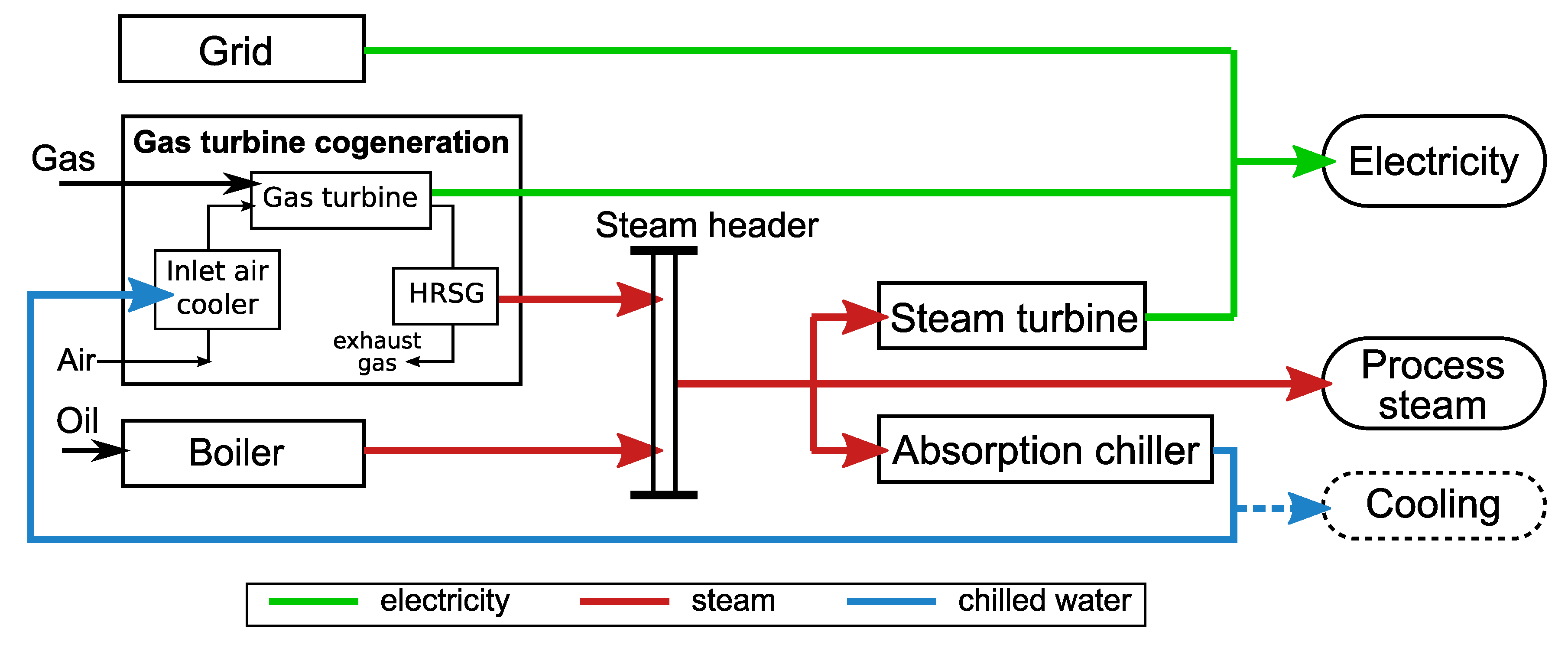
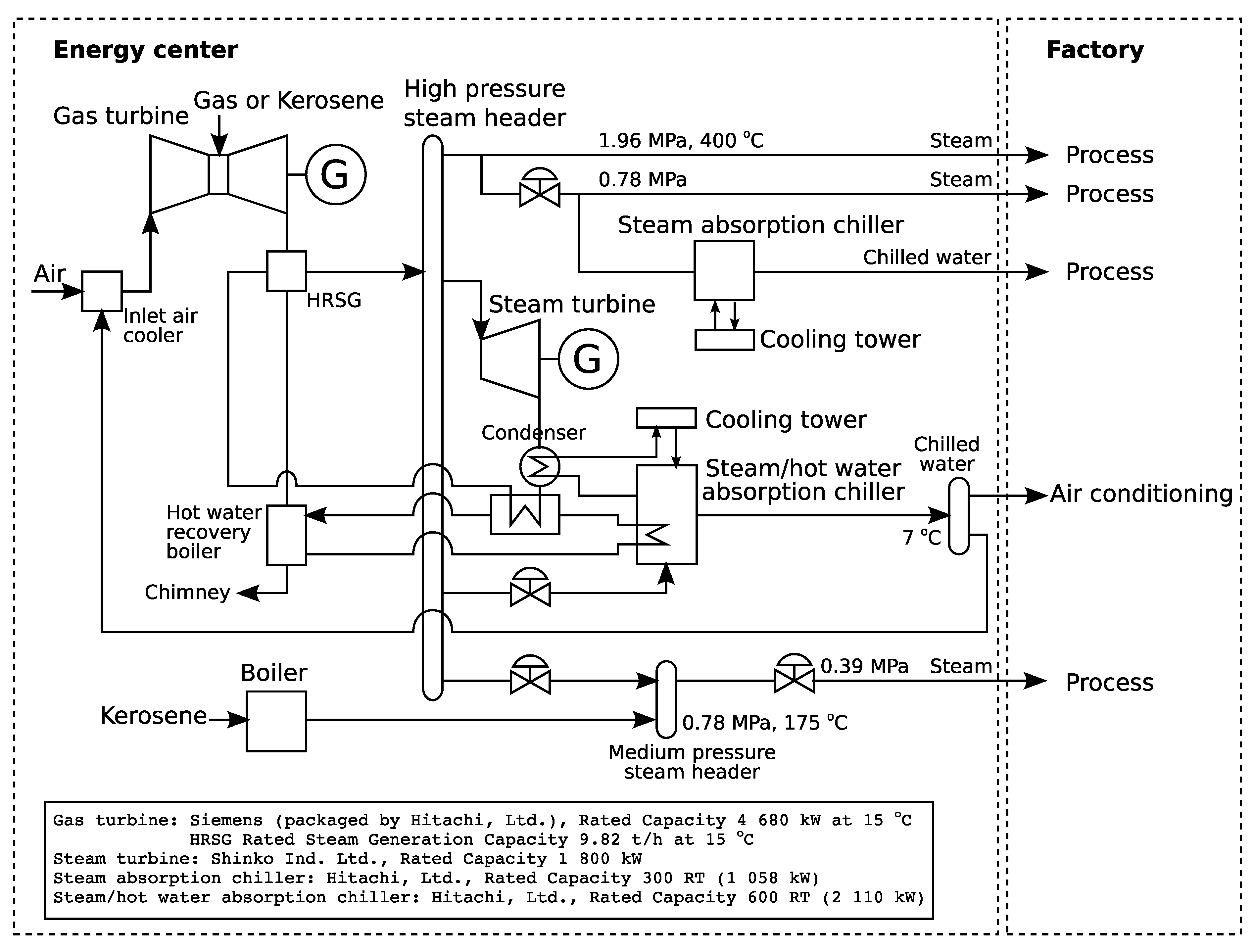
The gas turbine cogeneration system was expressed as a mathematical programming model. The system consisted of a gas turbine including an inlet air cooler and a heat recovery steam generator (HRSG), a steam turbine, an absorption chiller, a boiler and the electricity grid. Figure 1 shows the energy flow of the system. Electricity, process steam, and cooling for process or for air-conditioning are typical demands in industry, and they can be provided by multiple suppliers. In the analysis, cooling demands other than for inlet air cooling were not taken into account, and therefore, the absorption chiller would work only to provide inlet air cooling of the gas turbine. The electricity was treated as the electric power in kilowatts, and the steam and the chilled water were treated as the heat flow rates in kilowatts so that the energy balance can be expressed in the same units.

Figure 1. The energy flow of the simplified gas turbine cogeneration system with the turbine inlet air cooling.

Figure 1. The energy flow of the simplified gas turbine cogeneration system with the turbine inlet air cooling.

The supplied electric power and heat flow rate of the steam should be greater than or equal to the demands, which can be expressed by Eqs. (1-2).

$$\begin{array}{cc}\hfill x_{\mathrm{e}}& \le x_{\mathrm{G}}+x_{\mathrm{GT}}+x_{\mathrm{ST}}\hfill \end{array}$$

(1)

$$\begin{array}{cc}\hfill x_{\mathrm{s}}& \le x_{\mathrm{B}}+{\rho }_{\mathrm{GT}}{x}_{\mathrm{GT}}-{\omega }_{\mathrm{ST}}{x}_{\mathrm{ST}}-{\omega }_{\mathrm{AC}}{x}_{\mathrm{AC}}\hfill \end{array}$$

(2)

where, $x_{\mathrm{e}}$ and $x_{\mathrm{s}}$ represent the electric power demand and the heat flow rate of the steam demand. The electric power supply from the grid, the gas turbine and the steam turbine are denoted by $x_{\mathrm{G}}$, $x_{\mathrm{GT}}$ and $x_{\mathrm{ST}}$, respectively. $x_{\mathrm{B}}$ denotes the heat flow rate of steam from the boiler, and $x_{\mathrm{AC}}$ denotes the heat flow rate of chilled water from the absorption chiller. The ratio of the heat flow rate of steam from the HRSG to the electric power from the gas turbine is denominated the steam to electricity ratio, and denoted by ${\rho }_{\mathrm{GT}}$. Then, ${\rho }_{\mathrm{GT}}{x}_{\mathrm{GT}}$ represents the heat flow rate of steam from the gas turbine cogeneration. The steam consumption ratios of the steam turbine and the absorption chiller are given as ${\omega }_{\mathrm{ST}}$ and ${\omega }_{\mathrm{AC}}$, respectively. The former is equivalent to the inverse of the efficiency based on the steam input, and the latter is equivalent to the inverse of the coefficient of performance.

The inlet air cooling of the gas turbine enhances the maximum output from the gas turbine. By introducing the capacity of the gas turbine, $X_{\mathrm{GT}}$, the effect of the inlet air cooling was expressed by Eq. (3).

$$x_{\mathrm{GT}}\le X_{\mathrm{GT}}+{\alpha }_{\mathrm{GT}}{x}_{\mathrm{AC}}$$

(3)

It was assumed that the increment of the gas turbine capacity was proportional to the heat flow rate of chilled water supplied to the gas turbine. The proportional constant is denoted by ${\alpha }_{\mathrm{GT}}$.

In addition to the enhancement of the gas turbine capacity, the inlet air cooling improves the electric efficiency of the gas turbine. Provided that the improvement is proportional to the heat flow rate of chilled water to the gas turbine, the fuel consumption of the gas turbine can be expressed as ${\omega }_{\mathrm{GT}}{x}_{\mathrm{GT}}-{\beta }_{\mathrm{GT}}{x}_{\mathrm{AC}}$, where ${\omega }_{\mathrm{GT}}$ is the fuel consumption ratio without the inlet air cooling and ${\beta }_{\mathrm{GT}}$ is the improvement factor of the fuel consumption by the inlet air cooling.

As the objective of the optimization is the minimization of the energy cost during a certain time period, $\Delta t$, the energy cost should be expressed as a function of $x_{\mathrm{G}}$, $x_{\mathrm{GT}}$, $x_{\mathrm{ST}}$, $x_{\mathrm{B}}$ and $x_{\mathrm{AC}}$. By defining the unit energy prices of the electricity, gas and oil as $P_{\mathrm{e}}$, $P_{\mathrm{g}}$ and $P_{\mathrm{o}}$, respectively, the energy cost, C, can be given as:

$$C=P_{\mathrm{e}}{x}_{\mathrm{G}}\Delta t+P_{\mathrm{g}}({\omega }_{\mathrm{GT}}{x}_{\mathrm{GT}}-{\beta }_{\mathrm{GT}}{x}_{\mathrm{AC}})\Delta t+P_{\mathrm{o}}{\omega }_{\mathrm{B}}{x}_{\mathrm{B}}\Delta t$$

(4)

where, ${\omega }_{\mathrm{B}}$ is the fuel consumption ratio of the boiler, which is equivalent to the inverse of the thermal efficiency.

All the parameters that represent the characteristics of equipment, such as ${\omega }_{\mathrm{GT}}$, ${\omega }_{\mathrm{ST}}$, ${\omega }_{\mathrm{AC}}$, ${\omega }_{\mathrm{B}}$, ${\rho }_{\mathrm{GT}}$, ${\alpha }_{\mathrm{GT}}$ and ${\beta }_{\mathrm{GT}}$, were assumed to be constant so that the system could be modeled by the linear programming. Therefore, the part load characteristics of equipment were linearly approximated.

2.2. The Mathematical Formulation and the Optimal Solution

From Eqs. (1–4), the optimization problem is formed as follows:

$$\begin{array}{cc}\hfill \text{Minimize:}& f\left(\mathit{x}\right)=C\hfill \end{array}$$

(5)

$$\begin{array}{cc}\hfill \text{Subject}\text{to:}& g_1\left(\mathit{x}\right)=x_{\mathrm{e}}-x_{\mathrm{G}}-x_{\mathrm{GT}}-x_{\mathrm{ST}}\le 0\hfill \end{array}$$

(6)

$$\begin{array}{cc}& g_2\left(\mathit{x}\right)=x_{\mathrm{s}}-x_{\mathrm{B}}-{\rho }_{\mathrm{GT}}{x}_{\mathrm{GT}}+{\omega }_{\mathrm{ST}}{x}_{\mathrm{ST}}+{\omega }_{\mathrm{AC}}{x}_{\mathrm{AC}}\le 0\hfill \end{array}$$

(7)

$$\begin{array}{cc}& g_3\left(\mathit{x}\right)=x_{\mathrm{GT}}-X_{\mathrm{GT}}-{\alpha }_{\mathrm{GT}}{x}_{\mathrm{AC}}\le 0\hfill \end{array}$$

(8)

where, $\mathit{x}=(x_{\mathrm{G}},x_{\mathrm{GT}},x_{\mathrm{ST}},x_{\mathrm{B}},x_{\mathrm{AC}})$. Using the Lagrange multipliers, $\mathit{\lambda }=({\lambda }_1,{\lambda }_2,{\lambda }_3)$, the objective function can be expressed by the Lagrangian, $L(\mathit{x},\mathit{\lambda })$.

$$\begin{array}{cc}\hfill L(\mathit{x},\mathit{\lambda })& =f\left(\mathit{x}\right)+{\mathit{\lambda }}^{\mathit{T}}\mathit{g}\left(\mathit{x}\right)\hfill \\ & =C+{\lambda }_1(x_{\mathrm{e}}-x_{\mathrm{G}}-x_{\mathrm{GT}}-x_{\mathrm{ST}})+{\lambda }_2(x_{\mathrm{s}}-x_{\mathrm{B}}-{\rho }_{\mathrm{GT}}{x}_{\mathrm{GT}}+{\omega }_{\mathrm{ST}}{x}_{\mathrm{ST}}+{\omega }_{\mathrm{AC}}{x}_{\mathrm{AC}})\hfill \\ & +{\lambda }_3(x_{\mathrm{GT}}-X_{\mathrm{GT}}-{\alpha }_{\mathrm{GT}}{x}_{\mathrm{AC}})\hfill \end{array}$$

(9)

According to the Kuhn-Tucker conditions, x and λ satisfy the following conditions at the optimal solution.

$$\begin{array}{c}\frac{\partial L(\mathit{x},\mathit{\lambda })}{\partial x_i}\ge 0\end{array}$$

(10)

$$\begin{array}{c}{x}_i\frac{\partial L(\mathit{x},\mathit{\lambda })}{\partial x_i}=0\end{array}$$

(11)

$$\begin{array}{c}{\lambda }_j{g}_j\left(\mathit{x}\right)=0\end{array}$$

(12)

$$\begin{array}{c}{x}_i,{\lambda }_j\ge 0\\ i=\text{G,}\text{GT,}\text{ST,}\text{B,}\text{AC},j=1,2,3\end{array}$$

(13)

The following inequalities are derived from Eq. (10).

$$\begin{array}{cc}\hfill \mathrm{G}:& P_{\mathrm{e}}\Delta t-{\lambda }_1\ge 0\hfill \end{array}$$

(14)

$$\begin{array}{cc}\hfill \mathrm{GT}:& P_{\mathrm{g}}{\omega }_{\mathrm{GT}}\Delta t-{\lambda }_1-{\rho }_{\mathrm{GT}}{\lambda }_2+{\lambda }_3\ge 0\hfill \end{array}$$

(15)

$$\begin{array}{cc}\hfill \mathrm{ST}:& -{\lambda }_1+{\omega }_{\mathrm{ST}}{\lambda }_2\ge 0\hfill \end{array}$$

(16)

$$\begin{array}{cc}\hfill \mathrm{B}:& P_{\mathrm{o}}{\omega }_{\mathrm{B}}\Delta t-{\lambda }_2\ge 0\hfill \end{array}$$

(17)

$$\begin{array}{cc}\hfill \mathrm{AC}:& -P_{\mathrm{g}}{\beta }_{\mathrm{GT}}\Delta t+{\omega }_{\mathrm{AC}}{\lambda }_2-{\alpha }_{\mathrm{GT}}{\lambda }_3\ge 0\hfill \end{array}$$

(18)

Equation (11) means that $x_i>0$ if the derived expression concerning the supplier i satisfies the equality, otherwise, $x_i=0$. For example, $x_{\mathrm{G}}$ has a positive value if ${\lambda }_1$ equals $P_{\mathrm{e}}\Delta t$. If ${\lambda }_1$ is less than $P_{\mathrm{e}}\Delta t$, then $x_{\mathrm{G}}$ equals zero.

With regard to the constraint $g_3\left(\mathit{x}\right)$, it is possible to classify the gas turbine operation into two conditions. The first one is the case where the electric power from the gas turbine is less than the capacity, which means $x_{\mathrm{G}}<X_{\mathrm{GT}}+{\alpha }_{\mathrm{GT}}{x}_{\mathrm{AC}}$. The second one is the case where the electric power from the gas turbine is at the maximum, which means $x_{\mathrm{GT}}=X_{\mathrm{GT}}+{\alpha }_{\mathrm{GT}}{x}_{\mathrm{AC}}$. We denominate the former and the latter conditions the operational conditions I and II, respectively. Due to Eq. (12) of the Kuhn-Tucker condition, ${\lambda }_3=0$ on the operational condition I, and ${\lambda }_3>0$ on the operational condition II.

2.3. The Optimal Solution where the Electric Power from the Gas Turbine is less than the Capacity

On the operational condition I where $x_{\mathrm{G}}<X_{\mathrm{GT}}+{\alpha }_{\mathrm{GT}}{x}_{\mathrm{AC}}$, Eqs. (14–18) can be drawn on the ${\lambda }_1$-${\lambda }_2$ plane because ${\lambda }_3$ equals zero. The region surrounded by the inequalities gives the feasible solutions, and the output of the supplier i has a positive value, i.e. $x_i>0$, when the solution exists on the line which represents the supplier i.

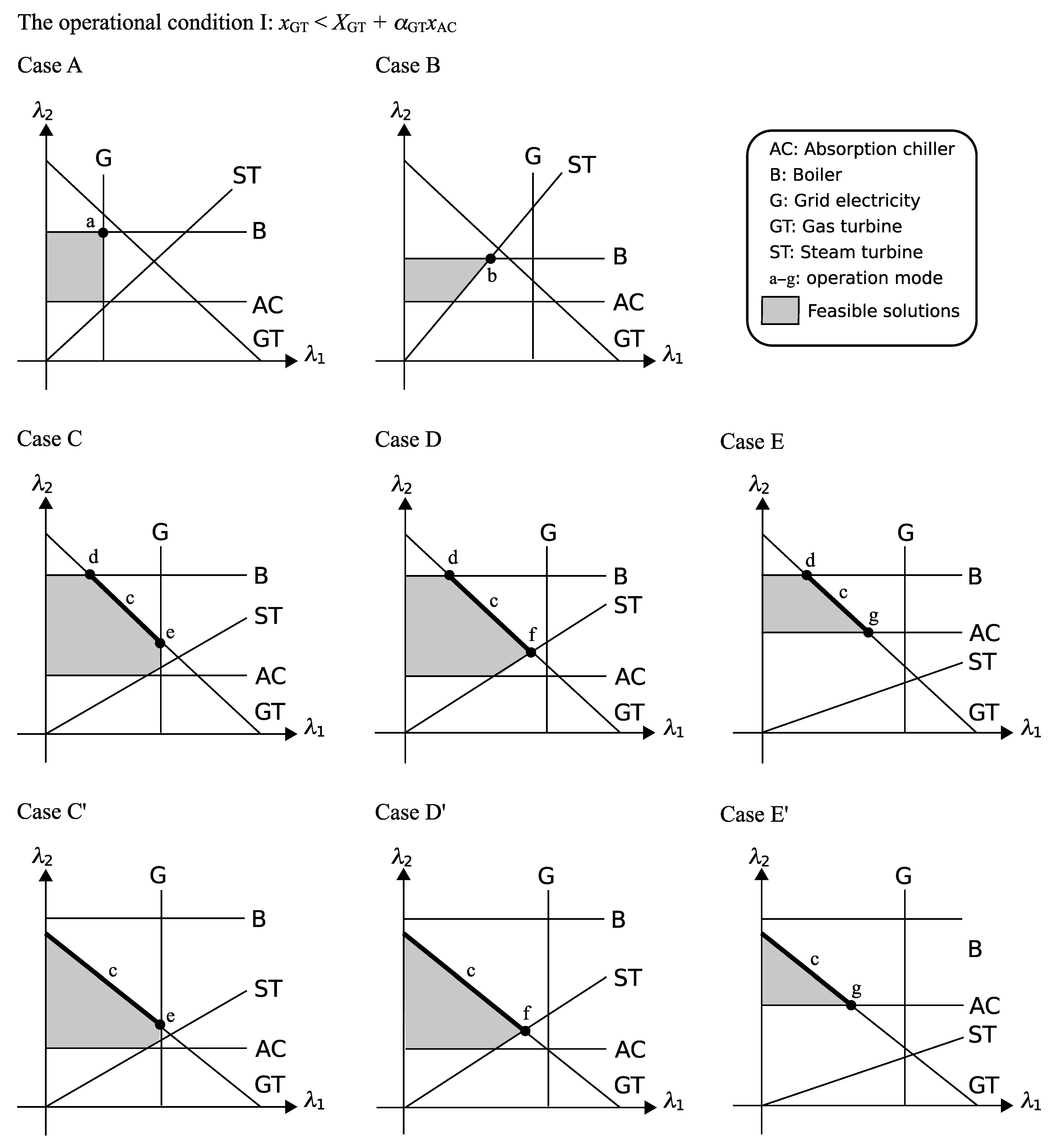
Figure 2 illustrates eight cases of the feasible solution region appeared on the ${\lambda }_1$-${\lambda }_2$ plane. The possible optimal solutions are marked as the operation modes “a" to “g". The mode a appears in the case A, where the grid electricity and the boiler are chosen at the optimal operation. In the mode b, the boiler and the steam turbine satisfy the electric power demand and the heat flow rate of the steam demand. After the case C, the electric power from the gas turbine is positive at the optimal operation. In the case C, the optimal operation is the gas turbine only (mode c), the combination of the gas turbine and the boiler (mode d) or the combination of the gas turbine and the grid electricity (mode e). In this case, the optimal operation will be chosen by the ratio of the heat flow rate of the steam demand to the electric power demand, which will be discussed later. When the line which represents the boiler does not cross the gas turbine line in the first quadrant, which is the case C’, only the modes c and e appear as the possible optimal solutions. The modes f and g appear in the cases D and E, respectively. The suppliers chosen at each mode are summarized in Table 1.

Table 1. The combination of suppliers at each mode.

Mode	Grid	Boiler	Gas Turbine	Steam Turbine	Absorption Chiller
a	⊠	⊠	□	□	□
b	□	⊠	□	⊠	□
c	□	□	⊠	□	□
d	□	⊠	⊠	□	□
e	⊠	□	⊠	□	□
f	□	□	⊠	⊠	□
g	□	□	⊠	□	⊠
h	□	⊠	⊠	□	⊠
i	⊠	□	⊠	□	⊠
j	□	□	⊠	⊠	⊠

Table 1. The combination of suppliers at each mode.

Mode	Grid	Boiler	Gas Turbine	Steam Turbine	Absorption Chiller
a	⊠	⊠	□	□	□
b	□	⊠	□	⊠	□
c	□	□	⊠	□	□
d	□	⊠	⊠	□	□
e	⊠	□	⊠	□	□
f	□	□	⊠	⊠	□
g	□	□	⊠	□	⊠
h	□	⊠	⊠	□	⊠
i	⊠	□	⊠	□	⊠
j	□	□	⊠	⊠	⊠

The cases A through E will occur depending on the performance parameters of the suppliers and the unit energy prices. The conditions of each case can be obtained from the graphical analysis. For example, the case A occurs if ${\lambda }_1$ at the intersection of G and B is smaller than that at the intersection of GT and B, and is smaller than that at the intersection of ST and B. In addition, the line B has to be located above the line AC so that the feasible solution region exists. Then, the following conditions can be derived.

$$\begin{array}{c}{P}_{\mathrm{e}}+{\rho }_{\mathrm{GT}}{\omega }_{\mathrm{B}}{P}_{\mathrm{o}}\le {\omega }_{\mathrm{GT}}{P}_{\mathrm{g}}\end{array}$$

(19)

$$\begin{array}{c}{P}_{\mathrm{e}}\le {\omega }_{\mathrm{ST}}{\omega }_{\mathrm{B}}{P}_{\mathrm{o}}\end{array}$$

(20)

$$\begin{array}{c}{\omega }_{\mathrm{B}}{\omega }_{\mathrm{AC}}{P}_{\mathrm{o}}\ge {\beta }_{\mathrm{GT}}{P}_{\mathrm{g}}\end{array}$$

(21)

Equation (19) means that the gas cost to produce a certain quantity of electricity and steam with the gas turbine is higher than the total of the electricity and oil costs to purchase the same quantity of electricity from the grid and to produce the same quantity of steam with the boiler. Equation (20) means that the electricity cost to purchase a certain quantity of electricity is cheaper than the oil cost to produce the same quantity of electricity using the boiler and the steam turbine. Equation (21) indicates that the reduction of the gas cost by a certain quantity of the inlet air cooling should be smaller than the oil cost to provide the same quantity of cooling using the boiler and the absorption chiller. Otherwise, the optimal solution does not exist because the reduction of the gas cost is unlimited by the inlet air cooling using the absorption chiller driven by the boiler.

Figure 2. The possible cases of the optimal solution on the operational condition I.

Figure 2. The possible cases of the optimal solution on the operational condition I.

Similarly, the following conditions can be derived for the other cases. The condition given as Eq. (21) has to be applied to all the cases below.

Case B:

$$\begin{array}{c}({\rho }_{\mathrm{GT}}+{\omega }_{\mathrm{ST}}){\omega }_{\mathrm{B}}{P}_{\mathrm{o}}\le {\omega }_{\mathrm{GT}}{P}_{\mathrm{g}}\end{array}$$

(22)

$$\begin{array}{c}{P}_{\mathrm{e}}\ge {\omega }_{\mathrm{ST}}{\omega }_{\mathrm{B}}{P}_{\mathrm{o}}\end{array}$$

(23)

Equation (22) compares the production cost of the electricity and the steam between the gas and the oil. The gas cost to produce a certain quantity of electricity and steam by the gas turbine is higher than the oil cost to produce the same quantity of electricity and steam by the combination of the boiler and the steam turbine. Equation (23) is the opposite of Eq. (20), which means that the oil cost to produce a certain quantity of electricity by the boiler and the steam turbine is cheaper than the purchase price of electricity.

Case C:

$$\begin{array}{c}{P}_{\mathrm{e}}+{\rho }_{\mathrm{GT}}{\omega }_{\mathrm{B}}{P}_{\mathrm{o}}\ge {\omega }_{\mathrm{GT}}{P}_{\mathrm{g}}\end{array}$$

(24)

$$\begin{array}{c}{\omega }_{\mathrm{GT}}{P}_{\mathrm{g}}\ge {\rho }_{\mathrm{GT}}{\omega }_{\mathrm{B}}{P}_{\mathrm{o}}\end{array}$$

(25)

$$\begin{array}{c}{\omega }_{\mathrm{GT}}{P}_{\mathrm{g}}\ge \left(1+\frac{{\rho }_{\mathrm{GT}}}{{\omega }_{\mathrm{ST}}}\right)P_{\mathrm{e}}\end{array}$$

(26)

$$\begin{array}{c}\left({\omega }_{\mathrm{GT}}-\frac{{\rho }_{\mathrm{GT}}{\beta }_{\mathrm{GT}}}{{\omega }_{\mathrm{AC}}}\right)P_{\mathrm{g}}\ge P_{\mathrm{e}}\end{array}$$

(27)

Equation (24) is the opposite case of Eq. (19). Equation (25) compares the boiler and the gas turbine regarding the steam production, which is related to the mode d. In the case C, the oil cost for the boiler is cheaper than the gas cost for the gas turbine to produce a certain quantity of steam. If the gas cost is cheaper, mode d is not a candidate for the optimal solution, as illustrated in the case C’. Equations (26) and (27) evaluate the effectiveness of the steam turbine and the inlet air cooling by the absorption chiller, respectively. The grid electricity is superior to the steam turbine and to the inlet air cooling in this case.

Case D:

In addition to Eq. (25),

$$\begin{array}{c}({\rho }_{\mathrm{GT}}+{\omega }_{\mathrm{ST}}){\omega }_{\mathrm{B}}{P}_{\mathrm{o}}\ge {\omega }_{\mathrm{GT}}{P}_{\mathrm{g}}\end{array}$$

(28)

$$\begin{array}{c}{\omega }_{\mathrm{GT}}{P}_{\mathrm{g}}\le \left(1+\frac{{\rho }_{\mathrm{GT}}}{{\omega }_{\mathrm{ST}}}\right)P_{\mathrm{e}}\end{array}$$

(29)

$$\begin{array}{c}\frac{{\omega }_{\mathrm{GT}}{\omega }_{\mathrm{AC}}}{{\beta }_{\mathrm{GT}}}-{\rho }_{\mathrm{GT}}\ge {\omega }_{\mathrm{ST}}\end{array}$$

(30)

Similarly to the case C’, the case D’ occurs if the inequality sign of Eq. (25) is reversed. Equation (28) is the opposite case of Eq. (22), which is the comparison of the electricity production between gas and oil. Equation (29) is the opposite case of Eq. (26), which is the comparison of the steam turbine and grid electricity. The gas cost to produce a certain quantity of electricity by the combination of the gas turbine and the steam turbine is cheaper than the purchase cost of the same quantity of electricity from the grid. Equation (30) gives the condition where the steam turbine is more advantageous than the inlet air cooling by the absorption chiller. The left hand side of Eq. (30) represents an additional steam required for a certain quantity of electricity production by the inlet air cooling. Therefore, Eq. (30) insists that the steam required for a certain quantity of electricity production by the steam turbine is smaller than that required for the same quantity of electricity production by the inlet air cooling in this case, and it is independent of energy prices.

Case E:

In addition to Eq. (25),

$$\begin{array}{c}\left({\omega }_{\mathrm{GT}}-\frac{{\rho }_{\mathrm{GT}}{\beta }_{\mathrm{GT}}}{{\omega }_{\mathrm{AC}}}\right)P_{\mathrm{g}}\le P_{\mathrm{e}}\end{array}$$

(31)

$$\begin{array}{c}\frac{{\omega }_{\mathrm{GT}}{\omega }_{\mathrm{AC}}}{{\beta }_{\mathrm{GT}}}-{\rho }_{\mathrm{GT}}\le {\omega }_{\mathrm{ST}}\end{array}$$

(32)

The case E’ occurs if Eq. (25) is reversed. Equations (31) and (32) are the opposite cases of Eqs. (27) and (30), which give the conditions where the inlet air cooling is more advantageous compared with the alternative technologies. In this case, Eq. (28) is always satisfied because of Eqs. (21) and (32).

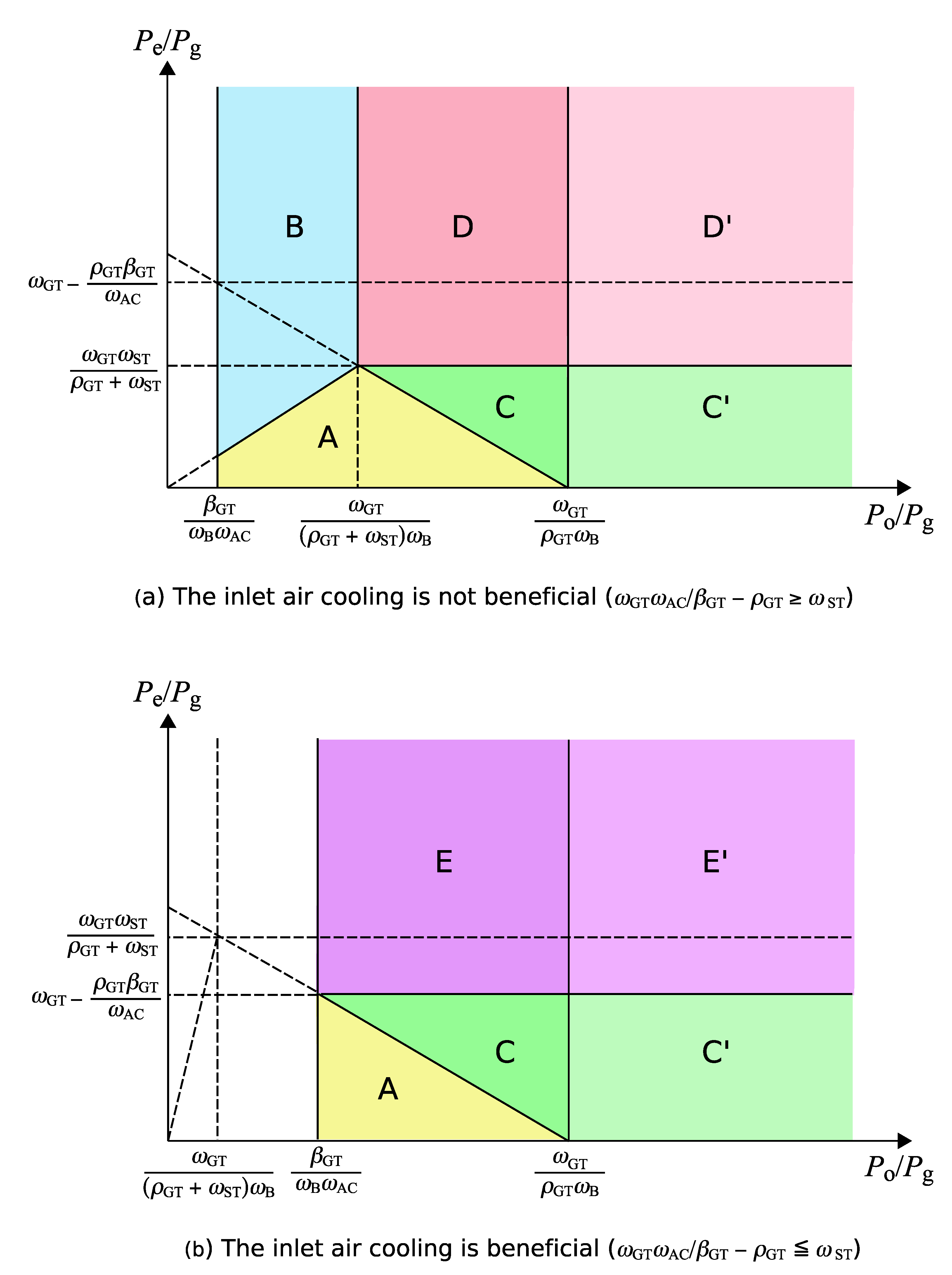
The conditions discussed above can be arranged using the relative electricity price, $P_{\mathrm{e}}/P_{\mathrm{g}}$ and the relative oil price, $P_{\mathrm{o}}/P_{\mathrm{g}}$. The optimal cases to be chosen are graphically shown in Figure 3 on the $P_{\mathrm{o}}/P_{\mathrm{g}}$-$P_{\mathrm{e}}/P_{\mathrm{g}}$ plane. When Eq. (30) is valid, Figure 3 (a) should be applied. The inlet air cooling is not an optimal option in any case. When Eq. (32) is valid, the cases E and E’ appear on the plane and the steam turbine is never chosen, as depicted in Figure 3 (b). It is noteworthy that if the inlet air cooling cannot improve the gas turbine efficiency, i.e. ${\beta }_{\mathrm{GT}}=0$, the inlet air cooling is never the optimal solution.

As the cases C, D and E include three operation modes, another criterion for the selection of the optimal operation mode is necessary in those cases. The additional criterion is related with the steam to electricity ratio, and can be derived from the consideration below.

In the cases C, D and E, ${\lambda }_1$ and ${\lambda }_2$ have positive values. Therefore, two of the constraints given as Eqs. (6) and (7) take the equality conditions due to the Kuhn-Tucker condition Eq. (12). Then, the two equations can be solved simultaneously for two variables which have positive values at each mode.

For the mode d, the simultaneous equations can be solved under $x_{\mathrm{GT}}\text{,}{x}_{\mathrm{B}}>0$ and $x_{\mathrm{G}}\text{,}{x}_{\mathrm{ST}}\text{,}{x}_{\mathrm{AC}}=0$. Then, one can obtain $x_{\mathrm{GT}}=x_{\mathrm{e}}$ and $x_{\mathrm{B}}=x_{\mathrm{s}}-{\rho }_{\mathrm{GT}}{x}_{\mathrm{e}}$. Because $x_{\mathrm{B}}$ has a positive value, the following condition has to be satisfied for the mode d to be selected.

$${\rho }_{\mathrm{GT}}<\frac{x_{\mathrm{s}}}{x_{\mathrm{e}}}$$

(33)

At the mode e, one can obtain $x_{\mathrm{G}}=x_{\mathrm{e}}-x_{\mathrm{s}}/{\rho }_{\mathrm{GT}}$ and $x_{\mathrm{GT}}=x_{\mathrm{s}}/{\rho }_{\mathrm{GT}}$, and the following condition can be drawn out of the former expression because $x_{\mathrm{G}}$ is greater than zero at this mode.

$${\rho }_{\mathrm{GT}}>\frac{x_{\mathrm{s}}}{x_{\mathrm{e}}}$$

(34)

Similar considerations can be applied to the cases D and E. Consequently, Eq. (33) is the condition for the mode d to be selected, while Eq. (34) is the condition for the modes e, f or g to be selected. Furthermore, it is obvious that the mode c has to be chosen if the steam to electricity ratio of the gas turbine is equal to the ratio of the heat flow rate of the steam demand to the electric power demand, i.e. ${\rho }_{\mathrm{GT}}=x_{\mathrm{s}}/x_{\mathrm{e}}$.

Equations (33) and (34) mean that when the steam to electricity ratio of the gas turbine is smaller than the ratio of the heat flow rate of the steam demand to the electric power demand, the gas turbine should be operated to meet the electric power demand. Then, the boiler should balance the heat flow rate of the steam supply with the demand. On the other hand, if the steam to electricity ratio of the gas turbine is larger than the ratio of the heat flow rate of the steam demand to the electric power demand, the gas turbine has to be operated to meet the heat flow rate of the steam demand. Then, the insufficient electric power supply from the gas turbine has to be compensated by either the grid (mode e), the steam turbine (mode f), or the inlet air cooling (mode g). There is no need of any auxiliary equipment to supply additional electric power or steam if the steam to electricity ratio of the gas turbine matches the demands.

Figure 3. The optimal operation cases expressed on the relative oil price-relative electricity price plane (the operational condition I).

Figure 3. The optimal operation cases expressed on the relative oil price-relative electricity price plane (the operational condition I).

2.4. The Optimal Solution where the Electric Power from the Gas Turbine is at the Maximum

In the operational condition II, the third constraint, Eq. (8), takes the equality condition and ${\lambda }_3$ would have a positive value. Then, Eqs. (15) and (18) yields:

$$({\rho }_{\mathrm{GT}}-\frac{{\omega }_{\mathrm{AC}}}{{\alpha }_{\mathrm{GT}}}){\lambda }_2\le -{\lambda }_1+P_{\mathrm{g}}({\omega }_{\mathrm{GT}}-\frac{{\beta }_{\mathrm{GT}}}{{\alpha }_{\mathrm{GT}}})\Delta t$$

(35)

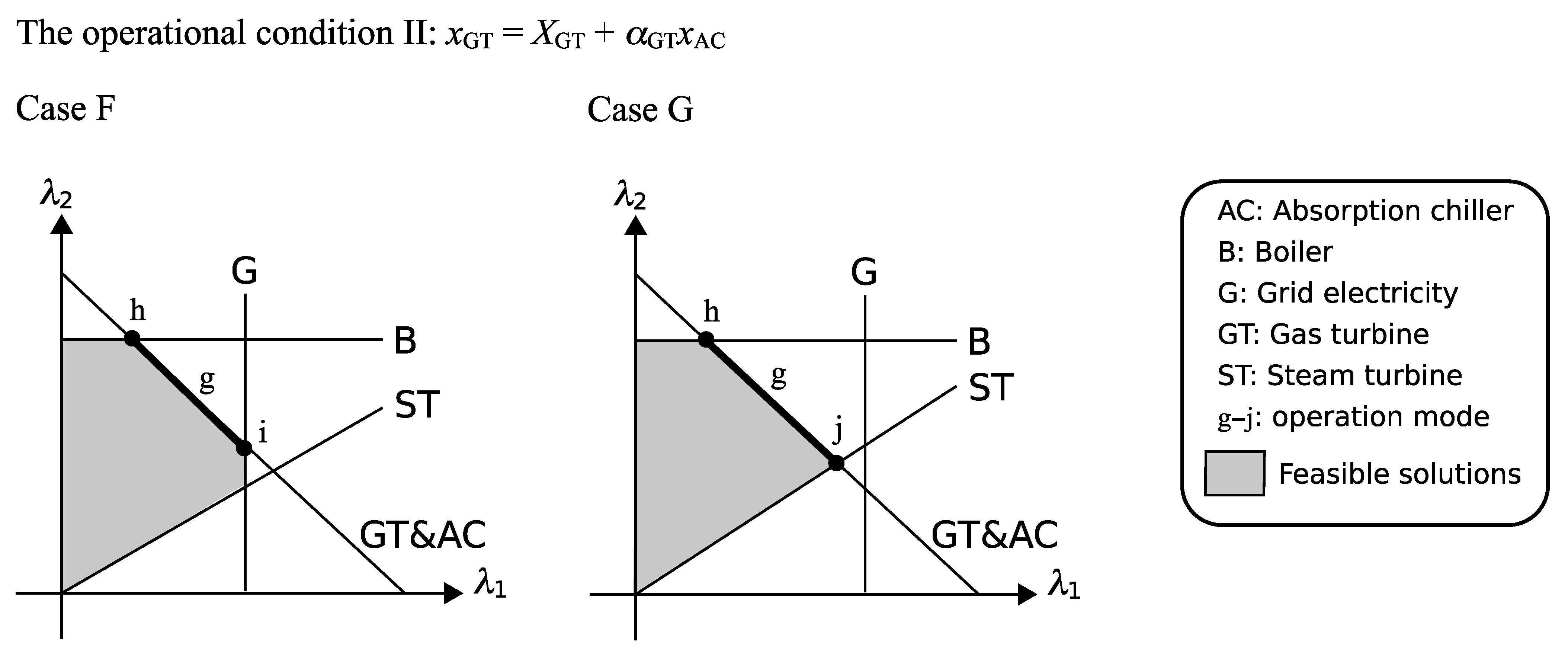
It is reasonable to assume that ${\rho }_{\mathrm{GT}}-\frac{{\omega }_{\mathrm{AC}}}{{\alpha }_{\mathrm{GT}}}>0$ and ${\omega }_{\mathrm{GT}}-\frac{{\beta }_{\mathrm{GT}}}{{\alpha }_{\mathrm{GT}}}>0$ in the case of gas turbine cogeneration systems because of relatively low electric efficiency (≈ 25 %) and a high heat to electricity ratio (${\rho }_{\mathrm{GT}}>1.4$). Then, the optimal solution cases can be defined by a similar consideration to the operational condition I, and the newly appeared cases are illustrated in Figure 4. The cases F and G can occur in the operational condition II in addition to the cases A and B of the operational condition I. Similarly to the cases C’ and D’ of the operational condition I, the cases F’ and G’ can be defined where the mode h is excluded from the cases F and G, respectively.

Figure 4. The optimal solution cases on the operational condition II.

Figure 4. The optimal solution cases on the operational condition II.

In the operational condition II, the conditions of the cases A and B are slightly different from those in the operational condition I, as given below.

Case A:

$$\begin{array}{c}{P}_{\mathrm{e}}+{\omega }_{\mathrm{B}}\left({\rho }_{\mathrm{GT}}-\frac{{\omega }_{\mathrm{AC}}}{{\alpha }_{\mathrm{GT}}}\right)P_{\mathrm{o}}\le \left({\omega }_{\mathrm{GT}}-\frac{{\beta }_{\mathrm{GT}}}{{\alpha }_{\mathrm{GT}}}\right)P_{\mathrm{g}}\end{array}$$

(36)

$$\begin{array}{c}{P}_{\mathrm{e}}\le {\omega }_{\mathrm{ST}}{\omega }_{\mathrm{B}}{P}_{\mathrm{o}}\end{array}$$

(37)

Case B:

$$\begin{array}{c}{\omega }_{\mathrm{B}}\left({\omega }_{\mathrm{ST}}+{\rho }_{\mathrm{GT}}-\frac{{\omega }_{\mathrm{AC}}}{{\alpha }_{\mathrm{GT}}}\right)P_{\mathrm{o}}\le \left({\omega }_{\mathrm{GT}}-\frac{{\beta }_{\mathrm{GT}}}{{\alpha }_{\mathrm{GT}}}\right)P_{\mathrm{g}}\end{array}$$

(38)

$$\begin{array}{c}{P}_{\mathrm{e}}\ge {\omega }_{\mathrm{ST}}{\omega }_{\mathrm{B}}{P}_{\mathrm{o}}\end{array}$$

(39)

The conditions for the cases F and G are obtained as follows.

Case F:

$$\begin{array}{c}{P}_{\mathrm{e}}+{\omega }_{\mathrm{B}}\left({\rho }_{\mathrm{GT}}-\frac{{\omega }_{\mathrm{AC}}}{{\alpha }_{\mathrm{GT}}}\right)P_{\mathrm{o}}\ge \left({\omega }_{\mathrm{GT}}-\frac{{\beta }_{\mathrm{GT}}}{{\alpha }_{\mathrm{GT}}}\right)P_{\mathrm{g}}\end{array}$$

(40)

$$\begin{array}{c}\left({\omega }_{\mathrm{GT}}-\frac{{\beta }_{\mathrm{GT}}}{{\alpha }_{\mathrm{GT}}}\right)P_{\mathrm{g}}\ge {\omega }_{\mathrm{B}}\left({\rho }_{\mathrm{GT}}-\frac{{\omega }_{\mathrm{AC}}}{{\alpha }_{\mathrm{GT}}}\right)P_{\mathrm{o}}\end{array}$$

(41)

$$\begin{array}{c}\left({\omega }_{\mathrm{GT}}-\frac{{\beta }_{\mathrm{GT}}}{{\alpha }_{\mathrm{GT}}}\right)P_{\mathrm{g}}\ge \left[1+\frac{1}{{\omega }_{\mathrm{ST}}}\left({\rho }_{\mathrm{GT}}-\frac{{\omega }_{\mathrm{AC}}}{{\alpha }_{\mathrm{GT}}}\right)\right]P_{\mathrm{e}}\end{array}$$

(42)

Case G:

In addition to Eq. (41),

$$\begin{array}{c}{\omega }_{\mathrm{B}}\left({\omega }_{\mathrm{ST}}+{\rho }_{\mathrm{GT}}-\frac{{\omega }_{\mathrm{AC}}}{{\alpha }_{\mathrm{GT}}}\right)P_{\mathrm{o}}\ge \left({\omega }_{\mathrm{GT}}-\frac{{\beta }_{\mathrm{GT}}}{{\alpha }_{\mathrm{GT}}}\right)P_{\mathrm{g}}\end{array}$$

(43)

$$\begin{array}{c}\left({\omega }_{\mathrm{GT}}-\frac{{\beta }_{\mathrm{GT}}}{{\alpha }_{\mathrm{GT}}}\right)P_{\mathrm{g}}\le \left[1+\frac{1}{{\omega }_{\mathrm{ST}}}\left({\rho }_{\mathrm{GT}}-\frac{{\omega }_{\mathrm{AC}}}{{\alpha }_{\mathrm{GT}}}\right)\right]P_{\mathrm{e}}\end{array}$$

(44)

The cases F’ and G’ occur when the inequality sign of Eq. (41) is reversed. Equations (36), (38), (40), (41), (42), (43) and (44) correspond to Eqs. (19), (22), (24), (25), (26), (28) and (29), respectively. In these equations, ${\omega }_{\mathrm{GT}}-\frac{{\beta }_{\mathrm{GT}}}{{\alpha }_{\mathrm{GT}}}$ is substituted for ${\omega }_{\mathrm{GT}}$, and ${\rho }_{\mathrm{GT}}-\frac{{\omega }_{\mathrm{AC}}}{{\alpha }_{\mathrm{GT}}}$ is substituted for ${\rho }_{\mathrm{GT}}$.

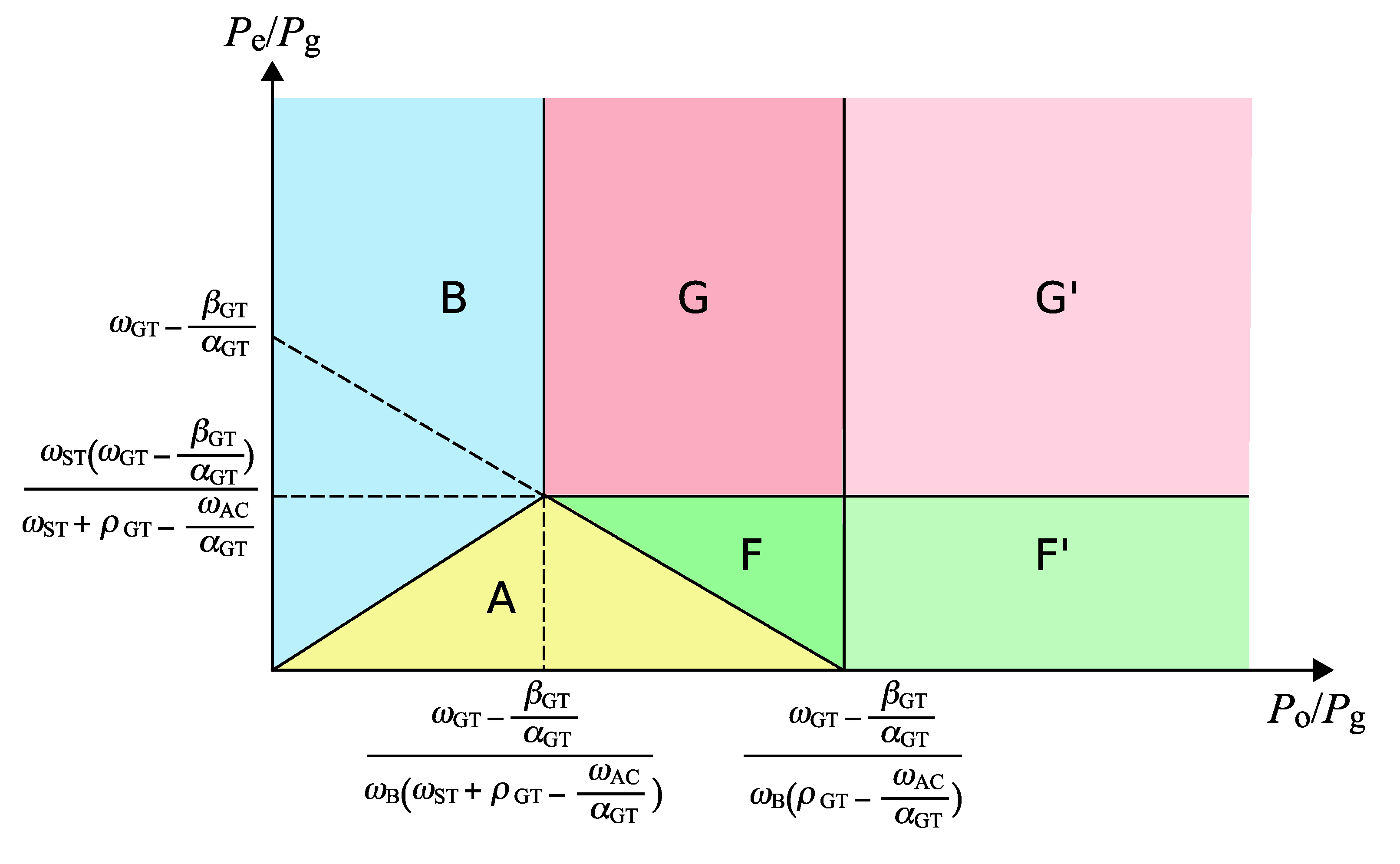
The optimal cases of the operational condition II are illustrated on the $P_{\mathrm{o}}/P_{\mathrm{g}}$-$P_{\mathrm{e}}/P_{\mathrm{g}}$ plane as shown in Figure 5. Unlike the operational condition I, there is no lower limit of the relative oil price for the optimal solution to exist. The line separating the cases F and G is determined by the multiple parameters. Basically, a larger ${\rho }_{\mathrm{GT}}$ or a smaller ${\omega }_{\mathrm{ST}}$ lowers the line, which causes a higher possibility for the case G to be selected.

Figure 5. The optimal operation cases expressed on the relative oil price-relative electricity price plane (the operational condition II).

Figure 5. The optimal operation cases expressed on the relative oil price-relative electricity price plane (the operational condition II).

To find the optimal mode out of three operation modes included in the cases F or G, another strategy is necessary. The additional conditions can be found by a similar examination on the variables to that done for the cases C, D and E. In the operational condition II, three variables can be analytically solved by the constraints given as Eqs. (6), (7) and (8) taking equality conditions.

In the mode g, only two variables, $x_{\mathrm{GT}}$ and $x_{\mathrm{AC}}$, are positive and the other variables are equal to zero. Therefore, the analytical solutions of those in the operational condition II can be obtained from equations derived from Eqs. (6) and (7) as $x_{\mathrm{GT}}=x_{\mathrm{e}}$ and $x_{\mathrm{AC}}=({\rho }_{\mathrm{GT}}{x}_{\mathrm{e}}-x_{\mathrm{s}})/{\omega }_{\mathrm{AC}}$. Then the third constraint gives the equality condition concerning $x_{\mathrm{s}}/x_{\mathrm{e}}$ and $X_{\mathrm{GT}}/x_{\mathrm{e}}$ as follows:

$$\frac{x_{\mathrm{s}}}{x_{\mathrm{e}}}={\rho }_{\mathrm{GT}}-\frac{{\omega }_{\mathrm{AC}}}{{\alpha }_{\mathrm{GT}}}\left(1-\frac{X_{\mathrm{GT}}}{x_{\mathrm{e}}}\right)$$

(45)

where, $X_{\mathrm{GT}}/x_{\mathrm{e}}$ represents the ratio of the gas turbine capacity to the electricity demand, and $X_{\mathrm{GT}}/x_{\mathrm{e}}\le 1$.

For mode h, the condition where this mode should be selected is derived from the analytical solution of $x_{\mathrm{B}}$ with $x_{\mathrm{B}}>0$ as follows:

$$\frac{x_{\mathrm{s}}}{x_{\mathrm{e}}}>{\rho }_{\mathrm{GT}}-\frac{{\omega }_{\mathrm{AC}}}{{\alpha }_{\mathrm{GT}}}\left(1-\frac{X_{\mathrm{GT}}}{x_{\mathrm{e}}}\right)$$

(46)

For the mode i, $x_{\mathrm{G}}>0$ and $x_{\mathrm{AC}}>0$ give the following two conditions.

$$\begin{array}{c}\frac{x_{\mathrm{s}}}{x_{\mathrm{e}}}<{\rho }_{\mathrm{GT}}-\frac{{\omega }_{\mathrm{AC}}}{{\alpha }_{\mathrm{GT}}}\left(1-\frac{X_{\mathrm{GT}}}{x_{\mathrm{e}}}\right)\end{array}$$

(47)

$$\begin{array}{c}\frac{x_{\mathrm{s}}}{x_{\mathrm{e}}}>{\rho }_{\mathrm{GT}}\frac{X_{\mathrm{GT}}}{x_{\mathrm{e}}}\end{array}$$

(48)

For the mode j, $x_{\mathrm{ST}}>0$ and $x_{\mathrm{AC}}>0$ give the following conditions.

$$\begin{array}{c}\frac{x_{\mathrm{s}}}{x_{\mathrm{e}}}<{\rho }_{\mathrm{GT}}-\frac{{\omega }_{\mathrm{AC}}}{{\alpha }_{\mathrm{GT}}}\left(1-\frac{X_{\mathrm{GT}}}{x_{\mathrm{e}}}\right)\end{array}$$

(49)

$$\begin{array}{c}\frac{x_{\mathrm{s}}}{x_{\mathrm{e}}}>({\omega }_{\mathrm{ST}}+{\rho }_{\mathrm{GT}})\frac{X_{\mathrm{GT}}}{x_{\mathrm{e}}}-{\omega }_{\mathrm{ST}}\end{array}$$

(50)

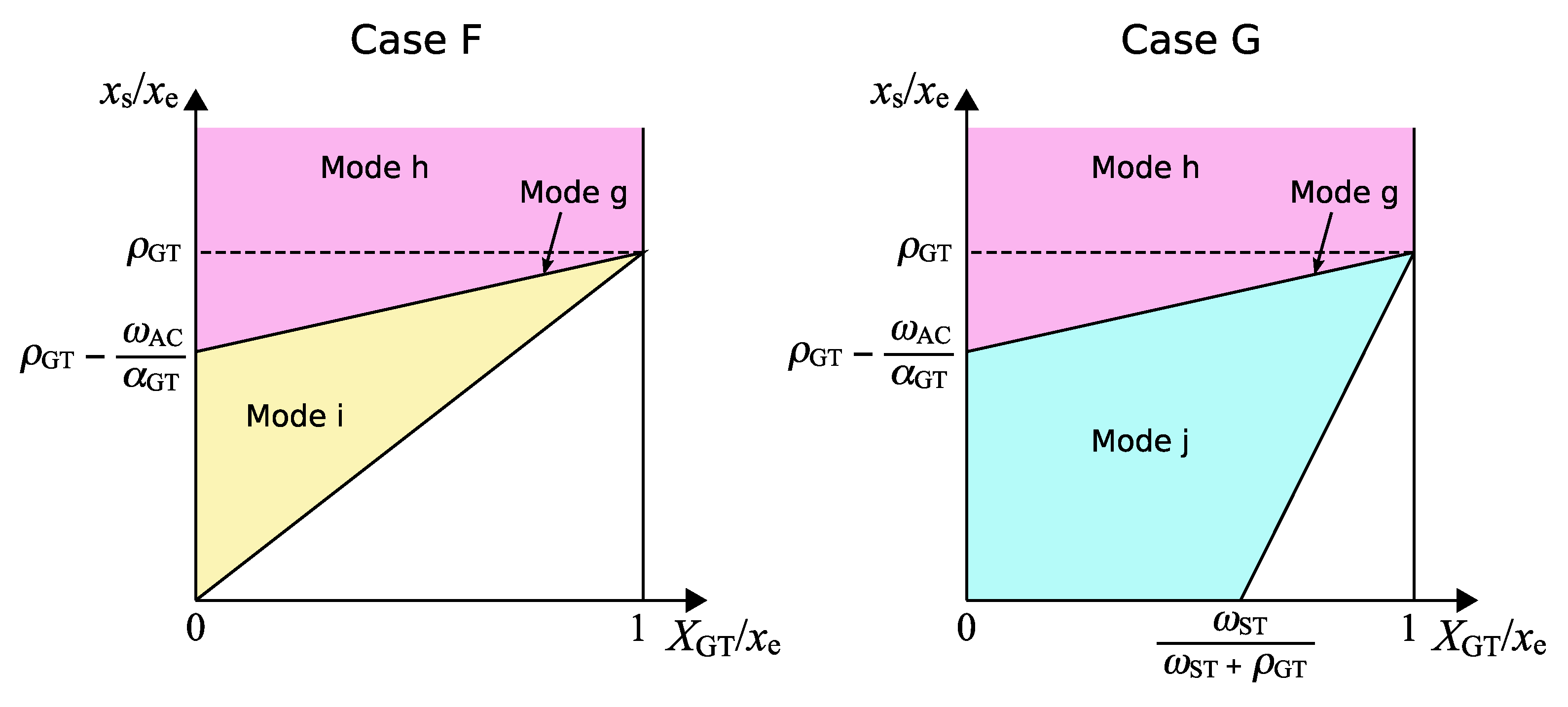
The conditions given as Eqs. (45–50) are graphically shown in Figure 6. In the cases F and G, the operational condition II cannot be applied to the region of $\frac{x_{\mathrm{s}}}{x_{\mathrm{e}}}<{\rho }_{\mathrm{GT}}\frac{X_{\mathrm{GT}}}{x_{\mathrm{e}}}$ and $\frac{x_{\mathrm{s}}}{x_{\mathrm{e}}}<({\omega }_{\mathrm{ST}}+{\rho }_{\mathrm{GT}})\frac{X_{\mathrm{GT}}}{x_{\mathrm{e}}}-{\omega }_{\mathrm{ST}}$, respectively, because $x_{\mathrm{AC}}$ becomes negative in this region. The optimal operation should be found under the operational condition I in this region.

3. Comparison of the Optimal Operation Criteria with a Detailed Optimization Result

To examine the applicability of the method explained in the previous section to a practical cogeneration system, the combination of the suppliers selected by the optimal operation criteria was compared with the results of a detailed optimization of an existing plant.

3.1. An Example of an Existing Energy Center of a Factory

An energy center of an existing factory is depicted in Figure 7. The factory is located in Aichi Prefecture, Japan, and produces car-related parts. The energy center produces electricity by a combined cycle of a gas turbine and a steam turbine. The gas turbine can be fueled with either gas or kerosene, and it is equipped with an inlet air cooler. The electric power distribution system of the factory is also linked to the electricity grid so that the electricity can be purchased in case the electric power supply from the energy center is insufficient.

The steam is produced from the gas turbine and boilers. The high, medium or low pressure steam is consumed in the manufacturing process as well as for the driving force of the steam turbine and absorption chillers. The absorption chillers supply chilled water for the process, air conditioning and the inlet air cooling. One of the absorption chiller can utilize hot water recovered from the low temperature waste gas of the gas turbine to enhance the heat recovery efficiency of the system.

Figure 6. The selection of the optimal operation mode in the cases of F and G.

Figure 6. The selection of the optimal operation mode in the cases of F and G.

Figure 7. An energy center of a factory.

Figure 7. An energy center of a factory.

3.2. The Performance Characteristics of the Equipment

The part load characteristics of the equipment were linearly approximated so that the system could be modeled by the linear programming. The approximation lines were derived from the characteristics of the existing machines used in the energy center.

The electricity and the steam generation characteristics of the gas turbine and the HRSG are shown in Figure 8, for example. The electric capacity of the gas turbine increases with lower inlet air temperatures. The quantity of generated steam is also augmented with lower inlet air temperatures.

In practice, it is known that the inlet air cooling is beneficial when the purchase of the grid electricity will exceed the power contract without the augmentation of the gas turbine capacity. Furthermore, the inlet air cooling is effective when the outdoor air temperature is higher than 15 °C. A part of the operation of the actual gas turbine system is based on the above judgement of the operator, which is also included in the detailed optimization model.

Figure 8. The performance characteristics of the gas turbine and the HRSG.

Figure 8. The performance characteristics of the gas turbine and the HRSG.

3.3. The Detailed Optimization of the Energy Center

The optimization of the system shown in Figure 7 was performed by a software tool developed for this system. The optimization method used in the tool is the linear programming method combined with the listed start-stop patterns of equipment and with the judgement whether the inlet air cooling is on or off. The methodology used in the tool is fully described in the reference [11].

The Detailed Optimization Method

The energy flow in the energy center was modeled by the linear programming. The outputs of equipment were the variables to be optimized, whose values could be varied within the lower and upper limits. To make the optimization model realistic, it is necessary to take the start-stop patterns of the equipment into account. The start-stop patterns were generated according to the possible operation conditions of the actual energy center, and 20 patterns were chosen for the enumeration. The optimal solution was searched by the combination of the enumeration of the start-stop patterns and the linear programming method. The list of the start-stop patterns of the gas turbine and the steam turbine is given in Figure 9.

The demands given in the detailed optimization are shown in Figure 10 as the ratios of the heat flow rate of the steam demand to the electric power demand on a summer day with a large electric power demand and on a winter day with a small steam demand. On the summer day, the ratio of the heat flow rate of the steam demand to the electric power demand is at a low level throughout a day. While, it is high on the winter day, and during the hours 2 to 6, the ratio exceeds 1.4 that is the steam to electricity ratio of the gas turbine.

Figure 9. The start-stop patterns of the gas turbine and the steam turbine.

Figure 9. The start-stop patterns of the gas turbine and the steam turbine.

The Plant Operation Obtained by the Detailed Optimization

The accumulated graphs shown in Figure 11 through Figure 14 illustrate the electric power supply and the heat flow rate of the steam supply from equipment on the summer and winter days. On the summer day, the gas turbine and the steam turbine worked at the maximum load and the electric power demand was met by the purchase from the grid for most of the day except the hours 2 to 6, at which the electric power demand was small. The inlet air cooling of the gas turbine was used only at the hours 10 and 14, at which the peak of the electric power demand existed. The steam was mainly supplied by the gas turbine, and the boiler was used only if the total heat flow rate of the steam demands by the process, the steam turbine, and the absorption chiller exceeded the maximum heat flow rate of the steam from the gas turbine.

Figure 10. The ratio of the heat flow rate of the steam demand to the electric power demand on a summer day and on a winter day.

Figure 10. The ratio of the heat flow rate of the steam demand to the electric power demand on a summer day and on a winter day.

On the winter day, the steam turbine was less used compared with the usage on the summer day because of the smaller electric power demand. The grid electricity was used only if the electric power demand exceeded the total capacity of the gas turbine and the steam turbine, as shown at the hours 10 and 14. Because the gas turbine was operated to follow the electric power demand, the boiler operated when the heat flow rate of the steam from the gas turbine was not sufficient.

3.4. The Comparison of the Optimal Operation Criteria with the Detailed Optimization Results

The optimal operation criteria were applied to the existing energy center, and the optimal operation suggested by the optimal operation criteria was compared with the detailed optimization results given in Figure 11, Figure 12, Figure 13 and Figure 14. The optimal operation criteria and the detailed optimization method are different in that the former indicates the combination of equipment to be operated, while the latter gives the quantities of electric power and the heat flow rate of the steam from the equipment.

Figure 11. The hourly variation of the electric power supply and demand on a summer day.

Figure 11. The hourly variation of the electric power supply and demand on a summer day.

Figure 12. The hourly variation of the heat flow rate of steam supply and demand on a summer day.

Figure 12. The hourly variation of the heat flow rate of steam supply and demand on a summer day.

Figure 13. The hourly variation of the electric power supply and demand on a winter day.

Figure 13. The hourly variation of the electric power supply and demand on a winter day.

Figure 14. The hourly variation of the heat flow rate of steam supply and demand on a winter day.

Figure 14. The hourly variation of the heat flow rate of steam supply and demand on a winter day.

The performance of equipment was assumed as given in Table 2. The values of the parameters, ${\alpha }_{\mathrm{GT}}$, ${\beta }_{\mathrm{GT}}$ and ω, used to find the optimal operation criteria are also given in Table 2. The prices of electricity, gas and kerosene were given as 9 yen/kW h, 3 yen/kW h and 4 yen/kW h, respectively.

Table 2. Equipment performance

Gas turbine electric efficiency	25 %	(${\omega }_{\mathrm{GT}}$ = 4.0)
Gas turbine steam to electricity ratio	1.4
Steam turbine efficiency (steam input basis)	30 %	(${\omega }_{\mathrm{ST}}$ = 3.3)
Absorption chiller COP	1.2	(${\omega }_{\mathrm{AC}}$ = 0.83)
Boiler thermal efficiency	85 %	(${\omega }_{\mathrm{B}}$ = 1.2)
Gas turbine alpha number	${\alpha }_{\mathrm{GT}}$ = 1.1
Gas turbine beta number	${\beta }_{\mathrm{GT}}$ = 0.3

Table 2. Equipment performance

Gas turbine electric efficiency	25 %	(${\omega }_{\mathrm{GT}}$ = 4.0)
Gas turbine steam to electricity ratio	1.4
Steam turbine efficiency (steam input basis)	30 %	(${\omega }_{\mathrm{ST}}$ = 3.3)
Absorption chiller COP	1.2	(${\omega }_{\mathrm{AC}}$ = 0.83)
Boiler thermal efficiency	85 %	(${\omega }_{\mathrm{B}}$ = 1.2)
Gas turbine alpha number	${\alpha }_{\mathrm{GT}}$ = 1.1
Gas turbine beta number	${\beta }_{\mathrm{GT}}$ = 0.3

The Optimal Operation Mode Selection by the Optimal Operation Criteria

By evaluating Eq. (30) or (32) using the values given in Table 2, it was found that the map shown in Figure 3 (a) should be applied to this plant under operational condition I. In addition, Figure 5 is valid under the operational condition II because ${\rho }_{\mathrm{GT}}-\frac{{\omega }_{\mathrm{AC}}}{{\alpha }_{\mathrm{GT}}}>0$ and ${\omega }_{\mathrm{GT}}-\frac{{\beta }_{\mathrm{GT}}}{{\alpha }_{\mathrm{GT}}}>0$. Then, we can substitute the values in Table 2 for the parameters in Figure 3 (a) and Figure 5, and examine the relative prices of the system, which are $P_{\mathrm{e}}/P_{\mathrm{g}}=3.0$ and $P_{\mathrm{o}}/P_{\mathrm{g}}=1.3$.

The cases A, C and D exist within the area of $0.71\le P_{\mathrm{o}}/P_{\mathrm{g}}\le 2.4$, and the cases C and D are separated at $P_{\mathrm{e}}/P_{\mathrm{g}}=2.8$ in the case of the operational condition I. Therefore, the system falls on the area of the case D. The case D includes the modes c, d and f, and the appropriate mode can be found according to the ratio of the heat flow rate of the steam demand to the electric power demand. Under the operational condition II, the cases A, F and G exist within the area of $0.79\le P_{\mathrm{o}}/P_{\mathrm{g}}\le 4.8$ and the line dividing the cases F and G exists at $P_{\mathrm{e}}/P_{\mathrm{g}}=3.1$. Then, the case F would be selected. The optimal mode could be found by examining the ratio of the gas turbine capacity to the electric power demand and the ratio of the heat flow rate of the steam demand to the electric power demand using Figure 6. The relative electricity price is, however, in the vicinity of the interface between the cases for both of the operational conditions. Therefore, the results implied that the electric power supplies from the grid and from the steam turbine were almost equivalent in terms of electricity production cost for this plant.

Assuming that the electric power demand and the heat flow rate of the steam demand during a day are predictable, the operational condition of the energy center can be forecasted by comparing the electric power demand with the maximum capacity of the gas turbine. In the case of the energy center, the electric power demand is the total of the electric power output of the suppliers illustrated in Figure 11 and Figure 13 because the demand and the supply should be balanced. The maximum capacity of the gas turbine is about 5 100 kW as shown in Figure 8 (a). Therefore, it is known that the optimal operation should be found under the operational condition I during the hours 2–6 and under the operational condition II during the rest of the hours on the summer day. On the other hand, the system is under the operational condition II only at the hours 10 and 14, and is under the operational condition I for the rest of the hours on the winter day.

Then, the operation mode at each hour can be chosen according to the ratio of the heat flow rate of the steam demand to the electric power demand given in Figure 10 under the operational condition of the hour. The operation mode and the suppliers to be operated at each hour are summarized in Figure 15.

Figure 15. The operation mode suggested by the optimal operation criteria at each hour on the summer and the winter days.

Figure 15. The operation mode suggested by the optimal operation criteria at each hour on the summer and the winter days.

The Applicability of the Optimal Operation Criteria to the Energy Center

During the hours 2–6 on the winter day, the optimal operation criteria suggested the mode d. The operation chosen by the detailed optimization method for the period agreed with the mode d where the gas turbine supplied both the electric power and the steam and the boiler complementarily supplied the steam. Similarly, the detailed optimization results agreed with the optimal operation criteria during the hours 2–6 on the summer day, where the electric power was supplied by the combination of the gas turbine and the steam turbine and the steam was supplied by the heat recovery from the gas turbine (mode f). In these cases, the system obviously operated under the operation condition I because the electric power demand was far below the gas turbine capacity. The optimal operation criteria could provide the optimal combination of the suppliers when the electric power and the heat flow rate of the steam from the suppliers were free from the restrictions by the capacities.

Besides the hours 2–6, the system was under the operational condition I at the hours 1, 7–24 on the winter day except the hours 10 and 14. The optimal operation criteria suggested the mode f. Although the mode f was essentially in agreement with the detailed optimization results, a discrepancy was observed for the steam supply. If the system followed the optimal operation criteria, the heat recovery from the gas turbine should be sufficient to meet the heat flow rate of the steam demand. The boiler, however, supplied the steam in addition to the heat recovery from the gas turbine in the detailed optimization results. The main reason of the discrepancy would be that the operation of the steam turbine was restricted by the start-stop patterns given in Figure 9. Even if the electric power demand decreased around the peak hours, the steam turbine could not be shut down because of the fixed start-stop pattern. Therefore, the electric power from the gas turbine had to be reduced, which resulted in the insufficiency of the heat recovery from the gas turbine and the auxiliary steam supply from the boiler.

The system was under the operational condition II during the hours 1, 7–24 on the summer day and at the hours 10 and 14 on the winter day. The optimal operation criteria suggested the mode i for these hours, where the suppliers were the gas turbine, the inlet air cooling with the absorption chiller and the grid electricity for the electric power, and the heat recovery from the gas turbine for the steam. The inlet air cooling was, however, used only at the hours 10 and 14 on the summer day in the detailed optimization results because the operation of the inlet air cooling depended on whether the grid electricity would exceed the power contract as well as on whether the outdoor air temperature was higher than 15 ${}^{\circ }$C. These judgement were not included in the optimal operation criteria.

In addition to that, the electric power demand was much larger than the total capacity of the gas turbine and the steam turbine. Therefore, both the steam turbine and the grid electricity were used for the electric power supply in addition to the gas turbine in the detailed optimization results. This situation is different from the mode i because the power contract of the grid electricity and the capacity of the steam turbine are unlimited in the optimal operation criteria.

In a real system, it is usual that the capacities of the suppliers have to be taken into account to find the optimal operation. The optimal operation criteria are applicable to that situation by the following mannar. If the total capacity of the suppliers chosen by the optimal operation criteria is smaller than the demand, it is obvious that the suppliers chosen have to be operated at the full load. Then, the second best suppliers can be found by judgement based on the conditions given in Eqs. (19)–(32). For example, given that the gas turbine and the steam turbine are at the full load and an additional electric power supplier is required, the tertiary electric power supplier can be found by evaluating Eq. (27) or (31), which compares the grid electricity and the inlet air cooling. If Eq. (27) is valid, the grid electricity is the choice.

4. Conclusions

The study demonstrated the optimal operation criteria of a gas turbine cogeneration system based on the analytical solution of a linear programming model. The optimal operation criteria give the combination of equipment to provide electricity and steam with the minimum energy cost using the energy prices and the performance of equipment. It was shown that the optimal operation of the system could be represented by the relative prices of electricity and oil against the price of gas, as well as the ratio of the heat flow rate of the steam demand to the electric power demand.

To confirm the applicability, the optimal operation criteria were compared with the results of a detailed optimization method for an existing cogeneration plant. The results showed a good agreement between the optimal operation criteria and the detailed optimization results under the condition where the electric power and the heat flow rate of the steam from the suppliers were free from the restrictions imposed by the capacities. The discrepancy between the optimal operation criteria and the detailed optimization method would arise if the operation of the supplier was dominated by the fixed start-stop pattern and by the capacity of the supplier. It is usual that the operation of multiple suppliers are restricted by their capacities. Under that situation, the optimal operation criteria can suggest the second best suppliers by evaluating the conditions that provide the comparison between the alternative suppliers.

The advantage of the optimal operation criteria is that it facilitates the operation of the system to achieve the minimum energy cost. Cogeneration plant operators can choose the optimal combination of machines to be operated based on a map that shows the operation cases. Even if the plant is automatically operated by the energy management system, the optimal operation criteria would help the operators to check the optimal operation and to detect any abnormality.

References and Notes

1. Yokoyama, R.; Ito, K.; Matsumoto, Y. Optimal sizing of a gas turbine cogeneration plant in consideration of its operational strategy. J. Eng. Gas Turbines Power 1994, 116, 32–38. [Google Scholar] [CrossRef]
2. Beihong, Z.; Weiding, L. An optimal sizing method for cogeneration plants. Energ. Bldg. 2006, 38, 189–195. [Google Scholar] [CrossRef]
3. Kong, X.Q.; Wang, R.Z.; Huang, X.H. Energy optimization model for a CCHP system with available gas turbines. Appl. Therm. Eng. 2005, 25, 377–391. [Google Scholar] [CrossRef]
4. Manolas, D.A.; Frangopoulos, C.A.; Gialamas, T.P.; Tsahalis, D.T. Operation optimization of an industrial cogeneration system by a genetic algorithm. Energ. Conv. Manage. 1997, 38, 1625–1636. [Google Scholar] [CrossRef]
5. Brooks, F.J. GE Gas Turbine Performance Characteristics. In GE Reference Documents; GER-3567H; pp. 1–16.
6. U.S. Environmental Protection Agency, Combined Heat and Power Partnership. Technology Characterization: Gas Turbines. In Catalog of CHP Technologies; 2008. [Google Scholar]
7. Ondryas, I.S.; Wilson, D.A.; Kawamoto, M.; Haub, G.L. Options in gas turbine power augmentation using inlet air chilling. J. Eng. Gas Turbines Power 1991, 113, 203–211. [Google Scholar] [CrossRef]
8. Alhazmy, M.M.; Najjar, Y.S.H. Augmentation of gas turbine performance using air coolers. Appl. Therm. Eng. 2004, 24, 415–429. [Google Scholar] [CrossRef]
9. Chacartegui, R.; Jimenez-Espadafor, F.; Sanchez, D.; Sanchez, T. Analysis of combustion turbine inlet air cooling systems applied to an operating cogeneration power plant. Energ. Conve. Manage. 2008, 49, 2130–2141. [Google Scholar] [CrossRef]
10. Sundaram, R.K. A First Course in Optimization Theory; Cambridge University Press: New York, U.S., 1996; pp. 145–150. [Google Scholar]
11. Bannai, M.; Kashiwagi, T.; Akisawa, A.; Tsukamoto, K.; Sugiyama, S.; Harada, Y. Development of object-model-based energy management system for optimal operation of heat and co-generation facilities. Transactions of the Society of Heating, Air-Conditioning and Sanitary Engineers of Japan 2004, No.93, 57–66. (in Japanese). [Google Scholar]