North American Natural Gas Supply Forecast: The Hubbert Method Including the Effects of Institutions

Abstract

In this article, the U.S. and southern Canadian natural gas supply market is considered. An important model for oil and natural gas supply is the Hubbert curve. Not all regions of the world are producing oil or natural gas following a Hubbert curve, even when price and market conditions are accounted for. One reason is that institutions are affecting supply. We investigate the possible effects of oil and gas market institutions in North America on natural gas supply. A multi-cycle Hubbert curve with inflection points similar to the Soviet Union’s oil production multi-cycle Hubbert curve is used to determine North American natural gas discovery rates and to analyze how market specific institutions caused the inflection points. In addition, we analyze the latest shale natural gas projections critically. While currently, unconventional resources of natural gas suggest that North American natural gas production will increase without bound, the model here suggests a peak in North American natural gas supplies could happen in 2013.

1. Introduction

M. King Hubbert hypothesized an alternative method to geological estimation for determining U.S. oil supplies. His critical method of forecasting the supply of oil, particularly the peak of supply for a given region, is the Hubbert curve model [1,2,3,4], originally explained by Hubbert in 1956, but elucidated in 1962. There is a strong literature supporting it [5,6,7,8,9,10,11,12,13], including a neo-classical economic theory for why it works [14,15,16]. The curve employs a simple logistics function that Pierre François Verhulst, a Belgian mathematician, explained in 1838. Note also the word “logistic” is rooted in the Greek word for “calculating”.

Many critics have shown that the Hubbert curve does not work [17,18,19,20,21,22,23]. Not all regions of the world are producing oil or natural gas following a Hubbert curve, which suggests that either the Hubbert curve model is incorrect or it was an ad hoc model that just happened to be correct for the continental United States. The resolution of Hubbert’s accurate forecast in the U.S. with the criticisms that his method does not always work in a number of other countries can be found in the role institutions play in inhibiting exploration and production (E and P; a glossary of abbreviations and acronyms is presented before the list of references.) Thus, an important variable missing from the general Hubbert curve model may be the effect of institutions as explained in the institutional economics literature below. Since Hubbert specifically showed the possibility of a multi-cycle Hubbert curve and since the Soviet Union in particular shows such a phenomenon, this then suggests that if institutions, such as laws and rules, change drastically and affect normal market mechanisms, then those institutional changes could affect E and P patterns and require a revision of the normal Hubbert curve model using a multi-cycle Hubbert curve approach.

The key to most Hubbert forecasting is to track discovery. The U.S. Lower 48 oil discovery was close to its peak when Hubbert first predicted the oil production peak. This is why he was so accurate. Once one determines the peak in discovery, the peak in production can then be forecast. Thus a Hubbert analysis needs three things to forecast supply accurately: a significant amount of good yearly proven reserves data (i.e. yearly proven reserve estimates from a mature region from which discovery can be discerned), yearly production data, and a version of the Verhulst curve called the Richards Function [24]. Hubbert used exactly such data to create a U.S. Lower 48 logistics oil discovery trend, a logistics oil production trend, and a change in reserves trend all of which could then be statistically analyzed to forecast both the Ultimately Recoverable Resource (URR) and most importantly of all peak oil.

The problem is that one must be close to or at the peak in discovery to determine the production peak. Hubbert critics are quick to point out that a region needs to be in a mature E and P stage and needs accurate discovery data before that region’s Hubbert curve peak can be predicted; nevertheless, Hubbert accurately predicted the U.S. peak 13 years before it happened. Indubitably, a 13 year warning is better than nothing.

In this paper, we re-create Hubbert’s 1962 treatise, only instead of oil, we consider natural gas, and instead of explaining a forecast for the U.S. Lower 48, we look at the U.S. Lower 48 and southern Canada. Alaska, Northern Canada, and Mexico are either too remote to provide cost competitive supplies of natural gas to the general market in a timely manner, or as in the case of Mexico, they have national ownership institutions, which make for difficult investment decisions, which in turn affect supply. Smaller regions within the U.S. are subject to tax and regulatory changes that over time will average out but that are very difficult to analyze accurately, therefore, only a large North American region is considered. Since the data for natural gas discovery and proven reserves, even when taking price changes into account, shows huge fluctuations when compared to the data for oil in the US, this suggests that institutions have played a larger role in the natural gas discovery trend than they did in the oil trend. Therefore, instead of looking at a single natural gas discovery Hubbert curve trend with the effect of market prices, we examine a multi-cycle natural gas discovery Hubbert curve [12,25], and include a test to find where indicator variables occur in order to determine multi-cycle curve inflection points. The paper looks at institutional changes in the natural gas market to explain why the estimated indicator variable points occur when they do. We test the residuals of the model for unit roots to see if the model explains the data. We find no unit root on the residuals which suggests our model is robust.

We find clear institutional changes for the North American natural gas discovery that occur close to inflection points for a multi-cycle Hubbert curve. In addition, major changes in price expectations have affected supplies of potential gas, but normal price changes have had little effect. Furthermore, as Hubbert suggested, technology has had a slow, deliberate effect on the pattern of discovery and is actually encompassed within the Hubbert curve.

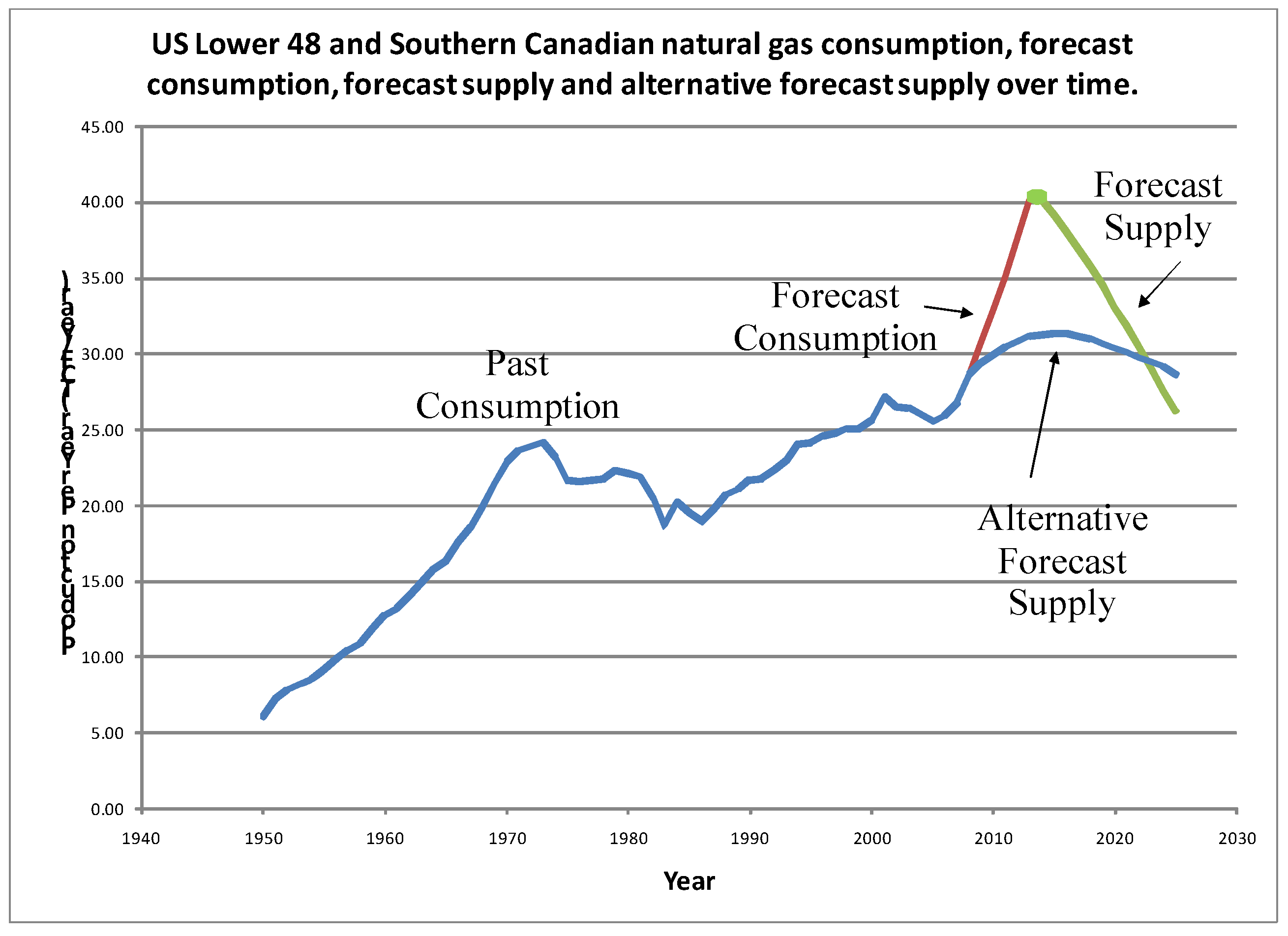
Based on the estimated discovery pattern, and considering that the discovery pattern for North American natural gas is particularly mature, a forecast of URR of natural gas is made. The Hubbert discovery pattern allows us to predict an upper bound for production based on the initial rate of production growth and the estimated URR. Based on the model, a peak in natural gas production may occur in 2013.

If production is given as a function of cumulative production rather than time, then staying below the upper bound delineated by the estimated production Hubbert curve only means we are prolonging the time, but not necessarily the cumulative production, until the peak. However if production stays below the upper bound of the Hubbert production curve past the 2013 estimate of peak production, then the peak in actual production will occur at a later date and at a higher level of cumulative production than the 2013 estimated cumulative production. However, the peak, with slightly different demand patterns, would then occur at a lower production level than the 2013 estimated peak production, possibly in 2015 as shown below.

The article is laid out as follows. In the next four sections, we consider the role of geology, of institutions, of technology and of markets respectively. Then we explain the Hubbert multi-cycle model. In Section 7 the unit root is addressed after which data and model results are given. In Section 9, price effects of the Hubbert supply model are considered, and in the next section each indicator variable is analyzed. In Section 11 a forecast for peak North American natural gas is shown, and then implications are discussed. Finally in Section 13 concluding remarks are given.

2. The Role of Geology

Before Hubbert, there were many estimates of URR of U.S. oil, suggesting a wide difference of opinion about what would happen with American oil supplies. Today we see similar speculations in regard to natural gas. For example estimates of future supplies of natural gas, based on shale rock plays, vary widely [26,27] – from as high as 5,000 trillion cubic feet (TCF) to as low as 200 TCF – which suggests that we are now searching for an answer to what will be URR of U.S. natural gas. Therefore, an alternative to the mere use of geology is needed. Reexamining Hubbert’s work can give an alternative to geological estimates of natural gas supplies as well as the URR for natural gas and an estimate for North American peak natural gas.

The typical geological method of estimating the ultimately recoverable resource is to look at crustal abundance or geologic characteristics and apply those characteristics across a wide region. The Hubbert curve by contrast uses Georgescu-Roegen’s [28] concept of “bonanza” where the tip of an iceberg is spotted. As the iceberg is examined, it proves to be a huge block—a bonanza—which creates the illusion that the ice will extend downward indefinitely and thus that increasing rates of discovery and of production of the resource in the early years of extraction—decreasing scarcity—will last forever. However, eventually scarcity is revealed when the bottom of the iceberg is ascertained.

Norgaard’s “Mayflower” problem [9] builds on this Bonanza concept where pioneers entering a frontier region are searching for farmland. The “information” and “depletion” effects [29,30,31] explain the costs of exploration and create a complete neoclassical model of resource exploration and scarcity that explains why the Hubbert curve works. A computer simulation of the search process [5] shows how a Hubbert curve works.

The Hubbert curve, while it is mostly used for oil production, can just as easily be applied to whaling in the 1800s, [6] individual coal mines, [1] individual U.S. oil states, [12] and the Hubbert curve works in experimental economic field tests, [30] because the theory behind the Hubbert curve has little to do with petroleum geology or geophysics, but rather the process of exploration [9,14,16]. The problem is to find examples of non-renewable resource extraction where institutions allow for the full and unencumbered exploitation of the resource. Whale oil/blubber, a de facto non-renewable resource due to over hunting, as well as the U.S. Lower 48 oil E and P are two of the few instances in history where there were no institutional restrictions on exploitation: the whaling example because it was a supra-national resource and the U.S. Lower 48 example because property rights were well adjudicated and there was no substantial cost problem or inhibiting regulation or state ownership of the oil mineral rights that restrained E and P. Yield per effort analyses [3,4,32] can also be used to understand natural gas supply, but for reasons of downstream bottlenecks in natural gas markets, we look only at discovery and production along the lines of Hubbert’s original 1962 treatise, and add some institutional effects [10,25].

3. The Role of Institutions

In new institutional economics literature, the effect of institutions on a developing or a transitional economy’s GDP growth rate is widely acknowledged [33]. Seminal works [34,35] show why institutions affect economic growth, where often economy wide institutions are the main instigators of economic performance. However, three levels of institutions are suggested [36], including market specific institutions—laws and regulations—that can affect specific, individual supply markets.

Oil and gas supplies around the world are under a wide variety of institutional frameworks from well adjudicated free market institutions, to production sharing arrangement (PSA) institutions, to command and control (nationalization) systems. What we would like to know is if institutions affect the supply of energy. While the investigation is limited to North American institutions and supplies, nevertheless, characteristics that occur there can help our understanding of other regions.

The conventional wisdom of institutional economics [37] is that historical accidents, such as the arrival of a particular colonial regime, can result in the placement of specific institutions on countries, and that these institutions eventually result in higher or lower growth potential. Alternatively, institutions may be endogenous [38] so that institutions are a product of economic conditions as much as a cause. As a country develops economically, its institutions change in reaction to that development. Another hypothesis is that an institutional change can be viewed in the same way as a technological change [39]. A new institutional framework that is invented or borrowed will be used if it results in an overall gain to society, otherwise it will be discarded. The bigger the gain, the more it is embraced and the more it permeates an economy.

One criticism of Hubbert’s U.S. oil supply forecast is the fact that the United States essentially had a double cycle Hubbert curve for oil starting in 1977 [40], suggesting that the change in oil prices after 1973 was a major reason for new supplies in the U.S. However, upon close examination, this second Hubbert cycle in America was due to new oil from one single state, Alaska, and the new oil came from one single region in Alaska, the North Slope. Moreover, initially the new oil on the North Slope came from one single oil field, Prudhoe Bay [41], though Prudhoe Bay was discovered in 1967, fully six years before the oil price shock of 1973. The steel pipe used for the great Trans-Alaskan pipeline to bring the oil to market was purchased in 1969, again, before the price increase. The pipeline would have been completed in 1971 had environmental laws not delayed construction. Therefore, the laws and institutions surrounding the development of North Slope oil, not prices, were the cause for the timing of the second U.S. Hubbert cycle. Indeed, had the territory of Alaska not become a state and had the State of Alaska not taken over North Slope mineral rights, making leasing rules a state, not a federal responsibility, then North Slope oil might not have been discovered until the 1970s and the battle for the pipeline would not have been resolved until the 1980s. Therefore, the role of laws and institutions is a key factor in understanding the supply of oil and natural gas.

Still if one were to hypothesize one change in Alaskan institutions that could have created the second U.S. Hubbert oil cycle, the change in status of the region from a territory to a state could not have been it, because the State of Alaska had no intention of taking the North Slope region into state hands but instead wanted to leave that region under federal jurisdiction, i.e. under the existing institutional rules, because Alaska did not have the means to regulate it. The State of Alaska changed its policy after the great earthquake of 1964, which created a need for state revenue to rebuild much of the state, and thus Alaska hoped to expedite oil exploration within the state with oil lease rules that would induce greater E and P. So the true cause of the second Hubbert cycle in the U.S. was an earthquake, not price changes and not statehood institutional changes, which shows how complicated oil and gas supply forecasting can be.

Another interesting example of institutional change is the former Soviet Union’s oil production market. The former Soviet Union changed from a Communist state to one embracing free markets after the Soviet collapse. Normally such a change would have been considered an important determinant of oil supplies. However, the former Soviet Union’s second Hubbert cycle of oil production did not happen right after the initial fall of communism, but rather it happened after the government finally sold off major oil and gas enterprises in 1996 [42], suggesting that market specific institutions surrounding mineral rights, as opposed to economy-wide institutions such as communism or democracy, are a key for determining the supply of a non-renewable resource.

This brings up cause and effect. An important technique in the study of institutions is to determine institutional changes ex ante and then statistically determine the effect of those institutional changes on economic performance [43]. The problem with this ex ante approach, as the examples of the Soviet Union and the U.S. Alaskan oil show so clearly, is that one must study in detail subtle institutional changes to reach any kind of conclusion as to their effect. The ex ante cause is never clear. As far as U.S. natural gas supply is concerned, since oil and gas are found together, then the institutional changes that we would expect to cause a change in the supply of natural gas might include important oil regulations. In addition, natural gas pipeline regulations such as the rules for permitting and for determining tariffs for pipelines can affect supply. Natural gas supply is not simply the exploration and development of the commodity, but also encompasses the transportation and marketing of the commodity as well, which means that the effect of a single law changing the upstream sector, where product is extracted, can be negated by other existing laws and regulations that bottleneck the downstream sector, where the product is transported, processed and sold. This is why the 1978 U.S. law deregulating natural gas had a large effect on supply ten years later.

However, it was not always clear to regulators that institutions were important. Before 1980, the Federal Power Commission (FPC) undoubtedly assumed that natural gas supplies could efficiently expand forever under tight regulations, and it was only after regulations were changed, i.e. de-regulation occurred, that we found out how much more supply could be had. Thus the problem with an ex ante approach especially regarding a commodity as complex as natural gas is that a simple change in one law may not have any effect. This is why even at this time it is not clear if further natural gas institutional changes can increase supplies.

An alternative idea for accounting for institutional effects is to statistically determine when a change in economic performance occurs and then look for the institutional cause. Theoretically, it should be possible to go both ways, i.e. to statistically find an effect and then search for an ex ante cause or to search for an ex ante cause first and then find an effect. However, if institutions are like technology [39], then just as technological innovations do not penetrate a market all at one time, neither will market specific institutions necessarily penetrate a market at the initiating moment of the institutional change. The effect of institutional changes can be slowed by administrations, by unrelated laws and even by court cases that determine precedence for laws. More often than not, institutional changes cannot affect a market until agencies have a chance to administer the change. Therefore, it is not necessarily the case that a specific institutional change has an immediate effect because the relationship between institutional causes and economic effects is subject to confounds.

Therefore, instead of looking at institutions themselves to determine where Hubbert curve inflection points occur, the data itself is used. The discovered inflection points can be compared to actual natural gas market events [44,45] to determine what may have been the institutional cause behind them. Once the trend in natural gas discoveries is found, a test for the effect of prices on the trend is also conducted.

4. The Role of Technology

One of the most widely mentioned criticisms of Hubbert is the effect of technology. Critics of Hubbert type scarcity analyses have suggested new technology can expand supplies above a normal Hubbert curve in many regions [46,47,48,49]. As Ryan [23] wrote:

The method Hubbert employs in projecting ultimate domestic crude oil discoveries (and production) is purely a statistical exercise and is not the result of geological or engineering analysis. … One looks in vain in Hubbert’s paper for an analysis of causes which would be sufficient to determine the ultimate level of cumulative discoveries. … Economic and technological factors which determine how much oil ultimately can be produced have changed dramatically with time and undoubtedly will continue to so do in the future.

Indeed Hubbert [1] himself has said that the bell shaped curve is not based on theory or the principles of petroleum geology, although Reynolds [14] shows that indeed there is such a theory. Nevertheless, URR does depend on technological and economic factors and can change, and as URR changes, so too would a Hubbert curve. Indeed, empirical evidence for particular regions shows that either the Hubbert curve did not work or that the Hubbert curve projections turned out to be too conservative [17].

Interestingly the term URR, has two interpretations. For example Lynch [18], among others, suggests the URR is an estimate based on current technology:

(URR refers to) the proportion of the total (resources) which is recoverable. It is logical that this should increase over time as technological advances raise the proportion of a field which can be recovered economically and as other changes lower costs and thus make it economical to produce … less productive wells.

By contrast, Hubbert himself explains that URR is based on today’s rate of change in technology, rather than on today’s level of technology [1]:

We thus do not have to worry about how much oil may be contained in known oil fields (with the Hubbert curve) over and above the American Petroleum Institute’s estimates of proved reserves, or how much improvement may be effected in the future in both exploration and productivity techniques, for those will all be added in the future as they have been in the past (emphasis added) by revision and extension in addition to new discoveries. And there is as yet no evidence of an impending departure in the future from the orderly progress which has characterized the evolution of the petroleum industry during the last hundred years.

The forecast URR within a Hubbert curve is embedded in the data itself. Accelerations (or decelerations) of technological change can indeed change the estimated final URR up (or down). In reality, technology changes smoothly [32], so the Hubbert model tracks that rate of change and incorporates all future technological changes into a forecast URR. The Hubbert URR should not be understood simply as a specific quantity that is dependent on today’s technology; rather the Hubbert URR should be understood as the forecast final reserve, based on future expected technological change. Note, many oil and gas supply models actually have a technology variable, such as a time variable, embedded in the model. The assumption is that over time, technology is improving. These technology effect variables though may be unknowingly modeling the information and depletion effects, as explained above [28,29,30], where the technology variable is actually capturing the information effect. That means that modelers are assuming technology is more powerful than it really is.

Since technology changes slowly within a normal Hubbert curve creating a smooth trend, then if sharp changes exist in a supply trend, it is indicative of non-technological changes such as changes in institutions or a very sharp change in future price expectations. For example, it is suggested that new technology is causing the sudden increase in shale natural gas supplies lately [26]. However on close inspection, there are two main technologies used to extract shale natural gas: horizontal drilling and hydro-fracturing, both of which have been used since the 1980s and the 1950s respectively. This suggests, as Hubbert emphasized, that technology has an “orderly progress” rather than a sudden impact, and therefore it is new price expectations or institutional changes that are responsible for the current shale natural gas expansion, not sudden new technology.

5. The Role of Markets

Usually, the supply of oil and gas depends on price, where high prices induce greater E and P and low prices induce less E and P, all other factors remaining the same. We also test for price effects below. However, contrary to normal economic patterns, when non-renewable natural resource extraction follows a Hubbert curve, like oil, the supply is inelastic with respect to the price for quantities above the Hubbert curve trend [11]. Therefore as long as the price of oil is above a reasonably investment-attractive level, supplies do not increase substantially above the Hubbert curve no matter how high the price or how much effort is induced. Substitutes for conventional oil, such as oil sands, coal-to-liquids and even shoes for walking, may increase with higher prices, but that is a separate issue in regards to the supply of conventional oil and natural gas. After all, if a Hubbert critic suggests an alternative to oil is available, then that is not a criticism of Hubbert analysis, it is a criticism of scarcity analysis, in which case non-Hubbert scarcity analyses should be attacked. In that case, issues such as energy return on investment (EROI), the entropy subsidy and energy grades need to be addressed [11,15,28].

However, while E and P is certainly important in regards to the supply of natural gas, there is another issue. Normally, supply in an industry depends on how many factories or producing units exist, but only marginally on transportation and logistics issues since those factories and production units can be planned around cheap transportation or near markets. Natural gas is different. Expanding natural gas supply depends not only on a natural gas well, but also critically on having a pipeline to that well. A factory can be built near a road or near a rail line but a natural gas well can only be built where the reserves are located. Therefore, the natural gas transportation system must come to the well, not the other way around as in most industries. However, unlike an oil transportation system, a natural gas transportation system requires a substantial portion of the final price of the commodity to pay for the transportation, where often natural gas pipeline tariffs are more than 50% of the final wholesale price. Oil transportation costs for example are often lower than 10% of the final wholesale price. Transportation and logistics are therefore a significant factor in natural gas supply, more so than any other industry.

This brings up the strategic problem of finding gas: should you look for natural gas before a pipeline is built, or should you build a pipeline before natural gas is discovered? The additional risk of simultaneously needing two parts to a single commodity supply solution—the natural gas well and the natural gas pipeline—makes the decision to expand natural gas supply a high risk proposition indeed, more so than a normal decision to expand supply in other industries including that of the oil industry. This means it is inappropriate to use normal Hubbert economic analyses that take into account the information effect, the depletion effect, price, extraction costs and technology change when looking at natural gas supply [13]. For example, the price and cost of oil can be an important variable in determining oil supply [10] independent of the cost to transport, but it is not so for natural gas. Furthermore, cost and technological change can be two important determinants of natural gas supply but cannot be the only determinants due to the problem of transportation.

On top of the chicken and egg dilemma for natural gas of either drilling first or building a pipeline first, there is also the problem of natural gas supplies being a natural monopoly. To gain market advantage, monopolists can easily target natural gas pipelines for acquisition in order to lower the cost of transportation, but also to constrain supply. Therefore, natural gas pipelines are by necessity highly regulated. However, regulatory approval of new natural gas pipelines can take years to sort out. So even if the expected value of a natural gas discovery is substantially greater than the expected cost of finding that natural gas, including the expected probability of the discovery, the present value of a single exploration effort can be negative due to regulatory delay since it takes so many years to permit and build a natural gas pipeline to the well before any value can be derived. The negative net present value causes explorers to refrain from searching for natural gas as a stand-alone commodity. Rather, natural gas is much more likely to be discovered when looking for oil. As Johnston [50] states about oil exploration, “what is worse than a dry hole? – a gas discovery.” In other words, just because one has inadvertently found natural gas, does not mean that one has something of value. For example the vast natural gas reserves of Prudhoe Bay were discovered in 1967 and as of 2009 have not been developed.

The chicken and egg problem is often resolved by looking for oil and inadvertently finding natural gas. Then the only decision left is whether the natural gas will be developed or not and whether a pipeline to the natural gas will be built or not. Sometimes the chicken and egg problem is moot because a pipeline already exists near a potential natural gas drilling site and the pipeline has additional capacity. Nevertheless, since natural gas pipelines are highly regulated then institutions related to those pipelines are a key factor in determining supply.

Lately another factor has been added to the problem of obtaining natural gas supplies. This is the effect of the 2008 financial crisis on future E and P investment and critically on natural gas pipeline financing. E and P companies are downscaling exploration to retain profits, and sometimes, despite the downscaling, are in huge debt and at risk of bankruptcy due to the very expensive investments they made to expand production when prices were still high [51]. Reduced exploration may exacerbate the peak, or even hasten it. The exacerbation could occur since shale and coal bed methane (CBM) require one order of magnitude more wells than conventional gas to deliver the same amount of gas—i.e. to compensate for much faster decline in each wells production rate—which makes them so expensive. That can make them unfeasible in a credit-constrained environment. And because natural gas prices are so volatile and potential LNG imports are seen as vast, this could crimp expected profitability and add more risk to the chicken and egg problem of natural gas supply, which could cause an earlier peak.

6. The Multi-Cycle Hubbert Model

The standard Hubbert model based on Richards function specifies a logistic model for production as:

$$CQP=\frac{URR}{1+e^{-a(t-t_0)}}$$

where CQP is cumulative production, URR is the ultimately recoverable resource, t_o is the year of peak production and "a" is a parameter that determines the initial rate of increase in production.

The derivative of cumulative production with respect to time is QP = dCQP/dt, or:

$$QP=\frac{a*URR*e^{-a(t-t_0)}}{{[1+e^{-a(t-t_0)}]}^2}$$

where QP = the current rate of production.

An alternative approach to modeling the Hubbert curve is to subsume the time variable [12,14,15] to create a relationship of the current production rate as a function of cumulative production. The production/cumulative production relationship becomes:

$$QP=b_1*CQP+b_2*CQ{P}^2$$

where b₁ =a, and b₂ can be estimated econometrically to obtain URR by solving $URR=-\frac{b_1}{b_2}$.

The same derivation also works for discovery:

$$QD=a*CQD-\frac{a}{URR}*CQ{D}^2$$

(1)

where QD = the current rate of gas discovery; CQD = cumulative gas discovery to date for all previous periods for the entire region; a = a size parameter determined by the initial rate of increase in discovery (this determines the height of the Hubbert curve); and URR = ultimately recoverable resource, which is a function of prices, costs, technology and regional characteristics. Hubbert defines discovery as simply the difference in proven reserves from one year to another plus production. That simplifies the analysis so that reserves data does not have to be delineated between whether the reserve was found through wildcat drilling or through developmental drilling.

Equation 1 is called a Quadratic Hubbert Curve Model, which drives the mineral supply model. Note, this equation and Hubbert’s original logistics curve are not arbitrary models; rather they are the result of Uhler’s [29] information and depletion effects as explained above. This version of the Hubbert curve assumes that information and physical depletion are a function of cumulative discovery (or production) rather than a function of time.

Based on the conventional Hubbert quadratic model we can add an indicator variable at a specific cumulative discovery to account for the effect of an institutional change at a specific point in time. The model is then as follows:

QD = β₀ + β₁ * CQD + β₂ * CQD² + β₃ * IND₁ + β₄ * IND₁ * CQD + ε

(2)

where β’s are parameters and IND₁ is a single dummy or indicator variable. The reason the single indicator variable is used in two terms is because in order for a second cycle to occur, both the intercept and the slope must change at the same point in time. However, since there may be more than one institutional change, more than one indicator variable can be added. For example with two indicator variables for two different institutional change events, we have as follows:

QD = β₀ + β₁ * CQD + β₂ * CQD² + β₃ * IND₁ + β₄ * IND₁ * CQD + β₅ * IND₂ + β₆ * IND₂ * CQD + ε

(3)

Even more indicator variables can be added until a model shows statistical robustness. The justification for determining where the indicator variables are located or how many should be used comes from the data itself.

An indicator variable was tried at all possible years for the entire data set. The year (i.e. the cumulative discovery quantity) where the Quandt log likelihood ratio [52] was minimized while still following the theoretical concave nature of the quadratic Hubbert curve, was chosen for the first point of inflection. Remember, it is not enough to merely find the best break. Rather one must find a break that still has a concave curve. If a break is found that forces the multi-cycle Hubbert curve to be convex, then it does not fit theory and is not a correct break. Both concavity and the best break are necessary to find the correct break.

The Quandt log-likelihood ratio test involves the calculation of the ${\lambda }_i$, defined as:

$${\lambda }_i=.5i\ln ({{\sigma }_1}^2)+.5(T-i)\ln ({{\sigma }_2}^2)-.5T\ln ({\sigma }^2)$$

(4)

where ${{\sigma }_1}^2, {{\sigma }_2}^2$ and ${\sigma }^2$ are the variances of regressions fitted to the first i observations, the last T - i observations and the whole T observations, respectively. The minimum of the plot of ${\lambda }_i$ can be used to select the "break" in the sample. Once the first inflection point was determined, then the data was looked at for all years to find a second indicator variable. A third and a fourth inflection point were also found. An F-test was used to determine whether inflection point additions were statistically significant. The search for indicator variables was discontinued when no new significant indicator variables existed. Once the best indicator variables were found, and no new significant indicators were possible, then feasible institutional changes were identified to determine the cause of the structural change.

In this paper we detrend the rate of discovery using the above models, then the detrended discovery is regressed on a price variable. We look at price effects on the detrended discovery to see if changes in prices cause changes in the detrended rate of discovery. In other words, we look at whether prices cause discovery to go above or below the discovery trend determined by one of the models. Assuming that changes in prices have an effect on discovery, we hypothesize equation (5) as:

PCDD = ε₀ + ε₁PCPR

(5)

where PCDD = the percent change in the detrended discovery, and PCPR = the percent change in price. Two different price variables are looked at including the current price and an average of two lagged prices.

7. Unit Roots and Stationarity

In economics, the amount of goods produced this year is often determined by the amount of goods produced last year – usually a certain percentage more or less – and likewise consumers often make expenditures this year in quantities related to last year—usually a certain percentage more or less. Thus last year’s rate of production or expenditure is to a large degree similar to this year’s rate and therefore variables are time dependent. An alternative view of the cause for the value of a variable adds the engineering perspective: instead of having a time dependent relationship, have a cumulative output dependent relationship.

For example, look at an automotive engine. Most manufacturers recommend that the engine’s oil be replaced every 3,000 miles or three months, whichever comes first. So if you drive 3,000 miles in one month you need to change your oil every month, but it you drive 3,000 miles in 3 months you need to change your oil every 3 months. Time is actually what is called in economics a non-stationary variable, or a once integrated I(1) variable, because the time for when an oil change occurs changes due to the random walk of different driving habits. But cumulative miles driven is a stationary, non-integrated I(0), variable for determining the best moment to replace the oil. The driving intensity per month determines when the oil is changed, but does not determine the quantity of miles before the engine needs the new oil. The 3,000 miles is always an I(0) variable of maintenance need, where you may actually change the oil a few miles before or after the 3,000 mile point, but the point in time when the oil change is needed can be related to driving habits and so is not stationary.

The quadratic Hubbert curve suggests that instead of using time to model the supply of oil, cumulative discovery or cumulative production can be used to model supply. Using the Quadratic Hubbert Curve model, the production rate is dependent on cumulative production not time. However, when production is a function of cumulative production, seemingly a unit root problem is created, where the dependent variable value changes widely. The relationship between cumulative production and the rate of production is explained as, “Decisions about the rate of production determine cumulative output rather than vice versa [13].” However, yearly production only determines when a particular cumulative output is reached but not what the upper bound for yearly output is for that cumulative output quantity. If I drive 100 miles per hour or 50 miles per hour, it does not change how far I will drive to get to my destination, nor the mile marker for when the oil must be changed. Variations in production rates before a specific cumulative production amount is reached do not define that cumulative production quantity. Cumulative production at any given point in time is actually an econometrically independent variable in relation to yearly production because all previous production levels have to be considered sunk costs as far as determining the current production level.

If decisions about the rate of production were to determine how cumulative output affects a model, then that is the same as saying decisions about how many miles one drives a day determines how many miles you need to drive before you change your oil. The 3,000 mile threshold and your driving habits are independent. As soon as you pass the 3,000 mile threshold, no matter when or how you got there, the engine will degrade more quickly if you do not change the oil. Thus engine performance is dependent on the number of miles driven not how many miles you drive per day. This same idea relates to oil or natural gas supply.

The rate of oil and gas discovery is an instantaneous measurement even if it is based on a yearly average. Past instantaneous rates are statistically independent of cumulative discovery since previous rates of discovery are sunk costs in how you get to a cumulative discovery amount. So cumulative discovery is not actually an I(1), or an I(2) twice differentiable, variable. Figure 1 shows an example for how cumulative production, not time, dictates production from the Piper Field in the North Sea. The oil production collapse is related to the Piper Alpha platform fire. After a rest period, the field went back on-line, but because of the level of cumulative production, it continued its normal decline. Clearly, production is not time dependent, nor is it necessarily related to last year’s production, but rather production is cumulative production dependent.

Figure 1. Oil production from the Piper field in the North Sea. Note how it is not time dependent.

Figure 1. Oil production from the Piper field in the North Sea. Note how it is not time dependent.

Costs drive production decisions, but cumulative production drives costs. Thus a decision about exploration today may indeed determine the time it takes to obtain a certain cumulative discovery or production tomorrow; nevertheless, it is cumulative discovery and cumulative production that determines today’s costs, not time. Thus cumulative production determines today’s decision on how much oil or natural gas to produce.

Even so, the independent variable of cumulative production and the dependent variable of yearly production may have unit roots which can invalidate OLS (ordinary least squares statistical method of estimation) and show that a meaningful relationship between unrelated variables can happen [53]. If data is non-stationary, then it is possible to obtain a spurious regression between unrelated variables [54]. Therefore all energy economic data needs to be tested for stationarity using such tests as an augmented Dickey-Fuller test [55]. However an augmented Dickey-Fuller test can show a unit root when there is a structural change in the data even though it is a correct specification [56]. Clearly in the natural gas discovery trend there are structural changes. To solve for this, we can test the residuals to see if a unit root exists. That is, if a spurious relationship happens, then the residual of the relationship should show a unit root problem. Therefore, OLS is used to estimate the models and the residuals are analyzed for a stochastic trend using the Augmented Dickey-Fuller (ADF) statistic [55] and Engle-Granger ADF critical values [57]. If the ADF statistic fails to reject the null hypothesis for the residual, the non-stationary residual indicates that the regression is spurious. The final model shown here is tested against statistics for unit roots [58].

8. Data and Statistical Analysis to 2003

The data for natural gas reserves and production is for all U.S. Lower 48 natural gas and accessible Southern Canadian gas [59,60,61] including coal bed methane and tight gas. Using reserve changes plus production provides the same definition of discovery that Hubbert uses. It is often argued that revisions of discoveries or development of reserves are not discoveries, yet the effort to delineate a reserve or develop it is just as important to the final supply as are wild cat wells. The data used runs from 1950 to 2003 whereupon price expectations start to change. We do not include Canadian gas in the Mackenzie Delta or other Arctic areas that are not currently accessible, as well as restricted gas in Colorado and offshore areas on the east and west coasts. Nor do we include Mexican gas. It is possible that Mexico will be a big player in the North American gas market in the future, but the country has yet to develop its resources for export as extensively as Canada [62]. Coal bed methane (CBM) as well as shale natural gas is included and subsumed with conventional gas. We assume that CBM and shale technology will smoothly integrate into the long term trend.

In order to find out the level of cumulative discovery in 1950, the pre-1950 cumulative discovery is extrapolated from the data using a logarithmic curve. Early data on natural gas production shows a 5.6% per year rate of increase of production from 1930 to 1950. By extrapolating that logarithmic growth curve, we calculate cumulative production from 1900 to 1950 to be 100 TCF for the U.S. Lower 48. Assuming that the discovery pattern is roughly similar to production at a 5.6% per year growth rate, then we calculate cumulative discovery, which would include cumulative production, at 148 TCF. This is based on the rate of discovery in 1950 of 11.4 TCF per year.

Aside from U.S. discoveries, there was also exploration and production in Canada, as well as exploration and production including flaring of natural gas before 1900. Taken together the total estimated cumulative discovery for the region for the year 1950 is roughly 200 TCF.

In this paragraph, we test for the statistical problem of unit roots. An augmented Dickey-Fuller test for the rate of discovery over the period shows a value of –1.8, which cannot reject the possibility of a unit root at the 10% level. For the 1950-2003 period, the ADF statistic is -2.95 with a p-value of 0.046 (no trend) and -3.53 with a p-value of 0.0466 (trend). This means that we can reject the unit root hypothesis at the 5% level. However with structural changes and a varying trend, the unit root test may not be able to determine stationarity. Unit root tests, such as the Augmented Dickey-Fuller and Phillips-Perron tests have low power the closer we get to a unit root. For example, for every 200 observations with an AR (1) process with an autoregressive coefficient ${\beta }_1=0.95$, we may get a rejection of the unit root hypothesis in 31% of the cases, as opposed to 95 % as indicated by the critical values [63]. Even the Elliott, Rothenberg and Stock [64] DF-GLS test correctly rejects the null hypothesis in 75% of the cases, not 95% [63]. Also non-linear unit root tests suggest oil and gas production data has a unit root [65].

In this paragraph, we explain the trial and error approach [66] to find the indicator variables – the points where trend shifts occur. A unit root – non-stationarity – exists in the data; therefore, by detrending the data using the Hubbert multi-cycle model, we may be able to correct for non-stationarity. The problem is: what trend should be used to detrend the discovery data and how can you prove that it is the correct trend? First, we know the quadratic Hubbert curve follows a concave function. Second, the data itself determines where an indicator variable for a new cycle should be located using the Quandt log likelihood ratio. Third, once an indicatory variable is found, the resulting extra variables are tested for significance using an F-test. The procedure is repeated until no new significant indicator variables can be found. Fourth, a likely cause for the structural change is identified.

Here are the initial first and second step results. The Quandt log likelihood ratio test for a minimum λ, (Equation 4), was carried out for all possible years to look for an indicator variable that would fit Equation 2. Figure 2 shows the plot of the Quandt log likelihood ratio, using RATS—a statistical software package—where 1974 has the lowest Quandt log-likelihood ratio. The year 1974 is where CQD is 687 TCF, and it is the first trend break. The F-test for adding the last two terms of Equation 2—the terms with indicator variable 1—shows that the terms are statistically insignificant, meaning the added variable does not help the model fit to the data.

Figure 2. A Quandt Likelihood Ratio over time.

Figure 2. A Quandt Likelihood Ratio over time.

Here is where trial and error comes into play. Model 1 shown in Table 1 gives results that make the relationship convex instead of a normal concave shape for a quadratic Hubbert curve. Therefore Model 1 of Table 1 cannot be the correct model based on theory. So model 2 of Table 2 corrects the relationship making it concave as we would expect, even though the F-test and t-test for the indicator variable is insignificant. In other words, the first indicator is significant not because of the F and t statistics, but because the indicator variable leads to a correct concave shape! However, if we use a different sample, say 1950-1981, then the F-test for model 2 is highly significant.

Table 1. Single Hubbert Cycle OLS results.

Number of indicator variables	OLS equation results	Log Likelihood	F-test results for significance of last two terms
0	QD = 26 – 0.03*CQD + 2.7E-05*CQD^2 (0.00) (0.01) (0.00) numbers in parentheses are p values	-160	Not Applicable. The OLS results show a convex curve, which does not fit theory.

Table 1. Single Hubbert Cycle OLS results.

Number of indicator variables	OLS equation results	Log Likelihood	F-test results for significance of last two terms
0	QD = 26 – 0.03*CQD + 2.7E-05*CQD^2 (0.00) (0.01) (0.00) numbers in parentheses are p values	-160	Not Applicable. The OLS results show a convex curve, which does not fit theory.

Table 2. Double Hubbert Cycle OLS results.

Number of indicator variables	OLS equation results	Log Likelihood	F-test results for significance of last two terms
1	QD = 21 – 0.01*CQD + 3E-06*CQD^2 (0.00) (0.68) (0.91) -20*IND74 + 0.028*IND74*CQD (0.32) (0.32) numbers in parentheses are p values	-159	F = 0.52 p value (0.6) However, indicator variables make the relationship concave.

Table 2. Double Hubbert Cycle OLS results.

Number of indicator variables	OLS equation results	Log Likelihood	F-test results for significance of last two terms
1	QD = 21 – 0.01*CQD + 3E-06*CQD^2 (0.00) (0.68) (0.91) -20*IND74 + 0.028*IND74*CQD (0.32) (0.32) numbers in parentheses are p values	-159	F = 0.52 p value (0.6) However, indicator variables make the relationship concave.

Next, we look for indicator variable #2. Again after looking at all the log likelihoods for adding a second indicator variable, the minimum Quandt log likelihood ratio occurs in 1988 at a CQD of 948 TCF. This also keeps the Hubbert curve equation concave and so it matches the theory of the Hubbert curve. We do an F-test to see if the two last terms in Equation 3—the terms with indicator variable #2 and shown in Table 3—are statistically significant compared to Equation 2. The F-test shows that they are.

Table 3. Triple Hubbert Cycle OLS results.

Number of indicator variables	OLS equation results	Log Likelihood	F-test results for significance of last two terms
2	QD = -17 + 0.16*CQD + 2E-04*CQD^2 (0.14) (0.002) (0.001) -86*IND74 + 0.13*IND74*CQD (0.001) (0.000) -141*IND88 + 0.15*IND88*CQD (0.000) (0.000) numbers in parentheses are p values	-151	F = 7.85 p value (0.001) The indicator variable at 1988 is significant

Table 3. Triple Hubbert Cycle OLS results.

Number of indicator variables	OLS equation results	Log Likelihood	F-test results for significance of last two terms
2	QD = -17 + 0.16*CQD + 2E-04*CQD^2 (0.14) (0.002) (0.001) -86*IND74 + 0.13*IND74*CQD (0.001) (0.000) -141*IND88 + 0.15*IND88*CQD (0.000) (0.000) numbers in parentheses are p values	-151	F = 7.85 p value (0.001) The indicator variable at 1988 is significant

Next, we look for indicator variable #3. We use the same steps as above for a third indicator variable, that would add two more terms to Equation 3, by going through log likelihoods and that result in a concave model. The most likely location for a third indicator variable is in 1998 at CQD of 1163. An F-test for the additional two terms with the third indicator variable shows that the third indicator variable is statistically significant. Therefore, the data suggests there has to be three indicator variables. Next, we look for indicator variable #4. A further log likelihood is done to see if a fourth indicator variable is appropriate, where we find such a variable would occur in 2001 at a CQD of 1257. However, an F-test for the fourth extra indicator variable shows that its two terms are insignificant and therefore a fifth cycle cannot be justified by the data up to 2003. The results for all five tests are arrayed in Table 1, Table 2, Table 3, Table 4 and Table 5.

Table 4. Quadruple Hubbert Cycle OLS results.

Number of indicator variables	OLS equation results	Log Likelihood	F-test results for significance of last two terms
3	QD = -45 + 0.29*CQD + 3E-04*CQD^2 (0.000) (0.000) (0.000) -143*IND74 + 0.22*IND74*CQD (0.000) (0.000) -142*IND88 + 0.15*IND88*CQD (0.000) (0.000) -198*IND98 + 0.45*IND98*CQD (0.000) (0.000) numbers in parentheses are p values	-140	F = 11 p value (0.000) The indicator variable at 1998 is significant

Table 4. Quadruple Hubbert Cycle OLS results.

Number of indicator variables	OLS equation results	Log Likelihood	F-test results for significance of last two terms
3	QD = -45 + 0.29*CQD + 3E-04*CQD^2 (0.000) (0.000) (0.000) -143*IND74 + 0.22*IND74*CQD (0.000) (0.000) -142*IND88 + 0.15*IND88*CQD (0.000) (0.000) -198*IND98 + 0.45*IND98*CQD (0.000) (0.000) numbers in parentheses are p values	-140	F = 11 p value (0.000) The indicator variable at 1998 is significant

Table 5. Quintuple Hubbert Cycle OLS Results.

Number of indicator variables	OLS equation results	Log Likelihood	F-test results for significance of last two terms
4	QD = -43 + 0.28*CQD - 3E-04*CQD^2 (0.000) (0.000) (0.000) -140*IND74 + 0.21*IND74*CQD (0.000) (0.000) -140*IND88 + 0.15*IND88*CQD (0.000) (0.000) -376*IND98 + 0.32*IND98*CQD (0.000) (0.000) +165*IND01 - 0.14*IND01*CQD (0.23) (0.203) numbers in parentheses are p values	-138	F = 2.25 p value (0.12) The indicator variable at 2001 is not significant, nor are any additional indicator variables above three.

Table 5. Quintuple Hubbert Cycle OLS Results.

Number of indicator variables	OLS equation results	Log Likelihood	F-test results for significance of last two terms
4	QD = -43 + 0.28*CQD - 3E-04*CQD^2 (0.000) (0.000) (0.000) -140*IND74 + 0.21*IND74*CQD (0.000) (0.000) -140*IND88 + 0.15*IND88*CQD (0.000) (0.000) -376*IND98 + 0.32*IND98*CQD (0.000) (0.000) +165*IND01 - 0.14*IND01*CQD (0.23) (0.203) numbers in parentheses are p values	-138	F = 2.25 p value (0.12) The indicator variable at 2001 is not significant, nor are any additional indicator variables above three.

One further statistical problem must be dealt with. While the Quandt likelihood ratio test can be used to detect possible breaks in the data, regular F-statistics cannot be used to test the statistical significance of the breaks since by random chance alone if we use the F-test with a 5% critical value, we will have multiple periods in which the F-statistic will be significant. To correct for this, we need to use Monte Carlo values for the F-statistics (so-called sup F statistics) and trimming is required to preserve good statistical properties of the test. In the given case with 54 observations, 1950 to 2003, and 15% trimming (i.e. excluding 15% of the sample on both ends which in this case means testing for a break between obs. 9 and obs. 46), there is a 10% critical value of 8.57 [67] for the F-tests with 2 restrictions (intercept and slope). This is a problem. It suggests the F-test in Table 3 would not be significant at the 10% level, and since the Table 3 variables may not be significant, then it suggests we must throw out Table 4’s results.

The solution to the problem is as follows. Going back to the original trial and error method, it is found that sup F test in Table 4 is significant at the 5% level. Therefore if we switch the tests, we gain significance. Since the tests for the IND98 variables are conditional on the IND88 variables being significant, we can test the IND88 variables with the IND98 variables already in place. Sure enough, in that case the IND88 variables become significant at the 5% level. The test in Table 3 could obtain an asymptotic P value [68] of 0.86. Therefore, the 1988 inflection is, in a roundabout way, statistically significant, and indeed it looks significant graphically.

Now that the indicator variables are determined, we can estimate a simple trend and forecast the trend. Table 6 shows the statistical results for a simple OLS natural gas discovery model and forecast. Figure 3 shows the graph of that model. The model, or trend, is given as a discovery versus cumulative discovery Hubbert multi-cycle curve, rather than a time dependent trend. The model uses the three inflection points from 1950 to 2003 to create the trend. The residual of the model was tested for the problem of having a unit root and found not to have one. Table 7 shows those unit root results. Thus the model looks good.

Table 6. OLS results on a four cycle Hubbert curve.

Dependent Variable: QD (rate of Discovery, TCF/year)	Method: Least Squares	Sample (adjusted): 1950 2003	Included observations: 54 after adjustments
Variable	Coefficient	Std. Error	t-Statistic	Prob.
C	-44.49650	11.12255	-4.000565	0.0002
CQD	0.288214	0.049082	5.872076	0.0000
CQD^2	-0.000310	5.11E-05	-6.067955	0.0000
DUM74	-142.5313	24.29129	-5.867589	0.0000
DUM74*CQD	0.218415	0.036063	6.056481	0.0000
DUM88	-142.1555	31.36988	-4.531592	0.0000
DUM88*CQD	0.154212	0.032936	4.682121	0.0000
DUM98	-198.4099	44.74262	-4.434472	0.0001
DUM98*CQD	0.173554	0.038161	4.547991	0.0000
R-squared	0.712710	Mean dependent var	19.64048
Adjusted R-squared	0.661637	S.D. dependent var	6.144504
S.E. of regression	3.574198	Akaike info criterion	5.536370
Sum squared resid	574.8700	Schwarz criterion	5.867868
Log likelihood	-140.4820	F-statistic	13.95454
Durbin-Watson stat	1.898074	Prob(F-statistic)	0.000000

Table 6. OLS results on a four cycle Hubbert curve.

Dependent Variable: QD (rate of Discovery, TCF/year)	Method: Least Squares	Sample (adjusted): 1950 2003	Included observations: 54 after adjustments
Variable	Coefficient	Std. Error	t-Statistic	Prob.
C	-44.49650	11.12255	-4.000565	0.0002
CQD	0.288214	0.049082	5.872076	0.0000
CQD^2	-0.000310	5.11E-05	-6.067955	0.0000
DUM74	-142.5313	24.29129	-5.867589	0.0000
DUM74*CQD	0.218415	0.036063	6.056481	0.0000
DUM88	-142.1555	31.36988	-4.531592	0.0000
DUM88*CQD	0.154212	0.032936	4.682121	0.0000
DUM98	-198.4099	44.74262	-4.434472	0.0001
DUM98*CQD	0.173554	0.038161	4.547991	0.0000
R-squared	0.712710	Mean dependent var	19.64048
Adjusted R-squared	0.661637	S.D. dependent var	6.144504
S.E. of regression	3.574198	Akaike info criterion	5.536370
Sum squared resid	574.8700	Schwarz criterion	5.867868
Log likelihood	-140.4820	F-statistic	13.95454
Durbin-Watson stat	1.898074	Prob(F-statistic)	0.000000

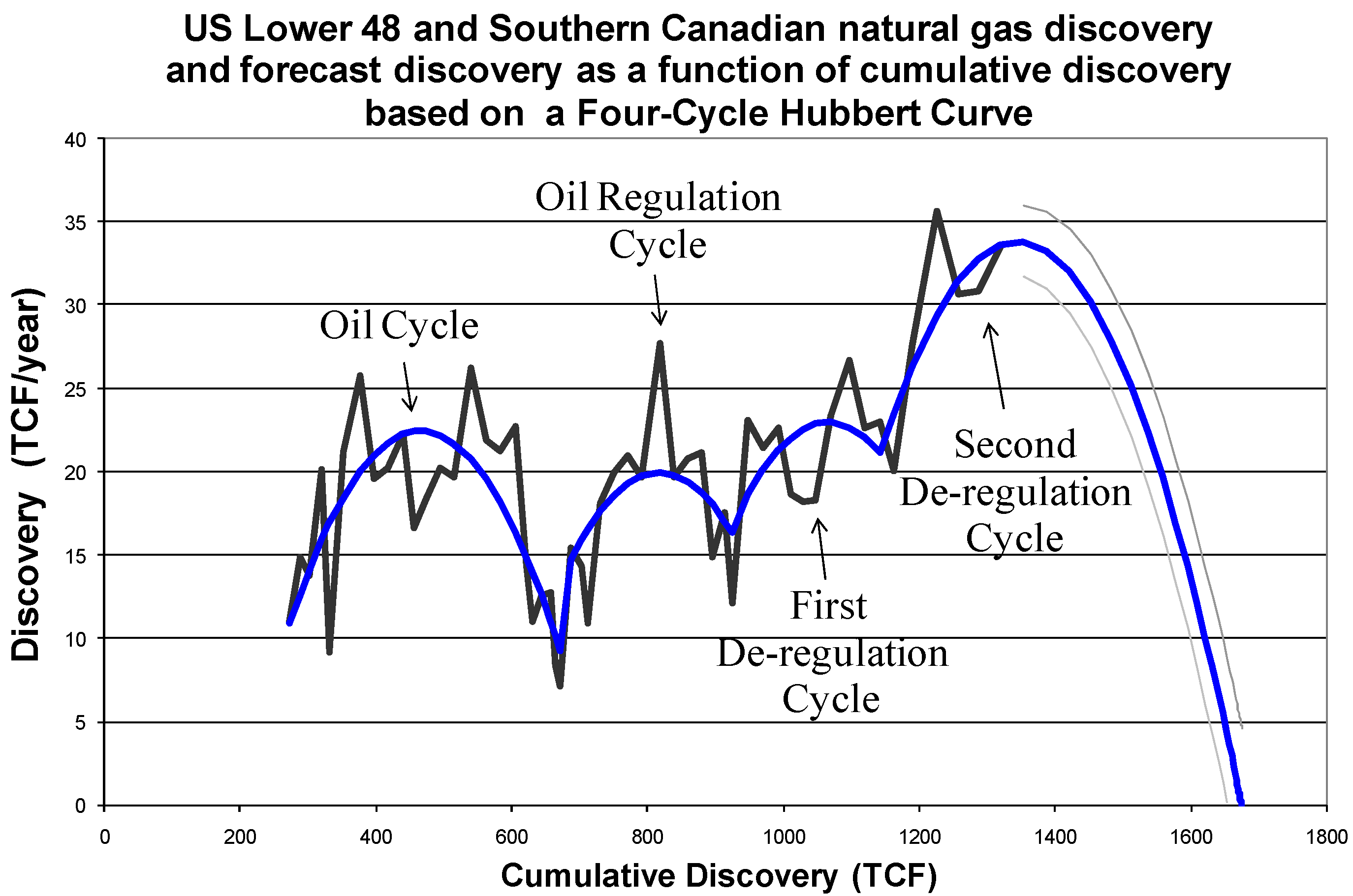
The estimated URR for the U.S. Lower 48 and Southern Canada only using data up to 2003 is 1676 trillion cubic feet of gas, with a 95% confidence interval between 1654 and 1698 trillion cubic feet. In other words, the data suggests that there is a greater than 97% chance that URR is less than 1700 TCF in the currently accessible regions for the first four Hubbert cycles. Below, we run a regression for data beyond 2003 with a fifth Hubbert cycle, but because another major change in price expectations occurred in 2005, there is not a long enough data set to be statistically confident about what the fifth Hubbert cycle will look like. Nevertheless, a simple forecast is made below.

Figure 3. Four Cycle Hubbert Curve.

Figure 3. Four Cycle Hubbert Curve.

Table 7. Test of Unit Root.

Null Hypothesis: RESIDUAL has a unit root
Lag Length: 0 (Automatic based on SIC, MAXLAG=10)
Exogenous: Constant
		t-Statistic	Prob.*
Augmented Dickey-Fuller test statistic		-6.786332	0.0000
Test critical values:	1% level	-5.416
	5% level	-4.7
	10% level	-4.348
*MacKinnon (1996) one-sided p-values.

Table 7. Test of Unit Root.

Null Hypothesis: RESIDUAL has a unit root
Lag Length: 0 (Automatic based on SIC, MAXLAG=10)
Exogenous: Constant
		t-Statistic	Prob.*
Augmented Dickey-Fuller test statistic		-6.786332	0.0000
Test critical values:	1% level	-5.416
	5% level	-4.7
	10% level	-4.348
*MacKinnon (1996) one-sided p-values.

The Figure 3, Table 6, four-cycle Hubbert model forecasts the natural gas URR, mostly from conventional but not shale natural gas sources, at 1700 TCF for the U.S. Lower 48 and Southern Canada. Compare this with an estimated URR of 1900 trillion cubic feet of conventional natural gas plus deepwater gas excluding Alaskan reserves that the U.S. Geological Survey [76] (USGS) forecast in 1995 for the United States. If we take that number and add 124 TCF of Canadian cumulative production and add 60 TCF of Canadian conventional reserves, then we get an estimated URR of 2084 TCF for the United States and southern Canada for conventional natural gas. This does not include expected extensions of proven reserves and expected discoveries of new fields in Canada’s southern region. Nevertheless, the four-cycle Hubbert URR of Figure 3 does look similar to the USGS forecast, although with a 26% lower estimate.

Note however, the four-cycle Hubbert curve of Figure 3 does not include conventional restricted reserves in Colorado and outer continental shelf (OCS) that may add an additional 200 TCF, which would make the USGS estimate and Figure 3 close. At this point though, restricted reserves may not postpone the projected peak in natural gas production but merely slow the post-peak decline.

9. Price Effects on the Hubbert Multi-Cycle

Before we can move on, we must test for the significance of price effects. Since economics suggests that price should be the cause of all supply phenomena, we check for its effect on the natural gas discovery trend. Recall above, we suggest that as long is price is above a threshold, its effect on supply is marginally small, i.e. relatively inelastic. Nevertheless, most economists believe price effects to be large, i.e. relatively elastic. So once the natural gas discovery pattern is de-trended, it is possible to see how prices affect discovery above or below the trend. First the percent change in price is compared to the percent change in production after it has been de-trended using Equation 5. Table 8 and Table 9 show the effects of the percent change in price on the percent change in the de-trended discovery. Two prices are looked at including the percent change in the current price (PCPR0), and the percent change in an average of a one and two year lagged prices (PCPR12), the latter being a possible indicator of future price expectations. Neither shows any significance.

Table 8. Detrended Discovery.

Dependent Variable: Detrended Discovery
Method: Least Squares
Sample (adjusted): 1951 2003
Included observations: 53 after adjustments
Variable	Coefficient		Std. Error		t-Statistic		Prob.
C	-0.040188		0.042086		-0.954904		0.3441
Per Cent Change in Price	0.000296		0.002290		0.129388		0.8976
R-squared		0.000328		Mean dependent var		-0.038431
Adjusted R-squared		-0.019273		S.D. dependent var		0.287248
S.E. of regression		0.290003		Akaike info criterion		0.399157
Sum squared resid		4.289199		Schwarz criterion		0.473507
Log likelihood		-8.577655		F-statistic		0.016741
Durbin-Watson stat		2.858432		Prob(F-statistic)		0.897560

Table 8. Detrended Discovery.

Dependent Variable: Detrended Discovery
Method: Least Squares
Sample (adjusted): 1951 2003
Included observations: 53 after adjustments
Variable	Coefficient		Std. Error		t-Statistic		Prob.
C	-0.040188		0.042086		-0.954904		0.3441
Per Cent Change in Price	0.000296		0.002290		0.129388		0.8976
R-squared		0.000328		Mean dependent var		-0.038431
Adjusted R-squared		-0.019273		S.D. dependent var		0.287248
S.E. of regression		0.290003		Akaike info criterion		0.399157
Sum squared resid		4.289199		Schwarz criterion		0.473507
Log likelihood		-8.577655		F-statistic		0.016741
Durbin-Watson stat		2.858432		Prob(F-statistic)		0.897560

Table 9. Detrended Discovery with lags.

Dependent Variable: Detrended Discovery
Method: Least Squares
Sample (adjusted): 1951 2003
Included observations: 51 after adjustments
Variable	Coefficient		Std. Error		t-Statistic		Prob.
C	-0.032290		0.044585		-0.724231		0.4724
Average per cent change in price, lags 1 and 2	-0.001293		0.003289		-0.393277		0.6958
R-squared		0.003147		Mean dependent var		-0.039084
Adjusted R-squared		-0.017197		S.D. dependent var		0.291033
S.E. of regression		0.293525		Akaike info criterion		0.424717
Sum squared resid		4.221683		Schwarz criterion		0.500475
Log likelihood		-8.830278		F-statistic		0.154667
Durbin-Watson stat		2.822783		Prob(F-statistic)		0.695821

Table 9. Detrended Discovery with lags.

Dependent Variable: Detrended Discovery
Method: Least Squares
Sample (adjusted): 1951 2003
Included observations: 51 after adjustments
Variable	Coefficient		Std. Error		t-Statistic		Prob.
C	-0.032290		0.044585		-0.724231		0.4724
Average per cent change in price, lags 1 and 2	-0.001293		0.003289		-0.393277		0.6958
R-squared		0.003147		Mean dependent var		-0.039084
Adjusted R-squared		-0.017197		S.D. dependent var		0.291033
S.E. of regression		0.293525		Akaike info criterion		0.424717
Sum squared resid		4.221683		Schwarz criterion		0.500475
Log likelihood		-8.830278		F-statistic		0.154667
Durbin-Watson stat		2.822783		Prob(F-statistic)		0.695821

Table 10. Hubbert curve with price instead of Indicator Variable.

Dependent Variable: Discovery
Method: Least Squares
Sample (adjusted): 1951 2003
Included observations: 54 after adjustments
Variable	Coefficient		Std. Error		t-Statistic		Prob.
C	1.709939		7.106074		0.240631		0.8109
CQD	0.063999		0.026211		2.441643		0.0185
CQD^2	-7.40E-05		2.46E-05		-3.013717		0.0042
PRICE	5.079707		1.186377		4.281698		0.0001
DUM88	-82.44584		30.89720		-2.668392		0.0105
DUM88*CQD	0.101482		0.033427		3.035962		0.0039
DUM98	-15.60761		46.20748		-0.337772		0.7371
DUM98*CQD	0.015013		0.039134		0.383638		0.7030
R-squared		0.614061		Mean dependent var		19.64048
Adjusted R-squared		0.555332		S.D. dependent var		6.144504
S.E. of regression		4.097368		Akaike info criterion		5.794520
Sum squared resid		772.2676		Schwarz criterion		6.089185
Log likelihood		-148.4521		F-statistic		10.45570
Durbin-Watson stat		1.631885		Prob(F-statistic)		0.000000

Table 10. Hubbert curve with price instead of Indicator Variable.

Dependent Variable: Discovery
Method: Least Squares
Sample (adjusted): 1951 2003
Included observations: 54 after adjustments
Variable	Coefficient		Std. Error		t-Statistic		Prob.
C	1.709939		7.106074		0.240631		0.8109
CQD	0.063999		0.026211		2.441643		0.0185
CQD^2	-7.40E-05		2.46E-05		-3.013717		0.0042
PRICE	5.079707		1.186377		4.281698		0.0001
DUM88	-82.44584		30.89720		-2.668392		0.0105
DUM88*CQD	0.101482		0.033427		3.035962		0.0039
DUM98	-15.60761		46.20748		-0.337772		0.7371
DUM98*CQD	0.015013		0.039134		0.383638		0.7030
R-squared		0.614061		Mean dependent var		19.64048
Adjusted R-squared		0.555332		S.D. dependent var		6.144504
S.E. of regression		4.097368		Akaike info criterion		5.794520
Sum squared resid		772.2676		Schwarz criterion		6.089185
Log likelihood		-148.4521		F-statistic		10.45570
Durbin-Watson stat		1.631885		Prob(F-statistic)		0.000000

Another criticism of the Table 6 model is that since the first indicator variable occurs in 1974, just when oil and natural gas prices increased, then a price variable can be inserted in place of the two 1974 indicator variables to see if a single price variable is the cause of the multi-cycle trend. We do this. The results are shown in Table 10. The Table 10 model does indicate that a price variable can adequately explain the discovery trend and have good statistical properties, however, its statistical properties are not nearly as good as the three indicator variable model of Table 6. The R² and the log likelihood of Table 10 are lower than that of Table 6. See Table 11.

Table 11. Comparison of Four versus Three Cycle Hubbert curve.

Model:	R2	Log Likelihood
Price plus two indicator Variables (1988, 1998)	0.614	-148
Three indicator Variables (1974, 1988, 1998)	0.713	-141

Table 11. Comparison of Four versus Three Cycle Hubbert curve.

Model:	R2	Log Likelihood
Price plus two indicator Variables (1988, 1998)	0.614	-148
Three indicator Variables (1974, 1988, 1998)	0.713	-141

However, just because natural gas prices increased in 1973 and stayed high does not mean the discovery rate trend would necessarily have changed. After all, oil and gas producers may have assumed that the 1973 price shocks were only temporary, in which case they would have exhibited only a slight deviation from the existing trend.

Normally in the oil industry, in order for price to create a change in exploration activities, explorers would have to be very sure that the new price will remain in effect. This has to do with expectations. A high price allows firms to begin to look for natural gas in high cost areas or in areas that were previously thought to be uneconomic, but that is only true if you believe that prices will stay high for many years. Note, exploring for and developing new natural gas reserves often takes ten years, and the resulting production activity will likely last for 30 years. If the explorer believes prices will spike suddenly and then just as quickly go back down, then there is no incentive for explorers to waste money exploring for more natural gas. However, a change in price expectations is different. A price expectation change could cause a change in the trend. The 1974 change in trend must then have been caused by a more powerful force than mere prices alone—it had to be an expectation change, not a simple price change.

A Newsweek article in December of 1973, Newsweek [69] states, “It will be years before new wells and more refineries can bring more oil to market. In the meantime America probably faces several years of chronic fuel shortages.” In other words, it was not oil and gas prices alone that changed in late 1973. Rather it was all future expectations about the value of oil that changed. Since natural gas is a good substitute for oil especially for electric power production and heating, this suggests that expectations for natural gas prices also changed. Based on expectations, then, the better variable for determining a change in trend is an indicatory variable, not a price variable. The 1974 indicator variable is an indication of price expectations. We know this indicator variable is powerful because it is the first indicator variable to emerge from the data.

10. Discussion of Indicator Variables and Institutions

In this section, we look to find the institutional changes that may have caused the indicator variables of Table 6. Looking back at the section on institutional economics it is argued that universal institutional changes are often the cause of changes in economic variables; although market specific institutions can also affect variables [36]. Looking at natural gas, it is easy to see that market specific variables are important. Natural gas is a particularly easy commodity to gain market control over, due to the need to transport it via pipelines, and therefore the natural gas market is vulnerable to a Rockefeller-type price manipulation. That is why the institutions regulating natural gas are so highly intrusive in comparison to institutions regulating, say, gold production. This justifies the idea that a specific commodity and its corresponding specific institutions must be analyzed in isolation from the rest of the economy and separately from market prices and costs. Institutions that affect the supply of metals won’t usually affect the supply of natural gas and vice versa. Thus we look at the natural gas institutions themselves.

For reasons of geology, physics and economics, the natural gas and crude oil industries have been intertwined. For oil, the supply market has always been straightforward: find oil, develop it, and sell it. This is due to the fact that oil is a relatively low cost commodity to transport, refine and store, such that it usually has been under a competitive market especially in the United States. But natural gas has not been under a particularly competitive market due to its relatively high cost of transportation.

Originally natural gas was found associated with oil and was considered a nuisance, which is why much of it was flared. Finally its value emerged as innovative marketing along with new technology for long distance pipelines made it saleable. But still it was linked to the search for oil and to a tightly regulated pipeline infrastructure rather than as its own stand-alone industry. Eventually though, the value of natural gas as an independent commodity emerged, especially in conjunction with electric power needs. The fact that oil and gas have been so closely intertwined, though, has made it difficult to estimate a supply of natural gas based on natural gas prices, natural gas costs and natural gas technology alone. This is why a close examination of natural gas market events is needed.

The Hubbert multi-cycle curve statistics show 1974, 1988, and 1998 are the best indicator variables for changes in the natural gas market. But the statistics do not tell us why these dates are important. This is what we explore here.

10.1. Indicator Variable #1, 1974

The demand for natural gas previous to 1974 was very low relative to natural gas reserves and therefore compared to potential supply. For example in the 1950s, reserves to production ratios were as high as 40 to 1 which means there was no reason whatsoever to have looked for more natural gas, yet more was found due to the search for oil. The regulatory institution in place was a highly intrusive Federal Power Commission (FPC) whose major concern was that a pipeline operator could create a monopoly over natural gas sales by buying out all of the interstate pipelines and limiting supply. So the FPC was the de facto planner for all new pipelines. Nevertheless, as restrictive as the FPC was, there was a slow increase in natural gas sales that gave oil producers a new profit center for their oil and gas activities. The FPC didn’t create an incentive to explore or develop natural gas as its own commodity, but it did at least allow for substantial development of natural gas, if it was found. However, the statistical evidence shows that something changed in 1974.

Two hypotheses attempt to explain the 1974 change in discovery rate. One hypothesis is that technological development related to natural gas reached a peak of advancement in 1972 [70]. Another hypothesis is that the 1978 natural gas policy act (NGPA) de-regulated natural gas pricing away from “vintage” prices—i.e. a regulated price that was determined by the point in time when natural gas was discovered—to a current price [41], and that the NGPA caused the change. However, neither hypothesis can totally explain events since they explain causes that either occur before or after the statistically relevant year of 1974; therefore, we look for another hypothesis.

An alternative hypothesis is that there emerged a new interest in finding natural gas and oil due to higher energy prices in general after 1973. Thus, one reason why the 1974 indicator variable works is because there was a price expectation change then. As explained above in the Newsweek quote, 1974 marked a change in expectations. A change in price expectations is a more powerful force for changing a discovery trend than a mere change in price. Still pipelines to deliver the natural gas could not be built very quickly due to continued stringent pipeline regulations, so the main factor in the change in the rate of discoveries of natural gas in 1974 goes back to the oil market.

Before 1973, oil prices were mostly unregulated, but in August of 1973 the Nixon Administration imposed a two-tier pricing system on all oil production, creating lower “old” oil prices and unregulated “new” oil prices. Then in February of 1976, the Energy Policy and Conservation Act came into effect creating further oil price regulations that lasted well into 1981. This oil regulation may have created an above-normal interest in finding “new” oil, ostensibly in deeper wells than where existing oil reserves occurred. However deeper oil wells usually locate mostly natural gas and very little oil, and therefore this push to find “new” oil undoubtedly translated inadvertently into finding much more natural gas. Therefore, the second cycle after 1974 is another oil related cycle and has more to do with oil institutions at the time than with natural gas institutions or even with natural gas price expectations.

10.2. Indicator Variable #2, 1988

After 1974, there was a clear need for cheap energy, thus we get back to the idea [38] that institutions change in reaction to outside influences just as much as they cause outside influences. That is institutions are endogenous. After 1974, calls to change American institutions on oil and gas were loud and clear, but it took awhile for the U.S. Congress to do anything about it and even longer for changes in law to have the desired effect. This brings up the next inflection point.

The next indicator variable we discover from the data can be found in 1988. However, 1988 does not look to be a year when any unusual institutional changes happened. The indicator variable could not be due to general natural gas deregulation at that time because much deregulation had already occurred previous to 1988, but not right at 1988 [44]. Natural gas deregulation started in 1978, with the NGPA, and there were major changes in rules in the early 1980s, as explained below, all of which means that 1988 surely could not have had anything at all to do with deregulation, that is unless deregulation was a longer process than just a mere change in the law. Usually in institutional economics it is assumed that a simple change in law and the consequences of that change happen all at once. However, in the U.S. and many other countries, like Russia [25], institutional changes can be more complicated than a mere change in the law or change in a constitution and therefore institutional changes occur slowly [71].

As mentioned above, efforts to deregulate natural gas started in 1978 when a new energy policy was passed by the U.S. Congress that included the Natural Gas Policy Act (NGPA) and the Fuel Use Act (FUA). Unfortunately the NGPA had incremental pricing and included a hodgepodge of previous regulations in some instances and no regulations in others so that it wasn’t true deregulation. In addition, the FUA ordered restricted gas use for many major utility uses. The market restrictions from these policies slowly melted away; nevertheless, truly free markets did not really appear until at least 1985 when spot market prices were introduced and when utilities were allowed free access to natural gas for any use. However, even then pipelines were still highly regulated which meant it was difficult to expand pipeline service to new supply areas or new demand areas which caused a lack of exploration efforts and there was still declining consumption. Clearly as of 1985, markets were still inhibited.

Then later in 1985, the U.S. Federal Energy Regulatory Commission (FERC) issued Order 436 creating pipeline unbundling. Unbundling meant that pipeline carriers and natural gas producers were separated from each other so that pipeline companies could no longer control gas producers, which in turn allowed greater competition to build pipelines and connect supply with demand. However a major court case from Order 436 was not decided until June 1987 which meant that Order 436 was not fully implemented until after 1987. FERC Order 500 codified changes subsequent to court cases in August 1987. Order 451, which ended price controls, was issued by the FERC in June of 1986, but a law dismantling all remaining incremental pricing wasn’t passed until May 1987. This suggests that it was not until 1988 when universal deregulation of prices and pipelines for the entire United States and Southern Canadian regions had been in place for a full calendar year. Note that Canada’s, and in particular Alberta’s, major customer was the United States and therefore even Canadian natural gas supplies were limited by American pipeline regulations. Thus 1988 has to be considered a crucial year in deregulation where a threshold of de-regulation was crossed making a permanent change in the market. This looks to be the reason that 1988 emerges from the data as the second inflection point for a multi-cycle curve.

Interestingly, natural gas consumption was also decreasing from 1984 to 1986 even though natural gas prices were decreasing and oil prices were still high, indicating that markets were not fully free. Finally in 1987 natural gas consumption started increasing, whereupon discovery picked up in the next year. This suggests that the 1985 natural gas law changed neither production nor discovery patterns until further court and legislative actions were implemented. It could be argued that other institutional or market effects during the mid to late 1980s could have caused a change in the natural gas discovery pattern such as changes in demand for energy in general or changes in general tax codes. But if this were true, we should see changes in coal and oil discovery, production or consumption patterns in the United States as well. A quick look at coal and oil shows no real change in their patterns. From 1984 to 1990 Lower 48 oil production declined smoothly. From 1984 to 1990, Lower 48 oil discovery generally decreased with some volatility. From 1984 to 1989, U.S. oil consumption increased smoothly until a slight dip occurred in 1990. From 1984 to 1990 U.S. coal consumption increased smoothly with one anomaly in 1986. From 1985 to 1990 coal production in the United States increased smoothly. Coal consumption in 1984 was slightly higher than 1985 but also substantially higher than 1983 making 1984 an anomaly above the smooth 1983 to 1990 trend. Finally coal discoveries are rarely affected by institutions at this point in time since U.S. coal reserves are so massive that there is very little incentive to search for more. In addition, during this period, the North American natural gas market was a closed market so that other world prices didn’t affect North America.

10.3. Indicator Variable #3, 1998

The next indicator variable occurs in 1998. Once again this is an odd time for an indicator variable. Better timing as far as exogenous market events were concerned would have been in 1993 just after the second round of natural gas deregulation. Actually, 1993, the first full year FERC Order 636 was implemented, was a second possibility for the third indicator variable, but not as good statistically as 1998. Oddly enough 1993 was not a close choice for a possible fourth indicator variable either. Nevertheless, there may be a reason why 1998 works as an indicator variable which again has to do with the further history of deregulation.

On April 8, 1992, the FERC issued Order 636 which pushed unbundling further by creating open access to pipelines. Order 636 allowed for the transition costs for unbundling to be charged, for the permitted rate structures to be redesigned, and for the voluntary capacity releases to be created. It also separated storage from transportation so that unbundling now included storage as well as producers, pipelines, and customers. Plus, Order 636 created secondary markets for all of these entities. However, one reason why 1998 may have become the dominant indicator variable rather than 1993 was because of legal concerns. FERC Order 636 delineated pipeline bundling as illegal after it had been allowed before. In other words, in the 1980s all new contracts had to be unbundled, but existing contracts with some pipelines and producers still bundled together was allowed. Now all existing bundling contracts became expressly illegal. By changing existing contracts from legal to illegal, suddenly a number of cases went to court over existing contracts [72,73]. Probably it was these court cases that delayed the full effect of Order 636 for years, not allowing full penetration of the market until 1998.

Another way to model the Multi-Cycle Hubbert curve is to put a dummy variable in 1993 and do an intervention model, where the effect of the dummy variable is nonlinear [74]. However, such a model is messy because it requires the use of a transfer function. However, the data suggests that there was a small spike between 1993 and 1995, then a decline, and the real surge occurred in 1998. Therefore, 1998 is shown to be the true inflection point for a multi-cycle Hubbert curve.

10.4. 2005 Expected Price Change

The data for the above statistical analysis that reveals the 1974, 1988 and 1998 indicator variables ends in 2003 because that is when natural gas price volatility started changing. However, the current trend in natural gas discovery and production appears to show that a new change in the natural gas market has occurred since 2005. In 2005, the expected price of oil as presented by the Energy Information Administration [75] suggests that another change in natural gas price expectations occurred. Due to a lack of data points after 2005, this new indicator variable and the additional fifth Hubbert cycle it created is not added to the original discovery analysis. However, this fourth indicator variable may be used to project a fifth Hubbert multi-cycle in order to forecast the Lower 48 natural gas supply as Hubbert did in 1956 for oil.

One of the changes in the natural gas supply market that the 2005 natural gas expected price increase created was that it made Devonian, Haynesville and Barnett shale natural gas feasible to exploit. Already in 2005 horizontal drilling technology and shale natural gas deposits were well recognized, but the expected price of natural gas was too low to feasibly exploit that technology on those deposits. After 2005, that changed. Thus it is important to estimate a new natural gas URR for the Lower 48 and Southern Canada with a fifth “price expectations” Hubbert cycle, which we do below.

10.5. Further Variables

The four market events shown above stand out as being statistically powerful enough to cause a change in the natural gas discovery trend. They are the oil price expectation shock of 1974, along with oil’s two tier pricing; the pipeline regulation changes in the 1980s culminating in 1988; the pipeline regulation changes in the 1990s culminating in 1998, and the price expectation change of 2005. We call the first Hubbert cycle the “oil” cycle, the second Hubbert cycle the “oil regulation” cycle, due to two tier oil pricing, the third Hubbert cycle the “first deregulation” cycle, the fourth Hubbert cycle the “second deregulation” cycle, and the fifth Hubbert cycle the “price expectations” cycle.

Other sets of institutions that may have affected natural gas markets are environmental regulations, such as the Clean Air Act of 1992, and electric power de-regulation which could have had an effect on the need for natural gas, which would then affect discovery. However, the demand for natural gas is determined by its price. Even if using natural gas became more attractive through legislative changes, the price would reflect that change, and as we have already seen, small price changes have very little effect on discovery and supply, and only two large price changes occurred, one in 1974 and one in 2005. Environmental policy may have affected where industry was allowed to look for natural gas, although no one single regulation had the power to create a large change in supplies. In addition, changes in tax policies are usually small enough not to affect the industry substantially in any one year. For example the windfall profits tax during the Carter Administration certainly would have affected oil, but not necessarily natural gas owing to the limited change in natural gas profitability. However, such taxes or environmental laws should have affected oil and coal as well but they didn’t. We are left with natural gas specific institutional changes as described above as the most likely cause of the inflection points.

11. The North American Natural Gas Production Forecast—Peak Gas

Already the years 2000, 2003, and 2005 have witnessed above average natural gas price increases up to and above $10 per MCF. A change in the EIA’s thirty year oil price forecast in 2005 [75], along with the witnessed natural gas price changes, strongly suggests a change in the expected future price of natural gas especially since oil and gas prices often follow a similar path due to substitution. The year 2005 has to be considered the initiating point of a fifth Hubbert multi-cycle where Barnett, Devonian and Haynesville Shale gas among others now look to be feasible to produce.

In order to give a forecast of supply, a five-cycle natural gas discovery Hubbert curve is estimated in Table 12. This is shown in Figure 4. Table 12, Figure 4, model uses data up until 2008, along with a new indicator variable in 2005 to create a simple OLS regression that signals the initiation of a fifth Hubbert cycle. The natural gas discovery forecast of Figure 4 is expected to reveal the true ultimately recoverable resource of the central North American natural gas region at about 2150 TCF. This forecast is not without controversy.

Table 12. Five Cycle Hubbert Curve Estimate.

Dependent Variable: QD (rate of Discovery, TCF/year)	Method: Least Squares	Sample (adjusted): 1950 2008	Included observations: 59 after adjustments
Variable	Coefficient	Std. Error	t-Statistic	Prob.
C	-45.4603	11.94264	-3.80655	0.0004
CQD	0.292579	0.052688	5.553024	0.0000
CQD^2	-0.00031	5.48E-05	-5.7364	0.0000
DUM74	-144.505	26.09661	-5.53733	0.0000
DUM74*CQD	0.221414	0.038736	5.716007	0.0000
DUM88	-144.198	33.74944	-4.27261	0.0001
DUM88*CQD	0.156407	0.03543	4.414479	0.0001
DUM98	-155.192	44.94822	-3.45267	0.0012
DUM98*CQD	0.138126	0.038546	3.583422	0.0008
DUM05	-373.362	66.67524	-5.59972	0.0000
DUM05*CQD	0.269746	0.048294	5.585535	0.0000
R-squared	0.801235	Mean dependent var	20.92674
Adjusted R-squared	0.759825	S.D. dependent var	7.866405
S.E. of regression	3.855137	Akaike info criterion	5.703235
Sum squared resid	713.3798	Schwarz criterion	6.090572
Log likelihood	-157.245	F-statistic	19.34911
Durbin-Watson stat	2.02837	Prob(F-statistic)	0.000000

Table 12. Five Cycle Hubbert Curve Estimate.

Dependent Variable: QD (rate of Discovery, TCF/year)	Method: Least Squares	Sample (adjusted): 1950 2008	Included observations: 59 after adjustments
Variable	Coefficient	Std. Error	t-Statistic	Prob.
C	-45.4603	11.94264	-3.80655	0.0004
CQD	0.292579	0.052688	5.553024	0.0000
CQD^2	-0.00031	5.48E-05	-5.7364	0.0000
DUM74	-144.505	26.09661	-5.53733	0.0000
DUM74*CQD	0.221414	0.038736	5.716007	0.0000
DUM88	-144.198	33.74944	-4.27261	0.0001
DUM88*CQD	0.156407	0.03543	4.414479	0.0001
DUM98	-155.192	44.94822	-3.45267	0.0012
DUM98*CQD	0.138126	0.038546	3.583422	0.0008
DUM05	-373.362	66.67524	-5.59972	0.0000
DUM05*CQD	0.269746	0.048294	5.585535	0.0000
R-squared	0.801235	Mean dependent var	20.92674
Adjusted R-squared	0.759825	S.D. dependent var	7.866405
S.E. of regression	3.855137	Akaike info criterion	5.703235
Sum squared resid	713.3798	Schwarz criterion	6.090572
Log likelihood	-157.245	F-statistic	19.34911
Durbin-Watson stat	2.02837	Prob(F-statistic)	0.000000

Figure 4. Five Cycle Hubbert curve.

Figure 4. Five Cycle Hubbert curve.

The first, and most important, criticism of Table 12, Figure 4 Hubbert forecast is that the fifth Hubbert curve natural gas discovery cycle does not yet have enough data points to make such a forecast possible. With only three data points since 2005, anything can happen. The forecast as it is laid out depends on similar characteristics of the fifth cycle as occurred in the preceding four cycles, but those characteristics may be quite different; therefore, it’s too early to do a forecast. Hubbert’s original forecast was subject to the same criticism—off-shore and new regions will act differently than in the past. This forecast gets the added criticism that we are going into shale natural gas, which is so fundamentally different from conventional natural gas that the fifth Hubbert cycle will not match at all the previous cycles. Yet, even though the physical structure of the geology below the earth is different for shale natural gas than for conventional natural gas, nevertheless the business mechanics of the search process are similar: look for natural gas where you are most likely to find it, develop the most easily exploitable reserves first, and make a ruckus about speculative reserves in order to get investors interested.

Another criticism of the Table 12, Figure 4 Hubbert forecast may be that it was not a simple price change that is creating the fifth Hubbert cycle but rather a technology change. However, as suggested above, the primary technologies for shale natural gas already existed. Nevertheless, these technologies are being touted exuberantly as being able to unlocked reserves of natural gas so vast that natural gas supplies will last for decades [26]. However, as in Hubbert’s day with regard to oil, the shale gas reserves of the United States may be less than anticipated.

Note that Barnett shale natural gas production using horizontal drilling in the Fort Worth, Texas, area has increased by an average of 125% per year for four years [27]. This is reminiscent not of a typical Hubbert curve for oil and gas production when new reserves are unknown, such as in the U.S. or Russia in the early 20^th century when oil and gas production increased by at most 10% per year, but rather a production curve where reserves are well known. When reserves are well known such as when the trans-Alaska oil pipeline opened in 1977, 8 years following the discovery of the great Prudhoe Bay oil field and thus where explorers had had a full 8 years to delineate and develop the field before actual production could commence, production can increase fast. In fact, in the Prudhoe case, oil production increased by an average of 100% per year for four years until it reached the maximum output and plateaued.

Similarly since Barnett shale natural gas production has been expanding so quickly, this suggests that much was already known about those reserves before production increased. It took a price change to make the shale natural gas production feasible, but the quick production rise suggests that a production limit will quickly be reached. Quick increases in oil and gas production, like what has happened in the Barnett shale basin, can just as quickly plateau. We therefore speculate that much of the new natural gas shale resources, such as Devonian, Haynesville and New Albany shale, will likewise quickly reach limits of production, where the very large stock of reserves will be subject to limited rates of production flow.

Assuming the five-cycle Hubbert discovery curve of Figure 4 is correct, a URR of 2150 TCF is used to forecast the Lower 48 and Southern Canadian natural gas production. From that URR the quadratic Hubbert curve for production, derived from above, is given as:

QP = a*CQP – (a/URR)*CQP²

(7)

Using early natural gas production data, the initial rate of increase of North American natural gas production is 8.1%, which is used for the “a” parameter. This was calculated by fitting the model to data between 1950 and 1973 using nonlinear regression with the Levenberg-Marquardt algorithm in SAS. By substituting the estimated URR of 2150 TCF from Figure 4 and the 8.1% initial rate, then North America could have a supply shortfall by 2013. A shortfall is defined when the maximum production level goes below the recent upward trend in demand, which has been 7% per year over the last three years. See Figure 5.

Figure 5. Forecast Consumption.

Figure 5. Forecast Consumption.

Figure 6 shows the same curve but as a function of time where the current consumption is forecast and the expected supply peak is shown. By 2013, North American natural gas production may peak and prices should rise possibly higher than one tenth the per barrel price of oil that is typical for natural gas depending on how quickly oil substitutions can be made and on how much substitution is possible. Usually natural gas is priced at $5 per thousand cubic feet whenever oil is priced at $50 per barrel, but lately natural gas is as low as $3 per thousand cubic feet even though oil is above $50 per barrel. After 2013, we may see a substantial rise in natural gas prices, if peak natural gas occurs.

Figure 6. (a) Forecast consumption over time.

Figure 6. (a) Forecast consumption over time.

A natural gas supply shortfall with oil substitution could push oil prices to spike higher than they were in 2008, creating an amplifying effect on oil prices. Note, that three billion cubic feet (BCF) of natural gas production per day (equivalent to one trillion cubic feet (TCF) per year) is the same amount of energy as 0.5 million barrels of oil a day. So if US natural gas production declines by two TCF per year, we will need an additional one million barrels of oil a day to compensate. By 2020, it is possible to have a 20 TCF per year natural gas shortfall, causing the US to need an additional 10 million barrels of oil a day on top of its anticipated 25 million barrels of oil a day consumption, assuming imports of LNG cannot compensate for the US natural gas shortfall.

Notice in Figure 6 the sharp the rise and fall of natural gas production for the forecast consumption and forecast supply scenario. It is unusual for production to be able to peak and decline so sharply, and since the large stock of shale resources will have a limited flow rate of production, peak natural gas may occur at a lower level and later, then exhibit a slower decline rate. Therefore, an alternative forecast is shown in Figure 6 that peaks in 2015, but where a slowdown in production starts in 2010.

12. The Strategic Natural Gas Market

The forecast shortfall between projected North American consumption and supplies will become more severe if natural gas is used as a substitute for oil. According to industrial surveys, most of the fuel switching between oil and natural gas for power production already happened as of 2000 [77]. The current fuel-switching capacity is 5-10% of industrial demand, but only between natural gas and oil. Natural gas demand in the power sector may increase as a result of new planned combined-cycle electrical power generators to take the place of coal generators. The business as usual forecast means an additional 5 BCF a day of natural gas will be needed for new electric power plants by 2013 [78]. That demand surge may not materialize if there is a continuing recession; nevertheless, it means that the natural gas market will be getting tight in the coming years because of the need for electricity and the reluctance for coal fired power. A natural gas crisis could hit North America sometime after 2010, but would soon spread to Europe and elsewhere as North America competes for liquefied natural gas (LNG) with the rest of the world.

LNG can be shipped around the world. Since regasification facilities and LNG tankers far outnumber liquefaction facilities [79], supply markets have become liquid. Natural gas prices are on the verge of becoming unified around the world, although with some regional price differentials owing to tariffs reflecting regional distances as well as supply bottlenecks. As of 2009, the price of a natural gas is significantly lower on the Atlantic Basin than on the Pacific Rim but that could change if North American natural gas supplies peak in 2013 or rise more slowly starting in 2010 as Figure 6 suggests.

Even though a North American recession continues, natural gas consumption can easily climb steadily and force North America to start buying LNG on the open market by 2010. Since regasification facilities outnumber liquefaction facilities a highly competitive LNG market may emerge. Qatar is the key.

While Russia has much more natural gas than Qatar, the Siberian energy superpower has a fixed supply route to a large natural gas customer: Western Europe. And while Russia can play games with European supply, Qatar will simply satiate the highest netback priced market. (The netback price is the price of the natural gas at its source location: $5 Henry Hub price minus $3 tariff for shipping to the U.S. equals $2 netback price at Qatar.) If the Pacific Rim gives Qatar the highest netback price, then Qatar will sell there; if the Atlantic Basin gives Qatar the highest netback price, then it will sell there. Note, Qatar is 6,480 nautical miles from Japan, but only 3,307 miles from Portugal, and 1,290 miles from India. However, Qatar is 9,687 miles to the U.S. Gulf Coast, where the Henry Hub is. Since North America is farther from Qatar than Japan, then the equalization of the netback prices to Qatar suggests that in fact the Atlantic Basin will in the future have the higher natural gas price compared to the Pacific Rim. Currently, because of North American supplies, the Atlantic Basin has cheaper natural gas than the Pacific Rim, but the market difference will change, quite possibly abruptly, when North American natural gas supplies peak. Because of substantial Gulf Coast storage capacity, North America may be able to buy low priced LNG during the summer and consume it in winter, mitigating high prices to a degree.

13. Conclusions

While there is clear evidence that a conventional Hubbert curve doesn't work in a number of regions, other evidence shows that a Hubbert curve does work especially under unfettered markets. What has been missing from the discussion is the role that institutions play in affecting the supply of oil and natural gas—any mineral resource.

What we find for the natural gas market is that there exist definite Hubbert curve-like characteristics for discovery. However, market specific institutions play a role. In particular, 1974, 1988 and 1998 look to be points in time where new institutions caused inflection points for a Hubbert multi-cycle natural gas discovery curve. Those institutional changes were not arbitrary; rather, they were reactions to the oil and gas market such as the high energy prices of the 1970s. The American natural gas market is marked by energy prices causing North America to embrace new institutions just as much as new institutions caused changes to the natural gas supply.

The change in institutions that occurred in America suggests that forecasting oil and gas supplies using a simple Hubbert curve without regard to institutional characteristics is unsound. This means that oil and gas forecasts may need to be revised to include institutions and expected changes in those institutions. Hubbert critics will revel in the fact that many an oil and gas producing country can de-regulate in order to increase world supplies. Hubbert supporters can take heart in the fact that the Hubbert curve works as long as institutional effects are accounted for. If evidence shows that a Hubbert curve does not work for a given region, that evidence must be analyzed in light of institutional economics before the Hubbert curve hypothesis can be rejected. However, a Hubbert curve that occurs within a region where the institutions allow for free markets and where a well adjudicated property rights system exists, such as occurred in the United States, could make a good test of the Hubbert curve hypothesis.

Hubbert curve analysis suggests that by having better institutions, it is possible to have greater supplies of oil and gas. However, if institutions are like technology, then energy producing countries can use the institutions or not use them or change them depending on how institutions benefit that particular country. In the case of America, free market institutions were optimal and maximized oil and natural gas value to the United States. In the case of Saudi Arabia, Russia or Mexico it might be the case that a different set of institutions are optimal and would maximize those countries values. Therefore, any given country may never reach a Hubbert curve type peak in production in the American tradition but rather have a long plateau of production well under its Hubbert curve potential. It also may mean that the world oil and gas production may consistently stay below a U.S. style Hubbert curve supply. A simple Hubbert curve may be optimistic.

In the medium term, natural gas supplies in central North America may look substantial [80], but they may soon peak and cause a tremendous switch from North American natural gas self sufficiency to North American natural gas supply shortfalls. If that happens then LNG imports into the United States could force the Atlantic Basin LNG price to climb higher than the Pacific Rim price and add to a general worldwide oil and natural gas energy crisis.
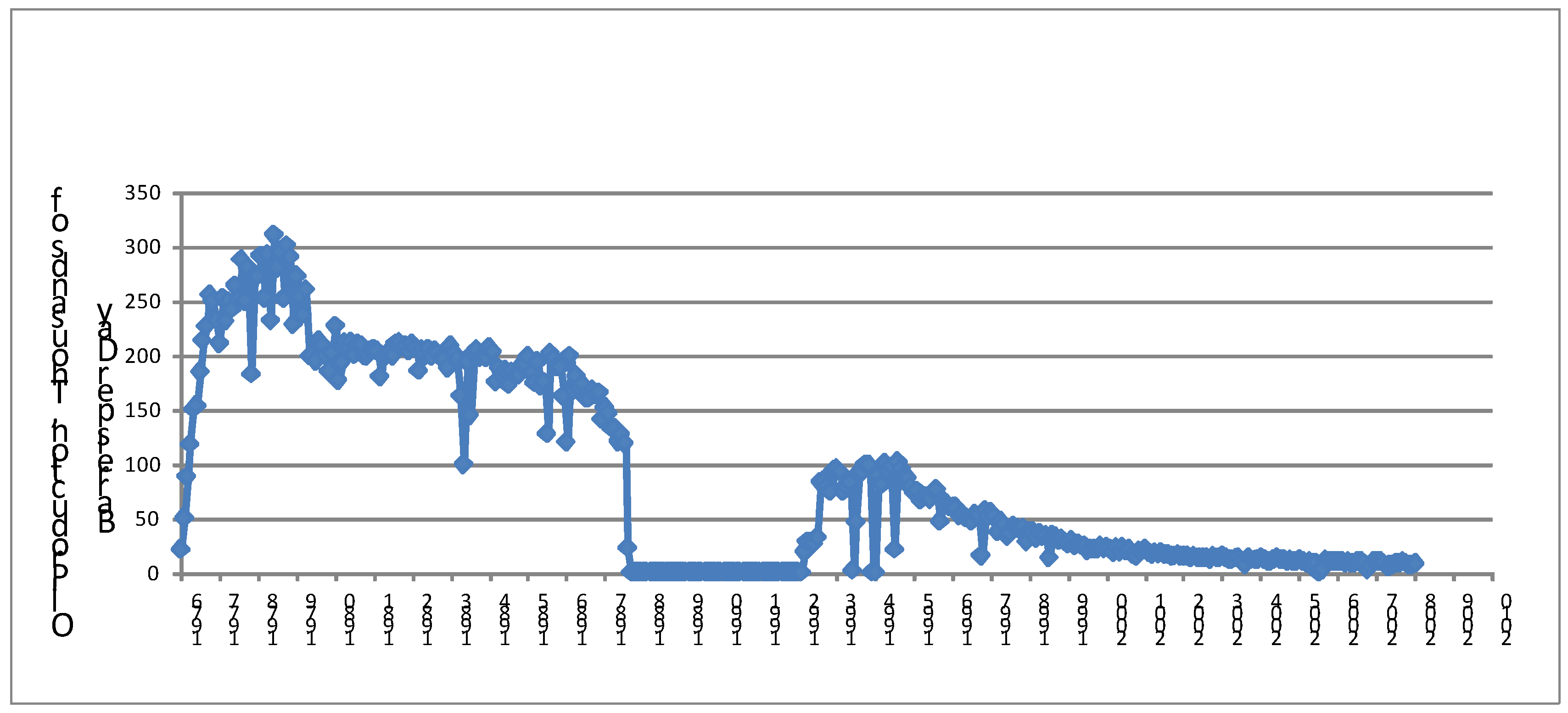
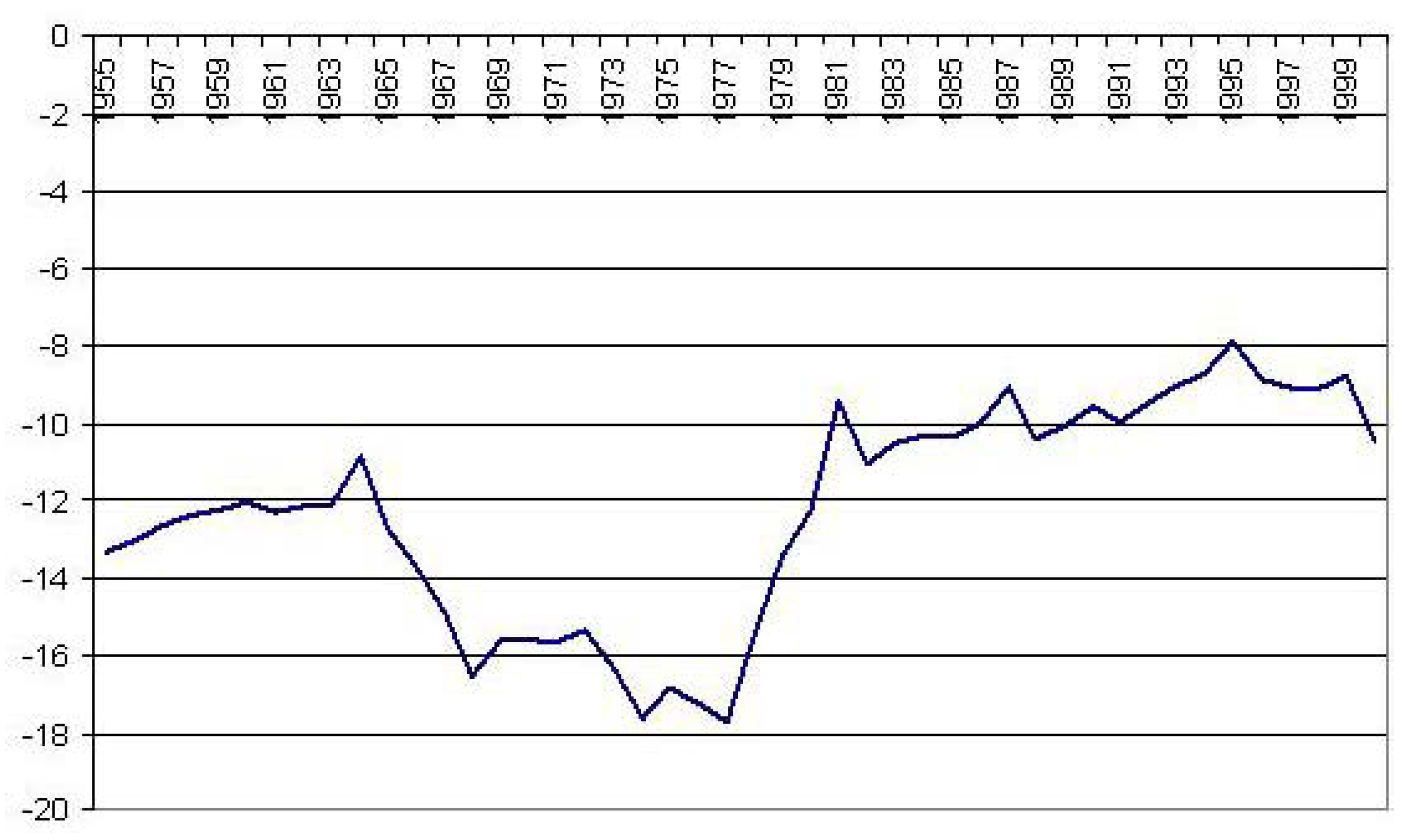
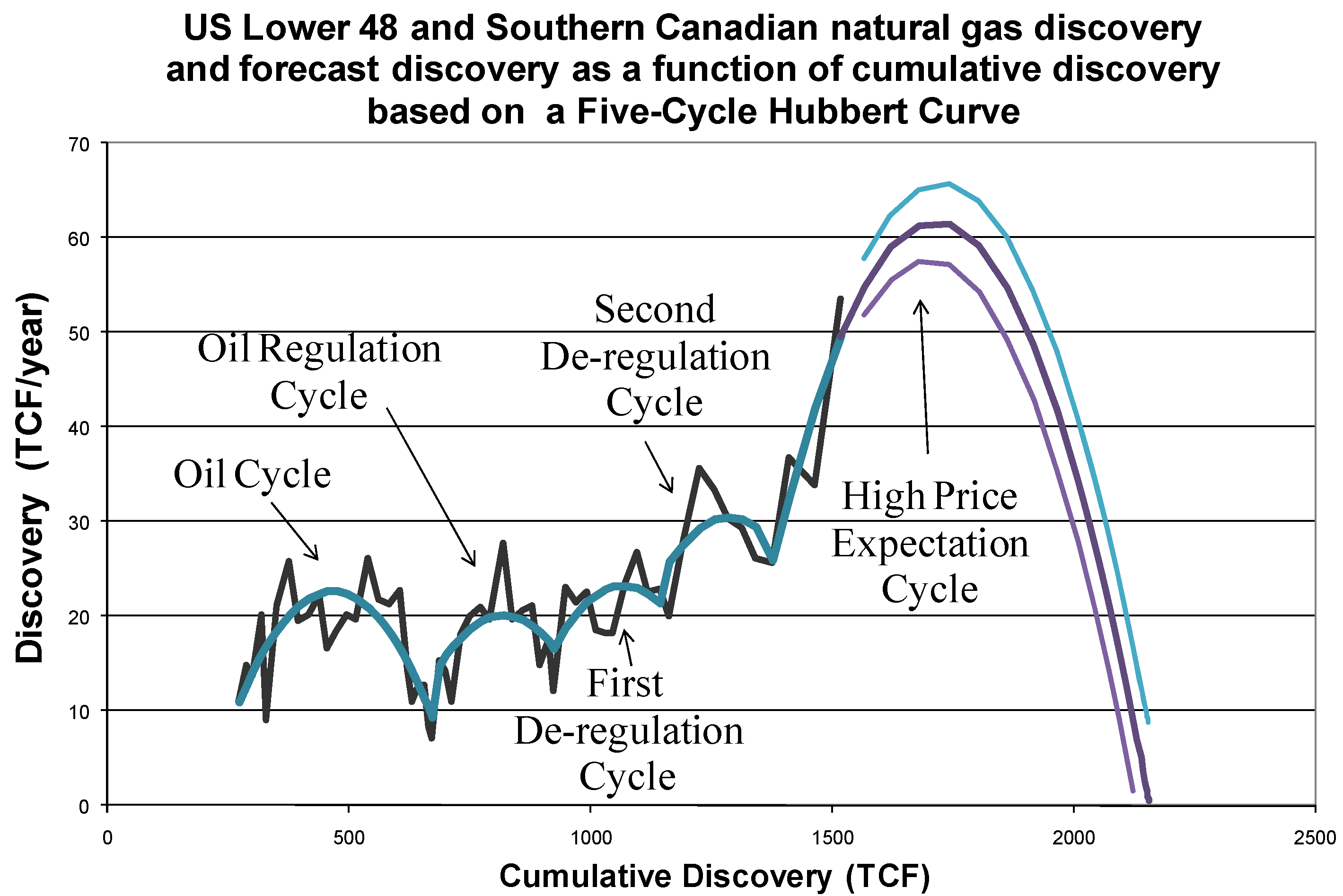
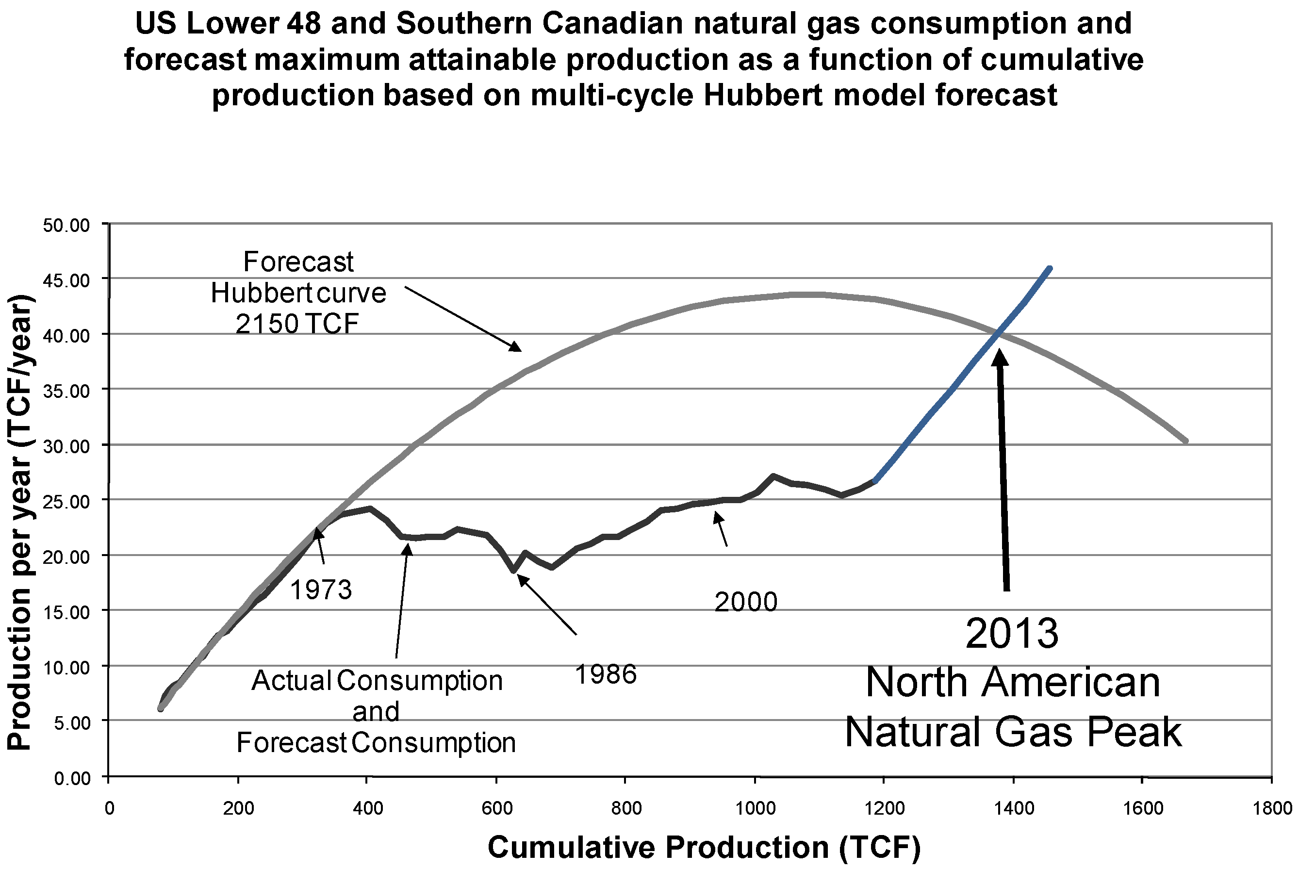