A Novel Technique to Determine Concentration-Dependent Solvent Dispersion in Vapex

Abstract

Vapex (vapor extraction of heavy oil and bitumen) is a promising recovery technology because it consumes low energy, and is very environmentally-friendly. The dispersion of solvents into heavy oil and bitumen is a crucial transport property governing Vapex. The accurate determination of solvent dispersion in Vapex is essential to effectively predict the amount and time scale of oil recovery as well to optimize the field operations. In this work, a novel technique is developed to experimentally determine the concentration-dependent dispersion coefficient of a solvent in Vapex process. The principles of variational calculus are utilized in conjunction with a mass transfer model of the experimental Vapex process. A computational algorithm is developed to optimally compute solvent dispersion as a function of its concentration in heavy oil. The developed technique is applied to Vapex utilizing propane as a solvent. The results show that dispersion of propane is a unimodal function of its concentration in bitumen.

1. Introduction

The enormous heavy oil and bitumen deposits in the World are estimated to be approximately 6 trillion barrels [1]. Canada and Venezuela have the major parts of these resources. These huge reserves are so attractive that many attempts have been made to invent numerous schemes to recover these heavy oil and bitumen resources. In Canada, steam-based methods are often employed to improve heavy oil recovery by reducing the viscosity of in-situ heavy oil. However, these methods are ineffective and uneconomical for reservoirs with thin pay zones, underlying bottom water, overlying gas caps, low rock conductivities, and high water saturations [2]. On the other hand, solvent based methods provide a better alternative for heavy oil recovery that can eliminate several problems associated with steam based methods such as water and energy requirements, emissions of greenhouse gases and wastewater generation [3]. Vapex is one of the most promising heavy oil solvent based recovery methods [4].

In Vapex, vaporized solvents at pressures close to dew point are injected into a heavy oil reservoir through an upper horizontal well to reduce the viscosity of the native heavy oil. The diluted oil flows to the lower horizontal well under the action of gravity. The transport mechanism involved in Vapex is dispersion, i.e. the combination of molecular diffusion of solvent into the heavy oil, and its convection under the action of gravity aided by viscosity reduction, concentration gradient, and capillary action. Live oil mobility and its convection are also influenced by the action of gravity and surface renewal [3]. Investigators had to use dispersion coefficients that are up to four orders of magnitudes higher than the diffusion coefficients in order to predict the actual production rates [5,6,7,8]. Solvent dispersion is the reason for the high oil production rates in porous media. The movement of solvent in a porous medium is facilitated by convection, and the mass transfer is higher than that due to diffusion alone [9].

Oil production in Vapex depends on the viscosity of live oil, i.e. the liquid phase consisting of solvent and heavy oil. This viscosity influences the movement of the live oil in the reservoir. The solvent concentration within the heavy oil depends on the thermodynamic properties of the solvent, operating conditions, and solvent dispersion in the heavy oil. According to Upreti et al. [4] accurate concentration-dependent dispersion data for solvent-heavy oil and bitumen systems are necessary to determine:

• The amount and flow rate of solvent required to mobilize the heavy oil.
• The extent of heavy oil and bitumen reserves that would undergo viscosity reduction.
• The time required to mobilize the heavy oil and bitumen for drainage under gravity.
• The production rate of live oil.

A few studies exist on the determination of dispersion of various solvents used in Vapex. Boustani and Maini [10] have shown a strong concentration dependence of dispersion, as observed in the case of molecular diffusion by Upreti and Mehrotra [11,12]. Kapadia et al. [7] developed and simulated a mathematical model with a linear concentration-dependent dispersion to determine gas dispersion during the vapor extraction of Cold Lake bitumen from a rectangular block of homogeneous porous medium using butane. The dispersion coefficient was found to be four orders of magnitude higher than reported molecular diffusion. Using a linear dispersion model, El-Haj et al. [8] conducted Vapex experiments, which were simulated by a mathematical model to determine the dispersion coefficient of butane gas into Athabasca bitumen. The dispersion coefficient obtained was two to three orders of magnitude higher than molecular diffusivity reported earlier.

The above findings coupled with the paucity of dispersion data in the literature make it imperative to determine the concentration-dependent dispersion for various solvents in heavy oil and bitumen. For this purpose, we have developed a new technique which is based on variational calculus. The salient feature of this technique is that it does not impose any functional form on dispersion as a function of concentration, but allows its realistic determination.

2. Experimental Setup

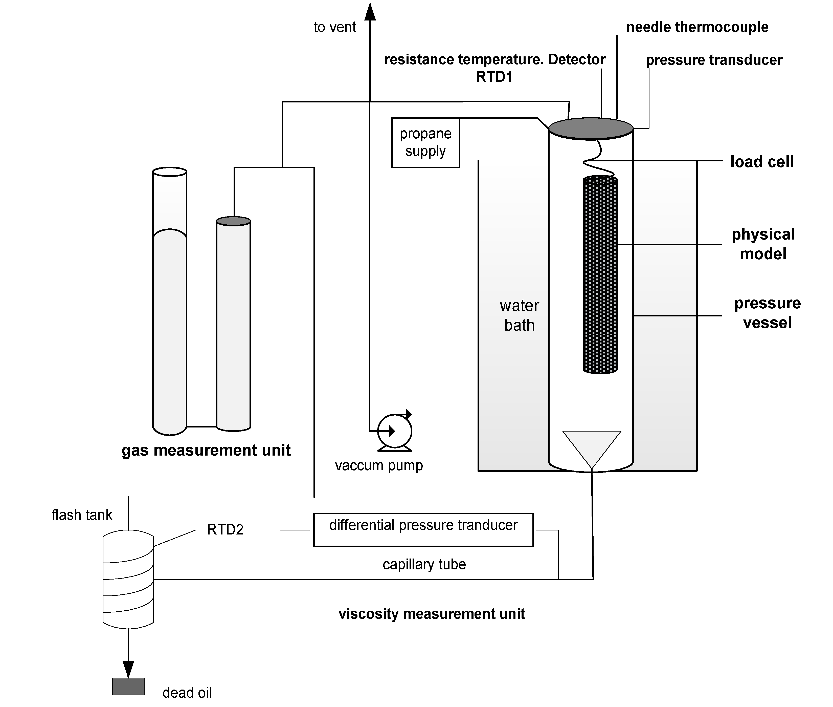
Figure 1 shows the schematic diagram of the experimental setup used. The setup comprises of a cylindrical pressure vessel of 55 cm height and 15 cm internal diameter inside a temperature-controlled water bath.

Figure 1. Schematic diagram of the experimental setup.

Figure 1. Schematic diagram of the experimental setup.

The vessel holds the physical model of Vapex. The physical model comprises a cylindrical wire mesh filled with glass beads saturated with heavy oil. The physical model is suspended from a load cell, and kept in contact with the solvent vapor at constant pressure. The load cell records the mass of the physical model with time. The mass decreases in an experiment as live oil drains away from the model due to solvent absorption. The drained oil is directed to a calibrated 25 cm³ collection tube. The tube is connected to a viscosity measurement unit to measure the online live oil viscosity.

The viscosity measurement unit comprises a 50 cm long stainless steel capillary tube of 0.1016 cm internal diameter equipped with a differential pressure transducer. The capillary tube is connected to a stainless steel flash tank of 300 cm³ capacity. The flash tank is wrapped with an electrical heating tape. The volume of propane separated from the live oil inside the flash tank is measured by a gas measurement unit. It is composed of two cylinders of respective capacities 2,600 cm³ and 2,900 cm³. A needle thermocouple and two resistance temperature detectors respectively measure the temperature of the packed medium, propane gas, and the flash separation tank. A data acquisition system records the system properties online.

2.1. Experimental Procedure

A sample of heavy oil (from Imperial oil; of 200,000 mPa∙s viscosity, and 1,001 kg/m³ density at 22 °C) was heated to 60 °C. Glass beads of known permeability were gradually added to the heated heavy oil ensuring proper mixing without trapping air bubbles. The saturated mixture of the heavy oil and glass beads was packed into a cylindrical wire mesh of 25 cm height, and 6 cm diameter. During this operation, the mesh lay inside an ice bath to prevent the bitumen from oozing out. The cylindrical packed medium, i.e., the physical model of Vapex, of heavy oil saturated with glass beads was weighed, and left at room temperature for one day to reach thermal equilibrium prior to an experiment.

Before starting an experiment, the vessel was pressurized with air and left for 24 hrs to test any leaks. The physical model was suspended from the load cell inside the pressure vessel. Research grade propane of purity 99.99% was used. The vessel was flushed with propane of about twice its volume and vacuumed to −15 mmHg. Propane was injected into the vessel at constant pressure. The injection pressure was controlled through the pressure regulator installed on the supply propane cylinder. The water bath temperature was kept 1–2 °C higher than the dew point temperature of propane. The experiment was carried out for 5 hrs.

Propane upon being injected diffused into the physical model from its exposed outer surface. The heavy oil became less viscous and began to drain and produce as live oil. The load cell recorded the decrease in the mass of the physical model every minute as the oil production continued. The live oil was collected for the measurement of viscosity and flow rate. When about 15 cm³ of live oil was collected, the oil was drained through a capillary tube into the flash tank. The propane liberated from the live oil in the flash tank was directed to the gas-measurement unit filled initially with water. The displaced volume of water determined the propane volume. The propane-free oil residual in the flash tank was weighed. The amount of live oil produced with time was recorded.

Table 1 provides the experimental parameters and operating conditions.

Table 1. Experimental parameters and operating conditions.

Parameter	Value
permeability (K), Darcy	204
porosity (φ)	0.38
temperature,°C	21
pressure, MPa	0.689

Table 1. Experimental parameters and operating conditions.

Parameter	Value
permeability (K), Darcy	204
porosity (φ)	0.38
temperature,°C	21
pressure, MPa	0.689

3. Theoretical Development

The technique developed in this work relies on the mass transfer model of vapor extraction of heavy oil using a solvent. The model has an undetermined concentration-dependent dispersion function. Incorporating this function in the mass transfer model, the calculated mass of oil produced should be equal to its experimental value obtained from the experiments.

3.1. Mass Transfer Model

A mathematical model is developed here to describe the mass transfer process based on the vapor extraction experiments. The assumptions involved are as follows:

• Vapex is carried out at constant temperature and pressure.
• Solvent dispersion is along the radial direction only.
• The velocity of the live oil along the vertical direction is governed by Darcy law in a porous medium.
• The porous medium has uniform porosity and permeability.
• There are no chemical reactions.
• Any volume change results and corresponds to drainage of the live oil.
• The heavy oil is non-volatile.

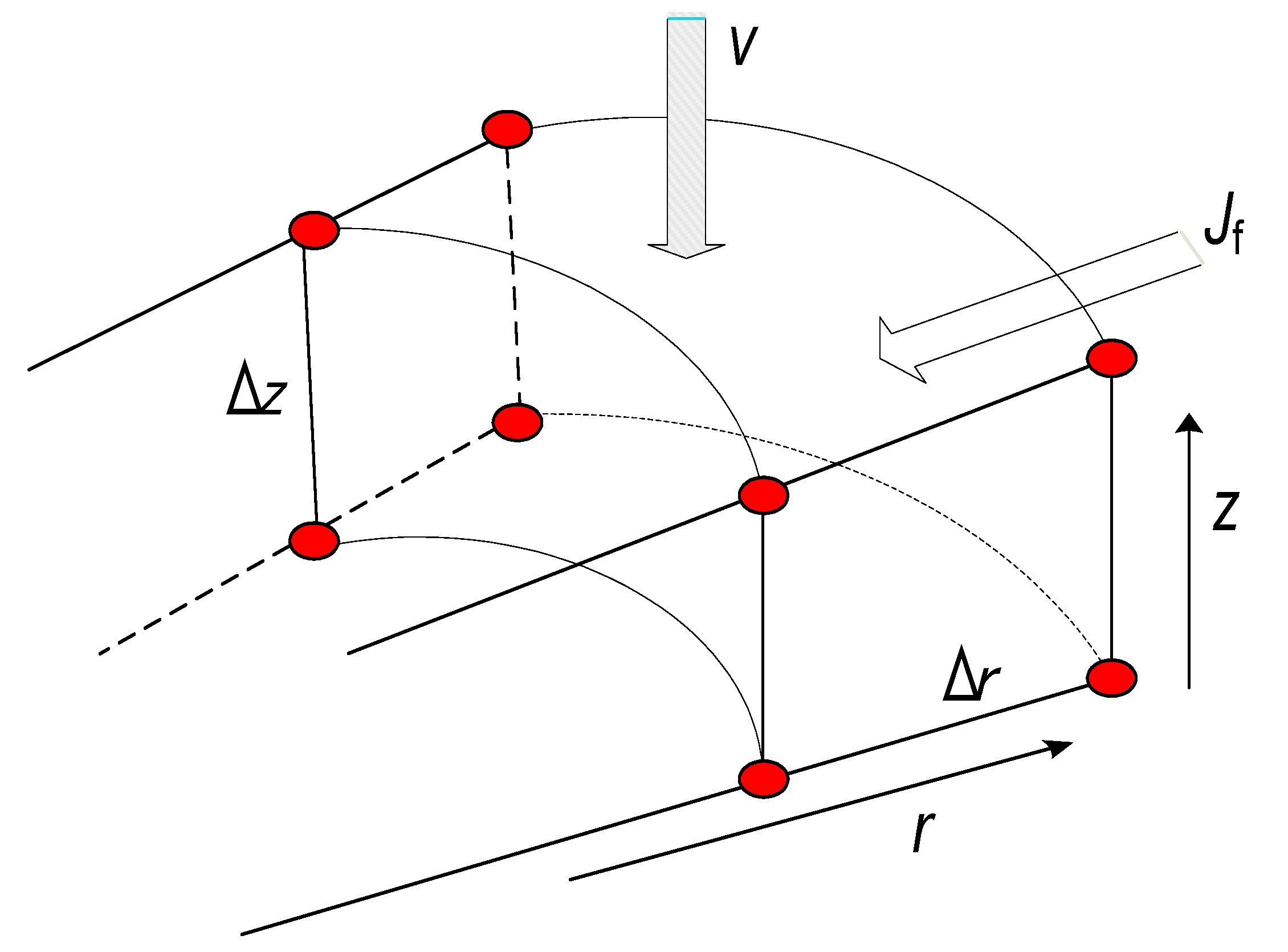
The unsteady state mass balance for solvent propane over a differential element of the medium (see Figure 2) is given by

(1)

where V = 2πr ΔrΔz is the volume of the element, A = 2πr Δr is the area transverse to the live oil velocity v in the vertical direction, and S = 2πr Δz is the area transverse to the dispersive flux J_f in the radial direction.

Figure 2. Differential element of the physical model.

Figure 2. Differential element of the physical model.

In Equation(1), the diffusive flux along the vertical direction is assumed insignificant in comparison with the convective flux.

Assuming constant live oil density; the radial flux can be written as

(2)

where D is the undetermined concentration-dependent dispersion coefficient of propane in the porous medium. Taking the limits of Δr and Δz to zero, the above equations yield the following mass transfer model:

(3)

where ω(t,r,z) is the mass fraction of solvent in bitumen, which is a function of time, radius and height of the porous medium. The velocity of the live oil along the vertical direction is the Darcy velocity given by

(4)

where K_t is relative permeability of the medium, K is its permeability, ρ is the density of live oil, g is gravity, and μ is the live oil viscosity.

Experimental live oil viscosity and propane solubility data were best fitted to obtain the live oil viscosity concentration-dependent model. The empirical correlation for the propane-heavy oil system during the process at the operating temperature and pressure is μ = μ₀ω⁻² with a high value of 0.982 for the r²-coefficient of determination.

The live oil drainage with time reduces the height of the bitumen, Z(t,r), in the packed medium. The change in the height with time at any radial location is given by

(5)

where v(t,r,0) is Darcy velocity at the bottom of the model at a given r.

Initially there is no gas inside the packing and no production of the live oil. The initial height of the bitumen sample is Z₀. The packing surface has the solvent gas concentration equal to its interface saturation concentration under prevailing temperature and pressure. Thus, the initial conditions at t = 0 are as follows:

(6)

At all times, the entire exposed circumference and the bottom face of the cylinder is saturated with gas. The solvent–heavy oil interface at the top moves down and the height of the bitumen, Z(r), decreases with time due to live oil drainage. Thus, we have a moving boundary problem which is described by Equation (5).

The heavy oil at the moving interface is saturated with gas at all times. Consequently, the boundary conditions are

ω[t,r,Z(t)] = ω(t,R,z) = ω(t,r,0) = ω_int

(7)

Because of symmetry

(8)

at all times.

3.2. The Mathematical Objective

It is desired to find the optimal dispersion function, D(ω), such that the difference between the model-calculated and experimental cumulative live oil produced is minimum. Mathematically, the objective functional can be written as

(9)

where I is the objective functional that needs to be minimized using the control function D = D[ω(t,r,z)]; m_e(t) is the experimental cumulative mass of the live oil produced at any time t, and m_c(t) is the model cumulative predicted mass of the live oil produced at any time t. The calculated mass m_c(t) is given by

(10)

Now, Equation (9) can be written as

(11)

subject to Equation (3), which in turn can be written as

(12)

where

(13)

and subject to Equation (5), which can be written as

(14)

where

f₂ = −v(t,r,0) = −α[ω(t,r,0)]²

(15)

Equation (12) and Equation (14) are the constraints for Equation (9), and D is the control function. Equation (12) and Equation (14) are highly non-linear partial differential equations. Therefore, two undetermined adjoint variables λ(t,r,z) and γ(t,r) are introduced into Equation (9) to yield the following unconstrained objective functional:

(16)

Substituting for G(t,r,z) and F(t,r) in the above equation yields

(17)

The minimization of J is now equivalent to the minimization of I. The variational derivative of J with respect to the optimization variable D will provide the conditions necessary for the minimum of J.

3.3. Determination of Necessary Conditions

In this section, we derive the necessary conditions for the minimum of J. Consider the variation of J as follows

(18)

where

(19)

(20)

(21)

Substitution of Equations (19), (20), and (21) into Equation (18) yields

(22)

Integration by parts of the second integral of the above equation yields

(23)

The first integral on the right hand side in Equation (23) is eliminated based on the nature of the process as follows: Because the solvent mass fraction is known at t = 0, its variation is ruled out, i.e.,

δ ω(0,r,z) = 0

(24)

The final mass fraction of solvent in bitumen is not specified. Thus, the variation due to the mass fraction is eliminated if its multiplicative term is forced to zero, i.e.

λ(T,r,z) = 0

(25)

Substitution of Equation (24) and Equation (25) into Equation (23) results in

(26)

Integration by parts of the fourth integral of Equation (22) yields

(27)

Since the solvent mass fraction in bitumen is specified for all r and t, the variation δ ω(t,r,Z) = 0 Hence

(28)

Integration by parts of the fifth integral of Equation (22) yields

(29)

Since the solvent mass fraction in bitumen, ω(t,R,z), is known for all z and t, the variation is zero. The mass fraction of solvent in bitumen, ω(t,0,z), is not specified. Variation due to ω(t,0,z) is eliminated if its multiplicative term is forced to zero, i.e.

λ(t,0,z) = 0

(30)

The above equation leads to

(31)

Integration by parts of the sixth integral of Equation (22) yields

(32)

Application of Equation (30) eliminates the second term on right hand side of Equation (32). To eliminate the first term on right hand side of Equation (32), the multiplicative term is forced to zero, i.e.

λ(t,R,z) = 0

(33)

The above conditions reduce Equation (32) to

(34)

Integration by parts of the eight integral of Equation (22) yields

(35)

The first integral on right hand side in Equation (35) is eliminated as follows. The initial height of bitumen, Z(0,r), is known, then the variation of Z(0,r) is ruled out, i.e.

δ Z(0,r) = 0

(36)

The final height of bitumen, Z(T,r), is not specified. Variation due to the final height is eliminated if its multiplicative term is forced to zero, i.e.

γ(T,r) = 0

(37)

Substitution of Equation (36) and Equation (37) in Equation (35) results in

(38)

The last integral of Equation (22) yields

(39)

Finally, substitution of Equations (26), (28), (31), (34), (38) and (39) into Equation (22) results in

(40)

At the minimum, δ J given by Equation (40) should be zero. That is only possible when the variational derivative of J with respect to D is

(41)

subject to the following adjoint equations:

(42)

(43)

(44)

Thus, Equation (41) is the necessary condition for the minimization of J when the continuity equation, as well as the adjoint equations [Equations (42)–(44)] are satisfied.

3.4. Adjoint Equations

Using Equations (13), (15), (42) and (44) we obtain

(45)

(46)

The boundary conditions for Equation (45) are

λ(T,r,z) = 0

(47)

λ(t,0,z) = λ(t,R,z) = 0

(48)

The boundary condition for Equation (43) is

γ(T,r) = 0

(49)

4. Computational Algorithm

Since Equations (12), (14), (43) and (45) are nonlinear partial differential equations, an analytical solution is not possible. Therefore, the problem is solved numerically. Based on the necessary conditions for the minimum of J, the following computational algorithm is applied to minimize J, and determine the concentration-dependent solvent dispersion function:

• Initialize dispersion function.
• Simultaneously integrate the continuity equation [Equation (12)] and Equation (14), subject to the initial and boundary conditions, to obtain the values of ω(t,r,z) and Z(t,r) for each node.
• Calculate the objective function given by Equation (9).
• Simultaneously integrate Equation (43) and Equation (45) backward, subject to the final boundary conditions, using stored values of ω and Z to get the values of λ(t,r,z) and γ(t,r) for each grid point.
• Improve D(ω) using the gradient correction given by Equation (41).
• Go to Step 2 until the improvement in J is negligible.

4.1. Implementation

The gradient correction for D(ω) was calculated as follows:

(50)

In addition, the gradient correction J_D was scaled to the magnitude of current dispersion values as follows:

(51)

where ε² is a small adjustable parameter, J_DS(k) is the scaled gradient correction at a specified gas mass fraction of the dispersion function, and n is the number of specified gas mass fractions of the dispersion function. Using the scaled gradient correction, the iterative improvement in the value of D(ω) was given by

D_i+1 = D_i − β_iJ_DS,i

(52)

where β_i is the optimal step length along the search direction in the ith iteration. The dispersion was considered to be discrete function, D(ω), at specified gas mass fractions between zero and the maximum concentration of the solvent in bitumen. D(ω) was initialized to a uniform value as high as possible without causing m_c(t) to intersect m_e(t). Equations (12), (14), (43), and (45) were finite-differenced along r and z directions. The resulting set of ordinary differential equations written for corresponding grid points are given in Appendix A. The details of the variational derivative of J with respect to D are provided in Appendix B.

With an accuracy of 10⁻⁶ in the time domain, the equations were numerically integrated using semi-implicit Bader-Deuflhard algorithm, and adaptive step size control [13]. Analytical Jacobian of Equations (12), (14), (43), and (45) was employed in the calculations. To fix the number of grid points along the r and z directions, N_t and N_z, the equations were integrated with increasing the number of grid points until the changes in the solution became negligible. The gradient correction in D(ω) was applied to the dispersion using Broyden-Fletcher-Goldfarb-Shanno algorithm [14,15].

Programmed in C++ language, the developed algorithm was implemented on Itanium 2/ Intel Itanium processor (1.5 GHz, 15.9 GB of RAM) with Intel C++ compiler. The algorithm took about 20 h to converge. During the computations, cubic splines were used to interpolate D(ω) as well as its first and second derivatives with respect to (ω); m_c(t) and m_e(t); ω(t) and Z(t); and the variational derivative J_D at each specified solvent mass fraction.

5. Results and Discussion

The above computational algorithm was applied to the experimental vapor extraction of heavy oil by propane. The experimental data of live oil production were used in the simulation of the developed model to determine the concentration-dependent dispersion function of propane in heavy oil. Table 2 lists the various parameters used in the simulation of the mathematical model.

Table 2. Model parameters.

Parameter	Value
φ	0.38
Kt	1
K, m2	2.013 × 10−10
R, m	0.03
Z0, m	0.25
μ0, kg/m·s	1.158 × 10−3
ρ, kg/m³	830

Table 2. Model parameters.

Parameter	Value
φ	0.38
Kt	1
K, m2	2.013 × 10−10
R, m	0.03
Z0, m	0.25
μ0, kg/m·s	1.158 × 10−3
ρ, kg/m³	830

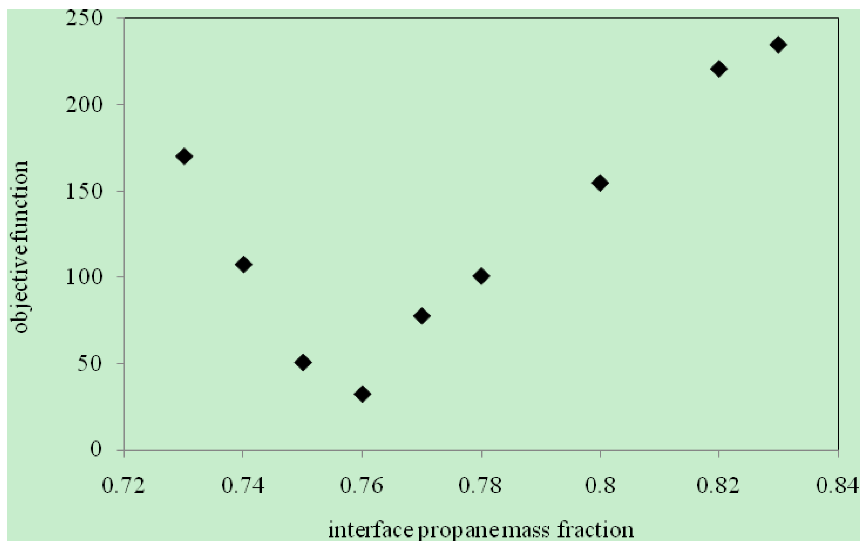
The objective function [Equation (9)] was obtained by solving Equations (A-1) to (A-26) with various values of ω_int in the range of 0.70–0.9 and the initial uniform dispersion function D(ω) in the range of 10⁻⁷ − 2.5 × 10⁻⁵ m²/s. In order to obtain the optimal value for propane mass fraction at the interface to solve equations, the minimum resultant objective functions were plotted against ω_int as shown in Figure 3. The optimal propane interface mass fraction ω_int was found to be 0.76. The above value of ω_int was used to determine the dispersion of propane as a function of its concentration in heavy oil. The results are presented in Figure 4, Figure 5 and Figure 6.

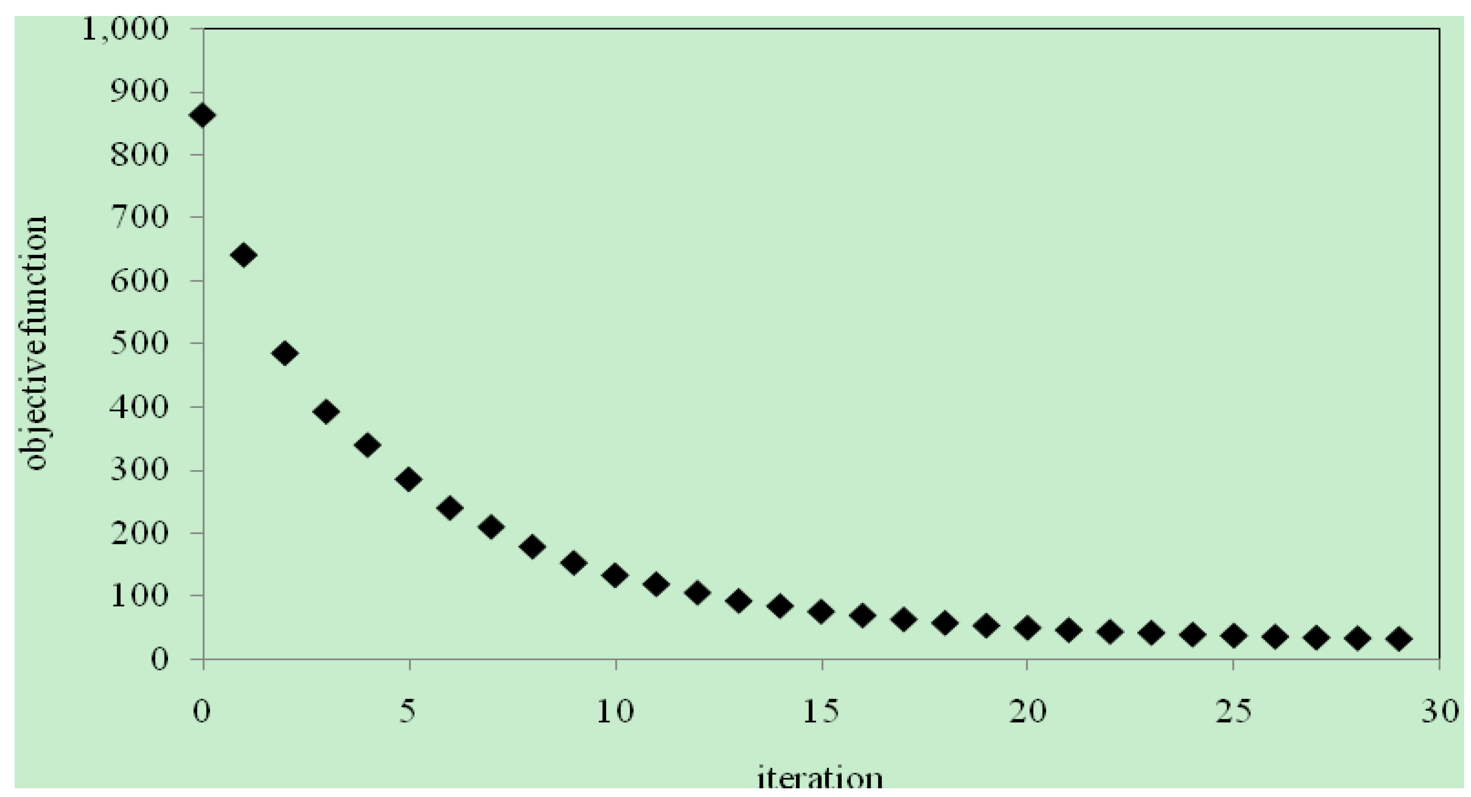
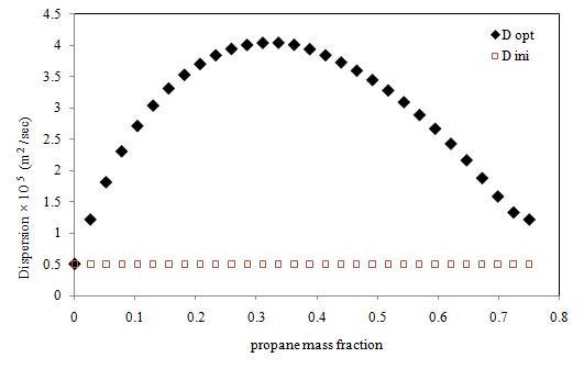
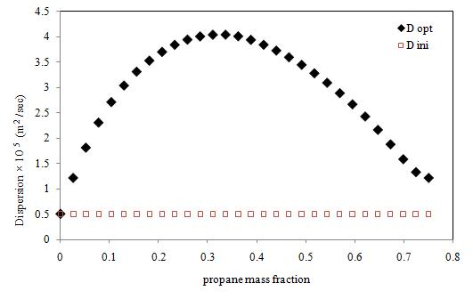
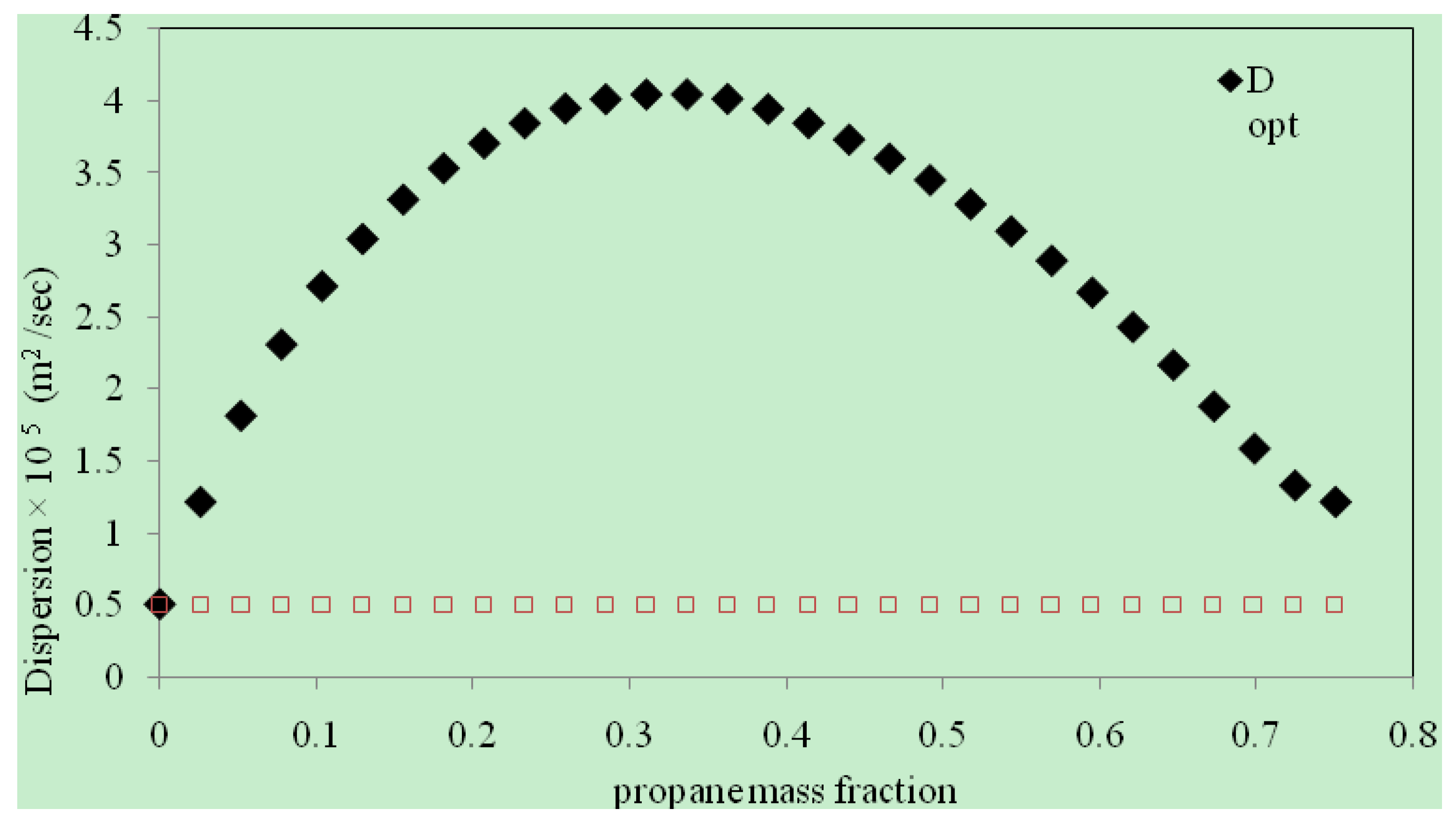
With ω_int = 0.76, the application of the algorithm resulted in an iterative reduction of the objective function accompanied by a corresponding improvement in D(ω). The objective function decreased monotonically to the minimum as shown in Figure 4. The final optimal function D(ω) was obtained in 29 iterations after which no further improvement was observed. The initial and final D(ω) are plotted Figure 5. It shows that the final, optimally determined D(ω) rises to a maximum value, and then drops toward the end. The maximum value of propane dispersion is 4.048 × 10⁻⁵ m²/s at the propane mass fraction of 0.336. This result is for the propane–heavy oil system at 21–22 °C and 0.689 MPa. 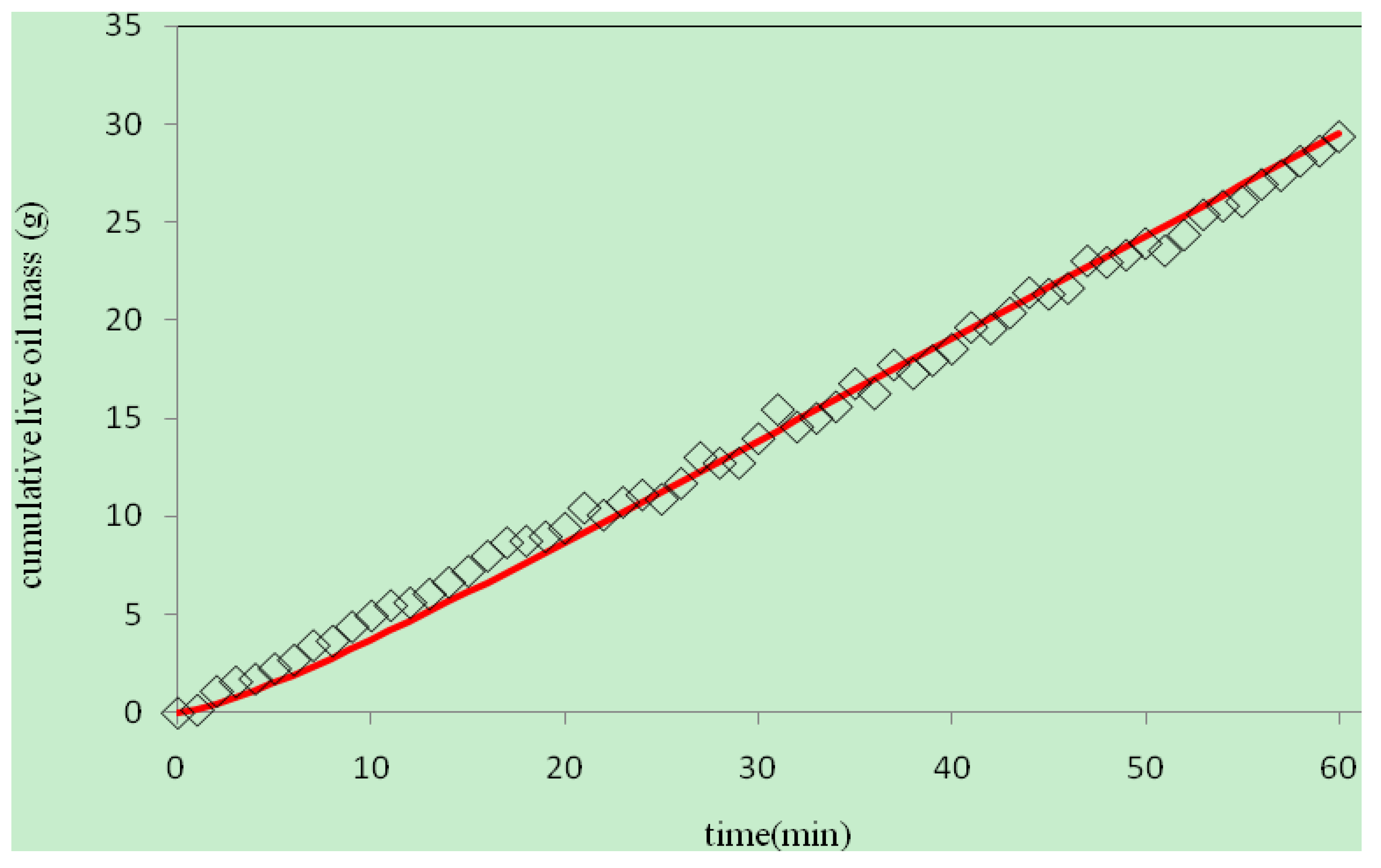Figure 6 compares the experimental live oil production to the calculated one with the optimally determined propane dispersion. It is observed that the experimental and calculated live oil productions agree very well. The calculated production follows experimental production very closely during the operation time of about 60 minutes.

Figure 3. Solvent interface mass fraction versus objective function.

Figure 3. Solvent interface mass fraction versus objective function.

The concentration dependence of dispersion coefficient is expected since the phenomenon of diffusivity embodied in dispersion is strongly affected by solvent concentration. The maximum in the concentration-dependent dispersion function could be explained as follows. Initially when higher concentration gradients are present in the heavy oil, the diffusion of solvent molecules is higher. It subsides later on with a gradual reduction in the concentration gradients as more and more solvent molecules penetrate the medium. When that happens, the diffusion of solvent molecules is restricted by their own abundance, thus decreasing the overall dispersion. Thus, at some intermediate stage, the diffusion coefficient is at its maximum. It has to be noted that we did not specify, or constrain the form of concentration-dependent dispersion function, but enabled its natural and realistic determination. In comparison to the molecular diffusion coefficient of propane in heavy oil [16,17,18], the average dispersion coefficient obtained in this work is up to four orders of magnitude higher, and underscores the strong effect of gravity-induced convection in Vapex.

Figure 4. Objective function versus iteration.

Figure 4. Objective function versus iteration.

Figure 5. Dispersion coefficient of propane in heavy oil at 21 °C and 0.689 MPa (diamond: the final, optimal dispersion coefficient, square: initial guess).

Figure 5. Dispersion coefficient of propane in heavy oil at 21 °C and 0.689 MPa (diamond: the final, optimal dispersion coefficient, square: initial guess).

The above outcome has a direct bearing on the optimal operations of Vapex implementations. For example, to maximize solvent uptake by the reservoir and oil production as a consequence, solvent injection rates should be such that the average solvent mass fraction in the reservoir (at 21–22 °C and 0.689 MPa) is close to the optimal solvent mass fraction (0.336) corresponding to the peak value of dispersion (4.048 × 10⁻⁵ m²/s; about twice the average value of dispersion). Hence, in addition to enabling more accurate reservoir simulations, the concentration-dependent dispersion function provide insights into optimizing Vapex operations as well.

Figure 6. Experimental and calculated mass of live oil produced with time (diamond: experimental mass, line: calculated mass).

Figure 6. Experimental and calculated mass of live oil produced with time (diamond: experimental mass, line: calculated mass).

6. Conclusions

A new technique was developed for the determination of concentration-dependent solvent dispersion in heavy oil. This technique was used to determine the dispersion coefficient of propane in heavy oil. The necessary conditions were derived for the match of the experimental cumulative oil produced with cumulative oil produced calculated from a Vapex mass transfer model. A computational algorithm was implemented to optimally compute dispersion coefficient as a function of the solvent mass fraction in heavy oil. The dispersion coefficient of propane in heavy oil was found to be a unimodal function of its mass fraction in heavy oil. The framework of optimal control, and the computational algorithm developed in this work could be applied to determine the concentration-dependent dispersion of other solvents used in the recovery of heavy oil and bitumen. Dispersion data will enable engineers to optimize oil production by operating Vapex close to the optimal solvent concentration corresponding to peak solvent dispersion.