Electrostatic Discharge Current Linear Approach and Circuit Design Method

 ,
,
Abstract
:1. Introduction
2. The Discharge Current of ESD
2.1. The Need for an Analytical and Accurate Equation for the ESD Current


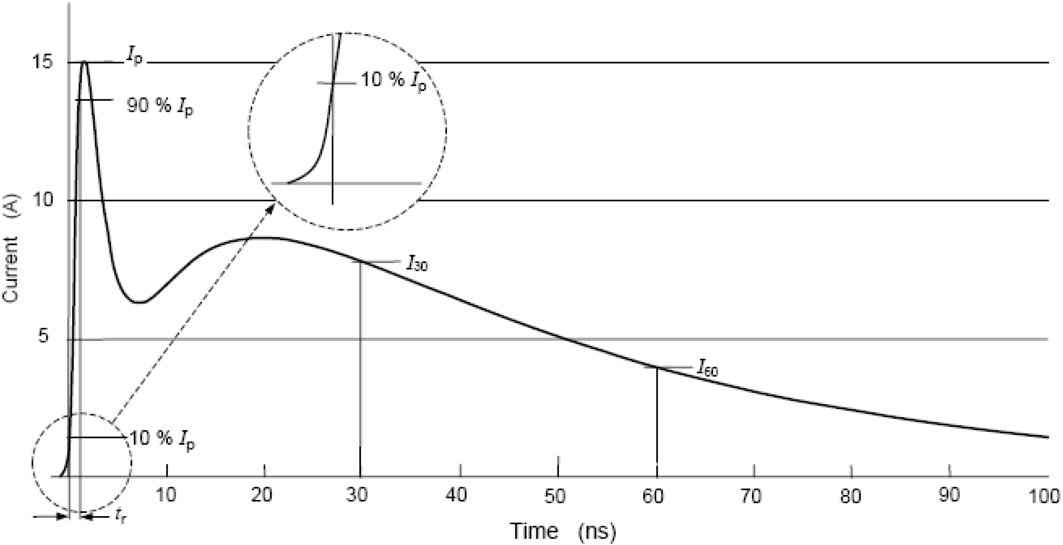
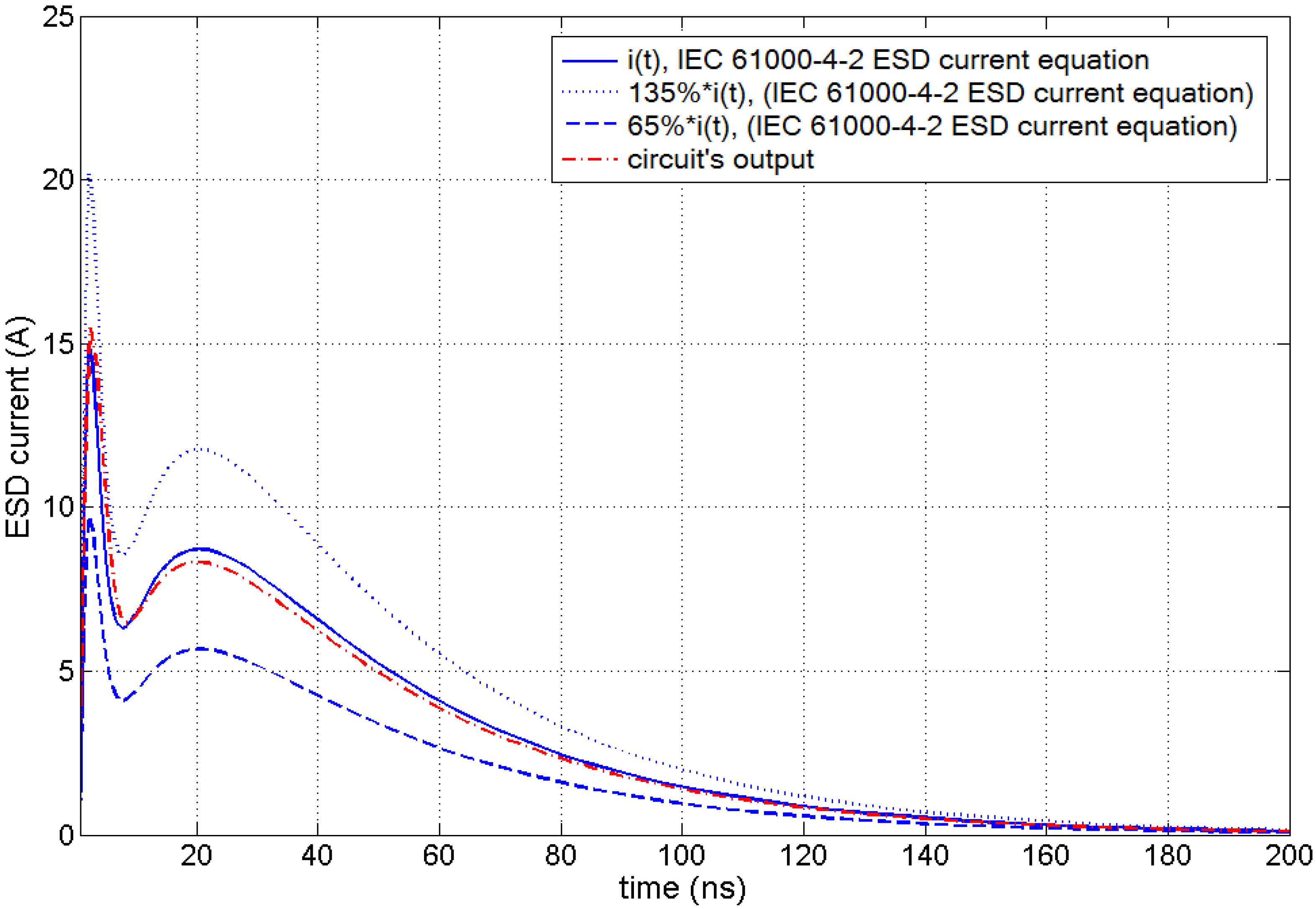
2.2. Equation of the ESD Current
- the first peak current (Ip);
- the rise time (tr), that is the time duration between the moment when the value of the ESD current is for the first time equal to 10% of its maximum value and the moment when the ESD current reaches for the first time 90% of its maximum value;
- the current at 30 ns (I30 ns), that is the value of the current 30 ns after the moment when the current has reached for the first time 10% of its maximum value, and
- the current at 60 ns (I60 ns), that is the value of the current 60 ns after the moment when the current has reached for the first time 10% of its maximum value.

| Parameter | Values of the Parameters of the ESD Current Defined by the IEC 61000-4-2 Standard | Values of the Parameters of the ESD Current Calculated Using the IEC 61000-4-2 Equation for the ESD Current |
|---|---|---|
| Ip (A) | 15 ± 15% | 15.14 |
| tr (ns) | 0.8 ± 25% | 0.88 |
| I30 ns (A) | 8 ± 30% | 7.83 |
| I60 ns (A) | 4 ± 30% | 3.98 |
3. The Approximation Methods
3.1. The Basic Idea
3.2. The Prony Method
3.3. The Modified Method
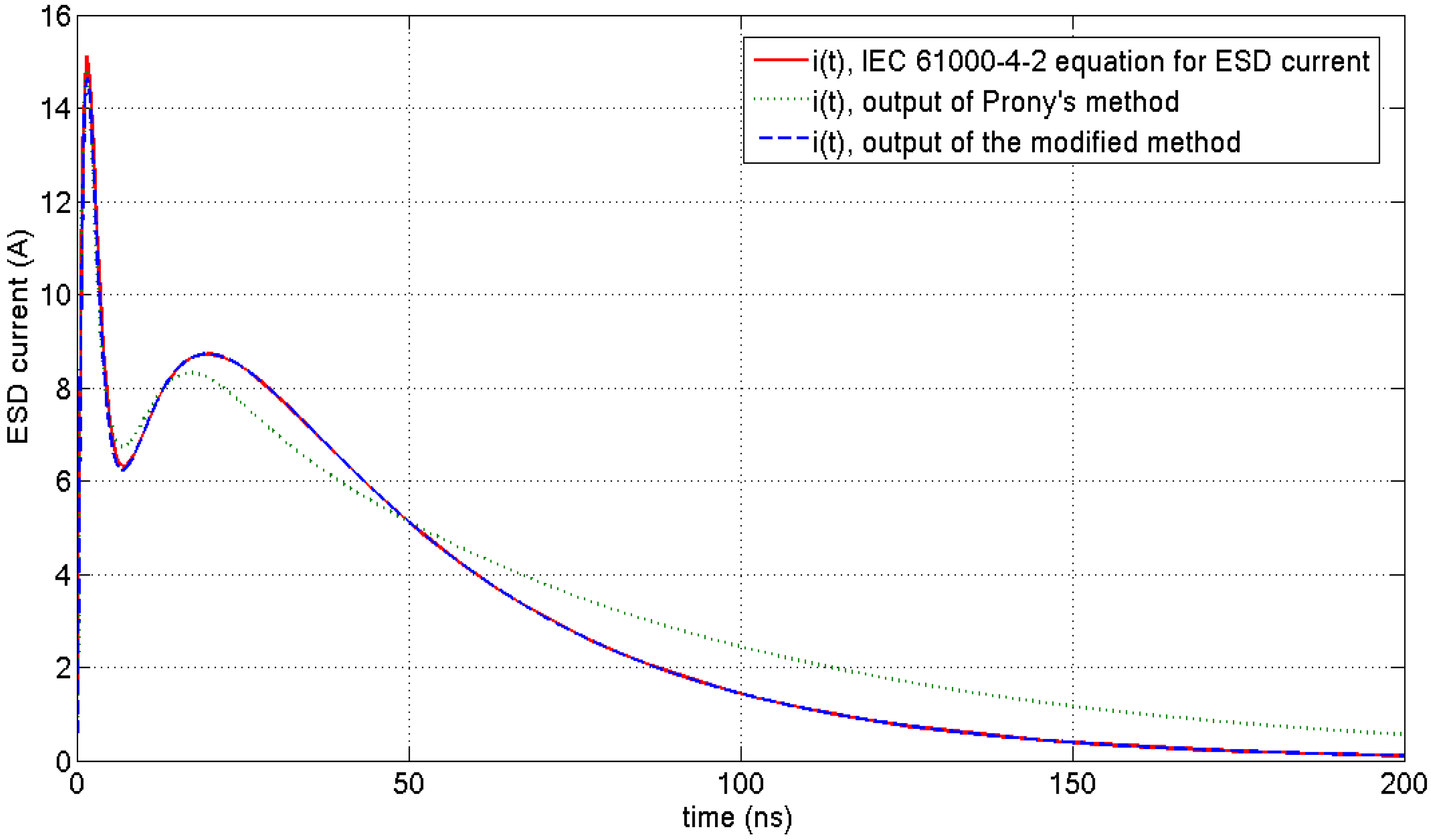
3.4. Applying the Approximation Methods
- Prony Method:
- Modified Method:
- Prony Method:
- Modified Method:
- Prony Method:
- Modified Method:

| Method | Time Interval | Relative Error Norm | |
|---|---|---|---|
| Maximum | Average | ||
| Prony Method | 2–60 ns | 50.43% | 5.69% |
| 0–200 ns | 50.43% | 21.23% | |
| Modified Method | 2–60 ns | 12.19% | 0.45% |
| 0–200 ns | 12.19% | 0.32% | |
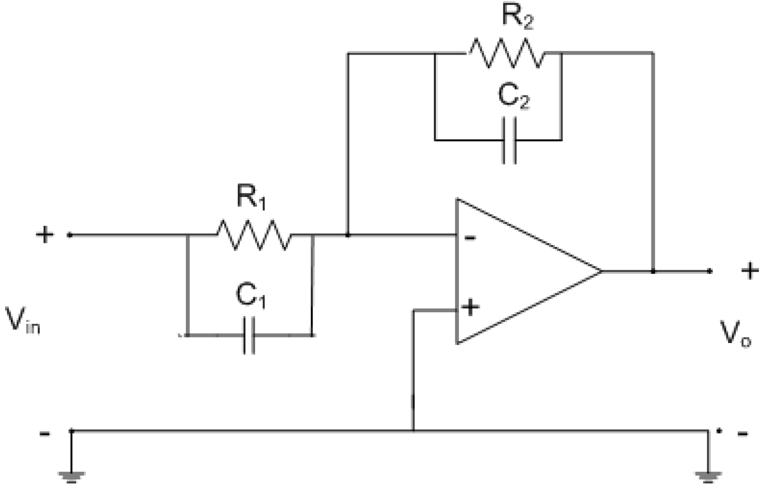
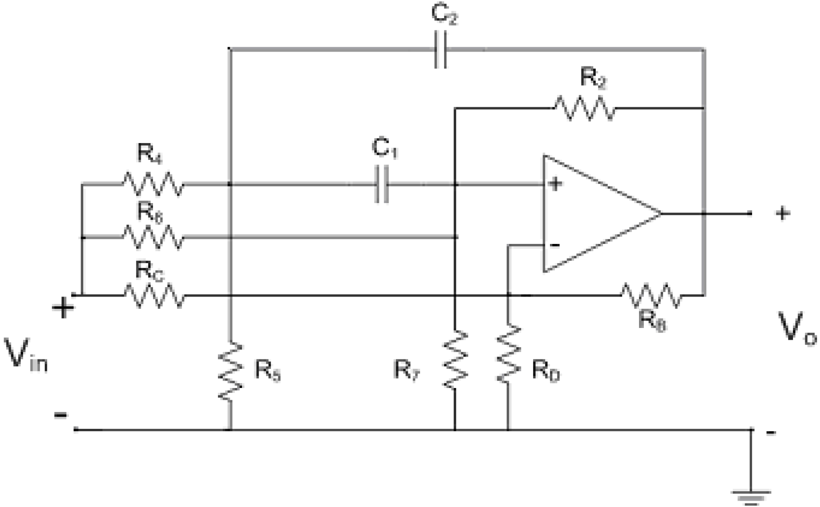
3.5. The Transfer Function
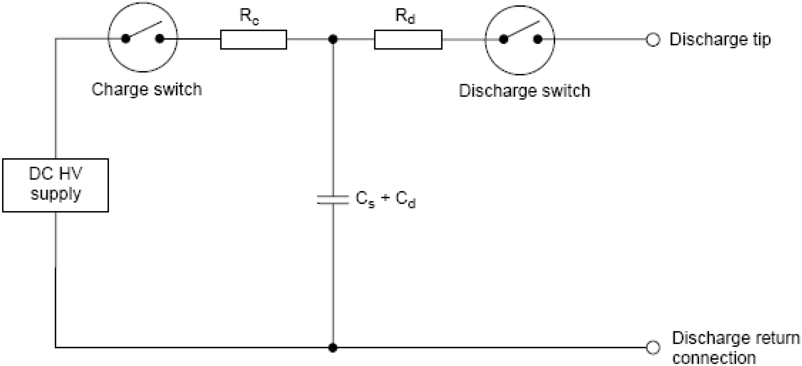
4. The Circuit


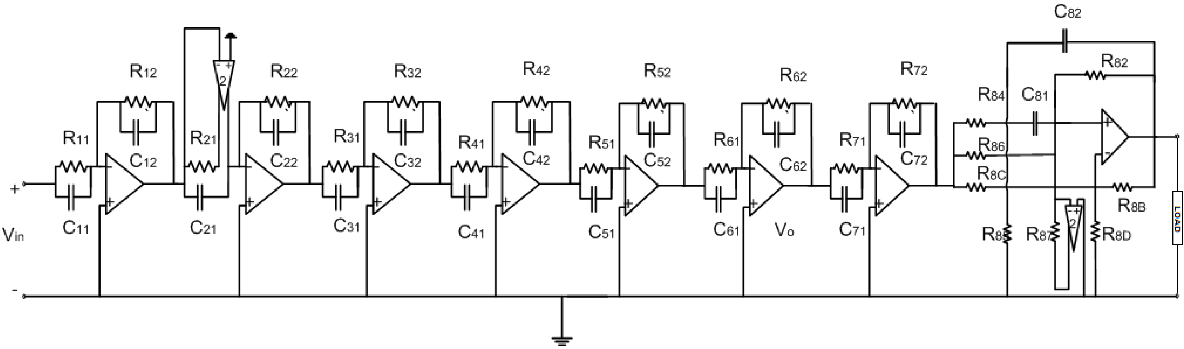
| I | Ri,1 (Ω) | Ri,2 (Ω) | Ci,1=Ci, (pF) |
|---|---|---|---|
| 1 | ∞ | 3.84 | 104 |
| 2 | 1.77 | 49.85 | 1 |
| 3 | 8.85 | 11.95 | 103 |
| 4 | 2.86 | 5.59 | 103 |
| 5 | 1.56 | 32.07 | 102 |
| 6 | 0.73 | 20.49 | 102 |
| 7 | 0.38 | 74.91 | 10 |
| R8,2 (Ω) | R8,4 (Ω) | R8,5 (Ω) | R8,6 (Ω) | C8,1 (nF) |
| 0.32 | 1.15 | 1.00 | 1.01 | 1.00 |
| R8,7 (Ω) | R8,B (Ω) | R8,C (Ω) | R8,D (Ω) | C8,2 (nF) |
| 0.46 | 1.00 | 1.00 | 0.00 | 1.00 |
5. Conclusions
References
- Barth, J. Measurements of real ESD threats that have been ignored too long. IEEE Instrum. Meas. Mag. 2005, 8, 61–63. [Google Scholar] [CrossRef]
- Fujiwara, O.; Taka, Y. Gap Breakdown field caused by air discharge through hand-held metal piece from charged human-body. In Proceedings of the 2006 4th Asia-Pacific Conference on Environmental Electromagnetics, Dalian, China, 1–4 August 2006; pp. 103–106.
- Lou, L.; Liou, J.J. An Improved Compact Model of Silicon-Controlled Rectifier (SCR) for Electrostatic Discharge (ESD) Applications. IEEE Trans. Electron Devices 2008, 55, 3517–3524. [Google Scholar] [CrossRef]
- Huang, J.; Liu, S.; Wang, X.; Zhou, F.; Wang, L.; Gao, Y. Intrinsic Characterization of Human Metal ESD: Current, Electromagnetic Field and Displacement Current. In Proceedings of the 2006 4th Asia-Pacific Conference on Environmental Electromagnetics, Dalian, China, 1–4 August, 2006; pp. 518–520.
- Yuan, Z.; Li, T.; He, J.; Chen, S.; Zeng, R. New Mathematical Descriptions of ESD Current Waveform Based on the Polynomial of Pulse Function. IEEE Trans. Electromagn. Compat. 2006, 48, 589–591. [Google Scholar] [CrossRef]
- International Electrotechnical Commission. International Standard IEC 61000-4-2: “Electromagnetic Compatibility (EMC), Part 4: Testing and Measurement Techniques, Section 2: Electrostatic Discharge Immunity Test–Basic EMC Publication”, 2008.
- Fotis, G.P.; Gonos, I.F.; Iracleous, D.P.; Stathopulos, I.A. Mathematical analysis and simulation for the electrostatic discharge (ESD) according to the EN 61000-4-2. In Proceedings of the 39th International Universities Power Engineering Conference, Bristol, UK, 6–8 September 2004; pp. 228–232.
- Wang, K.; Pommerenke, D.; Chundru, R.; Doren, T.V.; Drewniak, J.L.; Shashindranath, A. Numerical modeling of electrostatic discharge generators. IEEE Trans. Electromagn. Compat. 2003, 45, 258–270. [Google Scholar] [CrossRef]
- Amoruso, V.; Helali, M.; Lattarulo, F. An improved model of man for ESD applications. J. Electrostat. 2000, 49, 225–244. [Google Scholar] [CrossRef]
- Fujiwara, O.; Tanaka, H.; Yamanaka, Y. Equivalent circuit modeling of discharge current injected in contact with an ESD-gun. Electr. Eng. Jpn. 2004, 149, 8–14. [Google Scholar] [CrossRef]
- Caniggia, S.; Maradei, F. Circuital and numerical modeling of electrostatic discharge generators. In Proceedings of the 14th IAS Annual Meeting, IEEE Industry Applications Conference, Kowloon, Hong Kong, 8 August 2005; pp. 1119–1123.
- Fotis, G.P.; Gonos, I.F.; Stathopulos, I.A. Determination of the discharge current equation parameters of ESD using genetic algorithms. IEE-Electron. Lett. 2006, 42, 797–799. [Google Scholar] [CrossRef]
- Fotis, G.P.; Gonos, I.F.; Assimakopoulou, F.; Stathopulos, I.A. Applying genetic algorithms for the determination of the parameters of the electrostatic discharge current equation. Inst. Phys. Publishing Meas. Sci. Technol. 2006, 17, 2819–2827. [Google Scholar] [CrossRef]
- Carriere, R.; Moses, R.L. High Resolution Radar Target Modeling Using a Modified Prony Estimator. IEEE Trans. Antennas Propog. 1992, 40, 13–18. [Google Scholar] [CrossRef]
- Pierre, D.A.; Trudnowski, D.J.; Hauer, J.F. Identifying linear reduced-order models for systems with arbitraryinitial conditions using Prony signal analysis. IEEE Trans. Autom. Control 1992, 37, 831–835. [Google Scholar] [CrossRef]
- Qi, L.; Qian, L.; Cartes, D.; Woodruff, S. Initial results in Prony analysis for harmonic selective active filters. In Proceedings of IEEE Power Engineering Society General Meeting, Montreal, Canada, 18–22 June 2006; p. 6.
- Li, D.; Cao, Y.; Wang, G. Online identification of low-frequency oscillation in power system based on fuzzy filter and Prony algorithm. In Proceedings of International Conference on Power System Technology, Chongqing, China, 22–26 October 2006; pp. 1–5.
- Daryanani, G. Principles of Active Network Synthesis and Design; Wiley: New York, NY, USA, 1976. [Google Scholar]
© 2010 by the authors; licensee MDPI, Basel, Switzerland. This article is an open access article distributed under the terms and conditions of the Creative Commons Attribution license (http://creativecommons.org/licenses/by/3.0/).
Share and Cite
Katsivelis, P.K.; Fotis, G.P.; Gonos, I.F.; Koussiouris, T.G.; Stathopulos, I.A. Electrostatic Discharge Current Linear Approach and Circuit Design Method. Energies 2010, 3, 1728-1740. https://doi.org/10.3390/en3111728
Katsivelis PK, Fotis GP, Gonos IF, Koussiouris TG, Stathopulos IA. Electrostatic Discharge Current Linear Approach and Circuit Design Method. Energies. 2010; 3(11):1728-1740. https://doi.org/10.3390/en3111728
Chicago/Turabian StyleKatsivelis, Pavlos K., Georgios P. Fotis, Ioannis F. Gonos, Tryfon G. Koussiouris, and Ioannis A. Stathopulos. 2010. "Electrostatic Discharge Current Linear Approach and Circuit Design Method" Energies 3, no. 11: 1728-1740. https://doi.org/10.3390/en3111728