LES of a Meso Combustion Chamber with a Detailed Chemistry Model: Comparison between the Flamelet and EDC Models

Abstract

The goal of this paper is to contribute to the design of high-performance mesocombustors, a field currently under rapid development, in particular for propulsion, e.g., for UAVs, and micro/meso-electrical power generators. This study is focused on a cylindrical combustor of 29 cm³, fuelled by methane and air, which provides 2 kW of thermal power. The device was entirely designed and built at the Sapienza University of Rome and coupled with an ultra-micro turbine. Two 3D LES simulations with detailed chemistry are presented. They differ only for the combustion models, so that a model comparison can be carried out. The calculated maximum temperature inside the chamber, the gas exhaust temperature and the combustion efficiency are compared and discussed. The results, reported at two different physical times, show the effects of the different combustion models, which predict different temperature and species concentration maps, but similar values for the combustion efficiency. Thermal, chemical and kinematic maps show that the Eddy Dissipation Concept allows for a more accurate estimatation of the performance parameters for application to first-order design procedures.

1. Introduction

An investigation of the performance of a combustor for possible use in micro- and ultra-micro gas turbines for both stationary and propulsion applications is presented in this paper. The field of micro-meso thermo-electric/electronic devices is rapidly developing under the pressure of evermore stringent requirements posed by the increasing need for portable power generation. There are three main areas of interest for micro-meso-combustion: terrestrial and marine propulsion, UAV (“Unmanned Aerial Vehicles”) for tactical and meteorological recognissance, and portable electrical power generation.

In the current literature [1,2] a mesoscale combustion regime is defined as one in which the flame scale is of the same order of magnitude as the thickness of the flame preheating zone. This implies that one of the characteristic dimensions of the combustor is of the order of the quenching diameter (millimeters to centimeters): According to this definition, the device studied here belongs to the class of meso-combustion chambers. Meso-scale systems behave differently than macro-scale ones, since in the former both the Reynolds and Peclet numbers are low, and consequently viscous and diffusive effects become more important.

Low Reynolds implies low turbulent intensities or even laminar flow fields, so that the turbulent contribution to mixing processes is scarce or totally absent. At the same time, purely diffusive processes are too slow to be effective.

Therefore, in scaled-down conventional combustors the conversion of chemical- into thermal energy can be severely limited by the decreased residence time, and in the worst case it can be totally prevented. The size reduction implies also larger heat losses that bring about a decline in the overall combustion efficiency and a reduction of the reaction temperatures, which in turn narrows the stability limits of the combustor by increasing the kinetic reaction times. For the above reasons, a proper management and understanding of the thermo chemical issues connected to size reduction are mandatory in order to build operationally efficient meso-combustors.

Previous work in micro/meso-propulsion related to scaling laws issues [3,4,5,6] and focuses predominantly on fluid dynamics and combustion [7,8,9,10,11,12,13,14,15,16,17,18]. Three dimensional numerical simulations of methane-air combustion in swirling micro/meso-combustors are not common: the majority of the references available in the literature investigate the combustion process of propane in micro/meso sized combustor by assuming 2-D axi-symmetrical geometry and reduced kinetic mechanism [7,8,9,10,11,12,13,16,17,18].

Six of the above references deal with methane fuel, and while five of them [10,11,14,15,16,17,18] consider 2-D combustion chambers, only one of them analyzes 3-D swirling combustion chambers as in the present work; in [19] flame stabilization and flow evolution are analyzed mostly by means of experiments on swirling combustion chambers fueled by hydrogen, methane and propane. Microchambers are much smaller than the one presented here. Combustion efficiencies in excess of 90%, in particular with hydrogen, were reported; in combustion chambers smaller than 124 mm³, stable methane combustion could be achieved only by enriching air with oxygen. Results were compared with CFD simulations employing the global 1-step Westbrook and Dryer kinetic scheme [20]. Our work differs from that of [19] in two aspects: the chamber dimension and the accuracy of the chemical model.

In the following, two simulation campaigns on the same combustion chamber are reported. In the “Flamelet simulation”, combustion is modeled by means of 67 “flamelets” pre-calculated and stored in look-up tables [21,22,23,24,25,26,27,28] using detailed chemistry [29] (GRIMech3.0, 53 species and 325 reactions, using Arrhenius relations).

The “EDC simulation” employs the Eddy Dissipation Concept [30,31], and models chemistry with a detailed mechanism (GRIMech1.2) defined by 35 species and 177 reactions, using Arrhenius relations [32].

The EDC solves the species- and NS equations simultaneously. The GRIMech1.2 mechanism has been chosen to reproduce the chemistry as accurately as possible while abiding by the constraints posed by the CFD software (FLUENT6.3) [33] capabilities that limit the species equations to a maximum of 50.

Both simulations are performed by means of a 3D unsteady LES method with the “WALE” (Wall Adapting Local Eddy Viscosity) subgrid scale model [34], following the results provided in [35].

Temperature, species maps and combustion efficiency values are the most important results presented and discussed. The “Flamelet simulation” results are provided after 0.03 s of physical time while those of the “EDC simulation” are provided at two different times, namely after 0.03 s (3 residence times) and 0.05 s (five residence times).

The “EDC simulation” provides more realistic results than the first one, and it will be argued in the following that the differences result from the different assumptions posited by the two combustion models.

This paper is structured as follows: Section 2 describes the domain geometry and the specified operating conditions; Section 3 contains a brief discussion of the turbulence models; Section 4 discusses the combustion and chemistry models; Section 5 reports the numerical models while Section 6 presents and discusses the results.

This work is part of a broader work that includes an experimental analysis carried out at the Sapienza University of Roma, which will be reported and compared in a follow-up paper for a deeper understanding of combustion phenomena in microcombustion chambers.

2. Combustion Chamber and Operating Conditions

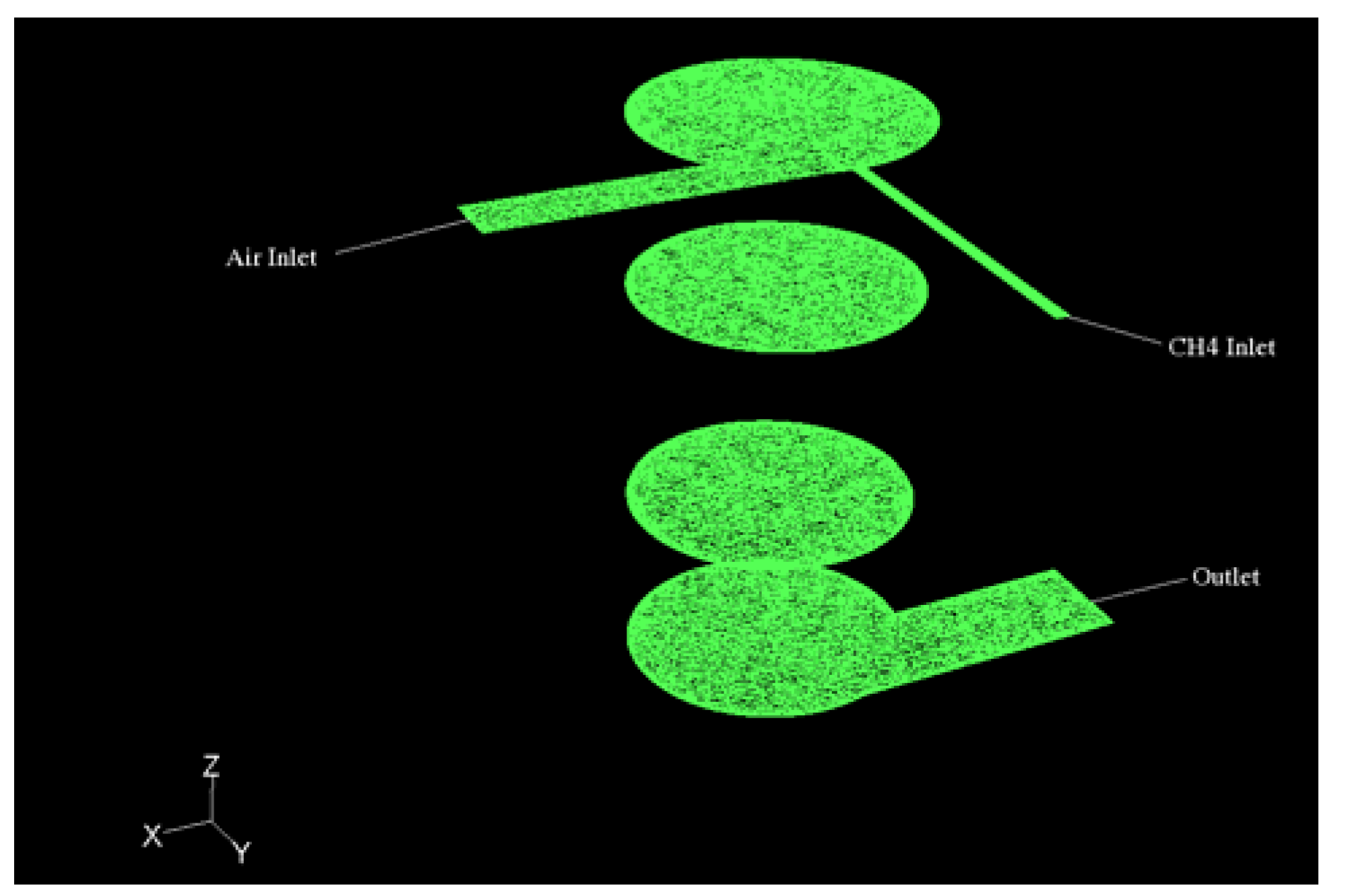
The combustion chamber geometry is reported in Figure 1 (divided into slices for ease of visualization): The domain is discretized by 870,000 unstructured cells, so that y⁺ ≈ 5 and Δy⁺ ≈ 1; that is, the first point away from the wall is inside the viscous sublayer, where the velocity profiles, in spite of the high stretching imposed by the elongated geometry, are still parabolic.

The diameter of the chamber is 0.025 m, its height 0.06 m (aspect ratio = 0.416), for a total volume of 29 cm³. The methane feeding duct has a diameter of 0.0015 m, the air duct 0.005 m. The exhaust duct on the lower side of the chamber has a diameter of 0.01 m.

To improve mixing the gaseous methane is injected in the radial direction at 90° with respect to the air flow which is tangential to the chamber. The dimensions of the chamber have a strong influence on the mixing dynamics, and consequently on the combustion efficiency, due to the strong effects of the aspect ratio (S/V) on the mean streamline curvature and on the swirling motions.

Operating and boundary conditions are reported in Table 1; mass flows at inlets are imposed, together with the pressure of 2 atm at the outlet section, while the walls are at constant temperature: Two different values were specified depending on the device zones: the chamber and air duct walls are at 700 K while the methane and exhaust ducts are at 300 K.

The fuel inlet Reynolds number is in the transitional regime (Re_CH4 = 1,500), while the Re_air is fully turbulent (Re_AIR = 14,700); this feature is characteristic (and peculiar) of microcombustors; it is well known that the possibility of relaminarization is enhanced by combustion that causes an increase of the effective viscosity of the burning mixture; on the other hand, the slight expansion inside of the chamber introduces a contrasting effect, so that the final regime is determined by the dynamic competition between these two effects.

Figure 1. Representative geometry of the micro-combustion chamber.

Figure 1. Representative geometry of the micro-combustion chamber.

Table 1. Operating Conditions.

Parameter	Methane	Air
Mass Flow Rate (kg/s)	3.93 × 10−5	1.9 × 10−3
Inlet Temperature (K)	300	700
Outlet Pressure (atm)	2	2
Inlet Velocity (m/s)	18	100
Inlet Viscosity (kg/m-s)	2 × 10−5	3.29 × 10−5
Re	1,500	14,700
Chamber Wall Temperature (K)	700
Methane Duct Wall Temperature (K)	300
Air Duct Wall Temperature (K)	700
Exhaust Duct Wall Temperature (K)	300
Kinetic Energy Ratio, M	0.038
Global equivalence ratio	0.355

Table 1. Operating Conditions.

Parameter	Methane	Air
Mass Flow Rate (kg/s)	3.93 × 10−5	1.9 × 10−3
Inlet Temperature (K)	300	700
Outlet Pressure (atm)	2	2
Inlet Velocity (m/s)	18	100
Inlet Viscosity (kg/m-s)	2 × 10−5	3.29 × 10−5
Re	1,500	14,700
Chamber Wall Temperature (K)	700
Methane Duct Wall Temperature (K)	300
Air Duct Wall Temperature (K)	700
Exhaust Duct Wall Temperature (K)	300
Kinetic Energy Ratio, M	0.038
Global equivalence ratio	0.355

The species isobaric specific heats are described by polynomials in T as per the GRIMech Thermo Data file [36] that has been included in the CFD code, while kinetic theory [37] is assumed to predict transport properties.

3. Turbulence and Combustion Models

The LES modeling approach is applied in both simulations. They adopt the WALE (Wall Adapting Local Eddy viscosity) model [34] which is designed to return the correct y³ wall asymptotic behavior for wall bounded flows. As previously stated, the “flamelet simulation” uses the “non-adiabatic flamelet model” and the second the EDC model.

The flamelet model, used in the non-premixed combustion model to account for chemical non-equilibrium, regards the turbulent flame as an ensemble of thin, laminar, locally one-dimensional flamelet structures embedded within the turbulent flow field [21,22,24,25,26]. Here 67 flamelets, with χ₀ = 1 and Δχ = 2, have been used to describe combustion, where $\chi =2D{\left|\nabla f\right|}^2$ is the scalar dissipation [s⁻¹], D is the diffusion coefficient and f is the mixture fraction. N equations are solved for the species mass fractions, Y_i:

$$\rho \frac{\partial Y_i}{\partial t}=\frac{1}{2}\rho \chi \frac{{\partial }^2{Y}_i}{\partial f^2}+S_i$$

(1)

while the energy equation is solved for the temperature:

$$\rho \frac{\partial T}{\partial t}=\frac{1}{2}\rho \chi \frac{{\partial }^{2}T}{\partial f^2}-\frac{1}{c_p}{\displaystyle \sum _i{H}_i{S}_i+}\frac{1}{2c_p}\rho \chi \left[\frac{\partial c_p}{\partial f}+{\displaystyle \sum _i{c}_{pi}}\frac{\partial Y}{\partial f}\right]\frac{\partial T}{\partial f}$$

(2)

Equations 1 and 2 are solved separately and previously than the NS equations and stored in look-up tables as function of f and χ only. This means that the initialization field is the one at equilibrium in every cell, hence reaction rates do not respect the real thermodynamic conditions inside the chamber.

Reactions are described by the GRIMech3.0 [29] chemical mechanism (53 species and 325 reactions). The “EDC simulation” adopts the Eddy Dissipation Concept [31]. It assumes that reactions occur in small turbulent structures, called the fine structures [30], under a steady state assumption, according to the law:

$$R_i=\frac{\rho {\left(\xi *\right)}^2}{\tau *\left[1-{\left(\xi *\right)}^3\right]}\left(Y_i^{*}-Y_i\right)$$

(3)

where Y_i^* is the fine-scale species mass fraction after reacting over the time $\tau *=C_{\tau }{\left(\frac{\nu }{\epsilon }\right)}^{\frac{1}{2}}$.

Chemistry is defined by the GRIMech1.2 [32] chemical mechanism (35 species and 177 reactions).

Even though the two chemistry models differ both for the number of species they consider and for the number of reactions they include in the calculations, the results presented in this work can be under the specified assumptions- directly compared, for the following reasons:

(a)

The flamelet model is an equilibrium model, and as such it provides the solution at a hypothetical (locally steady) equilibrium: ignition delay is explicitly neglected, and therefore the only global quantity of interest is the final combustion temperature;

(b)

GRIMech1.2 and GRIMech3 predict in fact slightly different ignition delays, but this is unessential in this study, in which the comparison is made at the final equilibrium conditions. To witness, Table 2 reports the difference in the adiabatic flame temperature for several equivalence ratios and ignition temperatures: it is apparent that, in the range of interest here (see the temperature maps in Figures 8–10), the deviations are less than 0.5%.

Table 2. Final Temperature % difference between GRIMech3.0 and GRIMech1.2.

Reactants Temperature (K)	Φ = 0.3	Φ = 0.5	Φ = 0.7	Φ = 0.9	Φ = 1	Φ = 1.1	Φ = 1.3	Φ = 1.5	Φ = 1.7	Φ = 1.9	Φ = 1.1
1000	0.00%	−0.6%	–0.6%	–0.4%	–1.4%	–0.4%	–0.3%	4.2%	–0.04%	0.00%	–0.4%
1100	0.00%	–0.7%	–0.6%	–0.5%	–1.3%	–0.5%	–0.3%	3.5%	–0.04%	0.00%	–0.5%
1200	0.00%	–0.7%	–0.6%	–0.5%	–1.3%	–0.5%	–0.4%	2.8%	–0.04%	–0.04%	–0.5%
1300	–0.1%	–0.8%	–0.6%	–0.5%	–1.2%	–0.5%	–0.4%	–0.2%	–0.1%	–0.04%	–0.5%
1400	–0.1%	–0.9%	–0.6%	–0.5%	–1.2%	–0.5%	–0.4%	–0.3%	–0.1%	–0.04%	–0.5%
1500	–0.1%	–0.8%	–0.6%	–0.5%	–1.1%	–0.5%	–0.4%	–0.3%	–0.2%	–0.04%	–0.5%
1600	–0.1%	–0.8%	–0.5%	–0.5%	–1.1%	–0.5%	–0.4%	–0.3%	–0.1%	–0.1%	–0.5%
1700	–0.1%	–0.7%	–0.5%	–0.5%	–1.0%	–0.5%	–0.4%	–0.3%	–0.1%	–0.1%	–0.5%
1800	–0.3%	–0.7%	–0.5%	–0.5%	–1%	–0.5%	–0.5%	–0.3%	–0.2%	–0.1%	–0.5%
1900	–0.2%	–0.6%	–0.4%	–0.5%	–0.9%	–0.5%	–0.5%	–0.3%	–0.2%	–0.1%	–0.5%
2000	–0.2%	–0.5%	–0.6%	–0.5%	–0.9%	–0.5%	–0.5%	–0.4%	–0.3%	–0.1%	–0.5%

Table 2. Final Temperature % difference between GRIMech3.0 and GRIMech1.2.

Reactants Temperature (K)	Φ = 0.3	Φ = 0.5	Φ = 0.7	Φ = 0.9	Φ = 1	Φ = 1.1	Φ = 1.3	Φ = 1.5	Φ = 1.7	Φ = 1.9	Φ = 1.1
1000	0.00%	−0.6%	–0.6%	–0.4%	–1.4%	–0.4%	–0.3%	4.2%	–0.04%	0.00%	–0.4%
1100	0.00%	–0.7%	–0.6%	–0.5%	–1.3%	–0.5%	–0.3%	3.5%	–0.04%	0.00%	–0.5%
1200	0.00%	–0.7%	–0.6%	–0.5%	–1.3%	–0.5%	–0.4%	2.8%	–0.04%	–0.04%	–0.5%
1300	–0.1%	–0.8%	–0.6%	–0.5%	–1.2%	–0.5%	–0.4%	–0.2%	–0.1%	–0.04%	–0.5%
1400	–0.1%	–0.9%	–0.6%	–0.5%	–1.2%	–0.5%	–0.4%	–0.3%	–0.1%	–0.04%	–0.5%
1500	–0.1%	–0.8%	–0.6%	–0.5%	–1.1%	–0.5%	–0.4%	–0.3%	–0.2%	–0.04%	–0.5%
1600	–0.1%	–0.8%	–0.5%	–0.5%	–1.1%	–0.5%	–0.4%	–0.3%	–0.1%	–0.1%	–0.5%
1700	–0.1%	–0.7%	–0.5%	–0.5%	–1.0%	–0.5%	–0.4%	–0.3%	–0.1%	–0.1%	–0.5%
1800	–0.3%	–0.7%	–0.5%	–0.5%	–1%	–0.5%	–0.5%	–0.3%	–0.2%	–0.1%	–0.5%
1900	–0.2%	–0.6%	–0.4%	–0.5%	–0.9%	–0.5%	–0.5%	–0.3%	–0.2%	–0.1%	–0.5%
2000	–0.2%	–0.5%	–0.6%	–0.5%	–0.9%	–0.5%	–0.5%	–0.4%	–0.3%	–0.1%	–0.5%

4. Numerical Models

Simulations have been carried out with a Pressure-Based solver which employs an algorithm of the general class of “projection methods” [38]. In this method the constraint of mass conservation (continuity) of the velocity field is imposed by solving a pressure correction equation. This solver (Fluent 6.3) uses a solution algorithm where the governing equations are solved sequentially (segregated from one another).

The SIMPLEC (SIMPLE-Consistent algorithm) [39], with a skewness correction (particularly useful with this high curvature geometry) is used to resolve the pressure-velocity correcting equation; the SIMPLEC uses a relationship between velocity and pressure corrections to enforce mass conservation and to obtain the pressure field.

The unsteady formulation is discretized by a central 2nd order implicit scheme. The momentum equation, the energy and mixture fraction equations are discretized by the 3rd order MUSCL (Monotone Upstream-Centered Schemes for Conservatives Laws) scheme [40]: This scheme is derived by blending a central differencing scheme and a 2nd order upwind scheme. The pressure equation is discretized by a 2nd order method.

5. Results and Discussion

In the following a comparison between the two simulations is provided. For the sake of clarity all figures show the flowfields on slices located at 0.01 m, 0.03 m and 0.055 m, (the first and last being the inlet- and outlet plane respectively) and they are provided, wherever possible, using the same scale.

The results shown here correspond to two different physical times, namely 0.03 s and 0.05 s (three and five residence times, respectively).

The mean residence time can be defined as the time a parcel of gas spends inside the combustor, its value estimated as the ratio between the mass of gas in the chamber volume, $V_c\overline{\rho }$, and the mass flow rate, $\dot{m}$:

$${\tau }_{\text{residence}}=\frac{V_c\overline{\rho }}{\dot{m}}\approx 0.01\text{ s}$$

(4)

The total mass flow rate was computed from the data in Table 1, while the averaged gas density, $\overline{\rho }$, is assumed equal to that of air at 1,100 K and 2 bar (0.62 kg/m³). Assuming this residence time as the characteristic combustion chamber fluid dynamics time, and comparing it with data in Table 3 and Table 4, it is possible to deduce a “worst case Damkoehler number”.

The Damkoehler number, Da, defines the fluid-dynamics/chemical times ratio and indicates whether the reactions are completed within a given time (Da >> 1), or are frozen (Da << 1).

Table 3 and Table 4 report the ignition delay times, t_id, predicted at the combustion chamber pressure by the detailed GRIMech 3.0 mechanism [32] run for different values of the equivalence ratio Φ and for a temperature range from 1,000 K to 2,300 K (1,000 K being just above the auto ignition temperature and 2,300 K is the maximum temperature inside the chamber, for both simulations, at steady state).

In the worst case, to obtain Da >> 1 (complete reactions), combustion temperatures must be ≥1,300 K with Φ ~ 0.9. Figure 6 shows that wide zones of the chamber are well above 2,000 K.

The iterative solution was assumed converged when the difference between inlet and outlet mass flowrate, ∆m/∆t, was <1 × 10⁻⁷ kg/s (two and three orders of magnitude smaller than the methane and air mass flow rates, respectively). The integration time step was 1 × 10⁻⁷s, that is, 2 orders of magnitude smaller than the shortest ignition time (1 × 10⁻⁵ s) occurring for T = 2300 K and Φ ~ 1, see Table 3 and Table 4.

Table 3. Ignition Delay, s, 0.3 ≤ Φ ≤ 1.0.

Ignition Temperature (K)	Φ = 0.3	Φ = 0.5	Φ = 0.7	Φ = 0.9	Φ = 1
1000	0.608	0.772	0.982	1.03	1.03
1100	0.111	0.143	0.131	0.192	0.202
1200	0.0244	0.0314	0.0331	0.0424	0.044
1300	0.00649	0.00815	0.000967	0.011	0.0114
1400	0.00211	0.00247	0.00289	0.00323	0.00336
1500	0.000881	0.000915	0.00103	0.00112	0.00114
1600	0.000422	0.000398	0.000423	0.000439	0.000456
1700	0.000246	0.000197	0.000203	0.000203	0.000211
1800	0.000174	0.000108	0.000106	0.000107	0.000109
1900	0.000148	0.000067	0.0000638	0.0000627	0.0000628
2000	0.000139	0.0000398	0.0000381	0.0000375	0.0000377
2100	0.00017	0.0000263	0.0000247	0.0000241	0.000024
2200	0.000233	0.0000183	0.0000167	0.0000162	0.0000161
2300	-	0.0000156	0.0000118	0.0000114	0.0000113

Table 3. Ignition Delay, s, 0.3 ≤ Φ ≤ 1.0.

Ignition Temperature (K)	Φ = 0.3	Φ = 0.5	Φ = 0.7	Φ = 0.9	Φ = 1
1000	0.608	0.772	0.982	1.03	1.03
1100	0.111	0.143	0.131	0.192	0.202
1200	0.0244	0.0314	0.0331	0.0424	0.044
1300	0.00649	0.00815	0.000967	0.011	0.0114
1400	0.00211	0.00247	0.00289	0.00323	0.00336
1500	0.000881	0.000915	0.00103	0.00112	0.00114
1600	0.000422	0.000398	0.000423	0.000439	0.000456
1700	0.000246	0.000197	0.000203	0.000203	0.000211
1800	0.000174	0.000108	0.000106	0.000107	0.000109
1900	0.000148	0.000067	0.0000638	0.0000627	0.0000628
2000	0.000139	0.0000398	0.0000381	0.0000375	0.0000377
2100	0.00017	0.0000263	0.0000247	0.0000241	0.000024
2200	0.000233	0.0000183	0.0000167	0.0000162	0.0000161
2300	-	0.0000156	0.0000118	0.0000114	0.0000113

Table 4. Ignition Delay, s, 1.1 ≤ Φ ≤ 1.9.

Ignition Temperature (K)	Φ = 1.1	Φ = 1.3	Φ = 1.5	Φ = 1.7	Φ = 1.9
1000	1.15	1.26	1.22	1.43	1.53
1100	0.216	0.237	0.232	0.234	0.292
1200	0.0473	0.0522	0.0524	0.0323	0.0643
1300	0.0122	0.0134	0.0142	0.0155	0.0163
1400	0.00355	0.0039	0.00425	0.00445	0.00433
1500	0.00121	0.00127	0.00133	0.00143	0.00152
1600	0.00044	0.000492	0.000525	0.000529	0.000533
1700	0.000213	0.000221	0.00023	0.000236	0.000244
1800	0.000111	0.000112	0.000112	0.000116	0.00012
1900	0.0000623	0.0000623	0.0000623	0.0000627	0.0000638
2000	0.0000374	0.0000376	0.0000384	0.0000385	0.0000392
2100	0.0000239	0.000024	0.0000241	0.0000245	0.000025
2200	0.0000161	0.0000161	0.0000162	0.0000164	0.0000168
2300	0.0000112	0.0000112	0.0000113	0.0000115	0.0000118

Table 4. Ignition Delay, s, 1.1 ≤ Φ ≤ 1.9.

Ignition Temperature (K)	Φ = 1.1	Φ = 1.3	Φ = 1.5	Φ = 1.7	Φ = 1.9
1000	1.15	1.26	1.22	1.43	1.53
1100	0.216	0.237	0.232	0.234	0.292
1200	0.0473	0.0522	0.0524	0.0323	0.0643
1300	0.0122	0.0134	0.0142	0.0155	0.0163
1400	0.00355	0.0039	0.00425	0.00445	0.00433
1500	0.00121	0.00127	0.00133	0.00143	0.00152
1600	0.00044	0.000492	0.000525	0.000529	0.000533
1700	0.000213	0.000221	0.00023	0.000236	0.000244
1800	0.000111	0.000112	0.000112	0.000116	0.00012
1900	0.0000623	0.0000623	0.0000623	0.0000627	0.0000638
2000	0.0000374	0.0000376	0.0000384	0.0000385	0.0000392
2100	0.0000239	0.000024	0.0000241	0.0000245	0.000025
2200	0.0000161	0.0000161	0.0000162	0.0000164	0.0000168
2300	0.0000112	0.0000112	0.0000113	0.0000115	0.0000118

Flamelet results are provided at 0.03 s while EDC’s results at both 0.03 s and 0.05 s: This has been done to highlight the main characteristics of the two models.

The EDC model reproduces “in-evolution chemistry phenomena” while the flamelet model reaches a steady configuration much faster. This is due to the two different assumptions by the combustion models.

The flamelet model does not need to simulate the spark (the first ignition): flamelet calculations are function only of mixture ratio and scalar dissipation and then the initial solution is the equilibrium condition in every cell.

The EDC, on the contrary, needs to simulate the spark because it assumes an ignition temperature equal to the local cell temperature, so respecting reaction times as defined by the Arrhenius law. The “numerical spark” consisted of few cells close to the impingement region at temperature of 2,000 K.

Moreover, the EDC model explicitly accounts for species transport properties while the Flamelet assumes an overall transport property, in this case equal to that of the nitrogen that is the species with the highest mass fraction.

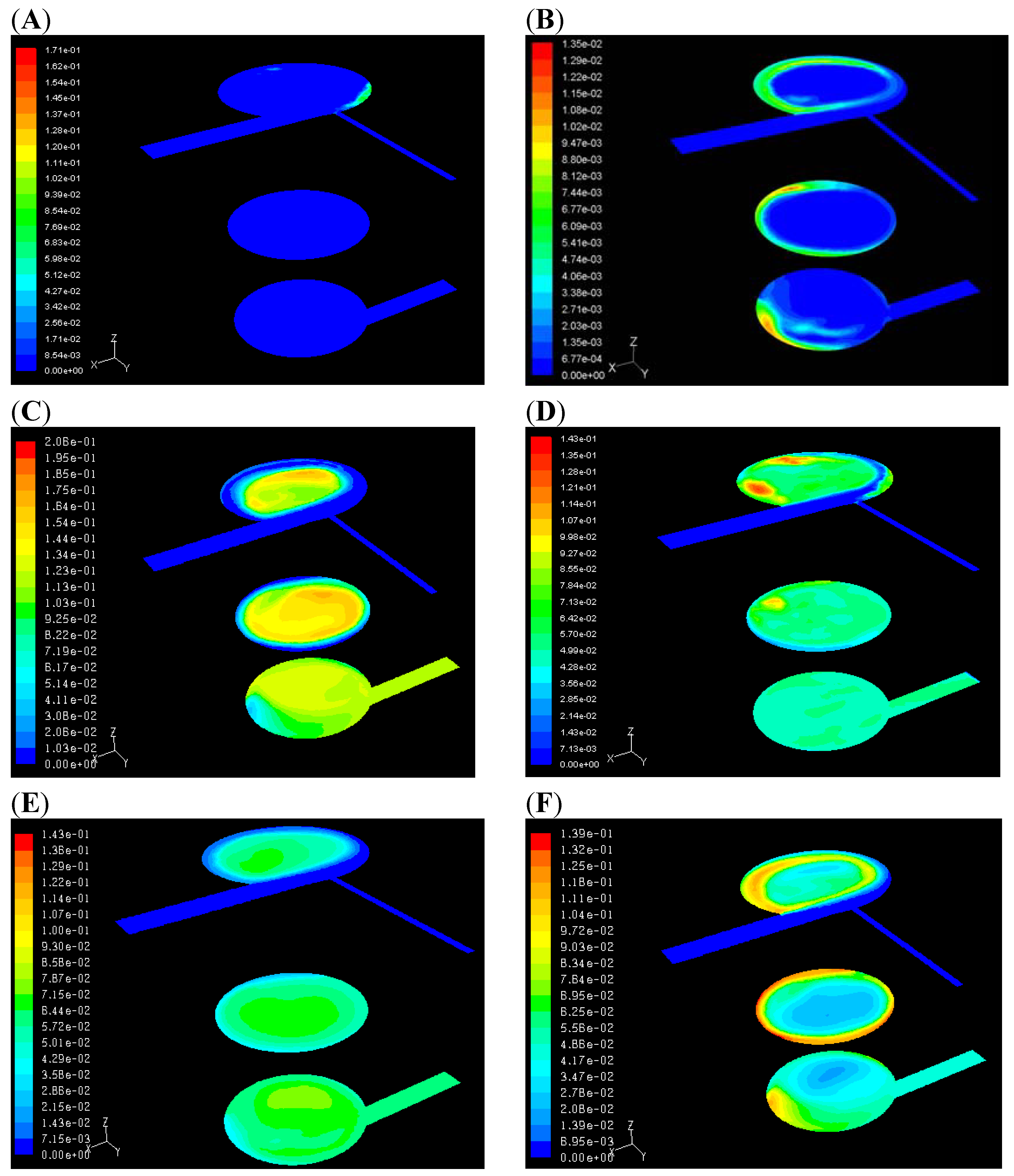
The consequences of such an assumption are clearly exposed by observing the species maps inside the chamber (Figures 2), which are completely different: with Flamelet, the CO and CO₂ production is essentially concentrated at the inlet section and close to the wall, while the “EDC simulation” predicts, at both times, that the CO-CO₂ conversion takes place well downstream of the inlet section.

This means that the Flamelet model predicts complete combustion earlier than the EDC model; in fact, this is confirmed by the combustion efficiency, which is defined by the exhaust anhydrous molar fractions ratio, ${\chi }_i=n_i/\left(n_{\text{tot}}-n_{{\text{H}}_2\text{O}}\right)$:

$$\eta ={\frac{{\chi }_{{\text{CO}}_2}}{{\chi }_{{\text{CO}}_2}+{\chi }_{\text{CO}}+{\chi }_{{\text{CH}}_4}}|}_{\text{outlet}}$$

(5)

Table 5 reports the combustion efficiency values for the three cases.

Figure 2. (A) Flamelet: CO map after 0.03 s; (B) EDC: CO map after 0.03 s; (C) EDC: CO map after 0.05 s; (D) Flamelet: CO₂ map after 0.03 s; (E) EDC: CO₂ map after 0.03 s; (F) EDC: CO₂ map after 0.05 s.

Figure 2. (A) Flamelet: CO map after 0.03 s; (B) EDC: CO map after 0.03 s; (C) EDC: CO map after 0.05 s; (D) Flamelet: CO₂ map after 0.03 s; (E) EDC: CO₂ map after 0.03 s; (F) EDC: CO₂ map after 0.05 s.

Table 5. Combustion Efficiency.

Flamelet at 0.03 s	EDC at 0.03 s	EDC at 0.05 s
0.999	0.27	0.986

Table 5. Combustion Efficiency.

Flamelet at 0.03 s	EDC at 0.03 s	EDC at 0.05 s
0.999	0.27	0.986

The “EDC simulation” needs five residence times to reach a combustion efficiency higher than 0.98, while the “flamelet simulation” needs just three residence times.

Even if the calculated combustion efficiencies are known to be higher than real ones, these orders of magnitude are confirmed by the experiments published by Wu et al. [19], even though those experiments were on much smaller chambers and with oxygen enriched air.

A similar investigation carried out on a smaller chamber (0.25 cm³) [41,42] provided a lower predicted combustion efficiency, η, of 0.8, showing the influence of the higher S/V ratio on η and confirmed the different behavior of the flamelet and EDC models. The fact that even the EDC models predicts an unusually high combustion efficiency is due to the combustion chamber dimensions that are large enough to attain complete reactions.

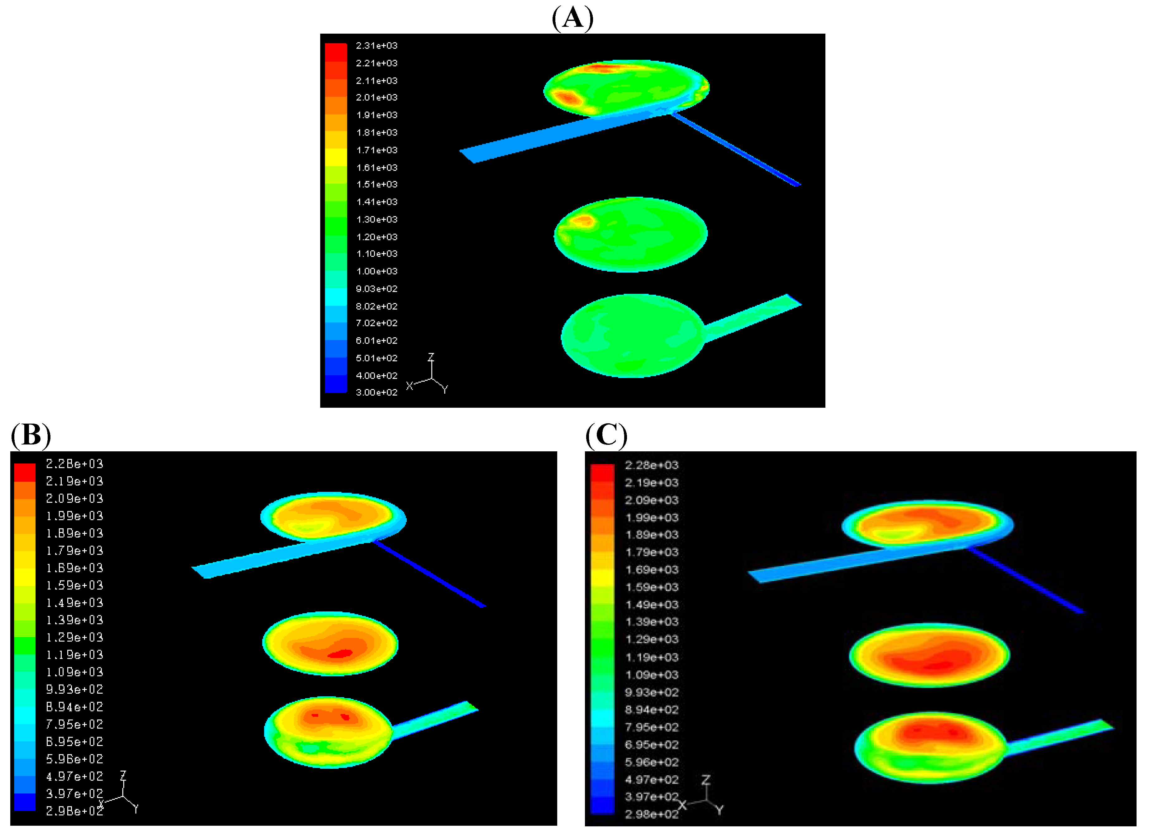
Different species maps, and therefore different combustion efficiencies, lead to different temperature maps, as shown in Figure 3. The “evolution feature” is highlighted in Figures 3 (B and C).

Figure 3. (A) Flamelet: Temperature, t = 0.03s; (B) EDC: Temperature, t = 0.03 s; (C) EDC: Temperature, t = 0.05 s.

Figure 3. (A) Flamelet: Temperature, t = 0.03s; (B) EDC: Temperature, t = 0.03 s; (C) EDC: Temperature, t = 0.05 s.

The “EDC simulation” predicts a hot core and a colder outer zone close the wall, due to the heat losses introduced by the low constant wall temperature of 700 K. Figure 3B clearly displays a noticeable swirling motion as well.

On the contrary, the “flamelet simulation” predicts a more homogeneous temperature field over the entire section, as if the boundary condition at walls were “quasi adiabatic”. Figure 3C shows a weaker swirl too.

The two simulations predict similar maximum temperatures inside the chamber: 2,280 K versus 2,310 K. Temperatures at the outlet section are 1,100 K and 1,270 K.

Experimental support for our conclusions about the inherent physical differences between the two combustion models comes from the comparison between the temperature maps shown in Figure 3 and the time-averaged of CH* chemiluminescence images obtained by [43] (Figure 4). Their results pertain to a combustion chamber smaller than the one studied here (exactly 6 mm diameter and 9 mm length), but, even if only in a qualitative sense, they confirm the general behaviour calculated in the present study.

CH₄ (methane) appears in rich regions of the flame, because it is produced later in methane pyrolysis (after partial CH₂ oxidation has taken place [44] and thus is associated to heat release and can be related with the flame front. This correlation is only approximate though, because it should be remembered that line-of-sight measurements must be interpreted with caution [43]. The time averaged CH* image shows the maximum intensity occurring opposite to the air/fuel injection zone. The central hot bubble is characterized by weaker CH* emission; the zone close to the reactant inlets shows the lowest intensity. In both regions CH* is low because either completely oxidized to CO already, or because methane pyrolysis has not yet begun. Similarly, due to wall flame quenching, no CH* emission was observed in the “dead” layer about 0.5 mm thick close to the wall. Thus, even qualitative, in fair agreement with the mean CH* image, the “EDC mean temperature maps” show that the region of highest gas temperature is located away from the wall and away from the air/fuel injection point, see Figure 3 (B and C).

Figure 4. EDC: Temperature, t = 0.05 s. The chamber wall is the black line.

Figure 4. EDC: Temperature, t = 0.05 s. The chamber wall is the black line.

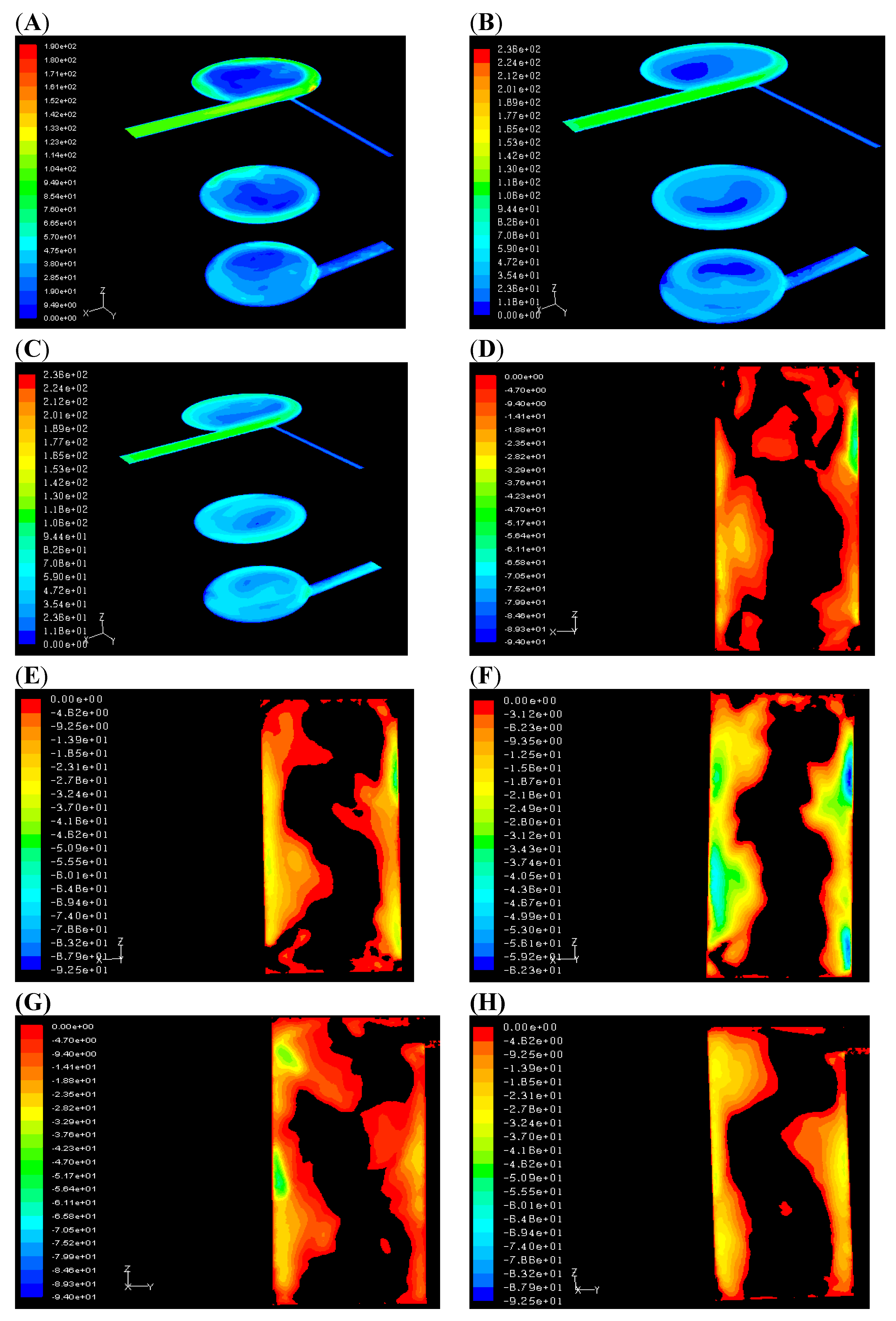
These discrepancies in the prediction of the thermodynamic properties and in the species profiles obviously affect the densities and therefore both the velocity magnitude maps (Figure 5) and the topology of the recirculation zones (Figure 5C–Figure 5I). The zones with the lowest velocity values (Figure 5A–Figure 5C) provide a hint to the complex largest vortex structures inside the chamber.

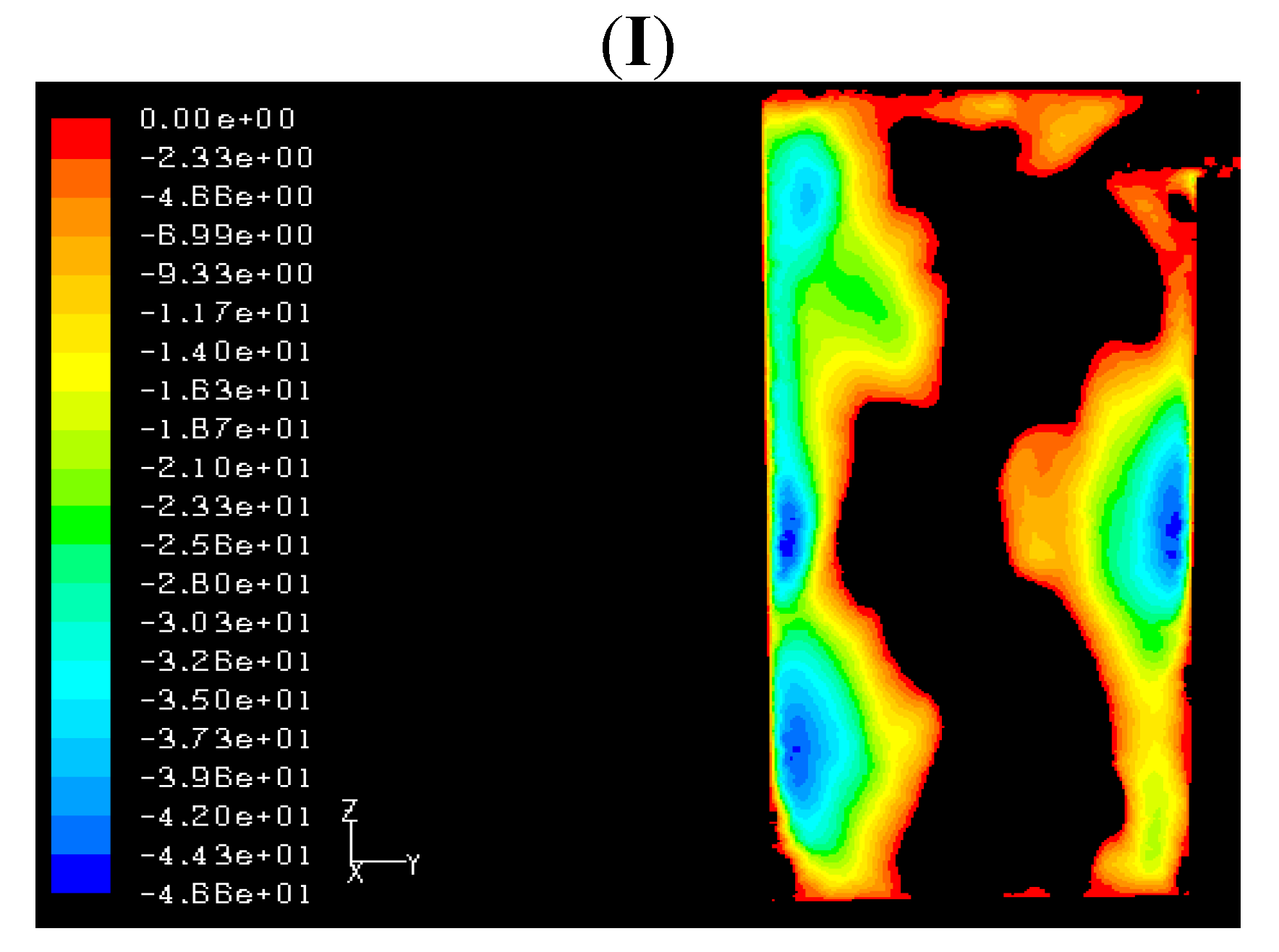
These are more clearly apparent in Figure 5D–Figure 5I that show the mean Z velocity on the “XZ” and “YZ” Planes. These figures indicate only negative Z-velocities, consistent with the “in-out direction” trough the chamber. The black zones (positive Z-velocities) identify the recirculation bubbles in the chamber that promote the mixing process: These regions are quite wide in both simulations but have a more regular shape in the second one (with the EDC model). This flow reversal is a result of the particular shape of the chamber, and in particular is promoted by the outlet section being perpendicular to the cylinder axis and tangent to its external surface (see Figure 1).

Figure 5. (A) Flamelet: Velocity, t = 0.03 s; (B) EDC: Velocity, t = 0.03 s; (C) EDC: Velocity, t = 0.05 s; (D) Flamelet: Z-Velocity, XZ plane, t = 0.03 s; (E) EDC: Z-Velocity, XZ plane, t = 0.03s; (F) EDC: Z-Velocity, XZ plane, t = 0.05 s; (G) Flamelet: Z-Velocity, YZ plane, t = 0.03 s; (H) EDC: Z-Velocity, YZ plane, t = 0.03 s; (I) EDC: Z-Velocity, YZ plane after 0.05 s.

Figure 5. (A) Flamelet: Velocity, t = 0.03 s; (B) EDC: Velocity, t = 0.03 s; (C) EDC: Velocity, t = 0.05 s; (D) Flamelet: Z-Velocity, XZ plane, t = 0.03 s; (E) EDC: Z-Velocity, XZ plane, t = 0.03s; (F) EDC: Z-Velocity, XZ plane, t = 0.05 s; (G) Flamelet: Z-Velocity, YZ plane, t = 0.03 s; (H) EDC: Z-Velocity, YZ plane, t = 0.03 s; (I) EDC: Z-Velocity, YZ plane after 0.05 s.

These differences are confirmed by the dimensionless swirl number, S (defined as the axial flux of swirling momentum divided by the product of the axial flux of axial momentum times the equivalent nozzle radius):

$$S=\frac{{\displaystyle \underset{A}{\int }\rho u_z{u}_{\theta }r\text{d}A}}{r{\displaystyle \underset{A}{\int }\rho u_z^2\text{d}A}}$$

(6)

Table 7 provides the swirl numbers at the inlet plane (Z = 0.055 m) and further confirms the above explanation.

Table 7. Swirl Number.

Flamelet at 0.03 s	EDC at 0.03 s	EDC at 0.05 s
0.47	1.62	0.57

Table 7. Swirl Number.

Flamelet at 0.03 s	EDC at 0.03 s	EDC at 0.05 s
0.47	1.62	0.57

The “EDC simulation” displays different flowfields before reaching steadiness: at 0.03 s it predicts an axial flux of the axial momentum smaller than the swirling momentum, while at 0.05 s it is the opposite. The latter result is obtained by the “flamelet simulation”, two residence times earlier.

6. Conclusions

Scope of this work was the simulation of an air/methane ultramicro-combustion chamber with a nominal thermal power of 2 kW, designed and built at the Sapienza University of Roma. The ultimate goal was that of validating suitable computational tools to design miniature electrical power generators.

Two simulations are reported, both use the LES approach with the WALE SGS model and detailed chemistry, but differ for the combustion-chemistry models: the first uses 67 “flamelets”, while the second uses the EDC model.

Results are reported at two different times: 0.03 s and 0.05 s, that is, almost three and five residence times, respectively. Instantaneous maps of different quantities and a combustion efficiency analysis are provided. The work is focused on the analysis of the different assumptions posited by the combustion models.

Flamelets are calculated by an initial ignition temperature equal to the equilibrium condition and they account for overall transport properties, equal in this case to that of nitrogen which is the species with the highest mass fraction. The EDC model solves the species equations with the local cell properties and explicitly accounts for every transport property.

The analysis starts from the species maps, obtaining the relative combustion efficiency values, and then focuses on the temperature maps to deduce their effect on the velocity fields and then on the swirl numbers. The results presented here lead to the conclusion that while an overall analysis on variables like combustion efficiency and maximum temperature may be carried out by a flamelet model with a substantially lower CPU time than with an EDC model, fundamental physical quantities like heat fluxes, local species concentrations and temperature distribution, and in particular their evolution, are completely mispredicted by Flamelets. This is confirmed by values reported in Table 6 and Table 7, which provide combustion efficiency and swirl number at different times: the ones obtained with the flamelets at 0.03 are in very good agreement with those calculated by EDC at 0.05 s, but the EDC results at 0.03 s are quite different from those at 0.05 s (they show a dynamic evolution absent in the flamelet simulations). A combustion efficiency higher than 0.9 is predicted by both models, but while in the first case this result is caused by the flamelet computation (function only of the fluid dynamics data and not of thermodynamics values), in the EDC model this is due to the fact that the dimensions of the combustion chamber are large enough to allow for the reactions to proceed to completion.

In fact, the “flamelet simulation” predicts complete reactions near the injection section and close to the wall while the second shows more realistic delay times.

Moreover, the difference in the calculated temperature maps is remarkable: the “flamelet simulation” predicts a quite homogenous temperature distribution with the highest value close to the wall, as if a “quasi-adiabatic boundary condition” were imposed on the wall, while the “EDC simulation” predicts -quite on the contrary- a hot core and a colder zone near the wall, respecting the wall heat fluxes due to the constant low wall temperature imposed. We conclude that the EDC approach is more accurate than the flamelets model and it is more suitable to study the evolution phenomena inside combustion chambers of this scale.

A future study will focus on the comparison of the simulation results with suitable experimental data in order to validate the computational model and to obtain useful design information.