Current State of Development of Electricity-Generating Technologies: A Literature Review

Lenzen, Manfred

doi:10.3390/en3030462

Open AccessReview

Current State of Development of Electricity-Generating Technologies: A Literature Review

by

Manfred Lenzen

ISA, School of Physics, A28, The University of Sydney, Sydney, NSW 2006, Australia

Energies 2010, 3(3), 462-591; https://doi.org/10.3390/en3030462

Submission received: 3 February 2010 / Accepted: 10 March 2010 / Published: 18 March 2010

Abstract

:

Electricity is perhaps the most versatile energy carrier in modern economies, and it is therefore fundamentally linked to human and economic development. Electricity growth has outpaced that of any other fuel, leading to ever-increasing shares in the overall mix. This trend is expected to continue throughout the following decades, as large—especially rural—segments of the world population in developing countries start to climb the “energy ladder” and become connected to power grids. Electricity therefore deserves particular attention with regard to its contribution to global greenhouse gas emissions, which is reflected in the ongoing development of low-carbon technologies for power generation. The focus of this updated review of electricity-generating technologies is twofold: (a) to provide more technical information than is usually found in global assessments on critical technical aspects, such as variability of wind power, and (b) to capture the most recent findings from the international literature. This report covers eight technologies. Seven of these are generating technologies: hydro-, nuclear, wind, photovoltaic, concentrating solar, geothermal and biomass power. The remaining technology is carbon capture and storage. This selection is fairly representative for technologies that are important in terms of their potential capacity to contribute to a low-carbon world economy.

Keywords:

electricity generation; global status review; renewable energy; nuclear energy; carbon capture and storage

1. Summary

Electricity is perhaps the most versatile energy carrier in modern economies, and it is therefore fundamentally linked to human and economic development. Electricity growth has outpaced that of any other fuel, leading to ever-increasing shares in the overall mix. This trend is expected to continue throughout the following decades, as large—especially rural—segments of the world population in developing countries start climbing the “energy ladder” and become connected to power grids [1]. Electricity therefore deserves particular attention with regard to its contribution to global greenhouse gas emissions, which is reflected in the ongoing development of low-carbon technologies for power generation.

Why the need for a new assessment of the state of electricity-generating technologies? This work does not aim to replace milestone reports such as the Energy Technology Perspectives [2], or the World Energy Assessment [1]. Its main focus is rather twofold: a) to provide more technical information than is usually found in global assessments on critical technical aspects, such as variability of wind power, and b) to capture the most recent findings from the international literature. As for the second aim, the large majority of a total of 361 references included in this report are more recent than 2004, the year with the most of references cited is 2008, followed by 2007 and 2009 (Figure 1).

Figure 1. Frequency distribution of citations in this report across publication years.

This report was commissioned with the objective of providing an up-to-date snapshot of multiple criteria related to electricity generation, but not with the objective to provide a tool or a basis for multi-criteria decision analysis. It was acknowledged, however, that this study could provide a starting point for further investigation of that subject. Nevertheless, the following observations are made: a multitude of aspects play a role in societal debate in comparing electricity generating options, such as cost, greenhouse gas emissions, radiological and toxicological exposure, occupational health and safety, domestic energy security, employment, and social impacts. Decision-makers will in general weight these aspects differently, and similarly the literature deals with these issues in varying ways. Attempts to quantify the varied consequences of electricity generation in one end-point indicator in order to aid decision-making are fraught with problems, amongst which uncertainty and the discounting are perhaps the two most extremely challenging, despite the fact that relative rankings of electricity generation options did not change substantially during the course of the ExternE project (Figure 2 in [3]). First, on a purely scientific basis, and from a statistical point of view, in many cases the large uncertainties associated with impact and damage parameters preclude decision-making [4]. For example the very-long-term consequences of radioactive waste disposal are almost impossible to reliably predict, given the very long time horizons, and the lack of practical experience with operating repositories. Also the systematic incompleteness of impact pathways covered means that central values and ranges for damages can in principle not be stated. Second, whenever impact lifetimes are long such as global warming, long-term habitat transformation, or radioactive releases, monetary comparisons of future damages are extremely sensitive with regard to the discount rates assumed, leading to the complete failure of conventional cost-benefit analysis (for example, applying an even very small discount rate to time spans of the order of nuclear waste half lives would set the present value of future damages practically to 0). This is in addition to the difficulty of arguing an intergenerational discounting process, when the preferences of future humans are not even known (see the interesting contributions in the literature on discounting, such as [5,6,7,8,9,10,11]). It is hence increasingly accepted that a purely technical approach aiming at objective and unique assessment of risk is infeasible, and that risk has legitimate and important ethical dimensions that must be considered and managed [12].

A scientific-quantitative approach alone does not provide a basis for comparisons and decisions. Philosophy and lifestyles come into play in determining preferred energy strategies (Section 3.1 in [3]). Here, a whole range of criteria applies, such as spatial and temporal immediacy, ability to control or trust in decision-makers, fear and dread, knowledge and familiarity, risk profile (probability and magnitude). The formation of public perception is further complicated by the fact that media and political campaigns often comment more rapidly and decisively on contentious issues, thus reaching the public more effectively than sources of less biased factual information. For example nuclear energy is often portrayed and hence perceived as an invisible danger under the control of a few, and associated with military use, suppression of information, and high accident risk [13,14]. On the other hand of the spectrum, large hydroelectric dams are associated with the forceful resettlement of large numbers of people, and the destruction of archaeological heritage and biodiversity [15]. Similarly, but perhaps surprisingly, offshore wind power is at times strongly opposed for environmental reasons, often based on beliefs that are “stunningly at odds” with the scientific literature [16]. Whilst public acceptance must play a role in decision-making, it is important that the public forms their opinion on the basis of complete, transparent and balanced information. Unfortunately, in this respect, the literature examined in this report revealed examples of bias and omission.

This report covers eight technologies. Seven of these are generating technologies: hydro-, nuclear, wind, photovoltaic, concentrating solar, geothermal and biomass power. The remaining technology is carbon capture and storage. This selection is fairly representative for technologies that are important in terms of their potential capacity to contribute to a low-carbon world economy. Currently, only nuclear and hydropower generate significant low-carbon portions of global electricity (Figure 2).

Figure 2. 2006 regional and fuel split of world electricity generation (compiled from data in [17]).

This report does not cover supply-side and end-use efficiency and conservation measures, and it does not cover some future electricity-generating technologies such as fuel cells, wave, current and tidal power, and nuclear fusion, though it does provide a starting point for further study. Further, it deals with combined heat and power, and storage technologies only where they have a major bearing on the generation performance of the seven technologies listed above. Finally, it does not deal with transmission issues common to all technologies. These omissions shall not necessarily indicate that these technologies could not contribute significantly to a future energy mix. For example, efficiency improvements have led to drastic decreases in the carbon intensity and other pollutant characteristics associated with fossil power plants [18,19], although continuing efficiency improvements face barriers in that they are less visible and popular than new technologies, and dispersed, with support difficult to organise at a large scale [1]. The efficiency of power transmission is an important area in terms of innovations such as High-Voltage DC long-range transmission systems, superconductors, and wide-area monitoring systems. Fuel cells are seen as the key technology to a future hydrogen economy [20]. Storage of all types (pumped hydro, molten salts and rocks, electric vehicle fleets), and combined heat and power are essential components improving the integration and capacity credits of variable renewable energy resources at high renewable penetration rates, in that they enable the temporal and spatial relocation of excess power [21,22,23,24,25]. However, marine renewable devices are behind their terrestrial counterparts in terms of maturity [26], and the commercialisation of nuclear fusion appears to be at least four decades away [27].

Within the scope of this work, technologies and their contribution to world electricity demand and emissions abatement have been appraised more or less in isolation. In fact, there are potential large synergies between power technologies and with non-power technologies, for example the cost-reducing effect of carbon storage on oil recovery, combined heat and power, multiple-purpose plants (for example biorefineries for fuel reforming, power, and hydrogen production), the reduction of renewable output variability through portfolio diversity, or the adaptation to renewable output variability through changes in the demand system such as matched loads. In order to gain a complete understanding of energy supply and emissions abatement potential, the technologies described here have to be appraised from a systems perspective, by investigating whole strategies and scenarios, integrated not only across all electricity generating technologies, but also across other energy carriers such as liquid fuels and heat, across end-use characteristics, and across demand management and conservation options.

In order to calculate the mitigation potential of all sources (Table 1), the IPCC SRES A2 scenario was taken as a reference scenario. The mitigation potential is the difference in cumulative emissions between the IPCC SRES A2 scenario and a modified SRES B1 scenario (Figure 3) where the respective technology assumes its economic or resource potential, according to the literature. The A2 scenario family represents a differentiated world. It is characterized by low trade flows, relatively slow capital stock turnover, and slow technological change. The A2 world "consolidates" into a series of economic regions. Self-reliance in terms of resources and less emphasis on economic, social, and cultural interactions between regions are characteristic for this future. Economic growth is uneven and the income gap between now-industrialized and developing parts of the world does not narrow [28]. The central elements of the B1 future are a high level of environmental and social consciousness combined with a globally coherent approach to a more sustainable development. Heightened environmental consciousness might be brought about by clear evidence that impacts of natural resource use, such as deforestation, soil depletion, over-fishing, and global and regional pollution, pose a serious threat to the continuation of human life on Earth.

Figure 3. Modified SRES B1 scenario chosen as the alternative scenario for calculating mitigation potentials. The difference between the B1 variant used here and the IPCC SRES scenario (inset; [28]) is the timing of fossil-fuelled power. The relatively sudden post-2040 increase in renewable power in the IPCC scenarios could not be reconciled with bottom-up projections, which see renewable sources become significant earlier than 2040. Pre-2006 are actual historical data.

In the B1 storyline, governments, businesses, the media, and the public pay increased attention to the environmental and social aspects of development. Technological change plays an important role. At the same time, however, the storyline does not include any climate policies. Particular effort is devoted to increases in resource efficiency to achieve the goals stated above. Incentive systems, combined with advances in international institutions, permit the rapid diffusion of cleaner technology [29].

These scenarios were chosen because A2 comes close to a business-as-usual case where the fuel mix does not change dramatically, while B1 emphasises renewable energy sources in the energy mix, as well as a reduced electricity demand (33% lower at 2100 relative to A2) due to efficiency and conservation measures (Figure 3). The B1 scenario is in reasonable agreement with the International Energy Agency’s ACT Map and BLUE Map scenarios [2] regarding 2050 electricity demand and renewable share (see Figure 8). 2100 emissions reductions from all sources are about 17 Gt CO₂ per year, which again agrees well with the ACT Map and BLUE Map scenarios that project CO₂ reductions from power generation to be 14 and 18 Gt CO₂, respectively (see Figure 9). Assuming a low-demand scenario such as the B1 favours renewable technologies because they can achieve large generation shares at moderate deployment growth.

Future potentials are constrained by various factors such as grid integration (wind), resource base (hydropower and uranium resources), geographical mismatch (carbon capture and storage, and biomass), and cost (photovoltaic and concentrating solar). Mitigation potentials hence include dynamic effects due to future fuel mixes, and hence materials for constructing new power systems becoming less and less carbon-intensive (compare with results in [29] and [30]). Dynamic effects affect all technologies equally, since they draw on materials and inputs from a more or less carbon-intensive background economy. However, the mitigation potential estimates do not take into account any rebound effects that might happen because of redirecting technology-driven savings of electricity cost to the consumer into other spending areas. Finally, scenarios are not forecasts, they are possible storylines. In principle, that and to which extent scenario outcomes will actually occur is unknown, and no probability is placed on such occurrences.

The 2100 time horizon chosen for mitigation potentials in this report is longer than most projections found in the literature, which cover the period up to 2030 or 2050. The choice for a longer time horizon was made: a) bearing in mind the inertia and lifetime of climate change, and the resulting relevance of long-term emissions, and b) taking into account that some more recently matured technologies need long lead times for deployment. Notwithstanding the above, projections towards to the end of this century are best guesses, that are based on our understanding of existing society, technology and infrastructure. Much infrastructure stock is going to be turned over until 2100, and new technologies and synergies, new resource discoveries, as well as societal and policy restructuring may result in mitigation outcomes that are substantially different from the estimates offered here. In short: Much can and will happen before 2100.

In this report, electricity costs are reported as levelised cost, that is as the constant (discounted to present values) real wholesale price of electricity that recoups owners’ and investors’ capital costs, operating costs, fuel costs, income taxes, and associated cash flow constraints. They exclude costs for transmission and distribution [31]. Levelised cost may differ from sales prices, because of profits or losses. The figures reported here are averages over plant types and vintages, and over locations with varying resource endowments and demand profiles. Actual cost for particular plants may be different from the cost given here. Levelised electricity costs are strongly determined by the competitive landscape, in particular the extent and nature of regulation, subsidisation and taxation, primary fuel (coal, gas, uranium) prices, and future carbon pricing. Whilst under government regulation operators are able to transfer costs and risk to consumers and taxpayers, this is not the case in deregulated electricity markets, where high interest rates lead to investors favouring less capital-intensive and therefore less risk-prone power options. Electricity cost figures reported here refer to the financial and regulatory environment at the time of publication of the various references. An attempt has been made to select studies close to one base year, for the sake of comparability. The year 2006 was chosen as the base year, because for this year a reasonable number of cost studies could be located. Note that since this year, commodity prices have undergone changes that could affect levelised electricity cost. An example for this effect is the costs quoted in Table 3 of [32] which are somewhat higher than those quoted in Table 1. Subject to these qualifications, this literature review has yielded the results shown in Table 1.

Table 1. Current state of development of electricity-generating technologies (representative characteristics).

**Table 1.** Current state of development of electricity-generating technologies (representative characteristics).
Technology	Annual generation ^a (TWh_el/y)	Capacity factor ^b (%)	Mitigation potential ^c (GtCO₂)	Energy requirements ^d (kWh_th/kWh_el)	CO₂ emissions (g/kWh_el)	Generating cost (US¢/kWh)	Barriers
Coal	7,755	70–90		2.6–3.5 ^e,f	900 ^e,f	3–6 ^g	Greenhouse gas emissions
Oil	1,096	60–90		2.6–3.5 ^h	700 ^h	3–6 ^g	Resource constraints
Gas	3,807	≈ 60		2–3 ^e,f,i	450 ^e,f,i	4–6 ^g	Fuel price
Carbon capture and storage	-	n.a.	150–250 ^j.k	2–2.5 + 0.3–1 ^l	170–280 ^f,l,m	3–6 + 0–4 ^n,o,p	Energy penalty, large-scale storage, late deployment
Nuclear fission ^q	2,793	86 ^r	> 180	0.12 ^s	65 ^s	3–7 ^g,t	Waste disposal, proliferation, public acceptance
Large hydro	3,121	41	200–300 ^u	0.1 ^v	45–200 ^v,w	4–10 ^g,t	Resource potential, social and environmental impact
Small hydro	≈250	≈50	≈100 ?	n.a.	45 ^v	4–20 ^g,t,x	Resource potential
Wind	260 ^y	24.5	≈450–500	0.05 ^z	≈65 ^z,aa	3–7 ^g	Variability and grid integration
Solar-photovoltaic	12 ^ab	15	25–200 ?	0.4/1–0.8/1 ^ac	40/150 – 100/200 ^ac	10–20 ^g,t,ad	Generating cost
Concentrating Solar	≈1	20–40	25–200 ?	0.3 ^h	50–90 ^h	15–25 ^g,t,ae	Generating cost
Geothermal	60	70–90	25–500 ?	n.a.	20–140 ^af	6–8 ^ag	Uncertain field capacity
Biomass	240 ^ah	60 ^ah	≈ 100	2.3–4.2 ^ai	35–85 ^ai	3–9 ^t,ah	Efficiency, feedstock availability, cost

^a [13]; ^b Energy deployment E and load factor λ are related to the power deployment P as E = P × 24 h × 365 d × λ; ^c difference between the IPCC SRES A2 and a modified SRES B1 scenario where the technology assumes its economic or resource potential; ^d kWh_th are counted as fossil energy only, hydropotential, nuclear energy and ambient energy are excluded; ^e [3,4,5]; ^f full life-cycle; ^g [18]; ^h [4]; ⁱ Figure 2 in [7]; ^j [12]; ^k Table TS.3 in [1]; ^l [8]; ^m 75 g/kWh with enhanced oil recovery, [9]; ⁿ base cost + cost for capture, transport, and storage, 0 value indicates net economic benefit in enhanced oil recovery; ^o [6]; ^p Table 1 in [10]; ^q thermal reactors only; ^r [11]; ^s [2,14]; ^t [15], Tabble 2-17; ^u [16]; ^v [17]; ^w [19]; ^x highly scale- and site-dependent, [20,21]; ^y [22]; ^z [23], excludes variability impacts; ^aa [24]; ^ab [25]; ^ac [17], lower values for conceptual plants, higher values for operational plants; ^ad [26]; ^ae [27]; ^af [28], 20 for binary-cycle plants (emissions embodied in the plant); ^ag [29]; ^ah [13,30]; ^ai [5], assumes existing agricultural lands.

Carbon capture and storage is seen as a potentially significant CO₂ mitigation route because it would allow retaining major parts of current electricity generation infrastructure and build on existing knowledge and practices. Capture technologies are well understood but remain to be demonstrated at a large commercial scale, which is not expected before 2020. Costs additional to those of current fossil power are expected to be between 1 and 3 US¢/kWh. Retrofitting of existing plants is seen as too expensive, and mandating “capture-ready” plants is recommended. A major barrier is the so-called energy penalty of 20%–25%, which is due to a reduction in plant efficiency around 10%, and to energy requirements of the capture process. The energy penalty implies the need to deploy significant additional capacity solely to enable the capture process, and also comparatively high residual CO₂ emissions in the order of 170–270 g CO₂/kWh. Considering existing storage sites and their distances to major CO₂ sources, the potential contribution of carbon capture and storage to this century’s global mitigation effort is estimated at between 150 and 250 Gt CO₂. Uncertainties about the magnitude of long-term leakage of CO₂ from subsurface reservoirs exist, and setting up the legal and regulatory framework for “pore space ownership” and long-term responsibility is a challenge. Politically, carbon capture and storage is criticised because of its potential to divert attention away from the development of inherently low-carbon generation technologies.

Nuclear power is seen as a mature technology, with many reactor-years of experience, and modern reactors exhibiting a high degree of safety. Nuclear power currently contributes 14% of global electricity generation. The majority of nuclear reactors are thermal reactors, and this is expected to remain the case in the mid to long term. Current average capacity factors of 86% are amongst the highest of all technologies and levelised costs are competitive between 4 and 7 US¢/kWh. Future Generation-IV reactor designs such as fast reactors and compact liquid metal or salt reactors, as well as advanced fuel cycles promise advances in reactor fuel utilisation, enhanced proliferation resistance, reduction of nuclear waste volumes, and passive safety, however no design satisfies all criteria, and deployment is not expected to start before 2030. Nuclear power is a low-carbon technology, with current emissions of around 65 g CO₂/kWh. Even if future ore grades declined to 0.01%, and emissions increased to around 130 g CO₂/kWh, nuclear power would still be considered low-carbon. Further, uranium resources are sufficient for current operations to continue throughout this century, and based only on current reasonably assured and inferred resources and their grades, nuclear power would be able to make a significant contribution to global mitigation of at least 180 Gt CO₂. The future of nuclear power appears to be strongly influenced by public perception and concerns about safety, waste disposal, and proliferation risk. In this respect, some major barriers for nuclear power are its association with military utilisation, non-disclosure of sensitive information, the lack of proven very-long-term waste storage, and the indeterminate state of much of the spent fuel. Further, there exists some lack of information about currently mined ore grades, and the state of rehabilitated uranium mines. Finally, at least in the US and much of Europe, the nuclear supply chain faces restrictions in form of skilled labour shortages and supplier market contractions, which may affect the quick re-activation of nuclear building programmes, as a large number of existing reactors are nearing their end of life.

Hydropower deploys 870 GW and contributes more than 3 PWh annually, or 17% of global electricity generation, and it therefore dominates the renewable technology suite. 90% of this electricity is generated by large hydro dams, with the remainder generated by small, mostly run-of-river plants. The long-term resource of large hydro is limited because most large rivers have already been dammed. Further, large dam projects have been plagued by public opposition because of their social and environmental impacts (displacement of people, land-use change, sedimentation, eutrophication, river bed scouring, habitat disturbance), which is not the case for small run-of-river plants. On the other hand, dams have multiple uses such as flood control, water supply and recreation. Future expansion is probably limited overall to doubling or tripling current generation, which corresponds to a mitigation potential of 300–400 Gt CO₂. The decay of submerged biomass, especially in tropical reservoirs, can be a significant source of methane and CO₂, estimated at 40–200 g CO₂/kWh. Hydropower has excellent start-up and load-following capability, and is therefore able to provide both base and peak load. Average capacity factors are between 40% and 50%. Levelised cost for large hydro are competitive at between 5 and 10 US¢/kWh, but not for small hydro projects. The latter currently cost up to 20 US¢/kWh, and therefore mainly occupy niche markets for remote power supply. Hydropower plants have long life times of up to 100 years, so that after upfront capital costs have been recouped, long-term operating costs are amongst the lowest of all generating technologies.

Wind power is the second-strongest-growing of all technologies examined in this report, with recent annual growth rates of about 34%. The technology is mature and simple, and decades of experience exist in a few countries. Due to strong economies of scale, wind turbines have grown to several megawatts per device, and wind farms have now been deployed off-shore. The wind energy industry is still small but competitive: 120 GW of installed wind power contributes only about 1.5% or 260 TWh to global electricity generation at average capacity factors of around 25%, and levelised costs between 3 and 7 US¢/kWh, including variability cost. The technical potential of wind is larger than current global electricity consumption, but the main barrier to widespread wind power deployment is wind variability, which poses limits to grid integration at penetration rates above 20%. Life-cycle emissions for wind power alone are amongst the lowest for all technologies, however in order to compare wind energy in a systems view, one needs to consider its low capacity credit: Adding emissions from fossil balancing and peaking reserves that are required to maintain overall systems reliability places wind power at about 65 g/kWh. Wind power’s contribution to emissions abatement is potentially large at 450–500 Gt CO₂ for this century.

Photovoltaic power is the strongest-growing of all technologies examined in this report, with recent annual growth rates of around 40%. One of the largest markets was remote power supplies, in particular for developing-country communities that are not connected to electricity grids, but this has changed during recent years as developed countries have embarked on rebated residential-roof deployment programs. Photovoltaic modules are deployed dispersed at small scale, which makes it difficult to ascertain globally installed capacity, which is estimated at about 9 GW. Assuming an average capacity factor of 15%, global generation is 12 TWh. The capacity credit of photovoltaic power depends on demand characteristics: in sunny locations with high summer peak loads for example for air conditioning, photovoltaic power can achieve capacity credits of up to 80%. Due to the energy-intensive manufacturing of crystalline cells, life-cycle emissions are variable but in general relatively high at around 100 g/kWh. The technical potential is larger than current global electricity consumption, but the main barrier to widespread deployment is high cost: These have decreased substantially during the past decades, but are still amongst the highest of all technologies included in this report at between 10 and 20 US¢/kWh. Whether photovoltaic power will be able to make a significant contribution to future electricity generation is dependent on the continuation of past learning curves, which have recently slowed down. Future contributions to emissions abatement are hence rather uncertain, but based on existing scenarios could be anywhere between 25 and 200 Gt CO₂.

Concentrating solar power, sometimes also referred to as solar-thermal power, was strongly pursued in the 1980s and 1990s, but renewed interest has emerged recently. At present only 0.4 GW are operating at large-scale plant levels, generating some 1 TWh annually, using mostly parabolic troughs, but also tower, dish and Fresnel designs. Concentrating solar plants integrate well with conventional thermal plants, for example as fuel savers. The average capacity factor is at least 20%, but can reach beyond 40% when heat transfer fluids with high thermal capacity are used for hourly storage. Combined with storage, the capacity credit of concentrating solar power is higher than that of photovoltaic power, with sunny locations and high summer peak loads achieving credits of more than 80%. Life-cycle emissions are in the mid range between 50 and 90 g/kWh. The technical potential is larger than current global electricity consumption, but the main barrier to widespread deployment is high cost: These have decreased substantially during the past decades, but are still amongst the highest of all technologies included in this report at between 15 and 25 US¢/kWh. More concentrating solar plants are currently proposed, in part for large-scale “sun-belt” visions, and it is expected that cost decrease substantially with renewed R&D. Future contributions to emissions abatement are rather uncertain, but based on existing scenarios could be anywhere between 25 and 200 Gt CO₂.

Geothermal power has been utilised for power generation since 1920. Globally it only accounts for 10 GW deployed, but some countries derive a major proportion of their electricity from geothermal reservoirs. Geothermal plant efficiency depends on the quality of the resource. Low-temperature resources require one or two flashing processes in order to utilise steam turbines. Electricity generation has been growing slowly at about 4% annually, and is currently about 60 TWh at 70% average capacity factor, but capacity factors up to 90% are considered possible. Geothermal boasts the largest technical potential of all technologies, however resource development can be slow due to a combination of uncertain field capacity and high drilling cost, requiring a step-wise development process, with results obtained from a small number of wells before the field is further expanded. This procedure is recommended in order to avoid mismatches between field and plant capacity, but it can entail an uncertain environment for investors. Completed plants are near-competitive at levelised cost between 6 and 8 US¢/kWh. Life-cycle emissions are quite variable between 50 and 120 g/kWh, depending on whether a binary or open cycle plant is used, and on whether new geothermal vents are created during field exploration. Future contributions to emissions abatement are rather uncertain, but based on technically possible scenarios could be anywhere between 25 and 500 Gt CO₂.

Biomass power is secondary to uses of biomass for liquid transportation fuels, but it is currently used economically in dedicated applications such as pulp and sugar industries. Its global deployment is only around 50 GW generating 1.5%, or some 240 TWh of electricity. Currently, biomass plants combust agricultural and forestry residues, and waste. The long-term potential of these types of feedstock is lower than that of dedicated energy crops, but the latter have preferential usage for biofuels. Dedicated biomass plants are small in size because of locally limited feedstock availability and transportation requirements, and hence suffer from dis-economies of scale. Further technical challenges are in developing gasifier, boiler and turbine designs that can handle variable- and low-quality biomass and deal with the resultant pollutant deposits and corrosion. Co-firing is regarded as the preferred option, but at biomass shares above 10% it leads to efficiency losses and requires structural changes to plant components such as feeders. Levelised costs are competitive at between 3 and 5 US¢/kWh. Capacity factors are lower than those for coal-fired power plants, at around 60%. The main barrier for large-scale biomass exploitation is the potential compromisation of food, fodder and biodiversity objectives. Meeting all constraints, future potentials have been estimated to be around 3%–5% of world electricity generation. At this level, using suitable feedstock with low life-cycle emissions, and assuming that no land needs to be cleared, biomass power would mitigate about 100 Gt CO₂. Biomass power in combination with carbon capture and storage has the potential for net sequestration of CO₂, however carbon capture is not economical in small biomass plants. Biomass power may be a co-product in future biorefineries.

2. Rationale

The aim of this report is to identify the current state of development of eight technologies. Seven of these are generating technologies: hydro-, nuclear, wind, photovoltaic, concentrating solar, geothermal and biomass power. The remaining technology is carbon capture and storage.

This report portrays technologies in terms of a number of characteristics, which will allow easy yet comprehensive comparison for decision-making. In particular, this review covers for each technology

–: its technical principle,
–: the total potential of its global energy sources,
–: its capacity factor and capacity credit,
–: life-cycle characteristics, such as kWh-specific greenhouse gas emissions, or embodied energy, over the lifetime of the installations,
–: the scale at which the technology is currently deployed,
–: the contribution it currently makes to global electricity supply,
–: the cost of its current electricity output,
–: the extent of subsidisation by governments (in a separate section), and
–: technical and other challenges.

This report includes technologies that are quite diverse and of varying degrees of complexity. For those technologies that are more complex and where crucial details are less known (carbon capture and nuclear power), the technical detail section is more detailed than for well-known and relatively simple technologies (hydro and wind). The section on wind contains detailed explanations on variability and capacity credit. This report also includes some technologies that are currently undergoing research, and which may exist in form of demonstration plants. Their inclusion positions this research to provide a basis for future research which will look at possible future development trajectories of these generating technologies under various assumptions.

Finally, three notes of caution: First, a few of the literature items pointed out that during the last few years a number of even high-level reference documents on technologies have been superseded by updated information within a year or little more. Naturally, this qualification applies to this review as well: It reflects the understanding at the time of writing. Second, some of the references contain value statements or recommendations for what are preferable technologies for combating climate change. Some of these statements are documented here, but they do not reflect the opinion of the author, but the content of the respective references. Third, this report was prepared with a budget of 20 person-weeks. This means that the work referenced here is neither a necessarily representative nor exhaustive selection of the literature on electricity-generating systems, but that instead the information gathering, processing and presentation was restricted by a timeframe of roughly 2 person-weeks per technology section.

3. Introduction

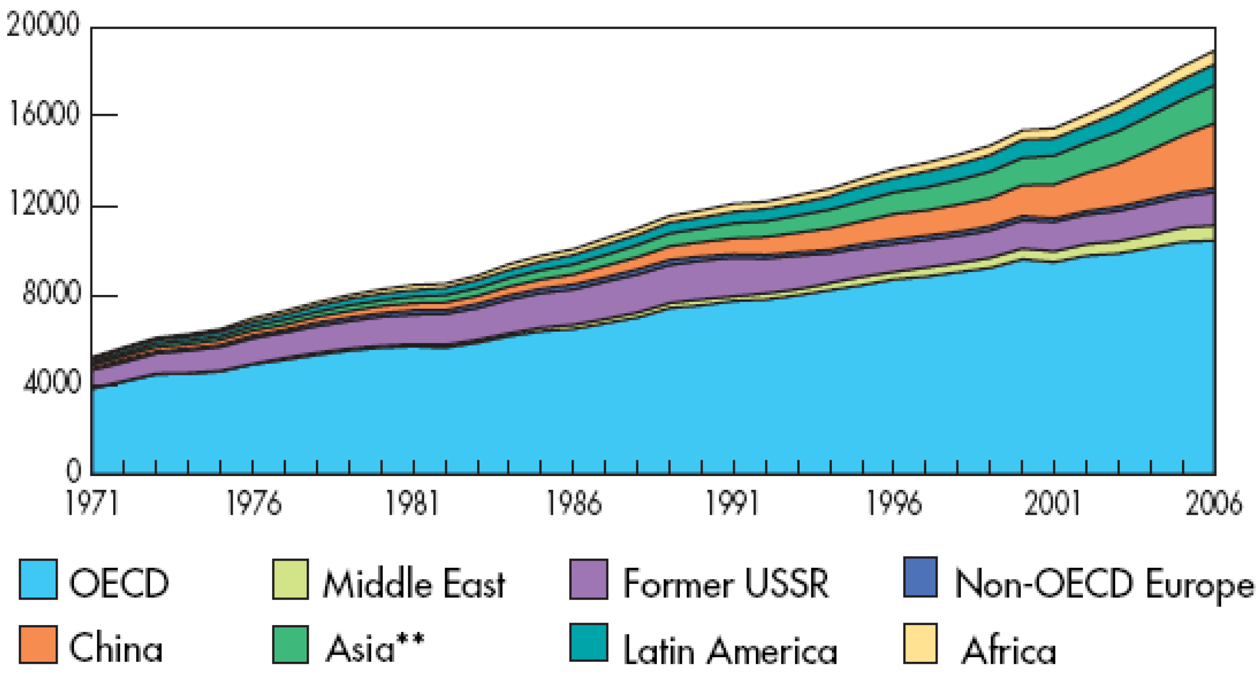
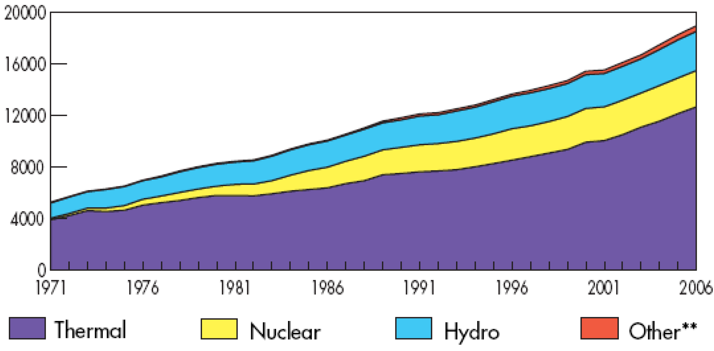
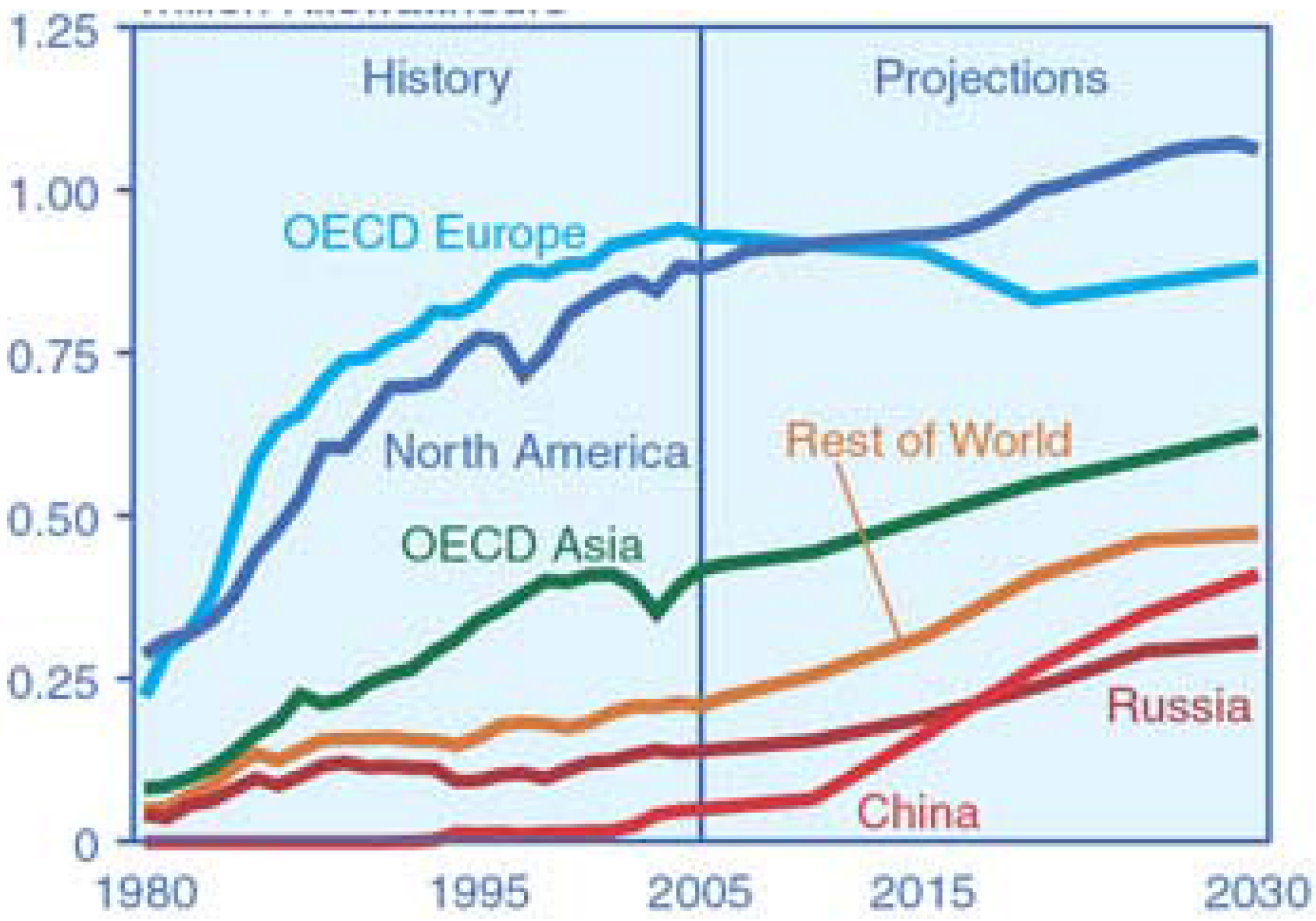
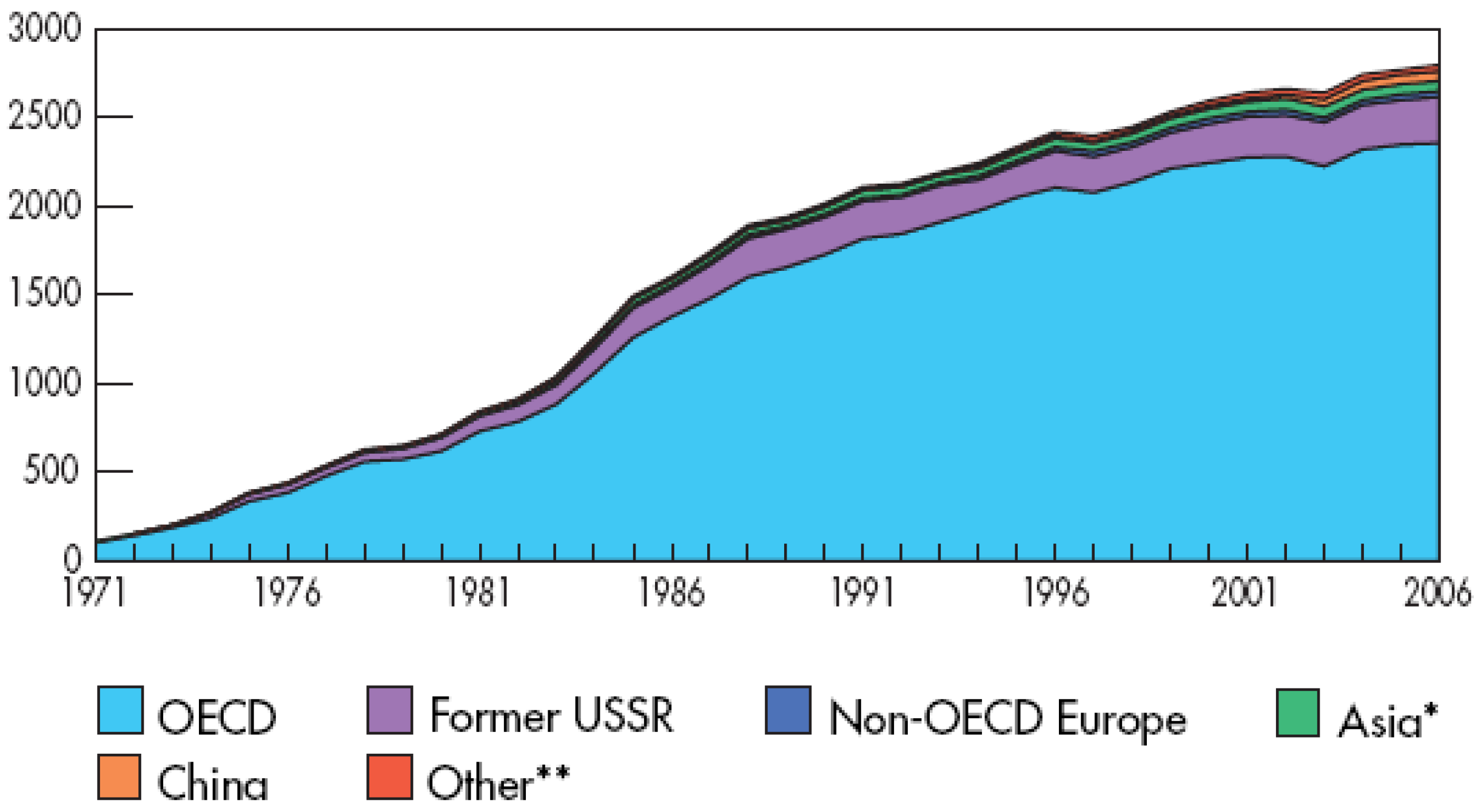
3.1. Role of Electricity in World Energy Needs

Electricity is perhaps the most versatile from of modern energy: It is extensively used throughout all areas of final consumption (light, heat, electrical and electronic devices), with the exception of transport. A strong correlation between per-capita electricity consumption and the Human Development Index exists (Figure 4). Maza and Villaverde [60] summarise studies of causality between per-capita electricity consumption and per-capita GDP, concluding that in many cases growth in electricity consumption causes GDP growth, and less so the other way round.

Whilst the shares of other energy carriers have remained constant or have declined (coal 13.3% (1973), 8.6% (2006); oil 48.1%, 43.1%; gas 14.4%, 15.3%; biofuels and waste 13.2%, 12.9% [17]), electricity has nearly doubled its share in final consumption between 1973 and 2006 [17]. This is the case for both OECD countries and the rest of the world. China, Asia and the OECD contributed most to the growth in electricity consumption (Figure 5). Electricity now accounts for 16.7% of energy needs worldwide (up from 9.4% in 1973), second only to oil for transport (26%). This can be expected to grow to current OECD standards (20.3%, up from 11.4% in 1973) as more areas of the developing world are connected to power grids.

In 2006, 67% of worldwide electricity was generated using fossil fuels (41% coal and peat, 5.8% oil, and 20.1% gas), 14.8% nuclear energy, 16.0% hydropotential, and 2.3% renewable sources [17]. Since 1973, nuclear power has seen the largest increase (up from 3.3%), mainly at the cost of oil (down from 24.7%) and to a lesser extent hydro (down from 21%). Whilst coal remained about constant (slightly up from 38.3%), gas could also nearly double its share (up from 12.1%; see Figure 6). This decline of oil is not necessarily due to a direct technological competition between nuclear and oil [63], but rather because of energy security concerns after the oil price shocks, and also because of advances in gas turbine technology (efficiencies, capital cost, peak- and base-load ability) leading to the rapid growth of natural gas in the energy portfolio. Today, the different fuels service different segments of the electricity market: whilst nuclear, coal are responsible for centralised base load provision, gas and oil are able to dominate peak, back-up and dispersed non-grid generation [63].

Figure 6. Evolution of electricity production (TWh) by fuel. Other includes geothermal, solar, wind, combustible renewables & waste, and heat. © 2008 OECD/IEA, reproduced from [17] with permission.

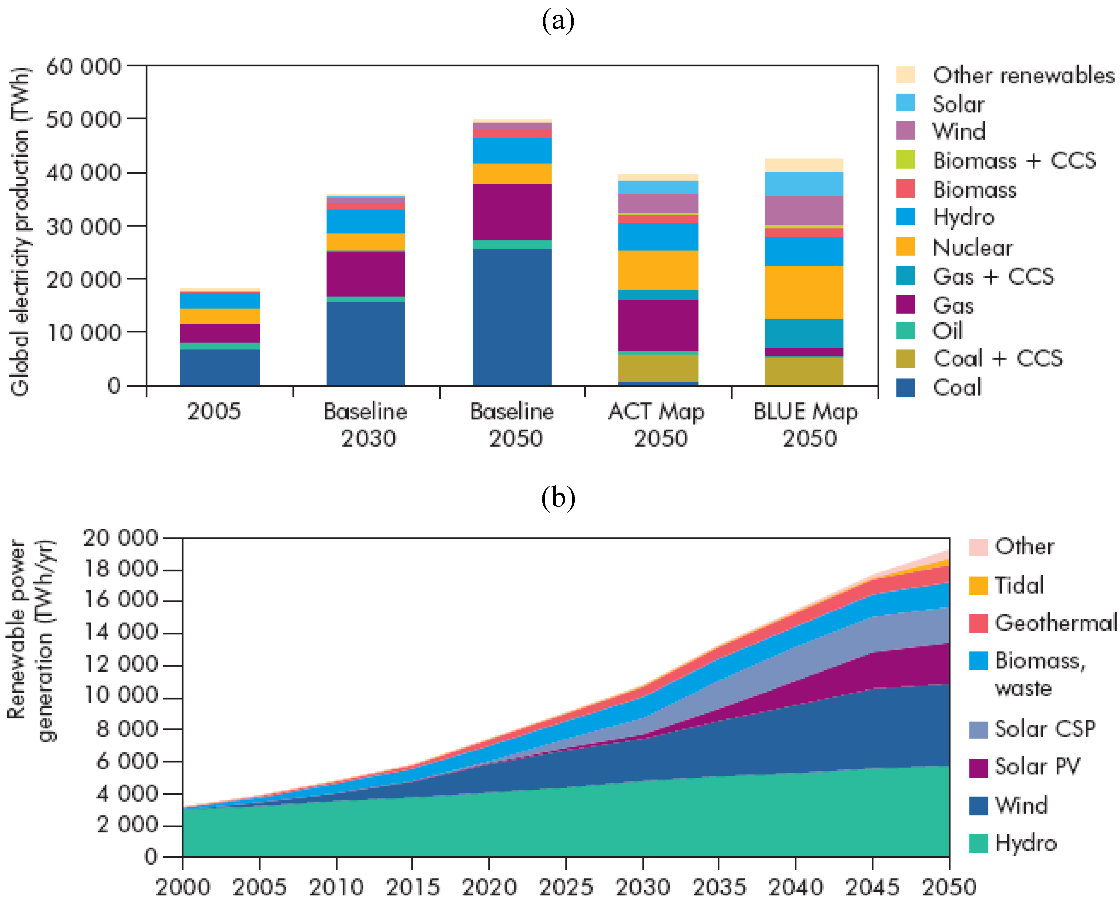
3.2. Demand Projections and Scenarios

Total primary energy supply (TPES) is projected to grow during the next few decades, but this growth is projected to be somewhat slower than the growth between 1973 and 2006, where TPES almost doubled from 257 Exajoules (10¹⁸ J, EJ) to 493 EJ. The 2030 TPES is expected to be between 660 and 740 EJ (alternative and reference policy scenarios) [17]. The share of the OECD will further shrink from 47.1% in 2006 (down from 61.2% in 1973) to less than 40% in 2030, at the cost of China (1973 7%, 2006 16.2%, 2030 20%) and the rest of Asia (1973 5.7%, 2006 11.3%, 2030 14.2%). All other regions are projected to maintain their shares. In the IEA’s reference scenario, gas and coal are projected to expand at the cost of mainly oil, but also nuclear energy. In the alternative policy scenario, renewable see the main proportional increase, followed by gas and nuclear, at the cost of oil and coal. None of the percentage changes projected by the IEA until 2030 is greater than 4%, so changes are rather moderate.

Fossil fuels are also seen as the main energy source at least until 2030 in the World Energy Outlook, also published by the IEA [64], but the moderate projected changes stand in stark contrast to the IEA’s overall assessment, which sees the world’s energy system at a crossroads, with “shocking consequences for the global climate of policy inaction”, and where the need for low-carbon energy supplies “is nothing short of an energy revolution”. This may be explained by the dilemma that is posed by the reality of emission targets to prevent dangerous climate change on one hand, and the reality of long-term locked-in fossil infrastructure and the reluctance for early retirement of significant capital investment. Unsurprisingly, the IEA’s World Energy Outlook admits that a 450 ppm scenario represents a huge challenge, where for example low-carbon sources have to supply 40% of all electricity generation by 2030. It is not known whether this scenario is achievable, but major spending shifts towards low-carbon energy supplies, and removing US$310b of subsidies on energy consumption are measures that will have to be taken in any case.

Figure 7. World electricity generation outlook (PWh), by region (left) and by fuel (right) (after [65]).

In their International Energy Outlook, the Energy Information Administration of the U.S. Department of Energy projects electricity generation to continue to be the fastest growing source of energy [65], and to nearly double between 2005 and 2030 from 17 to 33 PetaWatt-hours (PWh, 10¹² kWh; Figure 7). Non-OECD countries’ strong growth in personal affluence will drive strong economic growth that will translate into electricity demand, and these countries are projected to overtake OECD countries in total generation by nearly 50%. Coal is projected to increase its share in generation from 41% to 46% due to high oil and gas prices. Nuclear power’s share is projected to decrease slightly, but generation is projected to grow by 50% nevertheless, mostly in non-OECD Asia, often driven by needs for energy portfolio diversification and energy security, and higher fossil fuel prices. This is in contrast to the IEA’s reference scenario, where nuclear power’s shares experiences larger decreases, mainly because of assumptions about China’s nuclear program (a detailed comparison of scenarios can be found in [66]). Renewables’ combined output is projected to increase only slightly at under 2% per year, and its combined share is even expected to decrease slightly if gaps in electricity cost persist in the absence of carbon pricing.

Perhaps the most detailed technology scenarios are available from the International Energy Agency’s Energy Technology Perspectives [2]. The IEA provides two scenarios (the ACT Map and the BLUE Map, Figure 8, both described as challenging) that see atmospheric CO₂ concentrations reduced to 520 ppm and 450 ppm (Figure 9), respectively, resulting in temperature changes between 2 °C and 3 °C. In addition to end-use efficiency and conservation, these scenarios consider the deployment of all technologies covered in this report.

4. Carbon Capture and Storage

Because of its compatibility with the current energy supply infrastructure and well understood health, safety and environmental practices, carbon capture and storage is seen as the only technology available to mitigate CO₂ emissions at a large scale in a world where large-scale fossil fuel usage will remain a reality well into the 21^st century [33,64]. However, it is also acknowledged that capture and storage alone will not be able to stabilize CO₂ concentrations [67]. There were no operational carbon capturing power plants at the time of writing (only industrial separation plants), but CO₂ was being injected at three sites worldwide. However, post- and pre-combustion technologies are seen as economically feasible (Table TS.1 in [33]), and around 20 carbon capture and storage pilot projects have been proposed [68], but large-scale feasibility has yet to be demonstrated. At the 2008 Hokkaido summit, G8 countries endorsed the IEA’s recommendation to commit these large-scale projects by 2010, with a view for deployment by 2015 [69]. This deployment has to be accompanied by a legal and regulatory framework that creates appropriate incentives for the adoption carbon capture and storage technologies [2]. Retrofitting existing plants with capture technology appears too costly [70]. A recommended strategy that provides for accelerated uptake is therefore to mandate “CCS-ready” new power plants that provide for immediate carbon capture retrofit [2].

The IPCC Special Report (p. 22 in [33]) notes the importance of assessing carbon capture and storage in a systems view with an appropriate boundary, that is including the energy requirements and emissions associated with all capture, transport and storage processes. IPCC estimates 10%–40% or more energy compared to a plant without capture, leading to only 80%–90% of CO₂ emissions being captured on a net basis (for a detailed study see [41]). The parasitic effects of the capture process on overall plant efficiency and CO₂ balance are referred to as the energy penalty. This is seen as one of the main barriers for large-scale deployment of the technology, because it requires the deployment of a significant fraction of total electricity demand just for the capture of CO₂. It also means that specific greenhouse gas emissions per kWh are larger than those of some renewable power technologies or nuclear and hydropower [71]. Another important uncertainty is the lack of experience with underground storage and potential leakage under potential future deployment scales, and the associated risks [67,72,73]. However, these risks are not necessarily perceived by the public [74].

In the following, three main technologies for carbon capture and storage are compared, because these are seen as closest to commercial application ([75]; see Figure 10). All technologies involve the separation of CO₂, H₂ or O₂ from a bulk gas stream; solid fuels are either combusted or gasified. There are differences in terms of net plant efficiency and avoided CO₂ emissions ([76]; Table 2.5 in [77] provides an overview of advantages and disadvantages), generally favouring integrated-gasifier and natural gas combined cycle technology. Large variations occur in cost estimates, because of varying assumptions and system configurations [41]. Appropriate benchmarking of capture and storage technologies requires a careful definition of a reference system [78].

Figure 10. Schematic representation of methods for carbon capture (after [70]).

Many studies describe additional energy needs of capture plants in terms of percentage decreases in efficiency (1 – η_CCS/η_reference). Rubin et al. [41] suggest a measure of energy penalty EP = η_reference/η_CCS – 1, but also acknowledge that neither characterises the entire life cycle of capture and storage plants (Footnote 3 in [41]). In this report, we understand energy penalties in the sense of Life Cycle Assessment (LCA), that is as energy requirements stemming from the entire upstream plant life-cycle [39]. Energy penalties are larger than efficiency reductions.

4.1. Potential of Resource

The potential of carbon capture and storage is determined by the geographical relationship between large stationary emitters of CO₂ (the majority of them power stations) and their proximity to suitable storage sites [33]. Individually small and mobile sources are unsuitable. Comparing the global distribution of major stationary emitters and the locations of prospective sedimentary basins, a potentially good correlation emerges.

IEA estimates that carbon capture and storage in electricity generation and industrial processes could be responsible for 15%–20% of emissions reductions (5–10 Gt CO₂ per year) in a range of scenarios [69]. The IPCC lists current large plants emitting a total of 13.5 Gt CO₂ per year (Table TS.2 in [33]), and quotes 2.5–5 Gt CO₂ per year (10% of annual emissions) by 2020, and 5–40 Gt CO₂ per year (20%–45% of annual emissions) by 2050. In simulations by Riahi et al. (Table 2 in [43]; [79] is essentially the same paper), carbon capture starts expanding relatively late (only after 2050; Figure 10), and avoids 3–10 Gt C per year by 2100. On a cumulative basis, these estimates are in the range between 15%–55% of the mitigation effort until 2100, or 150–250 Gt C (Table 1 in [43]) and 200–2,000 Gt CO₂ [70], which coincides with, or is at the lower end of estimates for storage capacity (see Section 3.5). The ranges reflect uncertainty and differing assumptions between future scenarios—mainly about technological learning (Figure 11 in [43]) and prices for avoided carbon [80]. Moreover, the above figures are derived from least-cost optimisation, and do not include real-world market imperfections and barriers to development. Long-term cost of carbon capture and storage have been estimated from historical cost trends and learning curves (a classical learning curve describes decreasing cost trends with a power function y = a x^–b) for related technologies [81], to be around 1–3 US¢/kWh (Table 1 in [41], [38], Table SPM.3 in [70], and [33]). Rubin et al. [41] review cost of electricity under many varying assumptions and operating modes. Moreover these costs will depend on discount rates (Section 6.5 in [82]). Biomass combustion and carbon capture applied in conjunction can achieve a net removal of CO₂ from the atmosphere, albeit at higher capture cost of about 8 US¢/kWh [33]. Net removals can be used to offset the more essential uses of hydrocarbon fuels such as in air transport. In addition to electricity, large carbon capture and storage facilities could also be used in the future to produce hydrogen for dispersed residential, commercial and transport applications.

The general consensus appears to be that in principle, carbon capture and storage represents a viable mitigation route and competitive candidate for future deployment starting around 2015, provided that long-term containment of CO₂ in underground reservoirs can be proven. However, by then, major structural decisions will have been made about large-scale investment in new electricity-generating technology for coming decades, and it is unclear whether carbon capture and storage will be sufficiently developed for large-scale deployment at that time. If not, the development of other low-carbon generating technologies would be preferable. Therefore, some authors see the world at a crossroads in this respect, and argue that a decision for continual reliance on fossil fuels with the prospect of carbon capture and storage will entrench the direction of long-term future energy strategies, and divert attention away from much-needed development of low-carbon technologies [71,73,74].

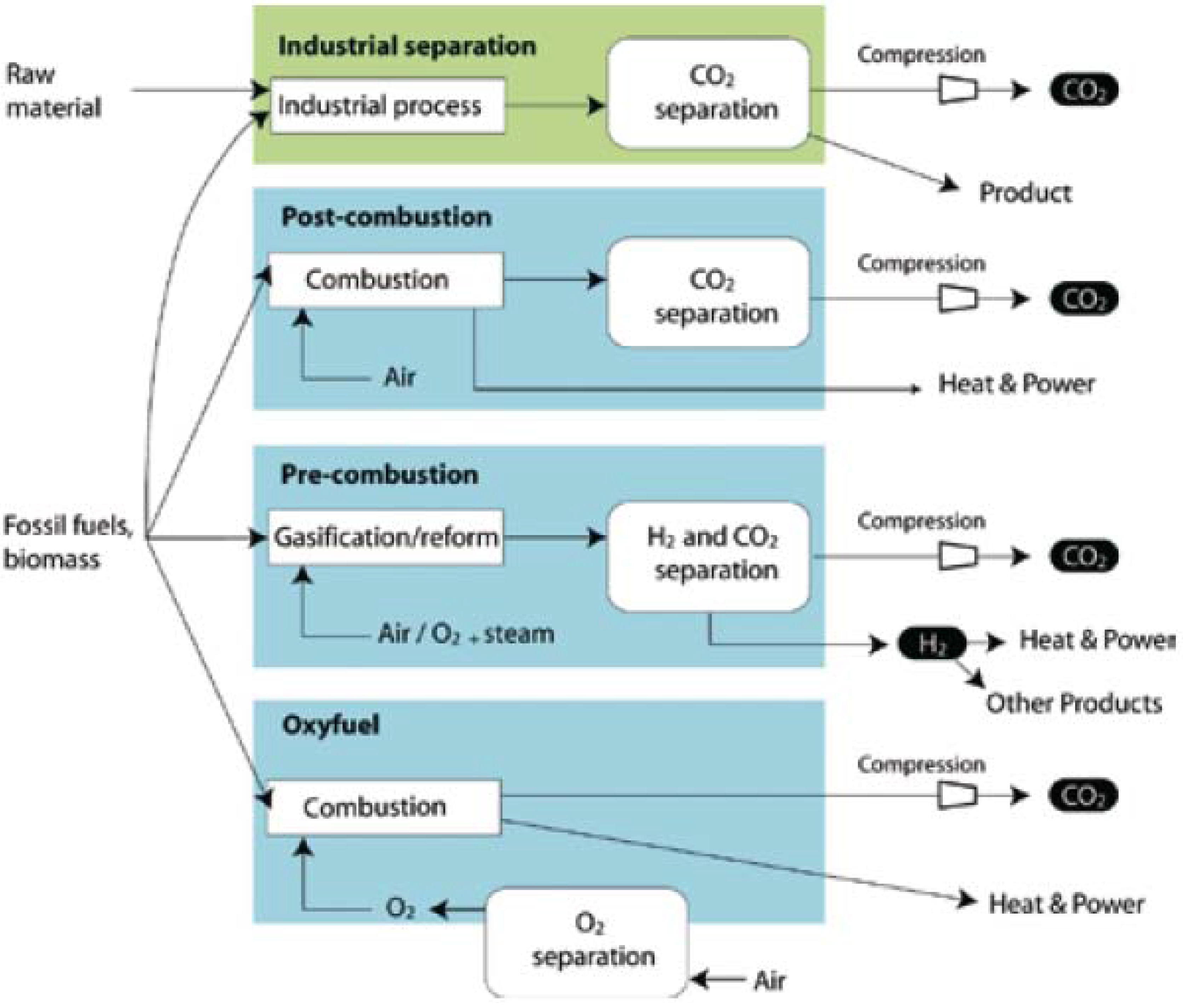
4.2. Post-combustion Capture

4.2.1. Technical principle

Post-combustion carbon capture is the most mature of the three technologies described in the following. It can be applied to pulverised-coal and integrated gasifier combined-cycle power plants. There is no gasification, complex chemical processes, new high-temperature materials required as in the remaining two technologies, but this comes at a cost of a relatively high energy penalty with possibly higher cost. The most commercially advanced method for post-combustion carbon capture (because of existing applications for gas purification) is wet scrubbing of CO₂ (a wet scrubber treats a polluted gas stream by bringing it into contact with a scrubbing liquid, for example by spraying or by forcing through a pool; wet scrubbers are able to remove particulate matter and/or gases) with aqueous amine solutions at about 50 °C [amines are organic compounds containing nitrogen that are derivatives of ammonia, with hydrogen atoms replaced by organic compounds such as alkyl and aryl groups. Most widely used for the removal of CO₂ and H₂S from process or flue gas streams are aqueous monoethanolamine (MEA), diglycolamine (DGA), diethanolamine (DEA), diisopropanolamine (DIPA) and methyldiethanolamine (MDEA)]. The solvent is then regenerated for re-use by heating to 120 °C, and thus recycled continuously. The removed CO₂ is then compressed for geological storage. Post-combustion plants are characterized by thermal efficiencies that are 8%–10% (coal) and 6%–8% (natural gas) below that of corresponding plants without capture (Figure 2 in [82], and Table 1 in [68], [83]). About half of this decrease is due to the additional steam required for the solvent regeneration, a third is due to the need to compress CO₂, and the remainder due to additional power for solvent recycling (Figure 2 in [82], and [75]). In principle, the entire flue gas stream (of which CO₂ constitutes 3%–15%, whilst the major part is nitrogen from air) could be captured and stored, however prohibitive energy and financial cost render this alternative not viable [33].

4.2.2. Capacity and load characteristics

Capture operates at the same load as the generation of electricity.

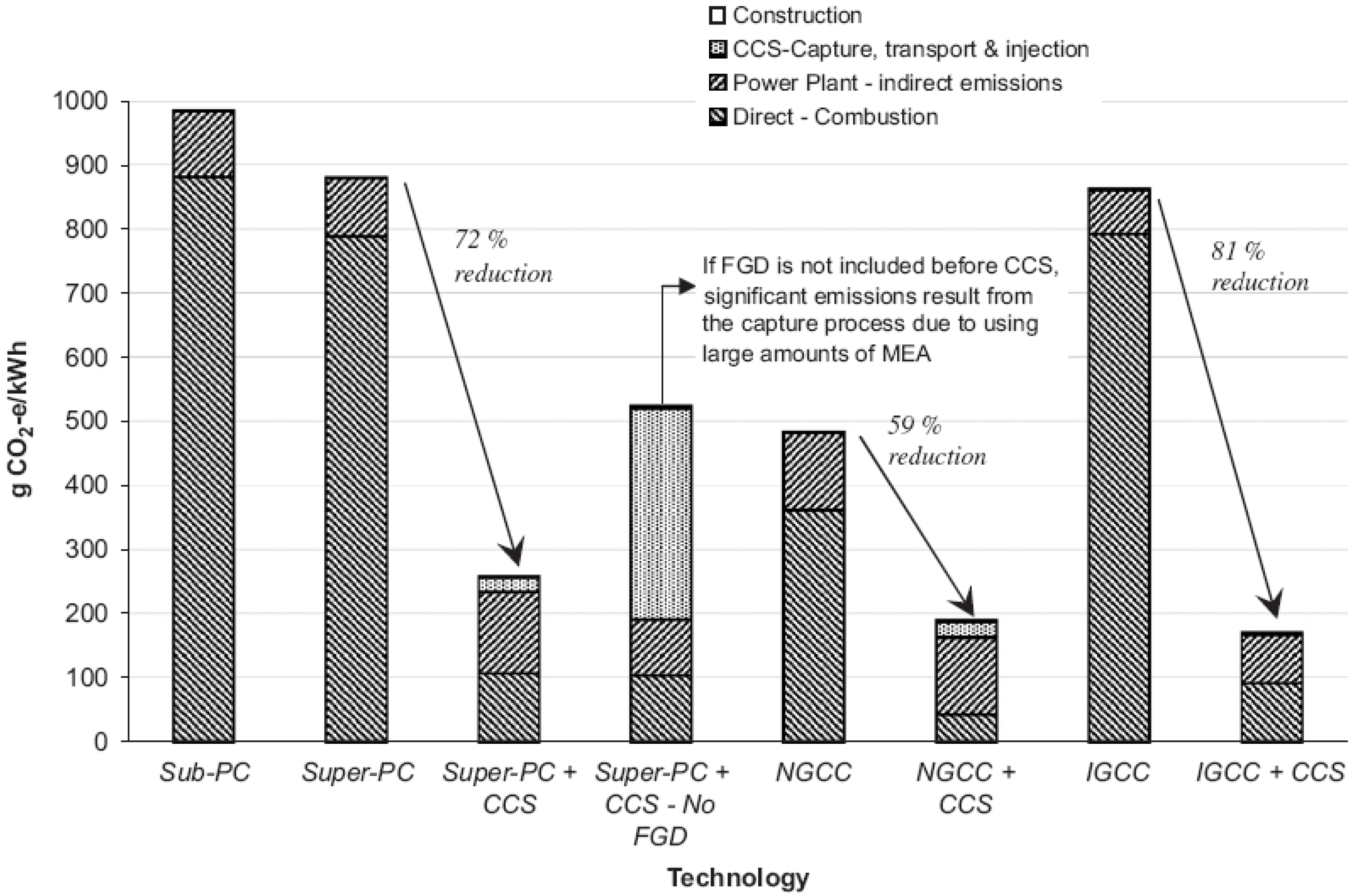
4.2.3. Life-cycle characteristics

The review by Odeh and Cockerill [39] studies of life-cycle energy requirements and CO₂ emissions of carbon capture and storage technologies. They cite a study by Spath and Mann [84] on a pulverised coal and natural gas combined cycle plant, where post-combustion capture and storage decreased the life-cycle CO₂ emissions from 847 to 247 g/kWh, and from 499 to 245 g/kWh, respectively. Viebahn et al. [71] reports comparable values of 274 and 200 g/kWh, respectively. Odeh and Cockerill [8] finds that coal transport distances have a larger influence on life-cycle characteristics than CO₂ transport distances. For post-combustion capture applied to pulverised coal and natural gas combined cycle plants they report life-cycle energy requirements of 2.8 and 2.2 kWh_th/kWh_el, and specific CO₂ emissions of 255 and 200 g/kWh, respectively. Pehnt and Henkel [72] states values of around 200 g/kWh as well. The heating of the solvent for recycling represents a substantial proportion of the energy requirements of post-combustion capture (Section 2.2.2 in [85]). Capture, transport and storage of CO₂ contribute less than 10% to overall life-cycle CO₂ emissions. This is confirmed in a detailed LCA study of a post-combustion system in Norway by Hertwich et al. [40], however Pehnt and Henkel [72] arrive at values of less than 1% for this stage. Hertwich et al. [40] studied a combined-cycle power plant equipped with post-combustion carbon capture and storage used for enhanced oil recovery. Allocating the energy and emissions overheads of CO₂ transport and injection to the oil recovery, they arrive at greenhouse gas emissions for the power plant of only 75 g/kWh. The specific emissions of the capture and compression system amount to 54 g/kWh and 33 g/kWh, respectively (the specific emissions of the transport and injection stages cannot be recovered from the results since they refer to a m³ of oil recovered). This value may be seen as the lower limit of reductions to be expected from carbon capture and storage technologies.

Figure 11. Comparison of greenhouse gas emissions from power plants equipped with carbon capture systems (PC – Pulverised coal, FGD – Flue gas desulphurisation, NGCC – Natural gas combined cycle, IGCC–Integrated gasifier combined cycle). Carbon capture for PC and NGCC via post-combustion using MEA as solvent, for IGCC pre-combustion (Selexol process). Note that in the absence of FGD, life-cycle emissions increase dramatically, because SO₂ reacts with the MEA solvent, rendering it unusable for further downstream CO₂ capture. © 2008 Elsevier, reproduced with permission from [39].

4.2.4. Current scale of deployment

At the time of writing there was no power plant operating with post-combustion carbon capture. The UK government has initiated a competition to identify a 300–400 MW post-combustion technology to capture CO₂ off a pulverised-coal power plant.

4.2.5. Cost of electricity output

The main contributor to overall cost of carbon capture and storage is the carbon capture process [86]. For the post-combustion technology, atmospheric-pressure absorbers and the solvent recycling attract higher capital cost compared to pre-combustion designs. The difference to no-capture plants is estimated at about 2 US¢/kWh (Table 5 in [82], and Table 1 in [68]), between 1.5 and 2.5 US¢/kWh (Table 1 in [71]), or between 1 and 3.5 US¢/kWh (Table 1 in [41]). Rubin et al. also find weak economies of scale (Figure 4 in [41]), and stronger dependence of cost on coal quality (Figure 5). Costs will remain high throughout the initial development period [80].

4.2.6. Technical challenges

Major challenges are the reduction of cost for carbon capture in existing pulverised coal plants, and the reduction of energy requirements for solvent recycling. Efficiency losses due to carbon capture could be offset by improvements in overall plant efficiency. Here, a critical issue is the development of materials that allow higher-efficiency (-temperature) steam cycles (Table 4 in [75]).

At present carbon capture technologies experience significant economies of scale, which means that they do not match well with decentralized energy supply, for example combined heat and power plants, or biomass power plants [86].

4.3. Pre-combustion Capture

4.3.1. Technical principle

Pre-combustion capture can only be effectively utilized in newer power plant designs, such as Integrated Gasifier Combined Cycle (IGGC) or natural-gas-fired combined cycle (NGCC) plants. Contrary to its name, pre-combustion capture still involves some form of chemical oxidisation, such as partial combustion or reformation [68]. Pre-combustion capture operates in two stages: In the first reactor the fossil fuel is gasified to synthesis gas (syngas). Gasification is a process that reacts coal, oil or biomass at high temperatures with a controlled amount of oxygen and/or steam and thus converts them into carbon monoxide and hydrogen. Gasification produces a gas mixture called synthesis gas or syngas, which can be combusted more efficiently than the original fuel. Gasification of fossil fuels is currently widely applied at large scales, using a wide range of raw materials (even plastic waste), in order to generate electricity. A second (“shift”) reactor contains catalyst beds facilitating a water-gas shift reaction, producing CO₂ and hydrogen. The reversible gas phase water-gas shift reaction reaches equilibrium very quickly in a gasifier. In essence, a limited amount of oxygen or air is introduced into the reactor to allow some of the organic material to be “burned” to produce carbon monoxide and energy (C + ½ O₂ → CO), which drives a second reaction that converts further organic material to hydrogen and additional carbon dioxide (CO + H₂O ↔ CO₂ + H₂). Adding steam and reducing the temperature shifts the equilibrium towards CO₂. The CO₂ is then dissolved to leave a hydrogen-rich fuel gas. This fuel gas can be used in the same plant to generate electricity, or it can be used for other applications in a future hydrogen economy.

An advantage of pre-combustion in comparison to post-combustion is that CO₂ is produced at high pressures, thus avoiding some need for pressurisation for subsequent transport and injection. On the other hand, pre-combustion capture is associated with efficiency losses because: (a) some of the CO which is shifted to CO₂ would normally pass the turbine and contribute to electricity generation, and (b) heat transfer coefficients are higher for hydrogen-rich fuels than for natural gas or syngas, so that turbine inlet temperatures have to be reduced to the operational range of the turbine components, leading to a reduced temperature difference and efficiency. Additional losses are incurred for solid and liquid fuels because of the need for gasification. Pre-combustion plants are characterized by thermal efficiencies that are 12%–14% below that of plants without capture ([87], Table 1 in [68]). About half of this decrease is due to additional energy required for the shift reaction, and the remainder equally due to additional power for CO₂ capture processes and CO₂ compression (Figure 2 in [82]).

A true pre-combustion method is hydrocarbon dissociation of natural gas, where methane is dissociated via CH₄ → C + 2H₂. The solid carbon can be stored for future use, or embedded in products such as electrodes or graphite. One problem with this technology is that the dissociation reaction needs high temperatures (>1,200 °C) in order to break the methane bonds. Another issue is that potential cost reductions for the produced H₂ fuel through sales of the C product have limited scope: Significant production of hydrogen would yield in the order of several 100 Mt C, whereas at present only 15–20 Mt C are embedded in all carbon products worldwide. Advanced carbon fibre materials for construction and manufacturing could become new future carbon markets [88].

4.3.2. Capacity and load characteristics

Capture operates at the same load as the generation of electricity.

4.3.3. Life-cycle characteristics

The gasification process is carried out at elevated pressures (30–70 atm), thus allowing the release of CO₂ from the solvent at above-atmospheric pressures and the recycling of the solvent without heating. The energy requirements of pre-combustion capture are therefore significantly lower than those of post-combustion capture [68]. The review by Odeh and Cockerill [39] studies of life-cycle energy requirements and CO₂ emissions of carbon capture and storage technologies. They cite a study by Viebahn et al. [71] on an IGCC plant, where pre-combustion capture and storage decreased the life-cycle CO₂ emissions to 240 g/kWh. Odeh and Cockerill [39] find for pre-combustion capture applied to integrated gasifier combined cycle plants, life-cycle energy requirements are 2.6 kWh_th/kWh_el, and specific CO₂ emissions are 167 g/kWh. This value is confirmed by Pehnt and Henkel [72]. Capture, transport and storage of CO₂ contributes negligibly to overall life-cycle CO₂ emissions (see [72], and Figure 11).

4.3.4. Current scale of deployment

At the time of writing there was no power plant operating with pre-combustion carbon capture.

4.3.5. Cost of electricity output

The loss in efficiency constitutes an important indirect electricity cost. The difference to no-capture plants was estimated at about 1.5–3.5 US¢/kWh, depending on the initial fuel (Table 1 in [68]), or between 1 and 2 US¢/kWh [71], or between 1 and 2.5 US¢/kWh (Table 1 in [41], and Table 5 in [82]). IGCC plants are still in their development, and estimates of electricity costs are therefore more uncertain. Rubin et al. [41] also find weak economies of scale (Figure 4), and stronger dependence of cost on coal quality (Figure 5, see also Section 6.7 in [82]). For NGCC plants, a major influence on cost and performance are gas prices, which have in the recent past led to significant reduction in load factors (Figure 1 in [41], and Sections 6.4 and 6.6 in [82]). Costs will remain high throughout the initial development period [80]. The cost for hydrogen utilization in a more diversified hydrogen economy depend on the requirements for hydrogen transport and storage infrastructure, and are rather uncertain at present [86].

4.3.6. Technical challenges

Future development of high-temperature turbine components are needed to shift peak cycle temperatures from 600 °C to up to 750 °C [68], and thus allow for higher conversion efficiencies using hydrogen-rich fuel gases.

The geographical characteristics of carbon capture and storage and widespread hydrogen usage do not coincide well: Hydrogen distribution is costly and favours decentralisation, whilst carbon capture is capital-intensive and favours centralisation, and storage is dependent to suitable sites [88].

4.4. Oxyfuel capture

4.4.1. Technical principle

Oxyfuel combustion describes the fuelling of a power plant with an oxygen-enriched gas mix instead of air. Most of the nitrogen in the input air is removed in an air reactor, resulting in 95% oxygen. In order to avoid excessive flame temperatures from firing with pure oxygen, some recycled flue gas is added to the gas input. This flue gas also serves to carry the fuel gas into the boiler and provide convective heat transfer throughout the boiler. Oxyfuel combustion produces approximately 75% less flue gas than air-fuelled combustion, and exhausts CO₂ (80%) and H₂O. Boiler sizes are therefore much reduced [89], and the CO₂ can therefore be more easily separated and sequestered. However, because of the energy and economic costs of producing oxygen, an oxy-fuel power plant is less efficient than a traditional air-fired plant (thermal efficiencies around 10% below that of plants without capture, see Figure 2 in [82]). Remaining pollutants in coal to be combusted such as N and S compounds must be removed during compression of the CO₂.

Chemical-looping combustion is a new technology that applies the idea of combusting the fuel with O₂ instead of with air, but in contrast to oxyfuel combustion, O₂ is brought in contact with the fuel by a carrier material in a fluidised bed, for example small metal particles [90]. The air reactor separates O₂ from air, and produces metal oxide O₂ + 2 Me → MeO, which reacts with the fuel according to C_nH_m + (2n + ½m) MeO → nCO₂ + ½m H₂O + (2n+½m) Me. Also in contrast to oxyfuel combustion, the exhaust stream does not contain nitrous and sulphur oxides, but only CO₂ and water vapour which can be separated by condensation.

4.4.2. Capacity and load characteristics

Capture operates at the same load as the generation of electricity.

4.4.3. Life-cycle characteristics

Tondeur et al. [85] (Section 2.5.2) describe the energy penalty associated with the separation of air. Pehnt and Henkel [72] give a value of 150 g CO₂/kWh, which is comparable with that for pre-combustion capture.

4.4.4. Current scale of deployment

Multiple oxy-combustion facilities at various scales are being constructed or are in operation around the world. The U.S. Department of Energy is currently commissioning research using lab-scale oxyfuel burners in order to study critical features of the combustion process before building new plants or retrofitting existing plants [91].

4.4.5. Cost of electricity output

In the absence of requirements to reduce CO₂ emissions, oxyfuel combustion is not competitive. The difference to no-capture plants is estimated at about 2-4 US¢/kWh (Table 5 in [82] and Table 1 in [68]).

4.4.6. Technical challenges

New research and development is needed for advanced boiler designs that fully utilize the opportunities presented by the oxygen combustion. For example, instead of recycling external volumes of flue gas in order to reduce the flame temperature, cooled gases inside the boiler could be recirculated to achieve the same cooling effect. Moreover, the existence of condensable and non-condensable compounds in the flue gas means that are range of cleaning technologies have to be applied. Finally, research is underway to investigate closer integration of the air reactor with the fuel reactor, in order to exploit potential synergies [89].

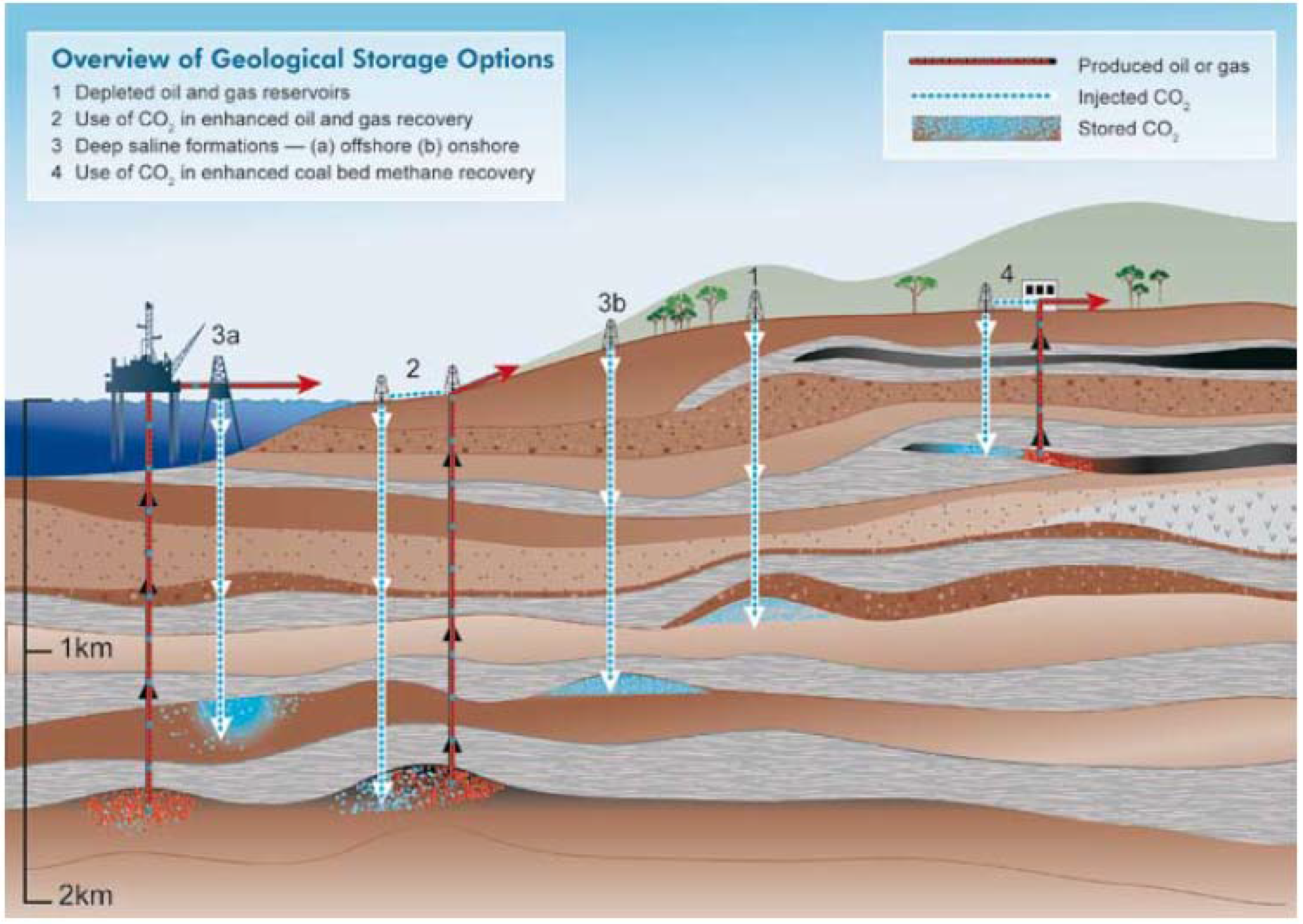
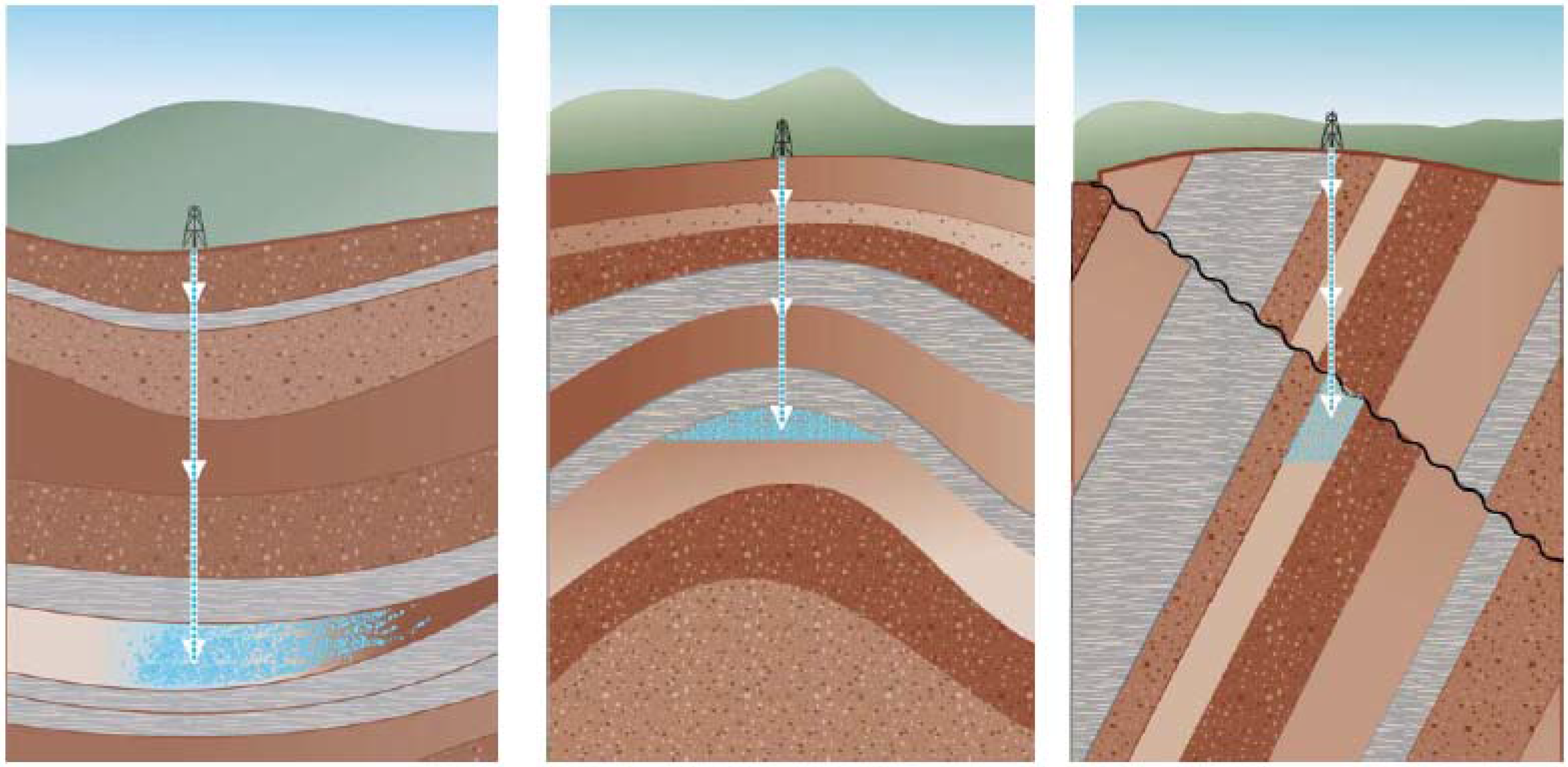
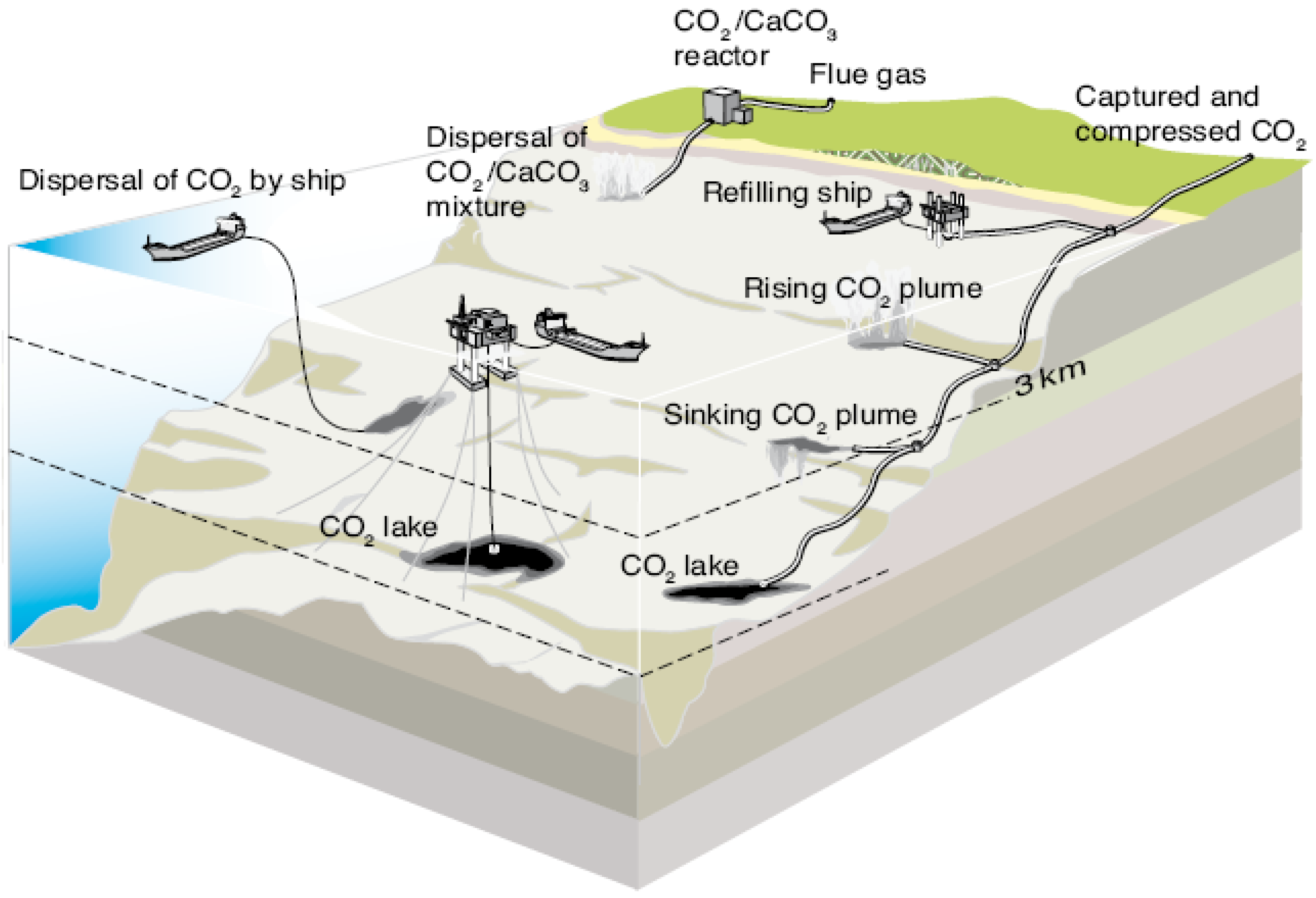
4.5. Geological Storage

4.5.1. Technical principle

Once separated, CO₂ is transported to a suitable storage site. Unless CO₂ quantities are small and distances large, this will most likely occur by high-pressure pipeline, a technology which has achieved maturity through extensive long-distance piping of CO₂, for example for enhanced oil recovery in Texas, USA [33]. CO₂ is then stored subterraneously through high-pressure injection at depths of more than 0.8 km, which is much deeper than usable sources of groundwater. The temperatures and pressures below this depth are above the critical values for CO₂ (31 °C and 72.8 atm; above the critical temperature, distinct liquid and gas phases of materials do not exist anymore. Instead, the gas and liquid phases gradually become the same as the critical temperature is reached, and eventually merge into a so-called supercritical fluid. From a supercritical fluid, no liquid but only a solid can be formed by increasing the pressure), to produce a supercritical fluid of 500 kg/m³ or denser [69]. This fluid diffuses through porous and permeable storage rock and occupies its intergranular spaces.

Figure 12. Geological storage options (after [33]).

Because it is less dense than water and oil (stored CO₂ densities are 50%–80% the density of water, and close to the density of stored crude oil) and hence buoyant, it must be trapped underground by impermeable cap rock above the injection point, just as natural gas, CO₂, and other gases have been trapped naturally for millions of years. This stratigraphic or structural trapping (Figure 13) is followed by dissolution and mineral trapping when CO₂ dissolved into underground saline water or oil, and even chemically reacts with the minerals of the surrounding rock, typically over hundreds of years. The injection pressure is chosen to be sufficiently high to force CO₂ into the porous space but low enough to not break through the cap rock. Suitable injection equipment is already widely used in the oil and gas industry. In the long term, suitable reservoirs are likely to be mostly deep saline aquifers, but can be depleted oil and gas fields. The distance of storage sites to earthquake faults matters, however a 6.8-Richter earthquake at 20 km distance from an injection site near Nagaoka in Japan did not lead to any detection of CO₂ leaks.

Another potential option is ocean storage, where CO₂ can form dense sinking plumes or bottom lakes when injected at depths of more than 3 km (Figure 14). Analysis of ocean currents suggest that injected CO₂ will be isolated for at least a few hundred years (Table TS.7 in [33]). However, the effects of increased CO₂ concentrations in ocean water on organisms, such as reduced calcification, are largely unknown. Further options are mineral carbonisation and industrial uses, but these options were considered less economical at the time of writing and shall therefore not be dealt with in detail.

Figure 13. Stratigraphic (left) and structural (middle and right) trapping (after [69]). © 2008 IEA/OECD, reproduced with permission from Geologic Storage of Carbon Dioxide - Staying Safely Underground, p. 7.

Figure 14. Methods of ocean storage of CO₂ (after [33]).

Calcination of CO₂ is described by Romeo et al. [92] as an emerging and potentially cost-effective method of capturing CO₂ off the flue gases into storage-ready form.

4.5.2. Capacity and load characteristics

The rate of CO₂ injection must be comparable to the rate of emission. Therefore, suitable storage rock must be able to distribute CO₂ rapidly enough from the injection point, or in other words, must have sufficient injectivity.

4.5.3. Life-cycle characteristics

The location of the storage site must be economically accessible to the emission source of CO₂, if possible without liquefaction, ship transport, or long-distance piping. However, even if ship transport is included, this will likely not represent more than 2% of the entire life-cycle emissions inventory [93]. Further details about life-cycle performance are given under the capture technologies.

4.5.4. Current scale of deployment

Routine CO₂ injection has been undertaken for more than three decades in the oil and gas industry (mainly Texas and New Mexico, USA) in order to enhance resource recovery (footnote 1 in [68], and page 2 of [69]). Current injection rates are in the order of 28 Mt CO₂/year [88]. Two storage and monitoring projects have injected so far more than 5 Mt CO₂ into a depleted oil field (Canada) and more than 10 Mt CO₂ into a deep saline formation (off-shore Norway) without detectable leakage [69]. More recent (2004) projects include a commercial natural gas recovery project in Algeria (1.2 Mt CO₂/ year), an enhanced gas recovery project in the Netherlands (8 Mt CO₂ / year), and an EU coal seam injection project (3 Mt CO₂/year). For further details see [88], and Table TS.5 in [33]. The IEA estimates a narrowing window of opportunity for CO₂-enhanced oil recovery to generate an additional 200 billion barrels of low-cost oil, equivalent to seven years of global production of 30–35 billion barrels per year [69]. Future applications will depend on mandating carbon capture and storage standards for power plants.

4.5.5. Contribution to global electricity supply

Using a spatial inventory of large point-emitters (above 0.1 Mt CO₂ per year) and comparing this to the global distribution of sedimentary basins, the IPCC (Table TS.6 in [33]) has estimated global storage capacity at about 200–2000 Gt CO₂, or equivalent to about 5–50 years of global emissions. However, the US reports storage capacity in saline aquifers and offshore oil and gas fields sufficient to hold 20–100 years of US emissions [88], and UK capacity is reported as equivalent to several centuries’ worth of current UK emissions [68]. A preliminary estimate by the IEA indicates that this may be the case globally [69].

4.5.6. Cost of electricity output

Assuming indicative aquifer storage cost of 10 US$/tCO₂, geological storage is estimated to add between 0.4 and 0.8 US¢/kWh to electricity cost including capture (p. 1173 in [82] and Table 1 in [68]).

2.1.1. Technical challenges

Rapid leakage paths for CO₂ exist for example in form of failed wells. Lower rates of seepage can be expected through known and unknown permeable faults, with the CO₂ driven either passively through diffusion, or through active porous flow facilitated by tidal pumping [94]. Estimates for leakage rates are rather low at less than 1% per thousand years [33], and thus low enough to not lead to long-term increases of atmospheric CO₂ concentrations [69]. Even at higher leakage rates, capture and storage would be able to make a meaningful contribution to climate change mitigation [33]. Understanding of leakage and movement of CO₂ is so far mainly obtained from complex numerical simulations, which constitutes one of the main uncertainties and barriers for the technology [67,71,72,73].

Future large-scale geological storage of CO₂ will benefit from advanced horizontal and directional drilling techniques, predictive modeling of underground displacement, migration and dispersion, seismic imaging for locating CO₂ underground, and continuous seepage monitoring [68].

The matching of the geographical distribution of large CO₂ point sources and suitable storage sites has to be assessed on a more detailed regional level. Major knowledge gaps exist for ocean storage and some other storage technologies. Other non-technical challenges include the need for legal and accounting frameworks, and for guidelines on leakage monitoring and prevention [95].

5. Nuclear Fission

5.1. Summary

Nuclear reactors currently operating are large (≈1000 MW) thermal-neutron reactors, operating at base load factors of around 85%. Nuclear power plants currently supply about 14% of the world’s electricity. They are in general are characterised by low operational (for example fuel) cost, but high upfront capital cost. These capital costs are largely responsible for the comparatively high investment risk requiring higher capital interest rates. According to Lim et al. [45] “electricity generation plants are typically financed by a combination of debt and equity. A ratio of 50%–50% or 60% debt to 40% equity is often used. The LCOE calculation must include the payments needed to service these debts. The amount of the interest payments depends on the interest rates assumed for each project. Since debt is senior to equity, the interest rate for debt financing is lower than the interest rate for equity financing. The weighted average cost of capital (WACC) is a common way to express the interest rates in a single number. […] The key driver behind choosing an interest rate is the risk that investors perceive for the project. High-risk projects require higher interest rates because investors need to be compensated for bearing the risk. […] Investors now have to internalize risks into investment decision making. This adds to the required rates of return and shortens the time frame that investors require to recover the capital. […] In many regions, nuclear power is perceived by investors as more risky than fossil-based power. This difference in perceived risk causes interest rates for nuclear projects to be greater than their fossil counterparts.” This applies especially “in countries or regions with deregulated or privatized energy markets, [where] the risk shield—[…] integrated monopolies can transfer costs and risks to ratepayers and taxpayers—has been partially or wholly dismantled” (see Figure 3–14 in [45]). Levelised electricity costs are sensitive towards these interest rates, but generally range between 3 and 7 US¢/kWh [45]. Life-cycle greenhouse gas emissions for current light water reactors are in the order of 65 g/kWh, but can vary depending on the grade of the uranium ore mined. Assuming 2007 reasonably assured and inferred resources of 5.5 MtU at < US$130/t [96], nuclear power could avoid at least 180 Gt CO₂ until 2100. The future of nuclear power appears to be strongly influenced by public perception and concerns about safety, waste disposal, and proliferation risk [13,14,65,97,98,99]. Further, at least in the US and much of Europe, the nuclear supply chain faces restrictions in form of skilled labour shortages and supplier market contractions, which may affect the quick re-activation of nuclear building programmes [2,32]. Finally, the indeterminate state of much spent fuel may lead to barriers for expansion in some countries [1]. These are some of the main reasons why nuclear electricity generation is projected by the IEA [64] (415–519 GW @ 2030) and the Energy Information Administration [100] (481 GW @ 2030; Figure 15) to increase at rates that are lower than overall electricity generation increase rates, except for China and India. In 2008, the OECD NEA issued its first own outlook [61], projecting in its high scenario a much steeper rise of nuclear capacity (600 GW @ 2030).

New Generation-IV reactor and fuel cycle technology holds promises for significant improvements regarding resource sustainability, inherent safety and sub-criticality, as well as substantial reductions in radioactive waste volumes and lifetimes, however these developments are not expected to be commercialized before 2030.

Figure 15. World nuclear electricity generation projections, in units of PWh (after [65]).

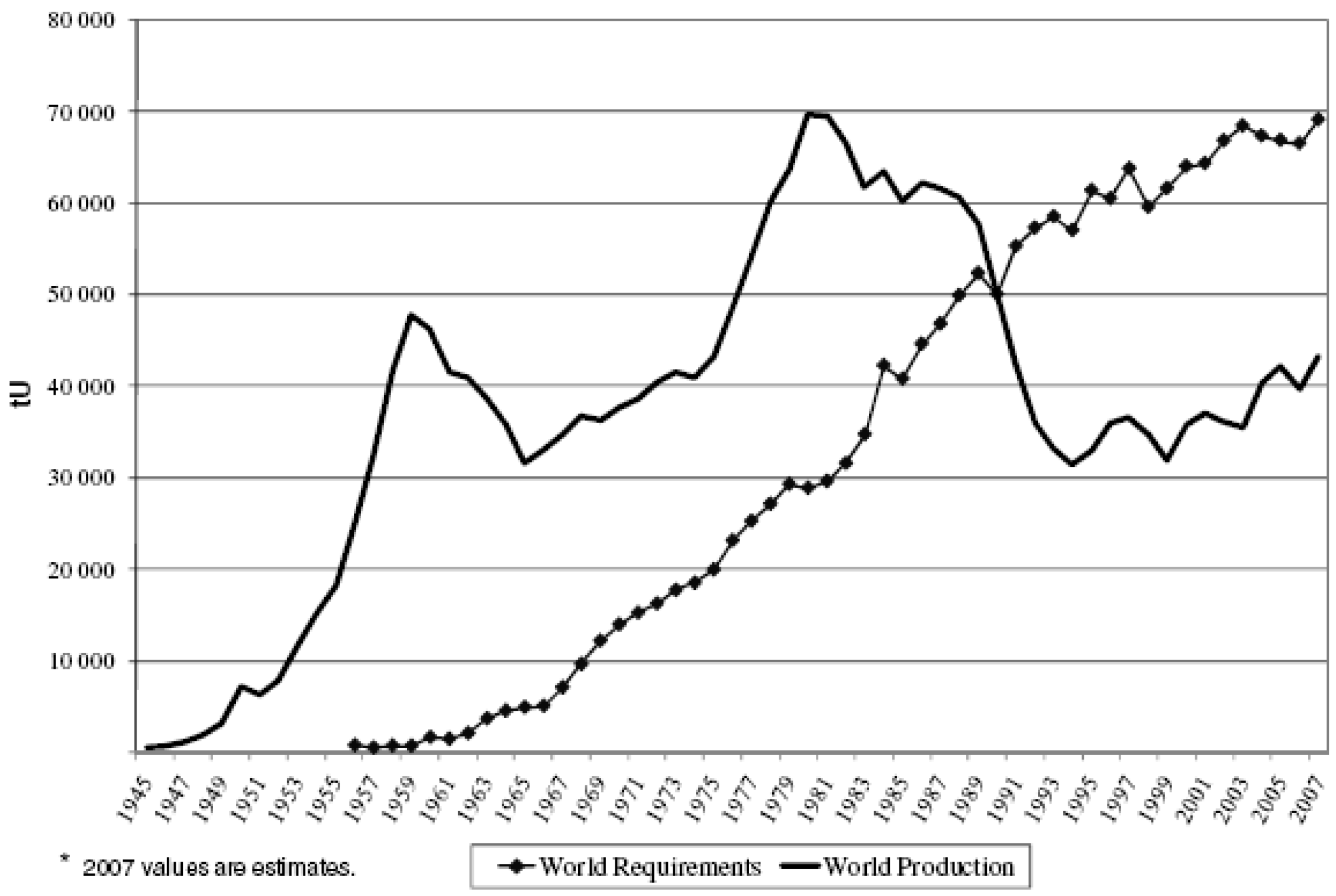
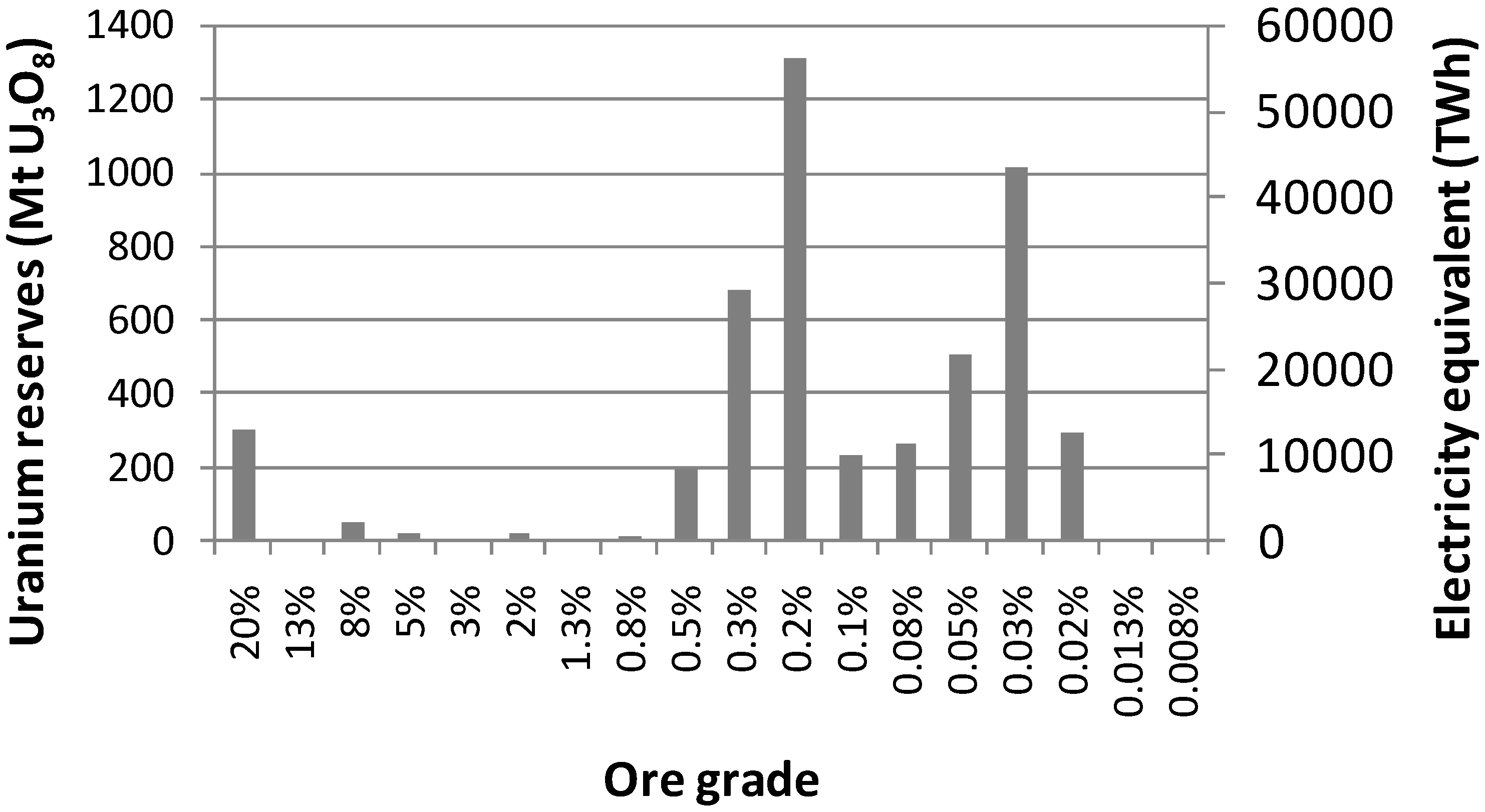
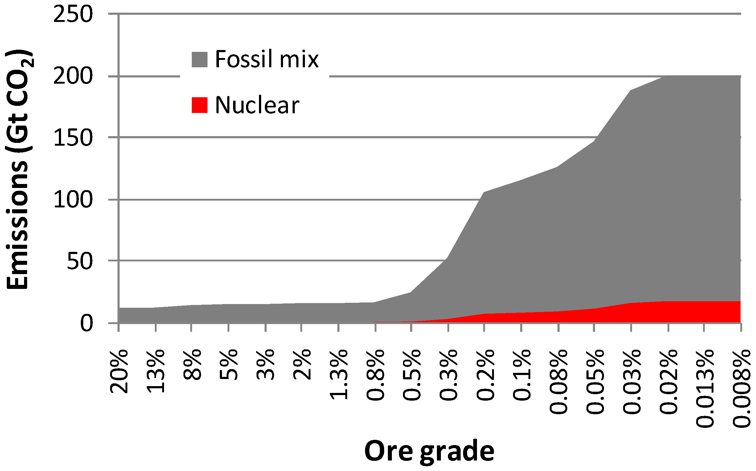
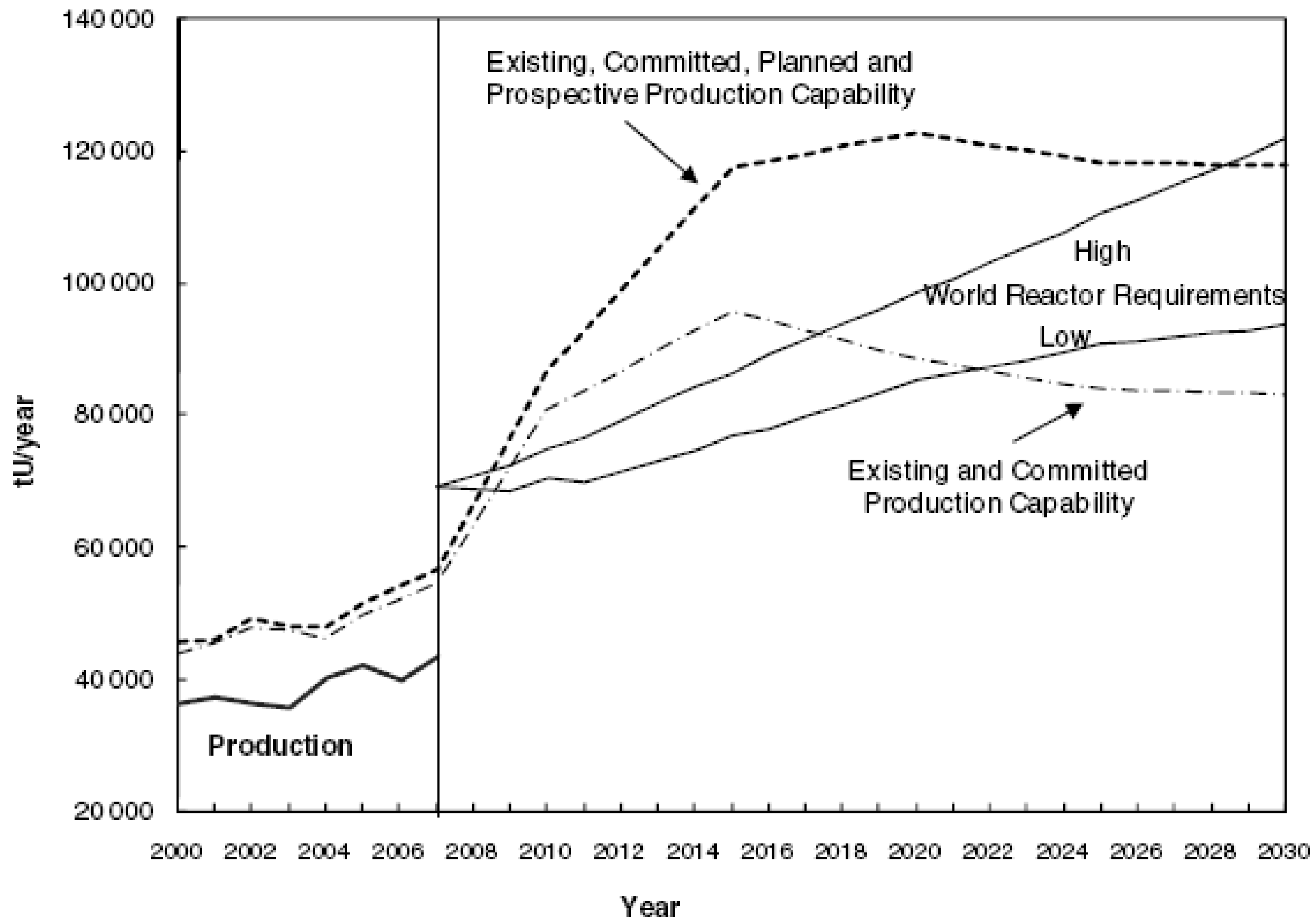
5.2. Global potential of resource

Between 1970 and about 1985, nuclear electricity production has experienced a rapid increase, however expansion slowed after the Chernobyl accident (Figure 16).

As long as there has been concern about climate change there has been a debate around the global potential of nuclear power. This debate focused on available uranium resources, but also on the life-cycle greenhouse gas emissions associated with recovering uranium from these reserves. Mortimer [101,102], Storm van Leeuwen and Smith [103] and Diesendorf [104] argued that with decreases in uranium ore grades the energy requirements would grow such that associated CO₂ emissions for mining uranium would become comparable to those of fossil-fuelled power plants. Mudd and Diesendorf [105] presents a detailed analysis of uranium mining.

Figure 16. Evolution of nuclear electricity production (TWh/year) by region. Asia excludes China, and “Other” includes Africa, Latin America and the Middle East. © 2008 OECD/IEA, reproduced from [17] with permission.

Little exploration for uranium was carried out in the 1980s and 1990s. The world’s demand for uranium has been to a significant extent (about 40%) met by relatively inexpensive secondary supplies such as canceled or shut-down reactors, stockpiles, or weapons ([32]; Figure 17), and production in recent years has been stable [96].

Uranium prices have increased since 2004 (Figure 18 and Figure 19), triggering new exploration activity (a 2½-fold increase of exploration expenditure overall between 2004 and 2006, and a 20-fold increase between 2002 and 2006 in Australia [96], Figure 20) and mine development, leading to continuing increase of resources (Figure 21; [106]).

Figure 21. Uranium exploration expenditure and RAR+inferred resources < US$80/t (from [107]). RAR+inferred resources < US$130/t are 5.5 MtU ([96]).

Figure 22. Uranium reserves [103,108]. Electricity equivalent calculated using 65 ktU/2,793 TWh ≈ 23 t/TWh.

In 2003, reasonably assured resources (RAR) and inferred resources were 3.2 MtU. Resources and production quantities are expressed in terms of tonnes (t) contained uranium (U) rather than uranium oxide (U₃O₈). 1 short ton U₃O₈ = 0.769 tU; 1% U3O8 = 0.848% U [96]. In 2005 these were 4.7 MtU, and in 2007 5.5 MtU ([96]; see also Figure 21). Throughout this section, NEA/IAEA definitions will be used. “Reasonably Assured Resources (RAR) refers to uranium that occurs in known mineral deposits of delineated size, grade and configuration such that the quantities which could be recovered within the given production cost ranges with currently proven mining and processing technology, can be specified. Estimates of tonnage and grade are based on specific sample data and measurements of the deposits and on knowledge of deposit characteristics. Reasonably Assured Resources have a high assurance of existence. Unless otherwise noted, RAR are expressed in terms of quantities of uranium recoverable from mineable ore (see Recoverable Resources).” “Inferred Resources refers to uranium, in addition to RAR, that is inferred to occur based on direct geological evidence, in extensions of well-explored deposits, or in deposits in which geological continuity has been established but where specific data, including measurements of the deposits, and knowledge of the deposit’s characteristics, are considered to be inadequate to classify the resource as RAR. Estimates of tonnage, grade and cost of further delineation and recovery are based on such sampling as is available and on knowledge of the deposit characteristics as determined in the best known parts of the deposit or in similar deposits. Less reliance can be placed on the estimates in this category than on those for RAR. Unless otherwise noted, Inferred Resources are expressed in terms of quantities of uranium recoverable from mineable ore (see Recoverable Resources).” See Figure A in [96] for a comparison of resource classifications.

RAR occur at ore grades between more than 20% and just above 0.01%; these have the potential to generate more than 200,000 TWh of electricity (see Figure 22). The greenhouse gas emissions resulting from the use of all RAR can be calculated by regressing results from the sensitivity analysis in [34]: Specific greenhouse gas intensities (e, in g/kWh) can be modeled as a function of ore grade (g, in %), yielding e = 26.8g^-0.16. Applying these greenhouse gas intensities to the electricity equivalent in Figure 23 yields emissions that would occur in uranium from ores of a certain grade were utilized for power generation. On a cumulative basis, starting with the richest ores, the nuclear fuel cycle would cause about 17 Gt CO₂ to be emitted for burning the entire RAR to generate 210,800 TWh of electricity (Figure 23). Generating the same amount of electricity using the 2006 fossil fuel mix would cause about 198 Gt CO₂ to be emitted. Exhausting all RAR would hence avoid about 180 Gt CO₂. This agrees with previous estimates by Pasztor [97] and Donaldson and Betteridge [109]. Tokimatsu et al. [110] carry out a dynamic study for Japan, and show that over a period of 65 years, LWR avoid about 25 Gt compared to a phase-out scenario.

Figure 23. Cumulative greenhouse gas emissions associated with the generation of the electricity equivalent in Figure 17, from ores with decreasing ore grades, using nuclear power plants (red), and as an alternative the 2006 mix of coal (61%), oil (9%) and gas (30%) plants (grey).

2007 RAR and inferred resources would provide electricity for about 85 years at current generation rates (compare [107]). This estimate decreases somewhat if an increase of current nuclear generation is assumed (compare [111]), however, uranium resources are likely to last longer than one life time of a reactor, which means that even under a nuclear expansion program, reactors would not have to be decommissioned early. Including improvements in reactor efficiency, reprocessing of spent fuel, and utilisation of 600 kt weapons-grade Highly-Enriched Uranium (HEU; [112]), 2007 RAR and inferred resources would last longer than 100 years at current production rates [113]. This does not take into account that significant increase in exploration effort could readily double the known economic resources [107]. However, the grade of future discoveries is unknown. The OECD Red Book does not provide data on the grades of ore mined over time but data in [105] indicate that recent discoveries have been of lower grade than earlier discoveries, with the possible exception of Canada.

The ultimately resource potential of nuclear fuels depends also critically on whether breeder fuel cycles are employed or not (see Section 5.4.1.1). Whilst currently only less than 1% of the nuclear energy in the uranium is exploited, breeding could raise this to 50% and above, stretching the lifetime of resources to many hundreds of years. However, breeder fuel cycles are the subject of controversy because of their associated cost, safety and proliferation risk, and the operational record of existing breeder reactors [102,104,114].

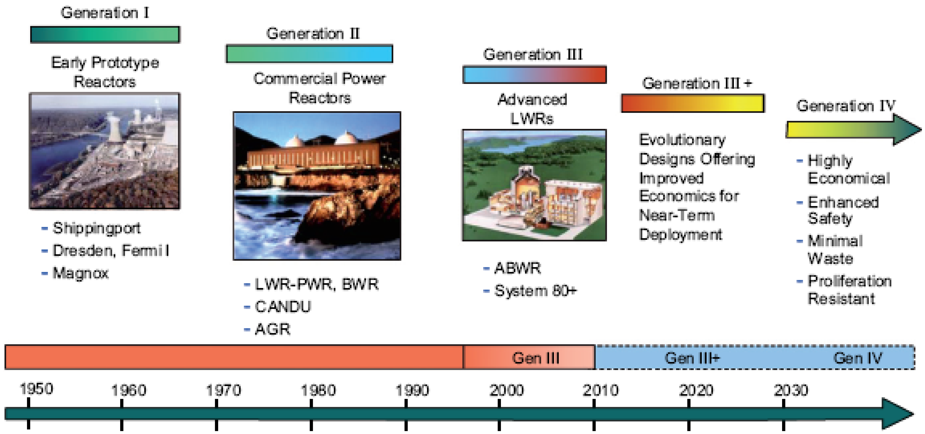
5.3. Generation-II and -III reactors

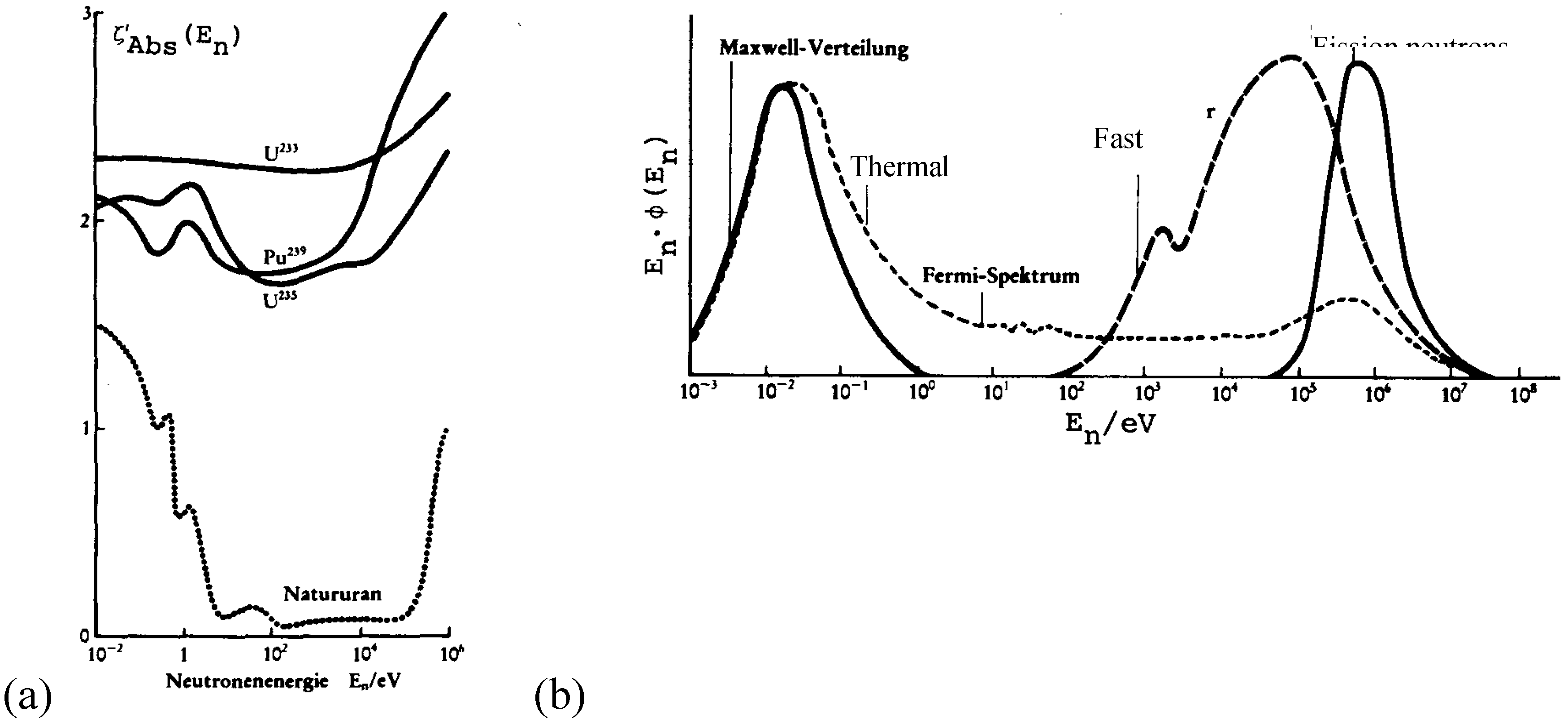
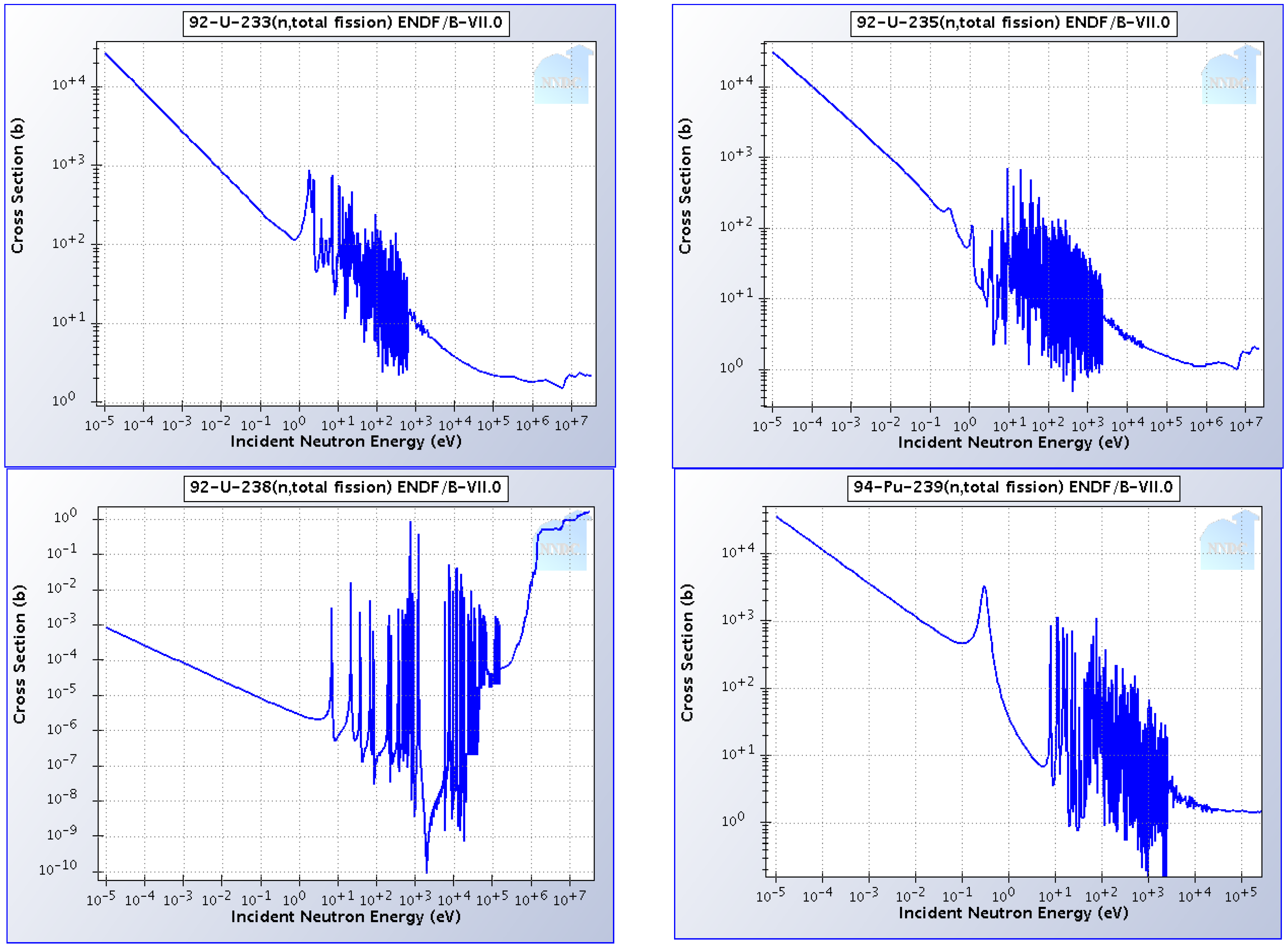
5.3.1. Technical principle

Nuclear power plants exploit the energy that is bound in heavy atomic nuclei and that gets released when those nuclei undergo fission. Nuclear fission can be achieved in a nuclear reactor by colliding heavy nuclei (U-235, Pu-239, U-233) with neutrons. During the fission the nuclear energy is converted into kinetic energy of the fission products, which in turn is converted into reactor coolant heat. Fission products are principally two light nuclei, gamma radiation and fission neutrons. The latter are available for triggering new fission events, thus enabling a chain reaction. This chain reaction can be controlled by neutron-absorbing substances, such as so-called neutron poisons that are either fission products building up during reactor operation, or effective neutron absorbers deliberately placed in control rods. Heavy nuclei have their own characteristics with regard to fission and neutron absorption probabilities, usually referred to as cross-sections. Fission-cross sections, as well as ratios of fission and caption cross sections, vary substantially for slow and fast neutrons (Table 2).

Fission-generated neutrons are fast neutrons, so if U-235 is to be used in a conventional nuclear reactor (that is not a fast breeder), these neutrons have to be slowed down in order to trigger new fission events. This slowing down is achieved by a neutron moderator. The heat generated in the reactor core is carried away by the coolant (often water, but also helium, and liquid metals) and used to generate steam which in turn drives a turbine. In Pressurised Water Reactors (PWR), the water coolant cycle is physically separate from the turbine cycle, whilst in Boiling Water Reactors (BWR) the coolant is made to boil in the reactor core and directly drives the turbine.

Table 2. Fission (σ_f) and caption (σ_c) cross-sections and their ratios α = σ_c / σ_f for a range of isotopes, and in two neutron energy ranges. The smaller α, the higher the probability for neutrons to cause fission. U-235 neutron caption is more likely to lead to fission for slow neutrons (PWR spectrum), whilst for Pu-239 this is the case for fast neutrons. Another important characteristic (not listed here) is the relative importance of the absorption cross-section of non-fissile isotopes such as U-238. © 2002 Elsevier, reproduced with permission from [115].

**Table 2.** Fission (σ_f) and caption (σ_c) cross-sections and their ratios α = σ_c / σ_f for a range of isotopes, and in two neutron energy ranges. The smaller α, the higher the probability for neutrons to cause fission. U-235 neutron caption is more likely to lead to fission for slow neutrons (PWR spectrum), whilst for Pu-239 this is the case for fast neutrons. Another important characteristic (not listed here) is the relative importance of the absorption cross-section of non-fissile isotopes such as U-238. © 2002 Elsevier, reproduced with permission from [115].

In some reactor types, the coolant and the moderator are one and the same medium, which provides a certain degree of passive safety (see Section 4.4.1.5). Commonly used moderators include regular (light) water (75% of the world’s reactors; PWR and BWR), solid graphite (20%; gas-cooled GCR) and heavy water (5%; HWR). The energy density of uranium is in the order of a million times larger than that of coal. Therefore, even large nuclear reactors need only about 30 tonnes of uranium to operate a whole year.

5.3.2. Capacity and load characteristics

Nuclear power is a base load technology. In 2006, 2793 TWh of nuclear electricity were generated with 370 GW installed capacity, yielding a load factor of 86% [17]. Most of the world’s capacity resides in the United States (99 GW), followed by France (63 GW), Japan (48 GW), Russia (22 GW), Germany (20 GW), South Korea (17 GW), Ukraine and Canada (both 13 GW), the UK (10 GW), and Sweden (9 GW). Recent US load factors have exceeded 90%, as reported by Lim et al. [45] (Figure 3-17) and Blake [42].

5.3.3. Life-cycle characteristics

Life-cycle greenhouse gas emissions came to the fore of energy futures debate along with renewed suggestions that nuclear power could play a vital role in mitigating climate change. For example Mortimer [101,102] highlights incorrect claims for nuclear energy being a carbon-free energy source.

In a comprehensive survey of life-cycles studies of nuclear power, Lenzen [34] establishes a range of life-cycle greenhouse gas emissions of 10–130 g/kWh. This range was confirmed in slightly updated studies by Fthenakis and Kim [116] and Sovacool [44]. A multiple regression of 52 literature studies, and a sensitivity analysis in [34] yielded that—as expected—the life-cycle energy performance of nuclear power plants is mainly influenced by ore grades, enrichment technology, and by re-load frequency and burn-up, and to a lesser extent by enrichment level, plant lifetime, load factors, and enrichment tails assay. Future trends in enrichment technology, ore grades etc are hence going to influence emissions.

Storm van Leeuwen and Smith [103] arrived at significantly higher values, which for low ore grades placed nuclear power into the vicinity of advanced natural gas plants. As Lenzen et al. [47] showed, this discrepancy is mainly the result of practices assumed by Storm van Leeuwen and Smith [103] (but not applied currently, see p. 18 in [117]) for the final disposal of large volumes of low-level ore, waste rock, and mill tailings. The worst case in [47]—0.01% ore grade, 75% load factor, 25 year lifetime, only diffusion enrichment, and a carbon-intensive background economy (compare with results in [29] and [30])—resulted in emissions of 248 g/kWh, which also agrees with the maximum value found by Sovacool [44], but still below the estimate that can be derived from [103]. The issue surrounding the energy requirement for mine clean-up is essentially dependent on judgments of what constitutes sufficiently safe practices with regard to minimizing radioactivity from Radon, as well as toxicity from heavy metals in low-level ore, waste rock, and mill tailings [118]. It is therefore necessary to describe the main sources of radiological exposure from uranium mining. At the time of extraction of the uranium from the ore, about 85% of the original radioactivity remains in the mill tailings in form of long-lived uranium daughters, notably Th-230 and Ra-226 that were in equilibrium with the U-235 and U-238 isotopes (Figure 24).

Of those, Th-230 has the dominant half life of about 75,000 years. Alpha decay of Ra-226 produces 222-Rn (“Radon”), which as a noble gas emanates into the air adjacent to the tailings, and represents the main radiological concern not only from uranium mining operations, but in fact from the entire nuclear fuel chain [118]. When inhaled, Radon can decay into its daughter Po-218 (“Polonium”), which as an ion can attach itself to human lung tissue, and, at sufficiently high exposure, can cause elevated lung cancer risk [119]. Radon occurs naturally, and is responsible for an average radiation dose to humans of about 1–2 mSv/y, depending on location [120] (the Sievert (Sv), or milliSievert (mSv), is the unit of the so-called dose equivalent, which measures the effective biological impact from exposure, weighted by type of radiation (alpha, beta, gamma), by organ types, and other factors [119]).

Mudd [119,122] has compiled a large and detailed body of information available on radioactivity releases from operating and closed uranium mines. Whilst there is agreement that emissions and safety standards have vastly improved since the 1950s, there are conflicting conclusions about the level of safety provided by current practices, and the success or failure of current mine rehabilitation efforts [121,123,124,125,126].

According to the United Nations Scientific Committee on the Effects of Atomic Radiation (UNSCEAR), the global component from mill tailings is the most significant source of radiological exposure in the entire nuclear fuel chain. This holds irrespective of whether the 1993 or 2000 assessment is taken as a basis (Table 1 in [122]). Taking the higher estimate as morerealistic [127], 150 Sv/GW_e translate into 55.5 kSv globally, which is equivalent to an annual dose of about 0.01 mSv/capita if the entire world population were equally exposed. This estimate agrees well with ranges given in the assessment of uranium mines by Nilsson and Randhem [128], who state a range of 0.1 to 0.001 mSv/cap.

The local and regional component of exposure from mining is smaller, but it applies to a smaller number of people. The World Nuclear Association [120] has published average (1.5–2 mSv/y) and maximum doses (10 mSv/y) to Australian uranium miners. These estimates are confirmed in [128]. The maximum doses are five to ten times higher than natural background doses from Radon, but also five times smaller than doses received by people living in locations with high concentrations of radioactive elements in natural soils and rocks (for example Kerala, India, and Minas Gerais, Brazil), where no elevated lung cancer incidences could be detected [129].

In summary, the major component of radiological exposure from the nuclear fuel cycle is the global component from mill tailings, distributed around 0.01 mSv/cap annually. The local component is about 100 times smaller, but larger per capita at about 2 mSv/cap annually. These compare to background radiation from Radon in the order of 1–2 mSv/cap annually. On the basis of available measurements it appears that current mine rehabilitation does not lead to radiological exposures that would explain changes in practice proposed by Storm van Leeuwen and Smith [103] to the extent that these changes would lead to greenhouse gas emissions that are twice the amount of those for mining.

Wider adoption of in-situ leach mining [130] may alleviate the implications for nuclear power of Radon emissions from mine tailings, and low-grade ore and waste rock piles, as well as energy requirements of mine clean-up. However in-situ practices are still under development, and bring with them their own issues regarding groundwater pollution [131,132].

5.3.4. Current scale of deployment

The typical scale of reactor deployment is in the order of 1,000 MW. More than half of the world’s reactors are of the PWR type, 94 BWR, 44 Heavy Water Reactors, 16 graphite-moderated reactors, 18 gas-cooled reactors, and two fast breeders (Table A5.1 in [61]).

5.3.5. Contribution to global electricity supply

Electricity from nuclear fission grew from 203 TWh in 1973 to 2793 TWh in 2006 [17]. More than 80% of nuclear power generation occurs in OECD countries (29% United States, 16% France, 11% Japan, 6% Germany, 5.5% Russia, 5% South Korea, 3.5% Canada, 3% UK, 2.5% Sweden; all figures rounded [17]), about 9% in the Former Soviet Union, and 2% each in China and non-OECD Asia.

In 2006, 435 nuclear power plants operating in 30 countries provided 14.8% of the world’s electricity [17]. Regional shares vary widely, with France leading at 79%, followed by Sweden and Ukraine (both 46.7%), South Korea (37%), Japan (27.8%), Germany (26.6%), the UK and USA (both 19.1%), Canada (16%), and Russia (15.7%).

Whilst short-term barriers for the deployment of fast reactors are posed by discoveries of readily accessible uranium reserves [133], the literature shows that the barriers for large-scale and long-term deployment of nuclear power are mostly cost, but rather to perceived operating safety, waste disposal issues, and proliferation risk, with implications for financial risk and interest rates ([63,134], and Section 3.3 in [55]). This has not changed during the past two decades (compare with [97] and [135]). The literature stresses that especially the safety of long-term waste disposal is hard to prove, given the very long time horizons, and the lack of experience. Further, in the public perception, nuclear energy is often perceived as an invisible danger under the control of a few, and associated with military use, suppression of information, and high accident risk [13,14,97,98]. Whether scientifically founded or not ([12], p. 17, states that “the proponents of a ‘technical’ approach to risk management have long considered that the public’s perceptions were unfounded and should not interfere with the objective assessment of risks. At the same time it is increasingly accepted that although the public perception of risk can be wrong (for instance if it is distorted by orchestrated campaigns by vested interests), there is no objective and unique measure of risk. Risk has a multitude of dimensions, some of which involve ethical considerations. A number of different views can thus be pertinent and legitimate, and confronting this variety of standpoints is part of risk management.”), this perception cannot be brushed aside: public acceptance of nuclear energy has become as much an issue of technology as of philosophy and lifestyles. This is reflected for example in the vastly different histories of spent nuclear fuel (currently about 270,000 tonnes, with 10,000–12,000 tonnes added each year, and 3,000 being reprocessed [136]) policies across different countries: whilst the German anti-nuclear movement has achieved a stagnation in spent-fuel policy-making, the greater pragmatism of the discussion in Finland has led to the Green Party supporting the final disposal option, and only small amounts of protest in Japan (despite Japan’s WWII history, but perhaps in the context of a dense population and unstable geology making final disposal highly unattractive) have allowed for the reprocessing option [13]. Views of what constitutes sustainable development has also led to nuclear power being excluded from two of the three flexibility mechanisms in the Kyoto Protocol. Whilst this exclusion is largely symbolic in terms of pre-2012 capacity development, it does reflect decision-makers’ attitudes towards nuclear power, and the need for the nuclear industry to provide complete, unbiased and reliable information [61,99]. The inclusion of nuclear power into the Kyoto mechanisms (Clean Development Mechanism, CDM, and Joint Implementation, JI) was on the agenda of the Copenhagen Conference scheduled for December 2009. A survey in the EC yielded that scientists and non-governmental organisations (NGOs) are the most trusted groups to provide such information [61,99]. However, often these two groups may also hold the most opposing views.

Fast-breeder technology provides solutions for the waste issue, but cannot yet satisfactorily deal with operating safety and proliferation concerns (see Table 3). This is reflected in only six out of 32 countries that possess nuclear technologies allowing the reprocessing of spent nuclear fuel [13]. On the other hand, R&D efforts on nuclear technologies have increased in recent years [137,138]. Safety, sustainability, disposal and proliferation issues, or high prices of uranium may provide incentives for the development of advanced systems, for example dedicated transmuters using accelerator-driven sub-critical reactors, and thorium-based fuel cycles [139], or flexible systems that can provide hydrogen and high-temperature heat in addition to electricity [138].

5.3.6. Cost of electricity output

In contrast to gas-fuelled power plants, and to a lesser extent also coal-fuelled power plants, fuel costs are a minor component for nuclear generating cost, though upfront capital costs are considerably higher [140]. Nuclear reactors can store fuel on-site for many years of operation [63]. This is why nuclear electricity is less affected by resource price volatility, but more by investment conditions such as interest rates and government regulation [2].

A report by the US Electric Power Research Institute (EPRI) commissioned for the Australian Uranium Mining, Processing and Nuclear Energy Review (UMPNER) provides a comparative review of recent studies of levelised cost of nuclear electricity [45]. Levelised costs are defined as the constant (discounted to present values) real wholesale price of electricity that recoups owners’ and investors’ capital costs, operating costs, fuel costs, income taxes, and associated cash flow constraints. They exclude costs for transmission and distribution. In other words, levelised costs are plant boundary cost [31,45]. Levelised cost may differ prom sales prices, because of profits or losses. EPRI lists results from six studies (their Figure ES-1) showing that in the US nuclear power was more expensive than coal- and gas-fuelled power, about equally expensive in the UK, and less expensive in Australia and Finland. Lim et al. [45] explain the reasons for the diverging results. First and clearly, assumed interest rates for invested capital play a large role in electricity cost, since nuclear power has longer lead- and life-times and is more capital-intensive upfront than coal- and gas-based technologies. This means that in a deregulated economic environment where private investors have to finance capacity developments, the perceived financial risk is higher and therefore requires higher premium, that is, interest rates on capital, thus leading to higher cost (the terms “regulated” and “deregulated” are used in standard ways to describe a transition from a government-owned industry to a competitive market setting. In the latter, the risk has to be borne by investors and cannot be passed on to taxpayers, hence the interest rate discussion). This is confirmed in a study by the OECD NEA and IEA [31], where nuclear is the least expensive option at 5% interest rate, but overlaps with coal and gas technologies at 10% interest rate. After converting cost estimates from all studies to one base year and currency, Lim et al. [45] (Figure 25) were able to demonstrate that interest rates influence nuclear generating cost more than they influence those of coal and gas, and that cost from all studies and technologies converged at about 4–5 US¢/kWh for an interest rates between 6% and 7%. Increases in interest rates was also attributed as an important factor leading to cost escalations in the 1980s [141]. Second, some studies indicated that learning-by-doing influenced long-term cost. This was shown to be especially the case in Australia, where nuclear engineering and operating skills are lacking at present. Third, competitiveness also depends on the prices of coal and gas, which were—at least at the time of Lim et al.’s writing—more volatile than those of uranium. Fourth, standardized regulatory procedures such as combined construction and operation licences, and design certification, are expected to be major prerequisites for low construction cost [135]. According to Lim et al. [45], decommissioning and spent fuel and waste disposal is not expected to add significantly to levelised cost. Estimates are in the range of 0.1–0.2 US¢/kWh [136] but, given the most recent US Department of Energy estimates for the Yucca Mountain facility, could be as high as 0.5 US¢/kWh. However, uncertainty about these estimates exists because they are largely based on ex-ante waste fees, and not on operational long-term repository (Lim et al. [45] report that “owners also accumulate funds for eventual decommissioning and dismantling of the plant, as well as for spent fuel disposal, by assessing consumers a small additional charge. […] In the United States, the federal government has levied a standard nuclear waste fee of 0.1 cent/kWh generated by nuclear plants. […].”). It seems however clear that at least for Uranium prices below US$ 300/kgU, geological disposal is less expensive than reprocessing for either thermal-neutron light-water reactors, fast-neutron reactors, or future transmutation facilities [142].

Another clear finding from [45] is that the internalisation of external cost into fossil-fuelled power generation, for example by imposing carbon taxes, would radically alter the competitive landscape in favour of nuclear power, because additional cost for carbon capture are in the order of, or higher than the cost gap between nuclear and fossil power. Whilst nuclear electricity ranges between 4 and 7 US¢/kWh, fossil power without capture is generally less expensive than nuclear at 3–6 US¢/kWh, but can be more expensive at 5–9 US¢/kWh if capture is included (compare with page 6 in [143]).

These findings are confirmed in a US study by Harding [32] who takes into account major commodity price hikes, and the re-evaluation of older long-term fuel contracts based on current uranium spot prices. Using peak yellowcake prices of US$135/lbU₃O₈, nuclear electricity ranges between 9 and 10 US¢/kWh, whilst fossil power without capture is generally less expensive than nuclear at 6–7 US¢/kWh, but can be more expensive at 10–12 US¢/kWh if capture is included. Harding notes that fossil power plant operators may opt for carbon credits, because if these cost US$30 per metric tonne of CO₂, or about 1.5–3 US¢/kWh, they would be less expensive than carbon capture technology installation. Harding also quotes cost data from recently (post-2002) built plants in Japan and South Korea, which clearly demonstrates that low labour rates can cut overnight and O&M cost, and to some degree also levelised electricity cost, by up to 40%. A bottom-up study of learning curves by Neij [144] indicates stabilization of levelised cost.

5.3.7. Technical challenges

All LWR have the disadvantage in that they are not very efficient in exploiting the natural resource in their fuel. At conversion ratios around 0.55 in a once-through cycle only 0.5% of the primary nuclear energy is converted into useful heat. Even recycling spent fuel into mixed-oxide (MOX) fuel exploits only about 1% (see Figure 26). This means that LWR show poor energy resource sustainability.

Most nuclear reactors operated today must be engineered for safety with multiple safety systems and costly containment measures. Further, there is a lack of technical experience with technologies for final geological disposal of long-lived radioactive waste [61,99], and with safe international reprocessing routes, leading to most countries opting at present for interim storage, pending further policy development [13]. These issues are further elaborated on in Section 4.4.7.

Harding [32] described technical challenges related to restrictions in the supply chains of nuclear reactor operations, such as enrichment capacity, skilled labour, experienced contractors, and major supply parts such as pressure vessels. These restrictions are the result of consolidation and retrenchment in the nuclear industry during the low-demand period of the 1980s and 1990s. High market concentration leading to reduced supply flexibility is a concern especially in front-end stages such as fuel conversion, enrichment and fabrication [146,147]. Harding argues that with many reactors being decommissioned within the following two decades (see Figure 27 and Figure 28), and not many having been built over the past decade (less than 0.5 GW per year since 1996, see Figure 26), crucial technical experience for the maintenance, let alone significant expansion, of nuclear construction and operation programs may be lacking (compare [2]). He concludes that mining and enrichment capacity must be doubled over the next few years just to meet current demand for nuclear electricity, especially since secondary uranium sources are projected to decline by 2013 [96]. The requirements for growth scenarios such as in [64], [65] and [61]—amounting to newly installed capacity between 2 and 6 GW per year (Harding notes that such growth rates have been sustained in the past, however under different circumstances, that is, with significantly larger supplier and labour bases) (Table 4 in [32]) or more ([61])—would be higher, placing more demands on the timely availability of key personnel and reactor components, and on financial contracts that keep investor risk at an acceptable level. This view is confirmed in the OECD NEA and IAEA Red Book [96] (“despite the significant additions to production capability reported here, there remains pressure to bring facilities into production in a timely fashion. To do so, strong market conditions will be required to bring the necessary investment to the industry”, Figure 29).

5.4. Generation-IV reactors

Generation-IV reactors are currently being designed and researched under the umbrella of the Generation-IV International Forum (GIF; http://www.gen-4.org/), based on eight technology goals. The primary goals are to

improve nuclear safety,
improve proliferation resistance,
minimise waste and
natural resource sustainability,

and to decrease the cost to build and run such plants. The following table provides a summary assessment.

Table 3. Summary criteria for advanced nuclear systems.

**Table 3.** Summary criteria for advanced nuclear systems.
Type	passive safety	resource sustainability	waste minimisation	proliferation resistance	competitive power	Comments
Gen III+ LWR	✓			✓	✓
FBR		✓	✓		✓
MSR	✓			✓	✓	Can use on-site reprocessing
MPBR	✓			✓	✓	Spent fuel can be transmuted ^a
ADS	✓	✓	✓	✓^b		Minor contribution to power generation

Acronyms: LWR – Light Water Reactor; FBR – Fast Breeder Reactor; MSR – Molten Salt Reactor; MPBR – Modular Pebble Bed Reactor; ADS – Accelerator-Driven System; ^a [148]; ^b if Pu is considered as waste.

An often expressed strategy that would enable resource sustainability and waste minimisation whilst operating all plants at a high safety level (i.e., without using fast critical reactors) is the deployment of advanced (Gen III+) LWR as burner plants in conjunction with sub-critical ADS plants dedicated for breeding and waste transmutation [145]. This strategy is an effective alternative to the use of breeder reactors, in that it utilizes in excess of 50% of the natural uranium resource.

5.4.1. Technical principle

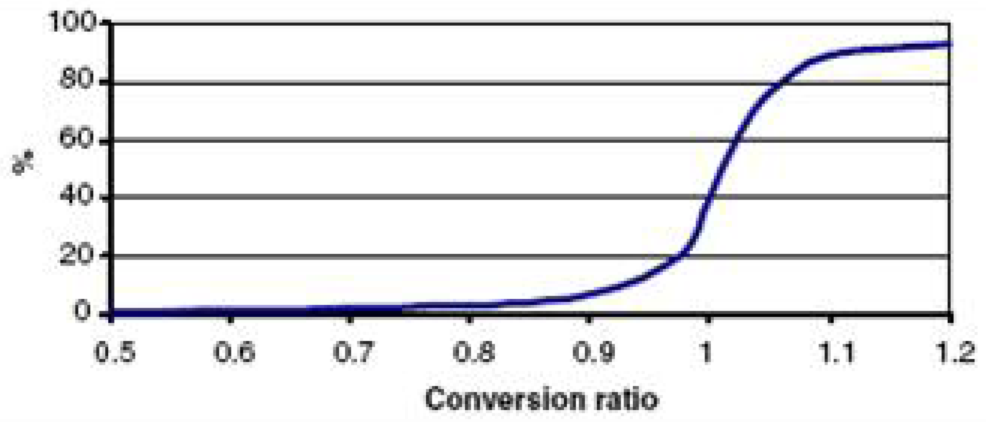
The reactor types chosen for priority investigation are (www.gen-4.org; [149]; Table 4) the gas-cooled fast reactor (GFR), lead-cooled fast reactor (LFR), molten-salt reactor (MSR), sodium-cooled fast reactor (SFR), supercritical water reactor (SCWR), and the very high temperature reactor (VHTR). In addition to the broad classification listed above, there is a wealth of pursued technology options such as thorium cycles, partitioning and transmutation. These technologies can all be employed in conjunction, making up a large array of nuclear fuel strategies. Therefore in the following, a brief overview over the main technological concepts for advanced nuclear power is provided.

5.4.1.1. Breeding

Fertile U-238 can be converted into fissile Pu-239 through capturing a neutron, thus “breeding” new fuel. In a breeder reactor more new fuel is generated than existing fuel consumed. These systems have conversion ratios above 1, and hence make better use of the nuclear energy contained in the natural resource (Figure 25). Breeder reactors were first considered in the 1970s for improving energy security and energy sustainability. Today the interest in breeder reactors exists more because of their ability to reduce volumes of long-lived nuclear waste. Breeder reactors can utilize the uranium (U-238-Pu-239) as well as the thorium cycle (Th-232-U-233). In practice, all proposed breeder reactor programs involve reprocessing of the fuel.

**Table 4.** Overview of Gen-IV reactor characteristics [133]. © 2008 Elsevier, reproduced with permission.
System	Abbreviation	Neutron Spectrum	Coolant	Maximum Temperature (°C)	Pressure	Fuel	Fuel Cycle	Output (MW_e)	Output
Gas-cooled fast reactor	GFR	Fast	Helium	850	High	U-238, MOX	In situ closed	288	Electricity, hydrogen production
Liquid metal (e.g., Pb) cooled fast reactor	LMFR	Fast	Pb-Bi	550–800	Low	U-238, MOX	Closed, regional	50–150, 300–400, 1200	Electricity, hydrogen production
Molten-salt reactor	MSR	Epithermal	Floride salts	700–800	Low	UF₆ in salt	In situ closed	1000	Electricity, hydrogen production
Sodium-cooled fast reactor	SFR	Fast	Sodium	550	Low	U-238, MOX	Closed	300–1500	Electricity
Supercritical, water-cooled reactor	SCWR	Thermal; fast	Water	510–550	Very high	UO₂	Open (th), closed (f)	1500	Electricity
Very high-temperature gas-cooled reactor (as in the GA system)	VHTR	Thermal	Helium	1000	High	UO₂	Open	250	Electricity, hydrogen production

5.4.1.2. Fast reactors

On average, fissions caused by fast neutrons produce more neutrons than fissions caused by thermal neutrons (most neutrons emitted by fission events are prompt: they are emitted essentially instantaneously. Once emitted, the average neutron lifetime in a typical core is on the order of a millisecond. Nuclear weapons are engineered to maximize the power growth rate, and so rely on prompt neutrons with lifetimes well under a millisecond) (Figure 30).

Therefore, in a fast reactor, there is a much larger excess of neutrons not required to sustain the chain reaction. On the other hand, fast reactors are more difficult to control first because they require special engineering (instead of a moderator) to ensure negative coefficients of thermal reactivity, and second because regulating their criticality relies solely on a fraction of fast fission neutrons that are delayed (about 15 seconds on average). The average life time of prompt and delayed neutrons together is increased (to about 0.1 seconds) through the presence of these delayed neutrons, so that the reactor is controllable. Fast reactors are operated in a prompt subcritical, delayed critical condition: the prompt neutrons alone cannot sustain a chain reaction, but the delayed neutrons make up the small difference required to produce as many new neutrons as become captured. A fast reactor does not need any neutron moderator, but its fuel must be more highly enriched than the fuel in a thermal reactor, because the Pu-239 fission cross-section is much lower for fast neutrons than it is for thermal neutrons (see Figure 31).

Figure 30. (a) Energy spectrum of thermal, fast and fission neutrons. (b) Neutron yield (y-axis as a function of neutron energy (x-axis). The faster the incident neutrons, the more fission neutrons are obtained from fission. Natururan = natural uranium (after [150]). © 1984 Oldenbourg Verlag, reproduced with permission from [150].

Figure 31. Fission cross sections for U-233, U-235, U-238 and Pu-239. U-233, U-235 and Pu-239 have high fission cross-sections for thermal neutrons and low fission cross–sections for fast neutrons. The opposite is true for U-238. Retrieved from National Nuclear Data Centre (www.nndc.bnl.gov/sigma).

Fast reactors produce enough excess neutrons to breed more fuel than they consume (see Section 5.4.1.3). Fast neutrons also enable the transmutation of nuclear waste, because the fission cross-sections of plutonium and minor actinides are much higher than their absorption cross-sections in a fast spectrum (Table 1 in [115]). A fast reactor can be operated as a breeder or as a burner, depending on the need at the time. The coolant in a fast breeder reactor may not be a neutron moderator, therefore liquid metals, supercritical water, or gases are used instead of water. Generation-IV proposals include gas- and liquid-metal-cooled designs. Liquid metals (sodium and lead) have been chosen as fast reactor coolants historically because of their excellent heat transfer properties and low neutron interactions, and also because they enable a very compact design.

5.4.1.3. Fast and thermal breeder reactors

A fast reactor has sufficient excess neutrons so it can not only sustain a chain reaction but also convert, or breed, fertile material (for example U-238) into fissile material (Pu-239). In a typical design, the reactor core is surrounded by a blanket of fertile U-238. The excellent neutron capture characteristics of fissile U-233 make it possible to build a thermal breeder reactor that, after its initial fuel charge of enriched uranium, plutonium or MOX (mixed-oxide fuel), requires only thorium as input to its fuel cycle. Th-232 produces U-233 after neutron capture and beta decay.

5.4.1.4. High burnup

Each nuclear reactor strikes a balance between breeding and burning, because even in uranium-fuelled thermal-neutron reactors, some U-238 is converted into Pu-239, which is subsequently fissioned. Towards the end of its life, a thermal-neutron reactor produces more power from the plutonium that it generated from the initial U-238 than from the remaining U-235. The life of the fuel elements can be extended by enriching the initial fuel load in U-235. This will lead to more Pu-239 being bred from U-238, extending the time the reactor can operate on its initial fuel load (higher burnup). The nuclear industry has recently focused on increasing the burnup in thermal-neutron reactors in order to make better use of the natural resource. Improved thermal-neutron reactor designs can breed as much as 70%–80% of their initial fissile fuel. Still, as Figure 25 shows, the natural resource utilization is far below that of a true breeder reactor. New reactor designs developed in Japan (http://www.jaea.go.jp/jaeri/english/ff/news5/tech.html) feature a reduced water content in the core volume and therefore reduced moderation, thus acquiring properties of both thermal- and fast-neutron reactors.

5.4.1.5. Passive safety–The pebble bed and molten salt reactors

A passively safe reactor is designed to shut down in an emergency case (for example loss of coolant or coolant flow) without needing manual operation or auxiliary energy. Passive safety is achieved by designing structures and components that behave according to fundamental natural laws in slowing down the nuclear reaction. One example for a passively safe reactor design is the US NRC’s AP600, which relies on gravity-induced measures in case of coolant loss [133]. Inherent nuclear safety means that occurrences of major accidents are excluded on the basis of laws of physics.

Modular pebble-bed reactors (MPBR)—a type of VHTR—achieve passive safety using spherical fuel elements made up of ceramics with melting points higher than steady-state core temperatures reached without cooling ([133]; this feature was actually tested at the AVR in Jülich, Germany). These elements are continuously passed through a gas-cooled core, and extracted after sufficient burn-out, thus avoiding periodical shut-down. Because of the difficulty to destroy and process the ceramic-coated fuel, MPBR technology meets concerns related to proliferation risk and disposal safety, and also reduces reactor containment requirements. Gas-cooling through interstitial spaces, and direct turbine feed avoids the need for core piping and costly steam systems. Using an inert gas such as helium prevents the coolant from becoming radioactive. The spherical elements contain graphite as a moderator, but it is possible to vary the fuel-to-moderator ratio to achieve higher conversion and transmutation. A MPBR is controlled by its own core temperature (through the Doppler-effect), and thus does not need control rods to avoid a temperature excursion. A pebble-bed-type sub-critical transmuter plant has been proposed ([148]; see Section 4.4.1.9) to reduce long-lived waste, but the solidity of the fuel spheres means that the spent fuel cannot be re-processed. The first MPBR was the AVR operated in Jülich, Germany. Currently, South Africa and China have MPBR programs. MPBR can achieve high coolant temperatures and can therefore supply high-temperature heat.

A molten salt reactor (MSR) is perhaps the most ambitious Generation-IV design as it departs most from traditional reactor concepts, in that it dispenses entirely with solid fuel elements, and instead dissolves the nuclear fuel in its molten salt coolant ([149]; www.gen-4.org). This design reduces the need for piping in the reactor core and for a pressure vessel, thus making the entire core smaller and less expensive. Like liquid-metal-cooled reactors, MSRs can fit on aircraft and ship. The negative reactivity coefficients of some salts mean that MSR can be passively safe. The salts can also reach high temperatures without phase change, so that turbines can operate more efficiently. The dissolved fuel can be continuously reprocessed in an on-site chemical plant, thus reducing proliferation risk. MSRs also work very well with the Thorium fuel cycle, because their neutron economy is better due to their smaller size.

5.4.1.6. High-temperature heat – nuclear hydrogen

A hybrid between the pebble bed and molten salt reactors is the Liquid Salt Very High Temperature Reactor (LS-VHTR). Such a reactor uses liquid salt as a coolant for fuel pebbles. Like the MSR, it can work at high temperatures and low pressures, and is therefore ideally suited to produce hydrogen, even using thermochemical cycles that require temperatures of at least 750 °C. In general, high-temperature reactors are capable of driving the most efficient water-splitting cycles such as high-temperature electrolysis or thermochemical cycles, which can produce hydrogen with 40%–60% efficiencies. Another alternative for nuclear hydrogen is direct radiolysis of water, where water dissociated under ionizing radiation from a nuclear source, for example spent fuel [88].

5.4.1.7. Thorium fuel cycle

Whilst thorium is more abundant than uranium [151], RAR and inferred resources at < US$80/t are estimated at about 2.5 MtTh (Table 15 in [96]), and therefore smaller than those of uranium. In contrast to the 0.7% of fissile uranium, all thorium (mostly Th-232) in the resource can in principle be used in thermal-neutron reactors (thermal breeders). Th-232 is a fertile isotope from which fissile U-233 can be bred. Considering that global thorium reserves are distributed quite differently from uranium reserves, it is conceivable that countries such as India (reporting the largest thorium reserves as of 2006) will pursue a nuclear power program based on the Th-232-U-233 fuel cycle and thermal breeders [139]. Being lighter than uranium, the thorium cycle produces less plutonium and other long-lived actinides compared to the uranium cycle. A thermal reactor loaded with Th-232 cannot be critical because two neutrons are needed for the conversion on Th-232 to U-233 and for the fission of U-233, and U-233 only produces slightly more than 2 neutrons per fission (see Figure 30b). In order to still utilize this fuel cycle, there are a number of alternatives: a) to use an external neutron source in a sub-critical reactor with Th-232 as primary fuel; this would allow fission of Pu-239 and transmutation of minor actinides; b) to enrich the U-233 in the fuel for use in thermal reactors; this alternative allows for thermal breeding (albeit with low breeding ratio) since U-233 generates more thermal neutrons per fission than U-235 and Pu-239 (see Figure 32); c) use a fast reactor with even higher enriched fuel in order to compensate for the lower fission cross sections (see Figure 26); this would allow fission of Pu-239 as well. A safe thorium breeder reactor using thermal neutrons also has a low breeding rate. Each year it can only breed thorium into about 109% of the U-233 fuel it consumes. This means that obtaining enough U-233 for a new reactor can take eight years or more, which would slow deployment of this type of reactor. Most practical, fast deployment plans would start the new thorium reactors with plutonium from existing light-water reactor wastes or decommissioned nuclear weapons. This scheme not only decreases society’s stock of high-level wastes, it also provides proliferation resistance in that producing large amounts of bred material would require several reactors.

5.4.1.8. Subcritical reactors

A subcritical reactor generates less neutrons through fission than are required to sustain a chain reaction. This means that a subcritical reactor needs neutrons from an external source, such as a particle accelerator. In an Accelerator-Driven System (ADS), an accelerator coupled to a reactor produces neutrons by spallation. ADS have the advantage that their neutron flux can be adjusted to their purpose, and in principle can be increased to a level that enables the transmutation and fissioning of long-lived transuranic elements in nuclear waste (see Section 4.4.1.9). Many transuranic isotopes have much lower capture-to-fission ratios in the fast neutron range, thus making a fast ADS look more attractive for the task. Furthermore the surplus neutron economy is better in fast systems (Table 3 in [115]), thus allowing more neutrons to be dedicated to transmutation. However, the transuranic elements also have a small effective fraction of delayed neutrons (Table 8 in [115]), so that for safety reasons either their content in the fuel has to be kept low (below 5%, Section 3 in [115]), or a subcritical ADS reactor with fast neutrons has to be used if they constitute a significant fraction of the fuel. Transmutation of minor actinides in thermal reactors could only occur below 1%–2% concentration because of hardened spectra and increased reactivity, and would also require overenrichment in order to improve the neutron economy.

The three most important long-term radioactive isotopes that could advantageously be handled that way are Neptunium-237, Americium-241 and Americium-243. Pu-239 is also suitable although it can be expended in a cheaper way as MOX fuel or inside existing fast reactors. Most current ADS designs propose a high-intensity proton accelerator, directed towards a spallation target made of thorium in the core of the reactor. In that way, for each proton interacting in the target, an average 20 neutrons are created to irradiate the surrounding fuel. Thus, the neutron balance can be regulated such as the reactor would be below criticality if the additional neutrons by the accelerator were not provided. The main advantage is passive safety: Whenever the neutron source is turned off, the reaction ceases. Sub-critical reactors produce power themselves, but the amounts are small compared to the output of burner reactors [145].

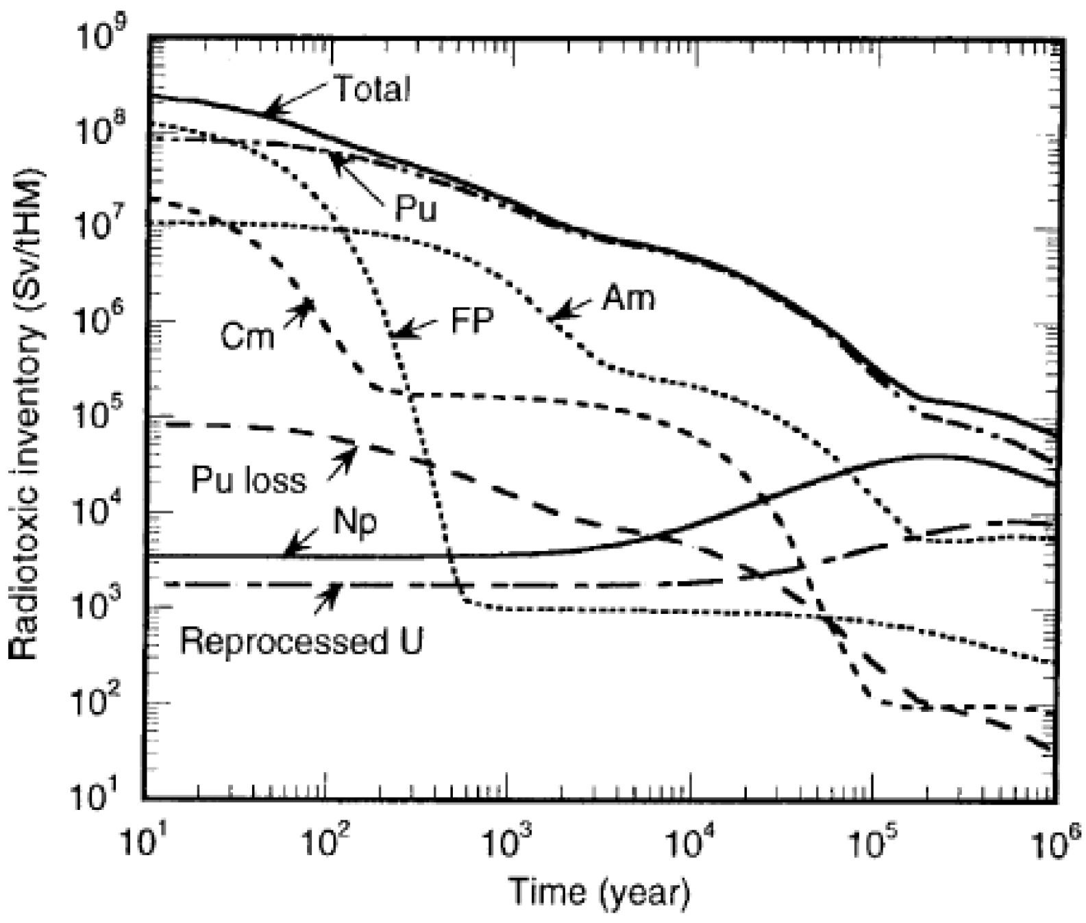
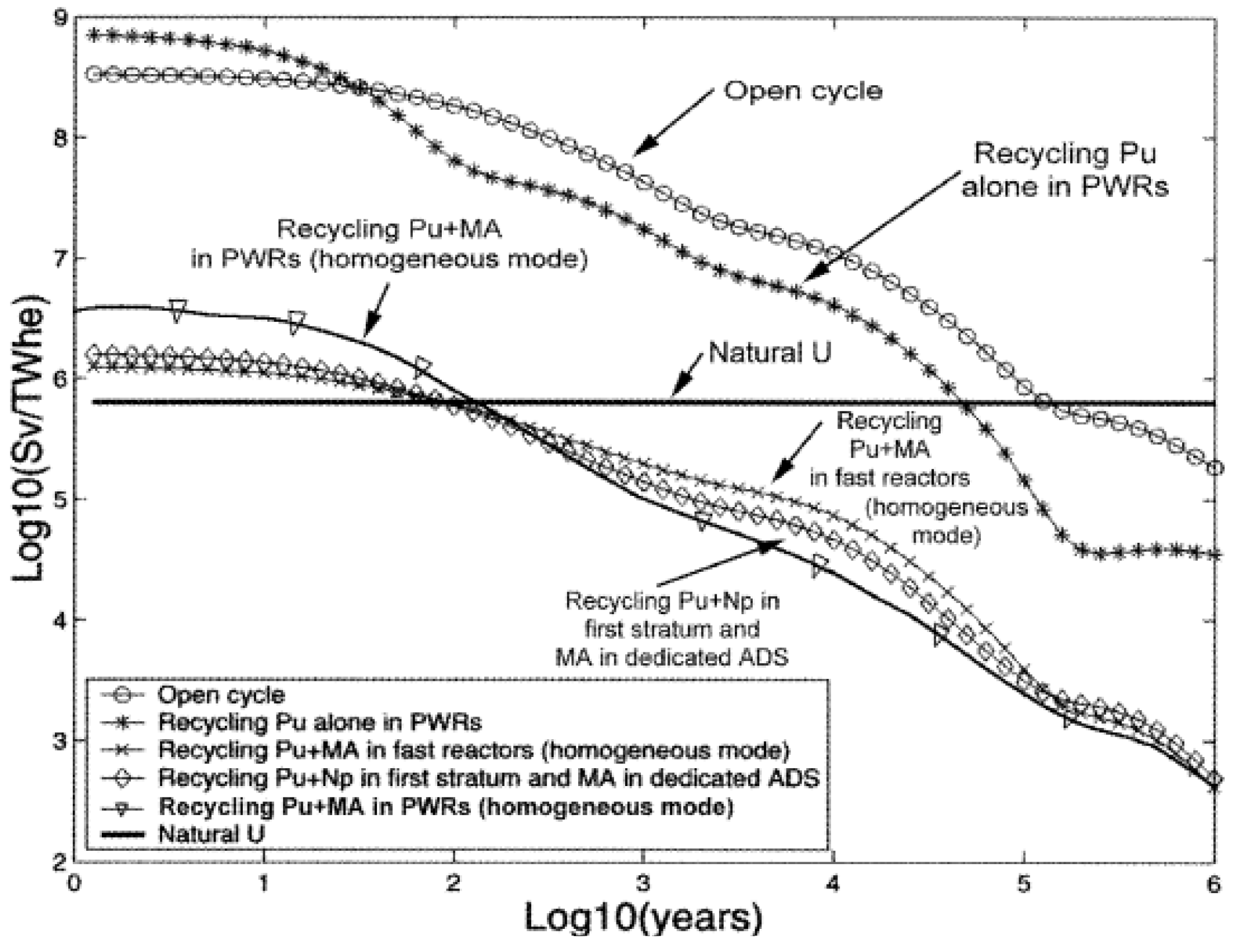
5.4.1.9. Transmutation

Nuclear transmutation is the conversion of one isotope into another facilitated by nuclear devices such as particle accelerators or fission reactors. Transmutation of transuranium elements (TRU) such as the isotopes of plutonium and minor actinides (MA; neptunium, americium, and curium, see Figure 32) has the potential to help solve the problems posed by the management of radioactive waste, by reducing the proportion of long-lived isotopes it contains, and by reducing the overall amount of waste destined for geological disposal. Removing only plutonium would reduce overall radiotoxicity by 90%. Effectively dealing with plutonium as well as the minor actinides would reduce overall radiotoxicity by 99%, and would mean that remaining waste could reach ore level activity after a few hundred years [152]. There would be a build-up of curium during multirecycling of plutonium and minor actinides, however because of its relatively short half life, curium could be stored temporarily and re-introduced into multirecycling after a significant part has decayed. When irradiated with fast neutrons, these isotopes can be made to undergo nuclear fission, destroying the original actinide isotope and producing a spectrum of radioactive and nonradioactive fission products.

Salvatores [152,153] describes various strategies for large-scale deployment of transmutation. They can be classified according to whether (a) fast reactors are part of the future reactor suite, and whether: (b) plutonium is being regarded as a fuel or as waste. If only thermal reactors were available and plutonium is regarded as fuel, then plutonium produced by ordinary UOX thermal reactors can be partitioned from the spent fuel, and recycled by using MOX in PWR (heterogeneous recycling). However, thermal reactors are not as efficient as fast reactors (because of the neutron capture in U-238 and because of the high capture-to-fission ratio of actinides for thermal neutrons; Table 1 in [115]), and also need would need to increase their U-235 enrichment (Tables 1 and 2 in [154]). The neutron capture of U-238 and subsequent breeding of new actinides can be eliminated by using Inert Matrix Fuels (IMF) where the fertile U-238 is replaced by a neutron-transparent matrix. IMFs can therefore greatly enhance efficiency of actinide transmutation in thermal-neutron reactors [155,156,157]. At the end of the recycling stages, both plutonium (from MOX) and minor actinides (from both MOX and UOX burning) can be transmuted together in a dedicated transmuter plant (so-called double-strata strategy). If only thermal reactors were available and plutonium is regarded as waste, then both plutonium and minor actinides produced by ordinary UOX thermal reactors would be directly transmuted together in a dedicated transmuter plant. These transmuter plants would likely be sub-critical accelerator-driven systems because critical systems with actinide-dominated fuel have an unfavourably high reactivity because of the low fraction of delayed neutrons. If Gen-IV fast reactors were available, then both plutonium and minor actinides produced by ordinary UOX thermal reactors would be directly transmuted in those (homogeneous recycling). In all cases, the only materials ever being sent to a waste repository would be losses from partitioning, transmutation and recycling (in the order of 0.1%–1%; [154]). Also, whatever the option, reprocessing and/or transmutation always reduces the long-lived waste components (see Figure 33).

Figure 32. Radiotoxic evolution of a UOX reactor inventory over time, showing the long-term dominance of plutonium, followed by americium, curium and neptunium (Figure 1 in [154]), thus indicating the benefits of transmutation. Fission products (FP) contribute radiotoxicity only up to 500 years. © 2005 Elsevier, reproduced with permission.

Figure 33. Radiotoxicity evolution with time for different scenarios of partitioning and transmutation. (Fig. 5 in [115]). Plutonium recycling alone reduces radiotoxicity by a factor of 3, but additional recycling of MA leads to about 300-fold reductions. © 2002 Elsevier, reproduced with permission.

5.4.2. Capacity and load characteristics

Given the high load factors of Generation-II and -III plants, it is reasonable to expect that Generation-IV plants would operate at 90% capacity.

5.4.3. Life-cycle characteristics

Tokimatsu et al. [110] carry out a life-cycle assessment for a LWR system and a breeder fuel cycle, arriving at 12 g CO₂/kWh and 5 g CO₂/kWh, respectively. The LWR values are significantly below those reported by Lenzen [34], because [110] do not include emissions from mining. They also undertake a dynamic analysis of four scenarios for Japan, ranging from the rapid promotion of breeders to total phase-out of nuclear power. They show that over a period of 65 years, LWR avoid about 25 Gt CO₂ compared to a phase-out scenario, and breeders avoid 300 Mt CO₂ compared to LWR. No life-cycle studies for other generation-IV reactor types could be located.

5.4.4. Current scale of deployment

Generation-IV plants are developed under the guidance of the Generation-IV International Forum, comprising the main nuclear-generating nations [149]. No plants have yet been deployed. The initial Molten Salt reactor (MSR) reference design is planned at a scale of 1,000 MWe with a deployment target date of 2025. Based on the state of development and research needs, transmuter plants could be deployed starting 2030 (Section 3 in [153]). Advanced plants have been proposed at scales between 24 MW (MPBR) and 1600 MW.

5.4.5. Contribution to global electricity supply

Generation-IV systems are not expected to begin commercial electricity production before 2040 (Figure 34). Only VHTR and SFR are currently considered to be of high feasibility (Table 5; [149]), with the SFR potentially hindered by public opposition. This was also the outcome of an evaluation by 100 GIF-member experts [133].

5.4.6. Cost of electricity output

Even though fast breeder reactors remain the strategic direction of the power program of Japan, cheap supplies of “off the shelf” uranium and especially of enriched uranium have made current FBR technology uncompetitive with PWR and other thermal reactor designs. PWR designs remain the most common existing power reactor type and also represent most current proposals for new nuclear power stations.

Figure 34. Subsequent generations of nuclear power plant concepts. © OECD Nuclear Energy Agency, reproduced from http://www.gen-4.org/Technology/evolution.htm.

Lim et al. [45] briefly report results from a US study (MIT) stating that cost for advanced nuclear cycles are considerable higher than those for existing once-through cycles, and that therefore advanced technologies are not expected to be competitive before at least 2050.

Dedicated transmuter systems for the reduction of minor actinide waste require subcritical systems (for example ADS), because the high reactivity of reactor cores loaded with significant actinide content makes it potentially unsafe to use critical systems. This circumstance will add to the cost of any system involving dedicated transmutation. It is not known how these costs would stack up against the savings made in terms of reduced volumes of geological storage (compare Section 4a in [152]).

The GIF (www.gen-4.org/Technology/horizontal/economics.htm) has implemented Cost Estimating Guidelines for Generation IV Nuclear Energy Systems as a living document that has been updated numerous times over the past several years, and that is an outlet of the Economic Modeling Working Group’s work to create an integrated nuclear energy economic model for application to Generation IV nuclear energy systems. With continuing R&D, cost of Gen-IV reactors will become clearer.

5.4.7. Technical challenges

Amongst the GIF’s priority goals, fast reactors generally have low potential for passive safety, however they produce less fissile waste than other types, exploit better the nuclear energy in the fuel, and also allow for transmutation of long-lived isotopes into short-lived isotopes. Only VHTR and GFR have the ability to generate high-temperature heat (Table 5). The VHTR also stands out in terms of potential for passive safety, which is due to the temperature resistance of the fuel elements.

**Table 5.** Potential of reactor design to meet different Generation-IV goals. © 2008 Elsevier, reproduced with permission from [149].
Generation-IV goal	VHTR	GFR	SFR	LFR	SCWR	MSR
Efficient electricity generation	Very high	High	High	High	High	High
Flexibility: availability of high-temperature process heat	Very high	High	Low	Low	Low	Low
Sustainability: creation of fissile material	Medium/low	High	High	High	Low	Medium/low
Sustainability: transmutation of waste	Medium	Very high	Very high	Very high	Low	High
Potential for “passive” safety	High	Very low	Medium/low	Medium	Very low	Medium
Current technical feasibility	High	Medium/low	High	Medium	Medium/low	Low

The PUREX technique to reprocess breeder blankets is generally seen as a large proliferation risk because in principle plutonium can be obtained for weapons manufacturing. For this reason, fast breeder fuel cycles are generally considered less proliferation-resistant than once-through fuel cycles. These problems may be solved with the introduction of new reprocessing methods such as pyroprocessing [13].

Very high temperature and fast reactor designs require the development of high-temperature and irradiation-resistant alloys that allow vessels and turbines to operate at elevated temperatures and neutron fluxes [158,159]. MPBR designs are often challenged because of the presence of graphite, which could potentially ignite. Furthermore, the inability to re-process the fuel pebbles means that MPBRs increase storage problems. In general, the behaviour of the coated pebbles and the structural graphite under irradiation is not yet satisfactorily understood [149]. Molten salt reactors face problems related to the corrosiveness and biotoxicity of the salts, and potential positive reactivity coefficients and degradation of the graphite moderator. In liquid-metal-cooled fast reactors the opaque coolant prevents easy core inspection and maintenance. Gas is a relatively poor coolant, so that gas-cooled fast reactors need large core masses provided thermal inertia (http://www.gen-4.org/Technology/ systems/gfr.htm; [149]). Whilst avoiding phase changes and allowing direct turbine feed, supercritical water-cooled reactor designs must deal with the high corrosiveness of supercritical water.

The Thorium fuel cycle requires remote fuel handling because of short-lived decay products that are intense gamma emitters. The challenges for developing transmuter plants are the relatively high neutron doses required in transmuter fuel to fission minor actinides, thus requiring remote handling, and the lack of experience with minor actinide behaviour under neutron irradiation [153]. Also some fission products such as technetium, iodine, strontium and caesium cannot be transmuted easily because of their low cross-sections [115]. These isotopes have half lives between decades and a few hundred years, and it is recommended that they be stored to decay.

It is generally thought that the advanced nuclear fuel cycle technologies listed above may take decades of R&D efforts in the fuel cycle as well as operation before implementation (p.10 in [146], p. 54 in [1]).

6. Hydroelectric Power

6.1. Summary

Hydropower exists as a “large” (mostly dammed) and a “small” (mostly run-of-river) technology option, with the dividing line at about 10 MW capacity. These plants operate with intermediate load factors of around 40%, serving both base and peak loads. Hydropower’s ability to come on line within a few minutes makes it an excellent option to capture demand peaks. Whilst large hydropower installations built over the past decades represent more than 90% of the world’s current capacity, and supplying about 17% of the world’s electricity, they are also associated with major environmental and social impacts, leading to a significant decrease of recent funding. On the other hand, small hydropower is seen as environmentally benign, and able to alleviate poverty and foster sustainable development especially in remote communities in developing countries. Hydropower installations in general are characterized by very low operational cost, but high upfront capital cost, often preventing construction or capacity expansion investment. Once capital costs are recouped, however, hydropower has extremely low operating cost. Significant economies of scale make small installations less economical at levelised electricity cost between 5 and 20 US¢/kWh, compared to large hydropower at 5–10 US¢/kWh. Life-cycle greenhouse gas emissions for large hydropower installations can reach up to 200 g/kWh in case of substantial anaerobic decay of submerged plant matter. Existing old plants, as well as new small hydro plants have however smaller emission factors around 40 g/kWh. Assuming a global resource potential of up to 6–10 PWh/year, hydropower could avoid up to 300–400 Gt CO₂ until 2100.

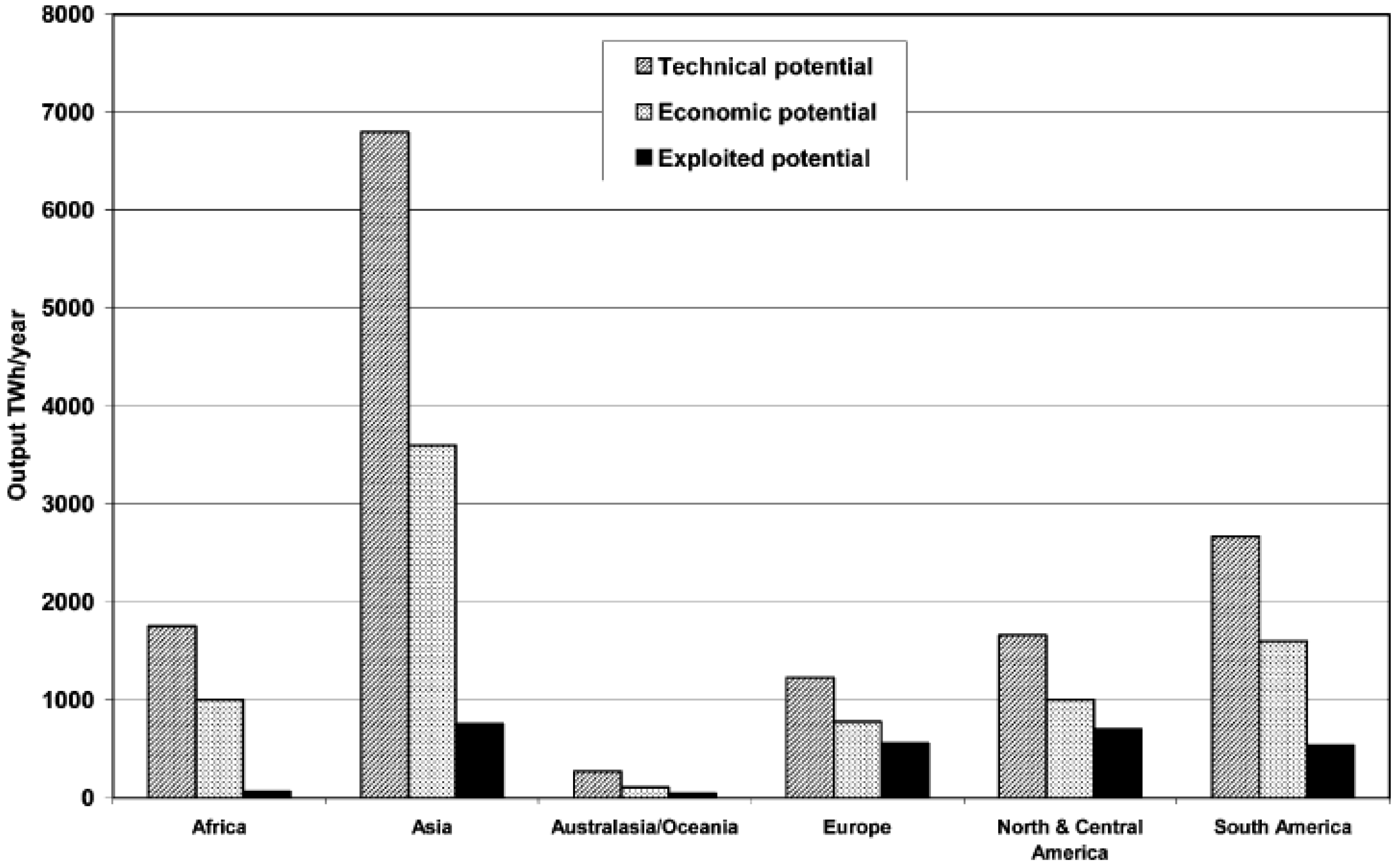
6.2. Global Potential of Resource

Between 1970 and about 2006, hydro electricity production has experienced a continuous increase (Figure 35). This increase has been less pronounced though compared to the initial rise of nuclear power.

Figure 35. Evolution of hydro electricity production by region (after [17]). Asia excludes China.

The reason for this circumstance is that many large hydropower projects are associated with significant environmental harm and social disruption. As a consequence, international funding for large projects has been substantially reduced [160]. In some areas, especially in Europe, the most cost effective sites have already been exploited [1,161]. This leaves as options the dispersed expansion of new small hydro projects, the uprating of hydropower facilities at existing large dams, and the retrofitting of existing non-hydro dams [160].

The world’s total feasible hydro potential is estimated at close to 15 PWh/year, of which about 8 PWh/year are estimated to be economically feasible ([46]; Figure 36). Almost half of the latter potential exists in Asia (1.75 PWh/y alone in China 20% of which as small hydro applications, [162]; 1 PWh/year alone in India, 10% of which as small hydro, [49,163]), 20% in Latin America, and 15% each in Africa, and North and Central America. This means that the production of hydropower electricity could in principle increase two- to three-fold (compare [2], p. 387). Small hydro potential is estimated at more than 1 PWh/year, occupying about the same fraction in the current and potential total hydropower supply [164], however estimates vary considerably. Kosnik [160] reports a 1 PWh/y potential of small hydro in the US alone, compared with only 25 and 120 TWh/y, respectively, for uprating and retrofitting existing facilities in the US. However, Hall et al. in [165] arrive at only about 0.6 PWh/y for all (small and large) hydro resources for the US.

Interestingly, mainly developing countries would benefit from future hydropower development, such as the Democratic Republic of the Congo and Cameroon which feature Africa largest hydropotential resources [166]. In fact, there are plans for two new hydroelectric stations at the Congo River with a combined output of more than 40 GW, producing 370 TWh annually. This would be a significant addition to the entire African continent, which in 2005 produced 550 TWh of electricity (600 kWh per capita, compared to 2000 kWh/cap in Brazil, and around 4000 kWh/cap in the OECD).

Hydropower is seen as a large avoider of greenhouse gas emissions. Generating the current annual amount of electricity using the 2006 fossil fuel mix would cause about 3 Gt CO₂ annually, so that continuing all current hydropower operations until 2100 would avoid about 250 Gt CO₂. If all additional economically large hydropower sources were to replace the current fossil fuel mix, and accounting for the increased emissions from submerged biomass from new plants, an additional 300 Gt CO₂ could be avoided by 2100 (Kosnik [160] estimates the emissions saving potential in the US alone to be about 2.9 Gt/y). A similar estimate for small hydropower is difficult to arrive at because of varying estimates of the global potential, but assuming a possible contribution of 1 PWh/year, small hydro would avoid just under 1 Gt CO₂ annually, and below 100 Gt CO₂ until 2100. However, these savings reduce if more renewable enter the overall electricity mix. A realistic estimate for both large and small hydro is perhaps 300–400 Gt CO₂ for this century.

6.3. Dam and run-of-river plants

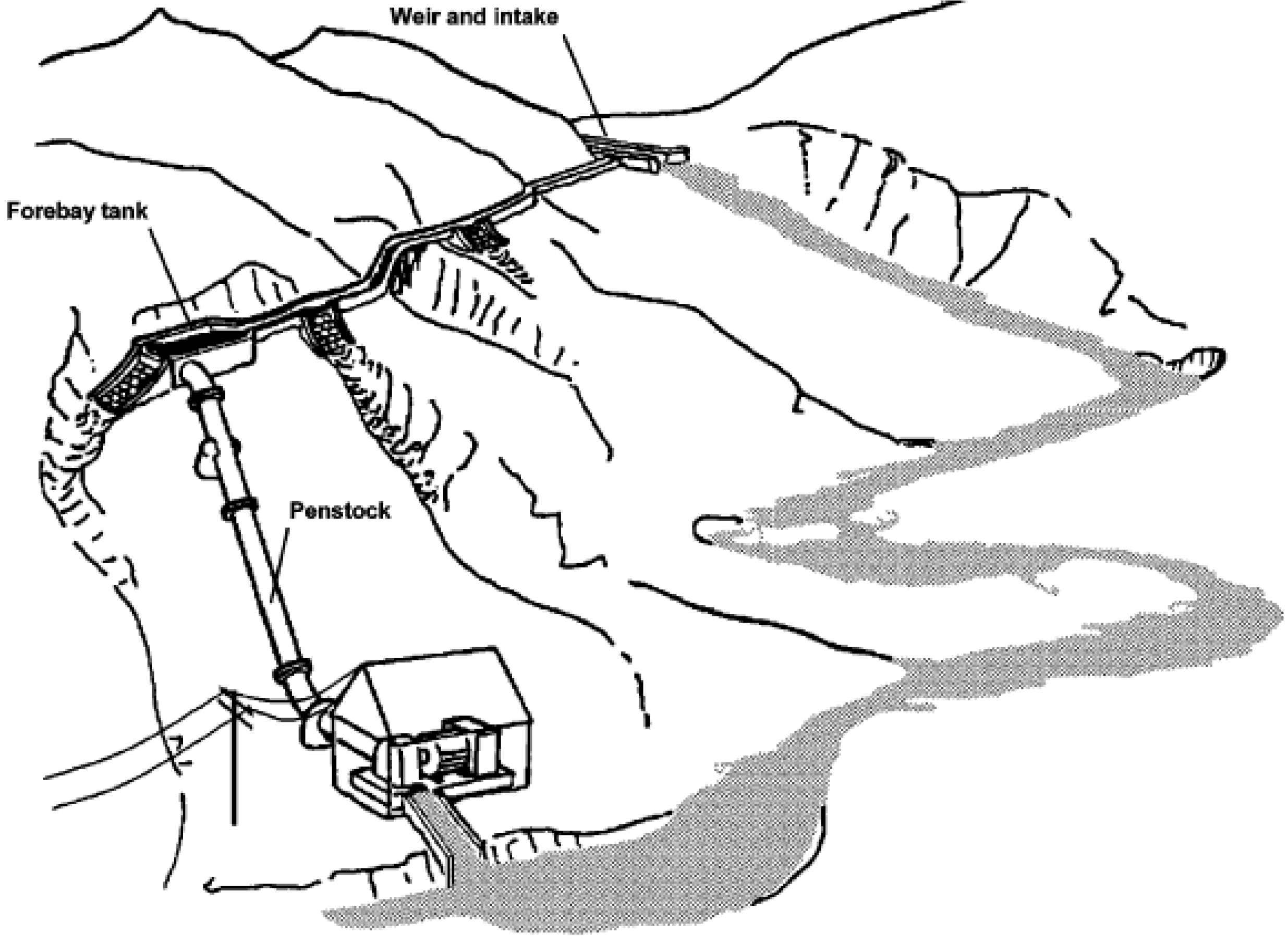
6.3.1. Technical principle

Hydroelectric power comes from damming or diverting of a waterway into a penstock feeding a water turbine [167]. Most hydroelectricity in the world is generated in dam type stations. In this case, the energy generated from the hydraulic potential depends on the water volume and on the difference in height (the “head”) between the reservoir and the turbine. Smaller hydropower installations are often of the diverting, or run-of-the-river type [164], where the natural flow of a (preferably continuously flowing) river is used to generate electricity. In contrast to dam installations, run-of-river projects do not lead to large flooded areas. A pure run-of-the-river power plant cannot store energy and hence cannot match consumer demand.

Pumped storage hydroelectricity is a term used for a plant that is able to pump water into a reservoir uphill during times of low demand, and to be used in times of peak load. Because of the low energy density of pumped storage systems, a large body of water or a large variation in height is needed to create significant energy storage. Reversible turbine/generator assemblies act as pump and turbine [168]. Pumped storage is a net consumer of energy (taking into account evaporation losses from the exposed water surface and conversion losses, approximately 70% to 85% of the electrical energy used to pump the water into the elevated reservoir can be regained), but generally a net generator of revenue, because power is sold at peak-load prices, thus permitting base load power stations to continue operating at optimum efficiency, and leveling the fluctuating output of variable power sources. Pumped storage schemes currently provide the only commercially important means of large-scale grid energy storage and improve the daily load factor of the generation system.

Small hydro is the term used for mostly run-of-river plants up to 10 MW rated capacity (Figure 37), which are usually applied to dedicated industrial plants or to small communities. Small hydro includes a range of sub-terms such as mini hydro (<1 MW), or micro hydro (<100 kW). The latter are applied in very small communities, often in remote areas that would be uneconomic to supply from a grid. Small hydro projects are characterized by small infrastructure and hence low construction cost and low environmental impact, which makes the ideally suited for deployment in developing countries where electrification is still low (see case studies from Cameroon: [166]; India: [49,163]).

The International Energy Agency has formed working group called the Hydropower Implementing Agreement with a common interest in advancing hydropower worldwide (www.ieahydro.org). This working group disseminates information on hydropower, and organises and promotes activities and implementation.

6.3.2. Capacity and load characteristics

The chief advantage of hydroelectric dams is their ability to handle seasonal (as well as daily) high peak loads. Unlike other sources, additional hydropower can be fed into grids with start-up times in the order of a few minutes (spinning and non-spinning reserves; [46]), and load changes can be compensated within seconds. In 2006, 3,121 TWh of hydroelectricity were generated with 867 GW installed capacity, yielding a load factor of 41% [17]. Load factors of large hydroelectric plants vary between 25% and 75% (Table 6), depending on whether they are operated more as base-and-peak-load (in countries with abundant hydro resources) or more as peak-load plants (in countries with less abundant hydro resources; [167]). In general, small hydro plants utilize the entire water potential available to them, and are therefore often characterized by high load factors in comparison to larger systems [161,164]). Because of its excellent ability to meet short-term demand swings, hydro power is often seen as an ideal renewable technology to meet load imbalances in systems with large variable-source penetration (wind, solar, etc., see Section 6.3.2).

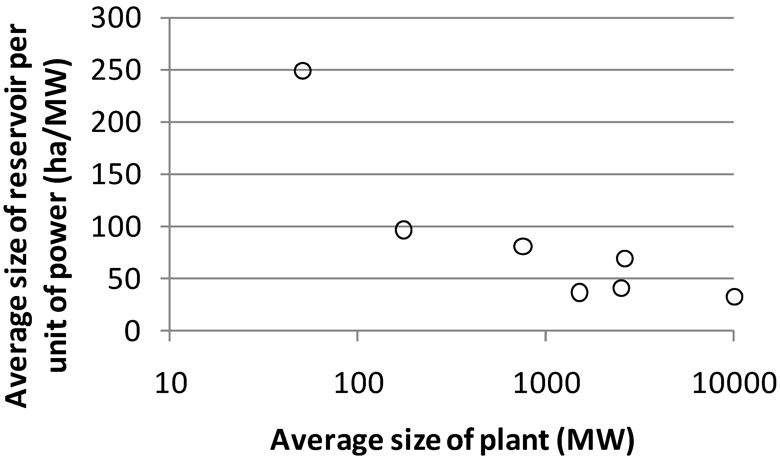
6.3.3. Life-cycle characteristics

Lenzen et al. [47] include a literature review of life-cycle energy consumption and greenhouse gas emissions of hydropower. Greenhouse gas emissions range from 1–5 g/kWh for run-of-river plants, and from 5–60 g/kWh for reservoir plants. Lenzen et al. [47] undertake a sensitivity analysis for Australian conditions and arrive at conservative estimates for life-cycle energy of 0.02–0.14 kWh_th/kWh_el, and for life-cycle emissions of 7–45 g/kWh. These values agree with the existing literature. Depending on the vegetation of the flooded area, the reservoirs of power plants may emanate methane and carbon dioxide stemming from the decay of plant material in an anaerobic environment. The global warming effect occurs because the organic matter would have decayed into a larger fraction of CO₂ and less CH₄, had it decayed in an aerobic environment above water (see [169,170,171]). Dos Santos et al. [48] measured these emissions at a number of Brazilian hydro reservoirs and concluded values of around 200 g/kWh. Rashad and Ismail [172] report even higher greenhouse gas emissions of 410 g/kWh from Egypt’s Aswan power station. These emissions do not stem from anaerobic decay of plant matter (Aswan’s surrounding are extremely arid desert), but from two large fertilizer plants that compensate the loss of sedimentation downstream from the dam. Lima et al. [173] report on simulations about methane emissions downstream from the dam, brought about by a “degas drop-pressure effect” that arises when CH₄-saturated water passes through turbines, and that leads to CH₄ bubbling-out immediately downstream of the dam. Lima et al. [173] estimate this proportion to be much larger than the upstream CH₄ emanating from the reservoir surface, though most of the downstream CH₄ emissions would be recoverable and convertible to useful energy. Note that these findings are based on simulations and have to be confirmed by measurements.

6.3.4. Current scale of deployment

Most of the world’s capacity of 867 GW resides in the China (118 GW), followed by the United States (99 GW), Canada (72 GW), Brazil (71 GW), Japan (47 GW), Russia (46 GW), India (35 GW), Norway (28 GW), France (25 GW), and Italy (21 GW). A few percent of this capacity is in form of pumped storage. Large hydroelectric installations generate most of the world’s hydroelectricity. Table 6 provides a list of the largest hydropower stations at the time of writing.

The Three Gorges Dam project in Hubei, China, is the world’s largest hydroelectric generating system, including two generating stations, with a rated capacity of this complex is 22.5 GW ([162], Table 6). New large hydro constructions are underway for example in India (8 GW), China (more than 50 GW), and Brazil (6GW) [65]. On the other end of the scale, less than 10% of the world’s hydropower capacity, or about 70 GW, was installed as small hydro installations, ranging from several kW to 10 MW rated plant output. This percentage is relatively constant across regions (Europe – [174]; India – [49,163]; Greece – [161]; Spain – [175]), except for China, where small hydro accounts for about 35% of total hydroelectricity generation [162]. Most of small hydro (39 GW) is in China, followed by Japan (3.5 GW) and the United States (3 GW), and India (1.5 GW).

A debate exists about the preferred deployment scale [46], with small run-of-river hydro being perceived as having smaller social and environmental impacts [176,177]. Critics respond that impacts have to be judged per unit of service from plants [167].

Table 6. List of the largest hydroelectric power stations (en.wikipedia.org/wiki/List_of_the_largest_hydroelectric_power_stations).

**Table 6.** List of the largest hydroelectric power stations (en.wikipedia.org/wiki/List_of_the_largest_hydroelectric_power_stations).
Name	Country	Year of completion	Total Capacity (MW)	Max annual electricity production (TWh)	Area flooded (km²)	Load factor (%)
Three Gorges	China	2009	22,500	>100	632	62
Itaipu	Brazil/Paraguay	1984/1991/2003	14,000	90	1,350	73
Guri	Venezuela	1986	10,200	46	4,250	51
Tucuruí	Brazil	1984	8,370	21		29
Robert-Bourassa	Canada	1981	7,722
Sayano Shushenskaya	Russia	1985/1989	6,400	26.8		48
Krasnoyarskaya	Russia	1972	6,000	20.4	2,000	39
Grand Coulee	United States	1942/1980	6,809	22.6		38
Churchill Falls	Canada	1971	5,429	35	6,988	74
Longtan Dam	China	2009	4,900	18.7		34
Bratskaya	Russia	1967	4,500	22.6		57
Ust Ilimskaya	Russia	1980	4,320	21.7		57
Yaciretá	Argentina/Paraguay	1998	4,050	19.2	1,600	54
Tarbela Dam	Pakistan	1976	3,478	13		43
Ertan Dam	China	1999	3,300	17.0		59
Ilha Solteira	Brazil	1974	3,200
Xingó	Brazil	1994/1997	3,162
Gezhouba Dam	China	1988	3,115	17.01		62
Nurek Dam	Tajikistan	1979/1988	3,000	11.2		43
La Grande-4	Canada	1986	2,779
W.A.C. Bennett	Canada	1968	2,730
Chief Joseph	United States	1958/73/79	2,620
Volzhskaya	Russia	1961	2,541	12.3		55
Niagara Falls	United States	1961	2,515
Paulo Afonso IV	Brazil	1955	2,462
Chicoasen	Mexico	1980	2,430
La Grande-3	Canada	1984	2,418
Atatürk Dam	Turkey	1990	2,400	8.9		42
Zhiguliovskay	Russia	1957	2,300	10.5		52
Iron Gates-I	Romania/Serbia	1970	2,192	13		68
Caruachi	Venezuela	2006	2,160	12.95		68
John Day Dam	United States	1971	2,160
Aswan	Egypt	1970	2,100	11		60
Itumbiara	Brazil	1980	2,082
Hoover Dam	United States	1936/1961	2,080
Cahora Bassa	Mozambique	1975	2,075
The Dalles Dam	United States	1981	2,038
Karun I Dam	Iran	1976	2,000
Karun II Dam	Iran	2001	2,000
Karun III Dam	Iran	2007	2,000	4.1		23
Lijiaxia Dam	China	2000	2,000

6.3.5. Contribution to global electricity supply

Electricity from hydropower grew from 1295 TWh in 1973 to 3121 TWh in 2006 ([17]; Figure 35). Estimates of the contribution from small hydro projects vary [164,178], but 250 TWh/year is probably a realistic estimate for small hydro worldwide, given that China alone produced nearly 100 TWh/year [50]. In 2006, more than 40% of nuclear power generation occurred in OECD countries (down from more than 70% in 1973), about 21% each in Latin America and Asia, and about 8% in the Former Soviet Union.

In 2006, hydropower plants provided 16.4% of the world’s electricity [17]. Regional shares vary widely, with Norway leading at 99%, followed by Brazil (83%), Venezuela (72%), Canada (58%), Sweden (43%), Russia (18%), India and China (both 15%), Japan (9%), and the United States (7%). Latin America is the continent with by far the highest share of hydropower in the electricity mix (66%; [160]).

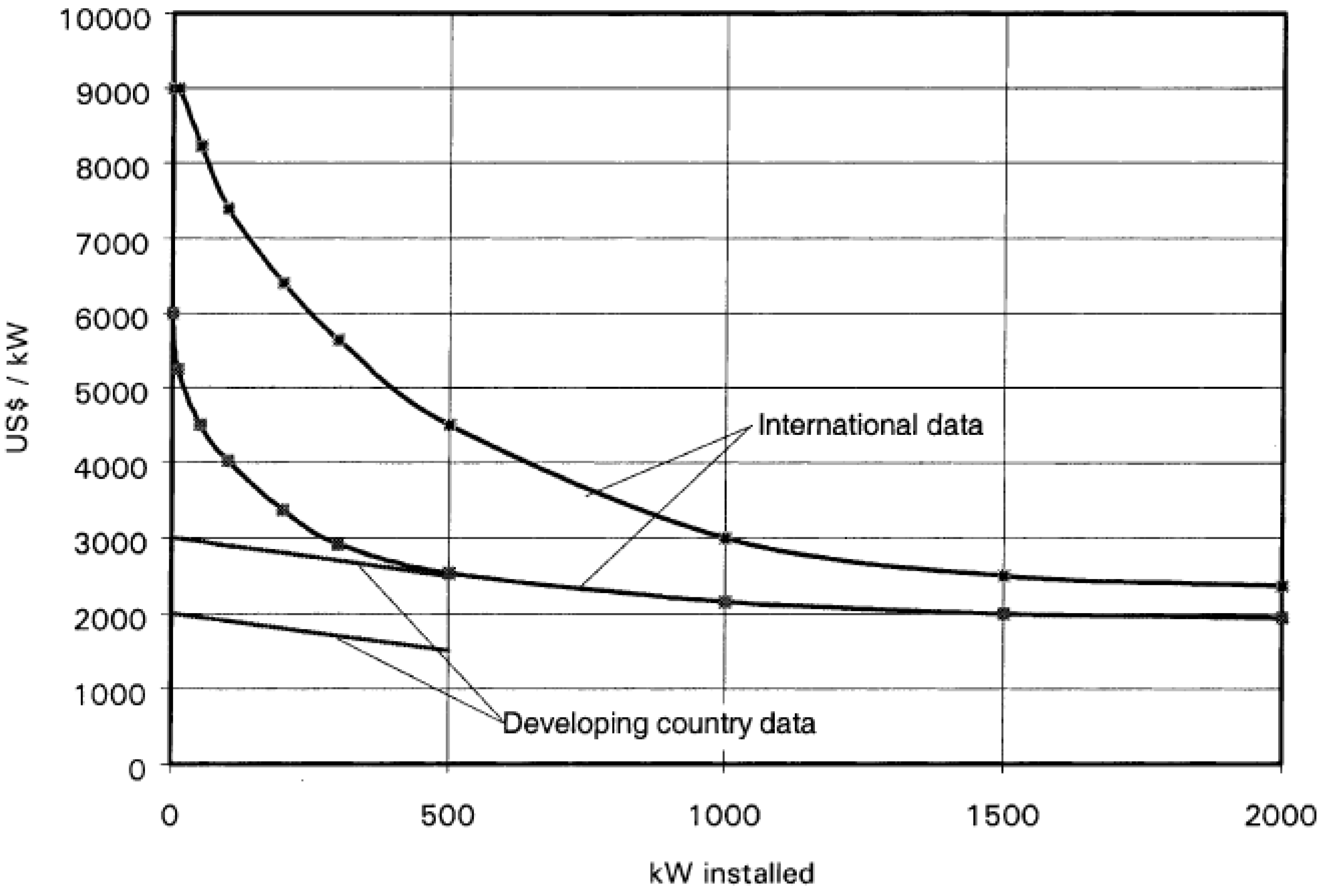
6.3.6. Cost of electricity output

Upfront capital cost that are the main component of hydropower’s electricity cost, mainly because of long lead-times created by requirements for site studies, hydrological studies using long-term data, and environmental impact assessment. These circumstances create significant investor risk. On the other hand, the main advantage of hydroelectricity is the absence of fuel cost, and therefore the independence from the prices of fossil fuels such as oil, gas and coal. Hydroelectric stations have long operational lives of up to 50–100 years. Labour costs are also low because of the high degree of automation. However, hydropower depends on rainfall, and may be severely restricted during periods of drought. Therefore, hydropower station operators add storage capacity in order to accommodate for periods of low water availability. This can also facilitate the ability to withhold energy supply for future use. Nevertheless, in contrast to thermal power plants, hydropower operators must deal with a resource endowment that is given but unknown in advance throughout any one year, and strategically optimise their output across periods based on inflow expectations. There is hence an opportunity cost associated with any water release [179]. In economies that feature a large percentage of hydropower such as Brazil, electricity markets are structured that variable cost for hydroelectricity determine the spot price, and often outcompete fossil-fuelled electricity, but average costs are much higher and prevent adequate capacity expansion in case of deregulation, leading to shortages in the long term [180].

The unit electricity costs of small-scale hydro projects suffer from significant economies of scale in the form of fixed cost from feasibility studies and other overheads ([181]; Figure 38).

In a survey by the OECD NEA and IEA [31] of micro hydropower plants, levelised electricity cost were between 4 and 8 US¢/kWh at 5% interest rate, and between 6.5 and 10 US¢/kWh at 10% interest rate. In general, the higher the capacity factor, the better the internal rate of investment return [161]. Levelised electricity costs are strongly dependent on the system scale: Micro-hydro projects in India were costed between 10 and 20 US¢/kWh [49], but small hydro power in China has levelised electricity cost of about 4 US¢/kWh [50]. The latter estimate is probably more realistic for mature-technology prices, since China has by far the most small hydro installations, which are to a large extent connected to the grid and are hence competing with thermal plants. However, Zhou et al. [50] warn that with time, more and more uneconomical sites are exploited, driving up electricity cost. The small project size and revenue streams also mean high risk with regard to unforeseen events. Joint development of a number of small projects is seen as beneficial, as is the standardization of technologies into “water-to-wire packages”. Both strategies avoid application-specific re-engineering and associated cost. Notwithstanding the challenges, small hydropower is economical especially in remote settings, for example on islands (see for example [161], and also [182] and references therein). In combination with wind power, small hydro can even out supply fluctuations, and in cases provide up to 90% of island power [183].

In general multipurpose uses such as irrigation, flood control, water supply, navigation and recreation (¹/₃ of all hydropower projects; [167]) can assist in reducing electricity cost from hydropower [184].

6.3.7. Technical and other challenges

Hydropower developments have been the subject of intense social and environmental concerns (see for example [185,186]). The main issues are [160,187]

–: displacement of residents from flooded areas,
–: transformation of traditional land use,
–: sedimentation and eutrophication of reservoirs, scouring of downstream riverbeds,
–: disturbance and fragmentation of faunal habitat, obstruction of fish passage, thermal pollution, disruption of reproductive cycles, and changes in fish species composition,
–: large accidental dam failures or purposeful attacks on large dams.

Because of the intense media attention it attracted, Egypt’s Aswan dam has at times been described as “the most popular environmental problem in the world” [172]. Rapid reservoir siltation, loss of fertility and increase of salinity of soils, downstream erosion occurred because of the dam’s operation, the latter even in Egypt’s Nile Delta, where the reduced silt deposition led to increased sea erosion. Large hydropower projects planning with little consideration for environmental and social impacts is not an exception, as an internal World Bank survey has demonstrated [172], although this could be improved by applying proper social impact assessment practices [188] and institutional settings [189]. On the other hand, these social and environmental issues are often contrasted with very similar developments that would occur under advanced climate change [46]. Further arguments make the case that the impacts from non-hydro dams are similar to those of hydro dams, and equal environmental criticism should be directed towards such water supply facilities [190]. Finally, Égré and Milewski [167] point out that damages have to be judged on a per-unit-of-service basis, and argue that the difference in impacts from one large dam or hundreds of small hydro projects are less obvious. These authors present average surface areas of reservoirs per unit of power as an decreasing function of size (Figure 39). However, this view may oversimplify issues because it leaves out aspects of thresholds, scale and fragmentation: The argument encapsulated in Figure 39 assumes that impacts are linear with inundated area, however there may be lower thresholds under which there is virtually no impact, not even in a cumulative assessment of many small hydro facilities.

Figure 39. Average size of reservoir per unit of power (ha/MW) as a function of average size of plant (MW) (derived from data tabled in [167]).

Small-scale hydro projects may not be affected as much from these social and environmental considerations, but face their own challenges. Amongst the R&D needs are more detailed and accurate information on hydrology and flow, tools for identifying multipurpose opportunities, the more widespread dissemination of technical and financing know-how, and unit cost reduction for example through further component improvement and standardisation [164,178].

7. Wind energy

7.1. Summary

Wind energy deployment has witnessed a rapid increase throughout the past decade, with annual growth rates around 30%, generating now about 1.5% of global electricity. In recent years, wind power has become competitive without subsidies, in markets without carbon pricing. The global technical potential of wind exceeds current global electricity consumption, however taking into account the temporal mismatch and geographical dispersion of wind energy and demand loads, and requirements for supply-load balance and grid stability, the maximum economic potential appears to be in the order of 20% of electricity consumption [191]. At such rates of wind energy penetration, and without storage and supply-matched demand, the integration of wind power into electricity grids and long-distance transmission begins to present significant challenges for system reliability and loss-of-load expectation. The main issue for future deep penetrations of wind on a global scale is hence how wind plants can be integrated across very large geographical scales and with other variable power sources. For example, there are popular proposals for integrating parts of North African solar power for output-smoothing of large wind supply in Europe [192]. Some commentators remark that these proposals may be difficult to implement because of political and supply security issues [193,194], others [195] are more optimistic. Finally, the life-cycle greenhouse gas emissions from wind power are some of the lowest amongst all electricity generating technologies, but depending on the remainder of the power supply system, emissions arise because of the use of conventional technologies for supply-demand balancing.

7.2. Global potential of resource

In 2008, the global capacity of wind energy converters was 121 GW, generating about 260 TWh of electricity, or about 1.5% of global electricity production [51]. Most of the capacity (Figure 40) is installed in the USA (25 GW) and in the EU (about 65 GW), followed by China (12 GW) and India (10 GW). Wind energy deployment has been increasing rapidly throughout the past decade, recording growth rates of around 30% since 1996 (Figure 41). More than half of the 2008 additions occurred in the USA and in China (Figure 42), with the USA overtaking Germany as the leader in installed wind capacity.

Figure 40. Installed wind power capacity by region (compiled from [51,196]). * Asia excludes China and India.

Figure 41. Historical development of installed wind power capacity, and annual growth rates (compiled from [51,196]).

Measurements from numerous surface and balloon-launch monitoring stations suggest that the global technical potential from onshore wind energy exceeds current world electricity demand [197]. Using global grid-cell data, Hoogwijk et al. [198] undertake a detailed assessment of

-: the theoretical potential (the energy content of global wind),
-: the geographical potential of on-shore wind (excluding land areas with wind speeds below 4 m/s (if the cut-off point had been 6 m/s, areas with current wind turbine installations would have been excluded), and those unavailable for turbine installation, such as nature reserves and areas with other functions urban areas, high altitudes above 2,000 m with low air density (Table 1 in [198] provides suitability factors, which show the percentage of a land area available for wind turbine installation),
-: the technical potential (extrapolating wind data to hub height, considering wake effects and realistic power densities in MW/km², applying average capacity factors, subtracting down time), and
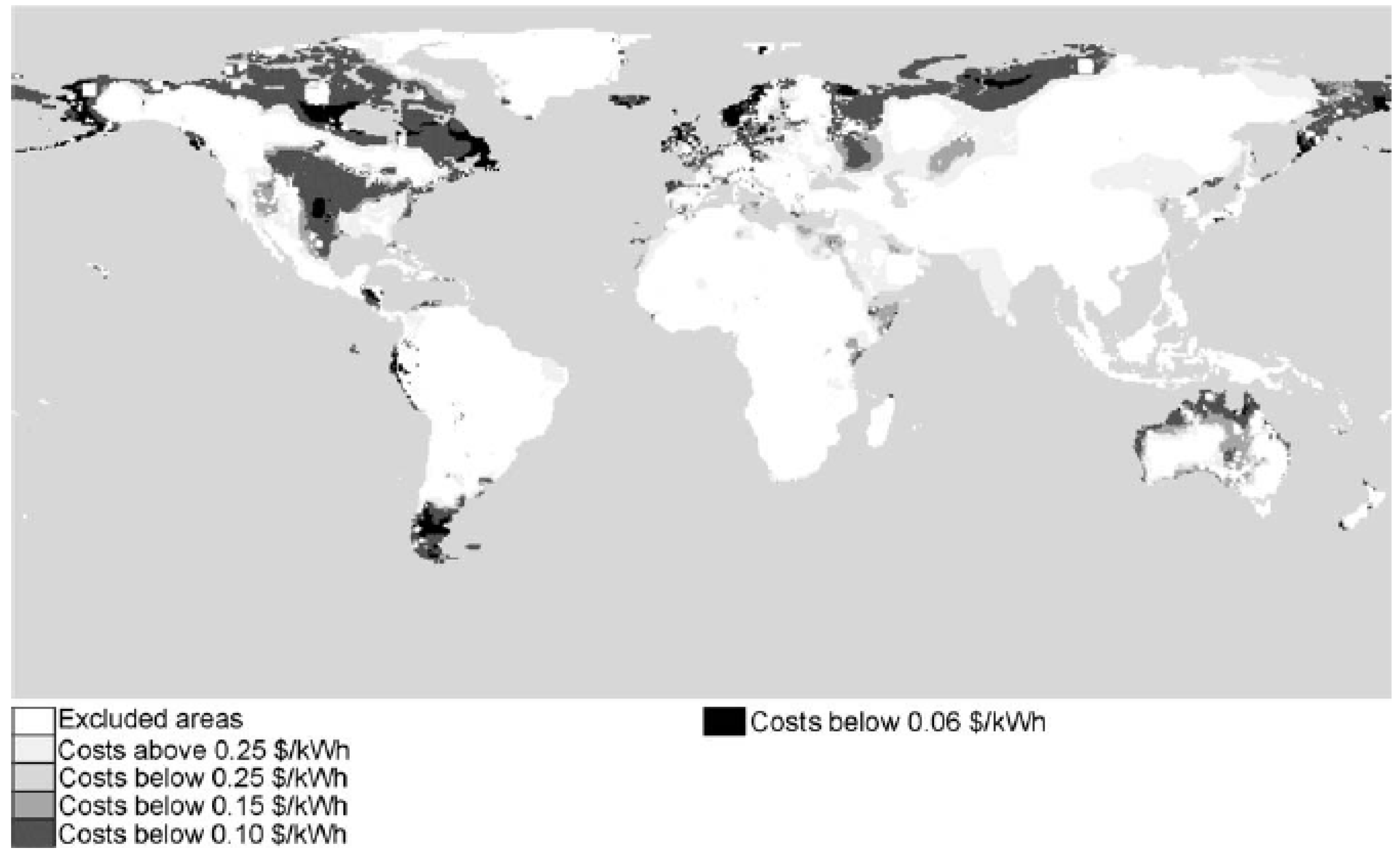
-: the economic potential given cost of alternative sources (calculating rated turbine power optimised for grid cell wind conditions, regressing capital cost and turbine output as a function of rated power and an economies-of-scale factor).

Whilst the theoretical on-shore potential exceeds humankinds energy consumption a few hundred-fold, Hoogwijk et al. [198] estimate the technical potential to be about 100 PWh per year, and the economic potential at cost below 7 US¢/kWh to be about 20 PWh per year, both of which still exceed current global electricity consumption. This is consistent with previous studies ([197], and references listed by [198] in their Section 7.2). However, most of the economic on-shore potential—15 PWh/y—is concentrated in a few remote regions (Figure 43), namely the north of Canada (8 PWh/y), Patagonia (4 PWh/y), Siberia (2 PWh/y), and the coastal regions of Australia (1 PWh/y). Only about 5 PWh/y overlaps with regions of significant electricity consumption, the central US (3 PWh/y), Western Europe (1 PWh/y), and Central America (1 PWh/y). Relatively small potential is found in South and South East Asia. The regional technical potentials given by [198] are confirmed in studies on the USA [199], India [200] and China [201]. Hoogwijk et al. [198] do not include any grid integration, transmission and distribution issues in their assessment, which is instead dealt with in their later publication [191]. The resolution of their global assessment is also such that is cannot account for specific circumstances at the small-region geographical level. In India, for example, the technical potential is further limited by transmission capacity of the grid [200].

Off-shore potential is estimated to be even higher [202], but reliable wind data are often lacking [198]. Off-shore wind power is currently seen as more expensive than on-shore wind, but at higher penetration rates in the longer term could offer more benefits than on-shore because of its more level output, and its proximity to large coastal cities [203].

The later assessment of wind power by Hoogwijk et al. [191] takes into account a whole range of effects occurring with increasing penetration, such as output smoothing and increasing interconnection, depletion of the wind resource, requirements of reliability back-up and short-term spinning reserves, and increasingly discarded excess wind energy.

The potential of wind power is hence not limited by the resource potential, but instead by how much can be integrated into existing power supply systems without causing major supply and demand imbalances, and at acceptable costs [204]. At a given penetration rate, wind power’s mitigation potential would depend on future electricity demand. Assuming steady increases in turbine size (from 1.5 MW in 2007 to 2 MW in 2030) and capacity factor (from 25% in 2007 to 30% in 2030), the GWEC [196] projects a moderate growth scenario to lead to 1400 GW capacity in 2030 (generating 3,500 TWh), and 1,800 GW in 2050 (4,800 TWh). Assuming a 2030 demand of 30 PWh (Section 2.2), this scenario is equivalent to an average penetration rate of just over 11% (compare [196] p. 40). 2050 annual CO₂ mitigation would then amount to about 4.4 Gt CO₂ per year. Extrapolating this trend linearly to 2100 yields a crude estimate of 350 Gt CO₂ total mitigation potential. The GWEC reference scenario yields about 1.7 Gt CO₂/y in 2050, or 150 Gt CO₂ until 2100, and the advanced scenario yields about 8.2 Gt CO₂/y in 2050, or 650 Gt CO₂ until 2100. This is consistent with estimates in [196] (pp. 38,45,46). A long-term global penetration rate of around 20% is perhaps realistic (compare estimates of 15%–20% in [205]) given that (a) large economic potential is not available in all world regions, and (b) current research indicated substantial difficulties of integrating wind at penetration rates of higher than 20% [191]. This corresponds to a total mitigation potential of about 450–500 Gt CO₂. For comparison, Hoogwijk et al. [191] (in their Fig. 14) arrive at potentially avoided CO₂ emissions of 1 Gt CO₂ per year, just in OECD Europe and the USA, at carbon prices of around 30–50 US$/t CO₂. This figure is in the ballpark of the estimate given above.

7.3. Wind energy converters

7.3.1. Technical principle

Wind energy is created by temperature and pressure differences in the earth’s atmosphere. It has been exploited for centuries; there existed thousands of windmills in Europe by A.D. 1800 [206]. There exists a large number of designs for wind energy converters. During the past decade, horizontal-axis three-blade turbines have emerged as the most attractive technology, and today, the majority of commercial wind plants feature machines of this design [196]. The wind energy engaged in the turbine blades is transferred via a rotor to a generator (mostly via a gear box, but sometimes in direct-drive mode), both contained within a housing (the nacelle) situated on top of the turbine tower. Power is transmitted down the tower to a transformer on the ground, and then into the electricity grid. Wind turbines can operate at wind speeds between 3 m/s and 25 m/s, and optimise their performance through rotor yawing and blade pitching, fine-tuned by electronic control and feedback systems. Groups of turbines are often combined into wind farms of sizes between a few to several hundred MW. The largest wind farm, situated in Texas, USA, combined 421 turbines into a 735 MW plant [196]. Wind plants have short construction lead times, even compared to those of transmission infrastructure.

The International Energy Agency’s Wind Agreement (www.iaewind.org) provides a platform for member countries to exchange information on, and experience with research, development, and implementation of wind power. The IEA Wind has several subgroups looking after research tasks such as off-shore deployment or large-scale grid integration.

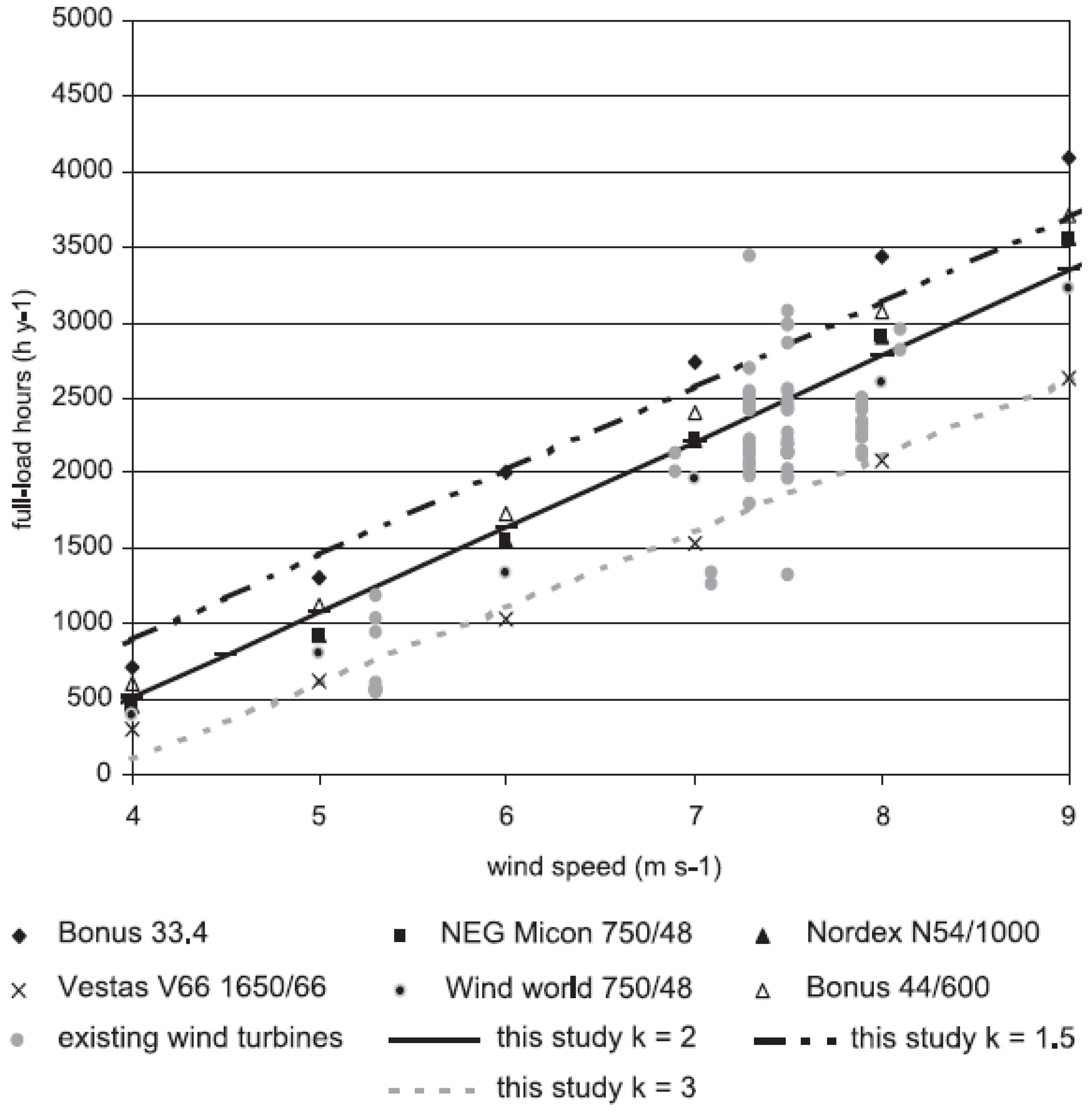
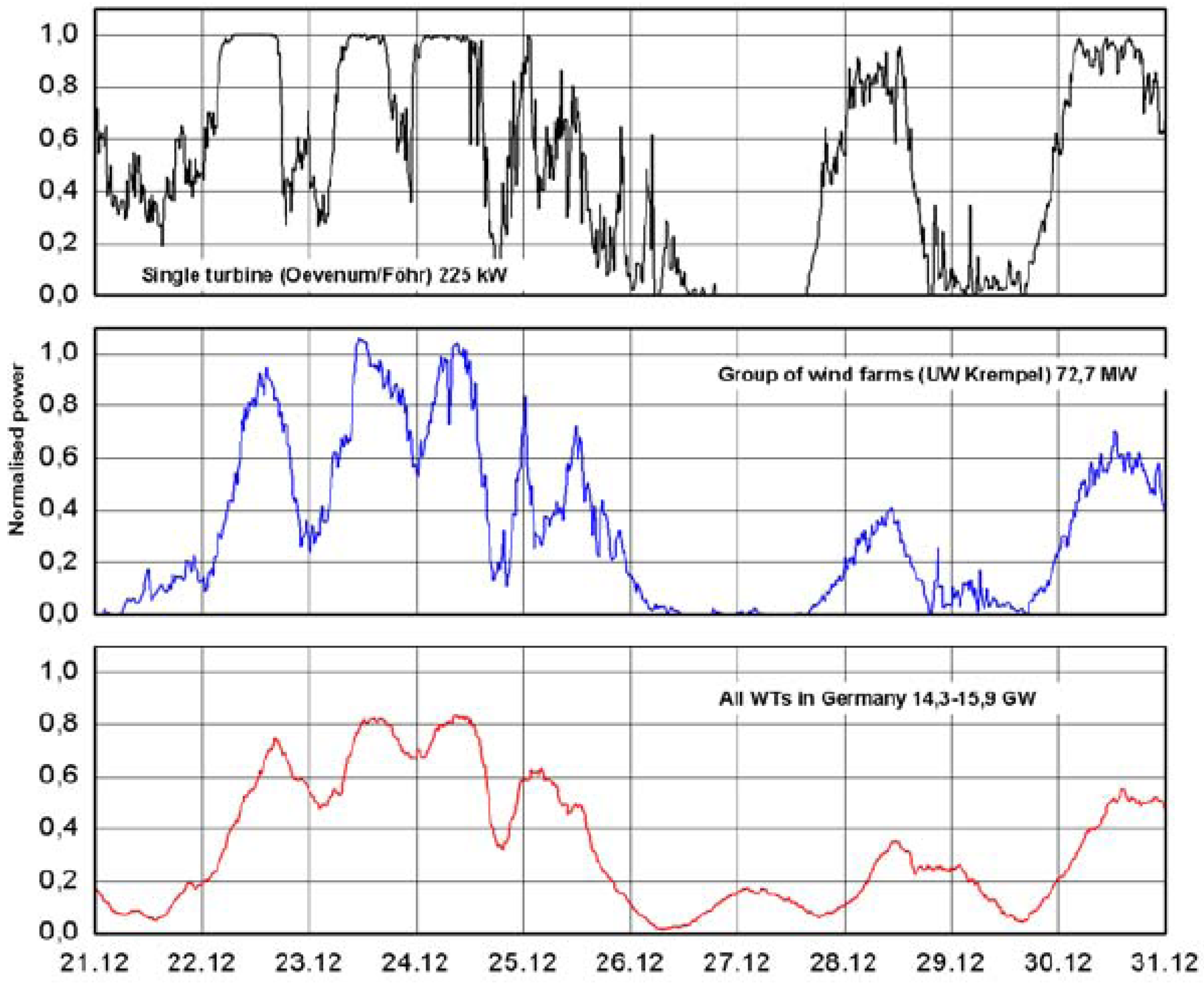
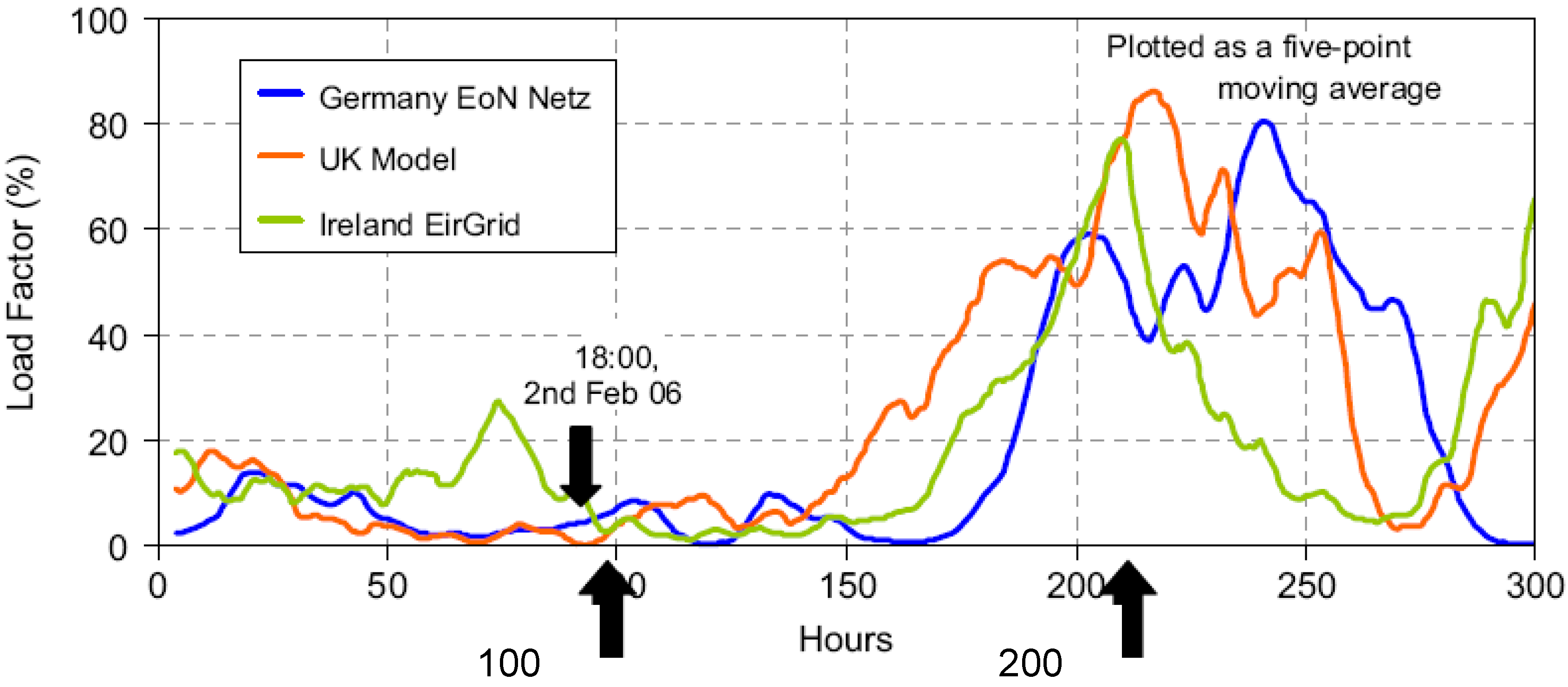
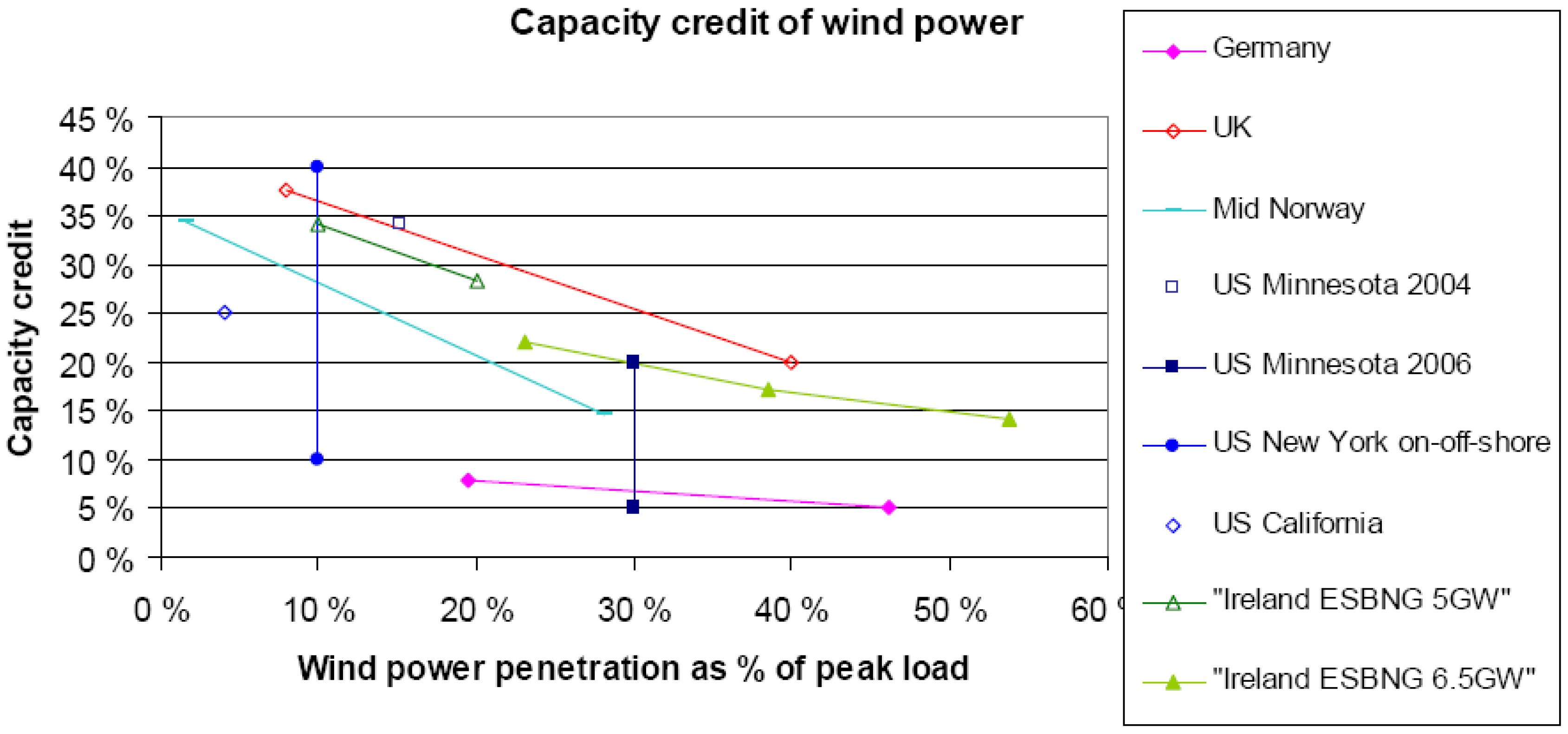
7.3.2. Capacity and load characteristics

Wind energy converters are dependent on the wind, and hence turbine output varies over time, at all time scales ranging from seconds to up to years. Measuring, modeling and understanding this variability is crucial for site selection, and also for integration of wind power into electricity grids.

In 2008, the global capacity of wind energy converters was 121 GW, generating about 260 TWh of electricity [51]. This yields a capacity factor of about 24.5% (Figure 44). Plant outages are not as problematic with wind power as they are with fossil, nuclear or large hydro, because numerous wind plants are usually distributed over a wide geographical area [207]. Such decentralization in a power supply system reduces the requirements for contingency reserve, since this type of reserve is mostly tied to the largest potential source of failure, that is the largest single generator in the system [208].

Figure 44. Average capacity factor as a function of wind speed. Most turbines operate in a range between 2000 and 3000 full load hours, which is equivalent to capacity factors between 23% and 34% (© 2004 Elsevier, reproduced with permission from [198]). For wind farms at certain windy sites, average capacity factors of up to 45% are reported [207].

Output from wind farms can be expected to be smoother than that of a single turbine, but smoothing effects on larger scales may not be so significant, and also vary between regions. Whilst smoothing effects are discernible when comparing single turbines with wind farms and regions (Figure 45, and also a similar figure for the UK in [209]), combining regions as such may not necessarily lead to much additional smoothing because of strong correlations in the wind regime over large distances (Figure 46).

Østergaard [193] artificially combines the wind output of West and East Denmark (which are not connected into a common grid) and obtains only small averaging effects. Oswald et al. [209] uses weather maps to demonstrate the correlation and variability of wind regimes across a large area combining Ireland, the UK and Germany (Figure 46). His findings (confirmed for Germany in [210], Section 3.1 and Figure 4) cast doubt on the effectiveness of a trans-channel “supergrid” in smoothing out variations in wind load. Holttinen et al. [211] present a detailed account of variability across geographical and temporal scales. Archer et al. [212] present wind speed data for a single site, and three and eight sites in Kansas, USA, and show how the frequency of low-wind events decreases as the number of included sites increases.

However, wind generators cannot—without storage—react to changes in demand because unlike hydro they cannot follow a fluctuating demand (Figure 47). Therefore, in the absence of supply-matched end-uses, they require a flexible electricity grid with a sufficient portion of technologies that can react quickly to demand changes, such as hydropower or natural-gas fired fossil plants [196,213].

Figure 45. Normalised power output from a single wind turbine (top), an group of turbines (middle), and al turbines in Germany (bottom; after [211]). © 2007 VTT, reproduced with permission from VTT Working Papers 82.

Figure 46. Variability and correlation of wind loads across Ireland, the UK and Germany. On 2 February 2006 the electricity demand in Britain reached its peak for 2006. © 2008 Elsevier, reproduced with permission from [209].

Figure 47. Wind power output and load in West Denmark (after [214]).

The average capacity factor of 24.5% given above does not reflect the circumstance that electricity system planners must meet demand whenever it occurs and not on average. Where a technology is assessed with regard to its ability to supply peak load, the capacity credit (Pavlak [215] calls this demand capacity) describes the fraction of average capacity that is reliably available during peak demand. The difference between the average capacity and capacity credit is proportional to the time when wind power cannot meet (peak) demand because of a lack of wind. For example, provided a filled reservoir, the capacity credit of hydro power is virtually equal to its average capacity, but this is not the case for wind power because of its variability and uncertainty. Some generators assign zero capacity credit to wind, however this is unrealistic [216]. Wind can achieve up to 40% capacity credit when penetration is low and times of ample wind coincide with times of high demand [217]. In general however, the higher the penetration of wind power in a power system, and the more uncorrelated wind output with demand load, the lower its capacity credit (see Figure 11 in [218], and Figure 48).

Capacity credit is usually measured by applying probability calculus to hourly data on load, generation capacity, ramp rates, and planned or forced outages, and applying merit orders in which technologies that avoid fuel costs are recruited first [220]. The Loss-Of-Load-Probability LOLP_i = Prob(∑_j C_j < L_i) (where C_j is the capacity of generator j in the grid, L_i is the load at hour i) is the probability that a supply system is not able to meet demand in hour i. Integrating LOLP over all operating hours results in the Loss-Of-Load Expectation LOLE = ∑_i LOLP_i, which is expressed in units of hours/year, or days/10 years, and provides a measure of system reliability. A common system LOLE target is 1 day / 10 years (this corresponds to a 1 – 1/(10×365) = 99.97% probability that the system will be able to meet demand without having to import capacity), in which case the system has to import capacity from elsewhere. A power supply system is usually made up of a technology mix. A measure that allows characterizing the incremental contribution of any one component to the reliability of the system is the Effective Load Carrying Capability ELCC, which is the new firm (i.e., zero-variance) load that can be added to the system including the incremental capacity increase, without deteriorating the system’s reliability. Adding a new generator G as well as a hypothetical firm load ELCC to a system, hourly LOLP becomes LOLP_i = Prob(∑_j C_j + G < L_i + ELCC). ELCC is a hypothetical firm (i.e., zero-variance) load that can be added to a system as a result of the addition of a non-firm (i.e., variable) capacity G, that would not change the system’s LOLE. ELCC is hence calculated by solving ∑_i Prob(∑_j C_j < L_i) = ∑_i Prob(∑_j C_j + G < L_i + ELCC). ELCC depends critically on the ability of a generator to meet demand at top-ranking LOLP hours, which, in the case of wind, is determined by the correlation of wind output with top-ranking LOLP hours. Capacity credit is the ratio of ELCC and rated capacity. Defined as such, capacity credit values are around or lower than average capacity (Figure 49). However, capacity credit has at times been measured as the ratio of ELCC and average power [219], in which case it varies between 0% and 100%. As a result, where grid operators are required to meet demand at usual loss-of-load expectations, reserve load-carrying capacity or storage has to be secured ([215]; Figure 49).

Operators also strive to avoid having to curtail surplus wind power at times of high wind, raising different management issues again [204]. Geographical dispersion of wind turbines can help reduce variability as well as increase predictability of output [208]. Even during a rapidly passing storm front, power from dispersed capacity will take a few hours to change [214]. Depending on the characteristics of the power system, that is composition and diversity of technologies, demand management, size, demand profile, and the degree of interconnection, low capacity credit poses barriers to the degree of integration of wind energy. In general, the more flexible, load-following capacity there is in the existing grid, the higher the potential penetration of wind power. However, operators run either the risk of not meeting demand by committing too much cheap slow-start capacity, or the risk of overrunning cost by committing too much expensive fast-start capacity [221].

Figure 48. Capacity credit of wind power as a function of wind penetration (reproduced with permission from [217]). Note that as penetration approaches 20%, the capacity credit starts to fall consistently below wind power’s average capacity factor. The results from Mid-Norway show that geographical dispersion improves capacity credit. Decreasing capacity credits have been confirmed theoretically for a while, for example by [219].

Figure 49. Typology of grid impacts of wind power across temporal and spatial scales (© 2008 IOP, reproduced with permission from [204]). Balancing reserves deal with short-term variability in the order of up to 24 h. Adequacy in peak-load situations (i.e., low LOLE) has to be secured long-term and requires load-carrying reserves to compensate for shortfalls in capacity credit.

Grid integration issues have largely been studied theoretically, except for some European regions. For example, whilst Denmark receives on average more than 20% of its electricity from wind, it sometimes receives much higher percentages, and sometimes very little, in which case Denmark exports or imports electricity from the European grid, and thus relies on other generation technology for load balancing [215,222], in particular Norwegian, Swedish and Finnish hydro reservoirs, and idle peaking plants in Denmark [223]. For higher degrees of integration, the management and/or export of excess wind loads becomes an issue [221]. Söder et al. [214] report results from four regional systems with high wind penetration, amongst which two are connected to a larger outside system, and two are not. Management of wind power variability involves the requirement for flexible interconnection capacity, and the ability to curtail wind power production, respectively. Hoogwijk et al. [191] (their Figure 9) find that—subject to supply and load correlation—the amount of electricity that has to be discarded grows strongly for penetrations in excess of 20%–30%. Lund [224] investigates a scenario for expansion of wind power to cover 50% of Danish demand, and concludes that supply-demand balancing problems would become severe. Similarly, penetration of less than 20% can lead to instabilities if a grid is not well interconnected with other grids, such as in the case of Spain [191].

7.3.3. Life-cycle characteristics

Lenzen and Munksgaard [52] review and analyse a large body of literature on the life cycle of wind energy converters, comparing bottom-up component analyses with top-down input-output analyses. In their multiple regression these authors take into account technical features such as scale, vintage year and load factor, but also scope and methodology of the analysis (Figure 50).

A more recent study by Wagner and Pick [225] confirms the energy pay-back times between 3 and 7 months, which—assuming a turbine lifetime of 20 years—corresponds to cumulative energy requirements between 0.035 and 0.075 kWh_th/kWh_el. The cumulative energy requirement η is related to the energy payback time, that is the time it takes the wind turbine (life time T) to generate the primary-energy equivalent of its energy requirement, via t_payback = η · T · ε_fossil. ε_fossil is the conversion efficiency (assumed to be 35%) of conventional power plants that are to be displaced by WTs. Lenzen and Munksgaard [52] found greenhouse gas intensities for the larger, modern turbines to be about 10 g/kWh_el, ranging amongst the lowest values for all electricity generation technologies.

Roth et al. [53] and Pehnt et al. [226] take the reduced capacity credit of wind into account in their systems’ LCA, and conclude that CO₂ emissions arising from the need of additional reserves add between 35 and 75 g CO₂/kWh, thus outweighing CO₂ emissions from the turbine life cycle. However, these values depend strongly on the technology mix of the overall power system.

Figure 50. Cumulative energy requirements of wind energy converters as a function of rated power. The multivariate regression line takes into account different scopes and methodologies adopted in case studies. A ratio of thermal energy input to electricity output of 0.05 kWh_th/kWh_el is found to be realistic for modern large turbines. © 2002 Elsevier, reproduced with permission from [52].

Noise, and impacts on birds is likely to be small from wind farms, compared to other impact causes [196]. Snyder and Kaiser [203] provide a detailed account of possible ecological impacts from off-shore wind farms. The mitigation potential of wind in a power system represents an optimisation problem, because the higher the penetration of wind power, the higher emission reductions, but also the higher the variability cost (see Section 6.3.6).

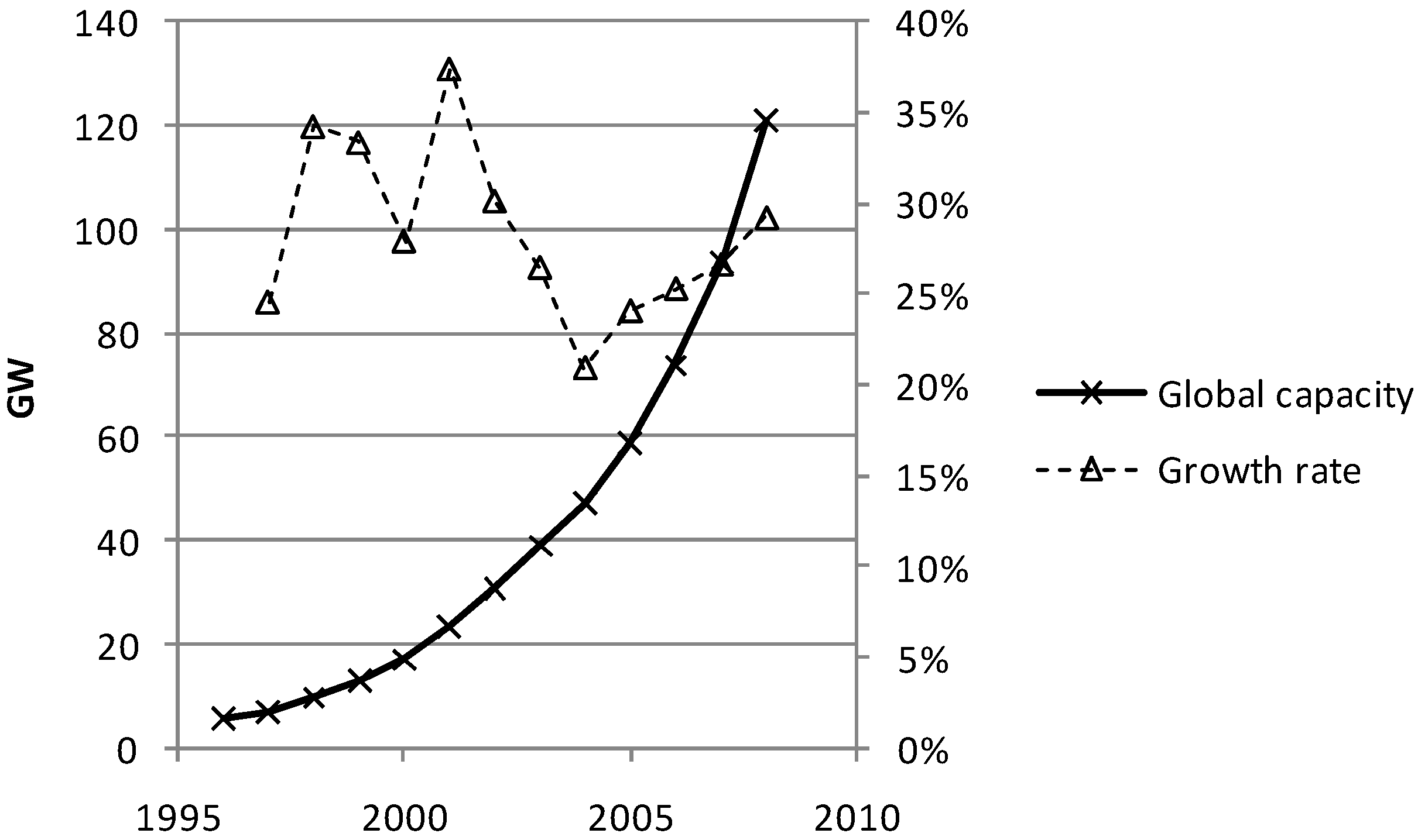
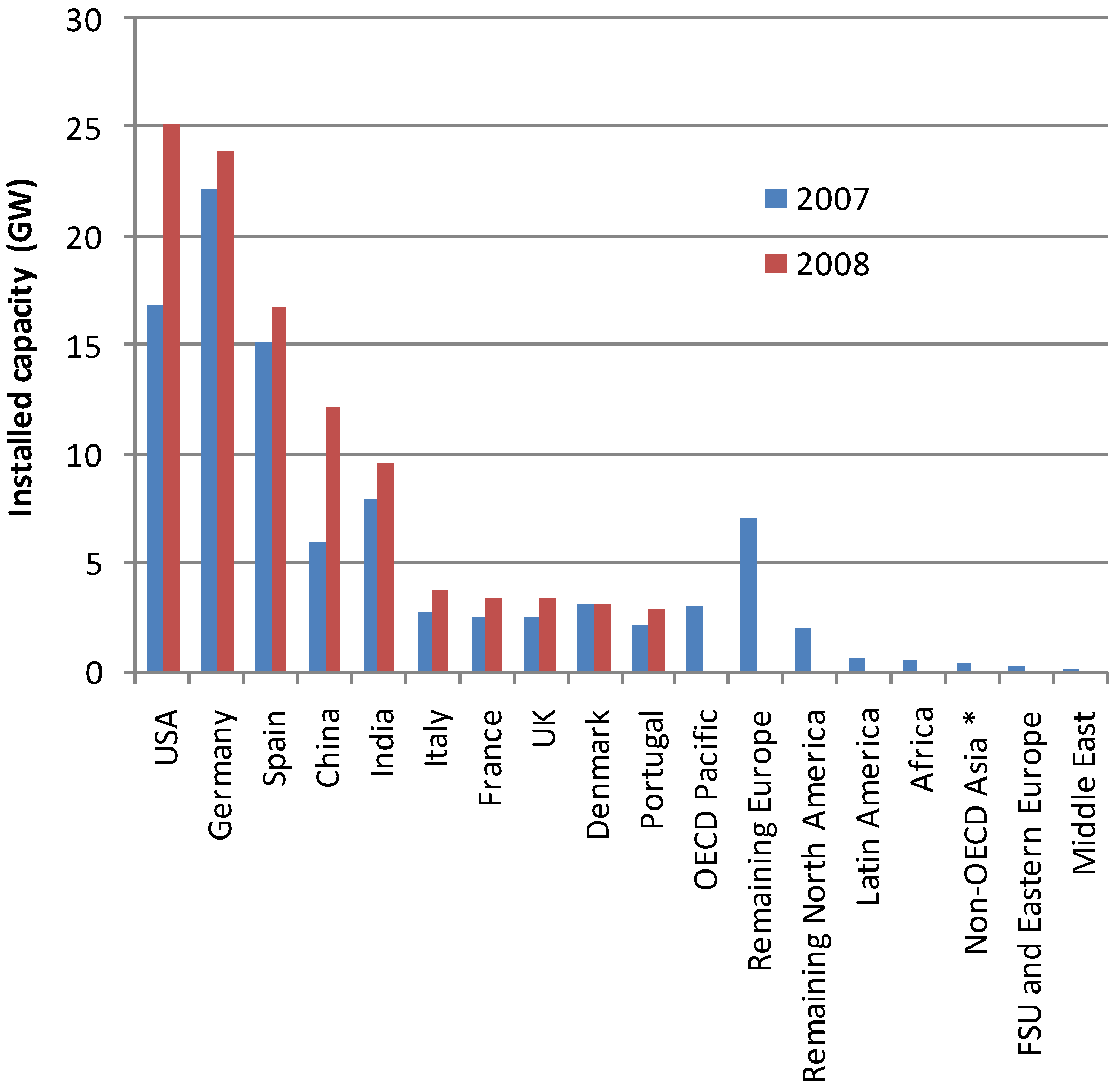
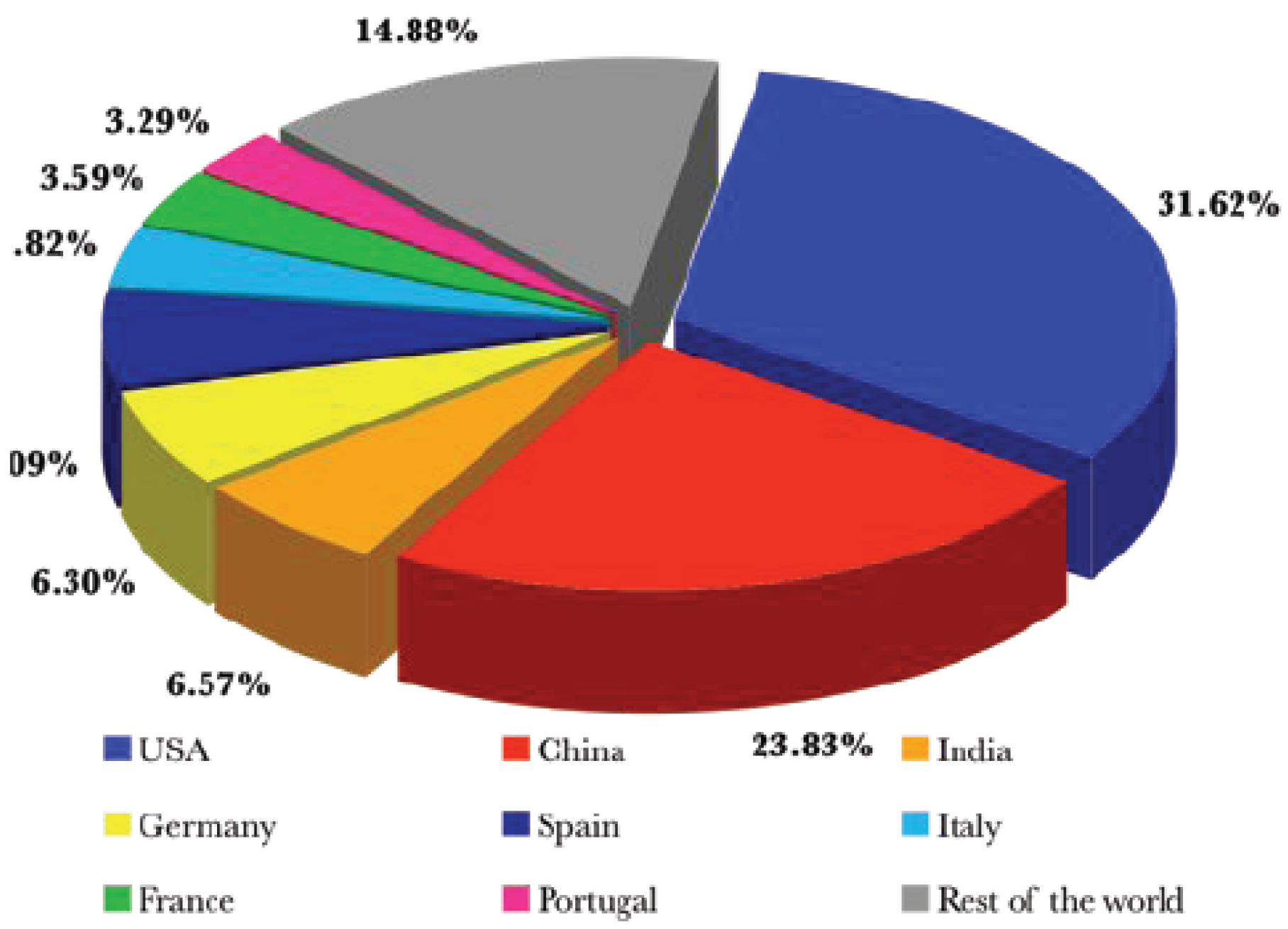
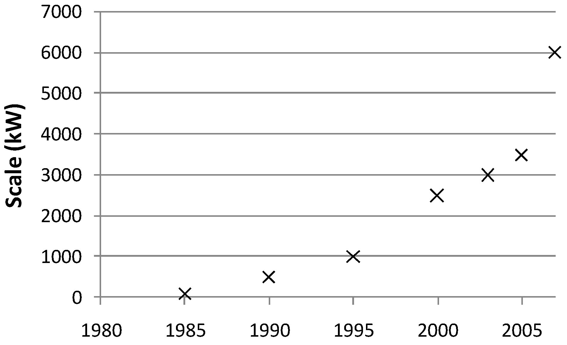
7.3.4. Current scale of deployment

Due to large economies of scale the scale of single wind energy converters has been increasing steadily (Figure 51), featuring taller towers and larger rotors.

Larger turbines with ratings above 3.5 MW are usually dedicated to off-shore power generation, while on-shore installations have been largely between 1.5 and 3 MW [196]. In early 2009, the French manufacturer Areva deployed 5 MW turbines for operation 45 km offshore of the German North Sea island of Borkum [227]. 5 MW turbines are also installed at the Beatrice site (40 m depth) off the Moray Forth east of Scotland (http://www.repower.de/index.php?id=369). In 2007, the average size of operating turbines was 1.5 MW.

Figure 51. Maximum scale of wind energy converters over time (compiled after [228], [198] and [196]).

7.3.5. Contribution to global electricity supply

In 2008, the global capacity of wind energy converters was 121 GW, generating about 260 TWh of electricity, or about 1.5% of global electricity production [51]. Most of the capacity (Figure 40) is installed in the USA (25 GW, 1% of electricity generation) and in the EC (about 65 GW, 3.7%), followed by China (12 GW) and India (10 GW). Regional shares of wind power are much higher in some countries, such as Denmark (21%), Spain (12%), Portugal (9%), Ireland (8%), and Germany (7%). However note that Denmark at times receives much higher percentages of its electricity from wind, and sometimes very little, in which case Denmark exports or imports electricity from the European grid, and thus relies on other generation technology for load balancing [215].

Wind energy deployment has been increasing rapidly throughout the past decade, recording growth rates of around 30% since 1996 (Figure 41). More than half of the 2008 additions occurred in the USA and in China (Figure 42), with the USA overtaking Germany as the leader in installed wind capacity [51]. In the USA, wind power has represented 40% of 2007 national capacity growth [229]. Most of wind generation is on-shore; only about 1.1 GW is presently installed off-shore, mainly located in Denmark (420 MW), the UK (300 MW), Sweden (135 MW), and the Netherlands (130 MW) [230] (www.ieawind.org/Annex_XXIII.html). A further 8 GW were planned in early 2009 [227].

7.3.6. Cost of electricity output

Capital costs make up about 80% of total wind energy cost, with the remainder for operation and maintenance, since the wind turbine does not require any fuel input. Blanco [231] presents a detailed breakdown of these costs; in on-shore installations, the turbine covers 70% of capital cost, with the remainder for grid connection, civil works, taxes, permits, etc. Within the turbine, the tower and blades make up for half of the costs. Electricity costs vary with site conditions: Assuming a 20-year plant life, 5–10% discount rate, and 23% average capacity factor, Blanco [231] states a levelised cost range for power from European 2 MW wind turbines between 6.5 and 13 US¢/kWh. Welch and Venkateswaran [232] and Snyder and Kaiser [203] report US cost estimate between 3 and 5 US¢/kWh, whereas DeCarolis and Keith [221] reported between 4 and 6 US¢/kWh. Civil works, and especially the foundations are much more expensive in off-shore installations, where they represent 20% of capital cost, leading to higher levelised cost of 9–16 US¢/kWh. This is confirmed in an estimate of 10 US¢/kWh by Snyder and Kaiser [203]. However, technological learning can bring these costs down in the future [230,233].

Wind energy costs have increased during the past three years, mainly driven by supply tightness and price hikes of raw materials [230], which is difficult to control by government fiscal policy. Bolinger and Wiser [229] provide a detailed analysis of most recent upward cost trends. Yet, the analysis of learning curves for the industry suggests that levelised costs will come down through increased efficiency, by about 10% for every doubling of capacity ([231], compare Figure 14 in [1]). As with other non-fossil electricity generation technologies, wind plant operators expect the competitive landscape to change in favour of wind power, once carbon is adequately priced [196,221]. In the future, wind energy is also expected to benefit more from not being affected by fuel price risks.

However, depending on the penetration of a power system with variable wind energy, additional indirect cost arise for maintaining LOLE, because wind energy will not be able to meet demand at its average capacity factor, but at a generally reduced rate depending on its capacity credit [221]. In addition, the presence of wind power in a power supply system introduces short-term variability and uncertainty, and therefore requires balancing reserve scheduling and unit commitment. Grid operators need to meet peak demand to certain statistical reliability standards even when wind output falls relative to load. During these periods, which range from minutes to hours, electricity markets need to recruit demand-following units (such as gas, hydro, or storage), which at times of sufficient wind remain idle, so that costs arise essentially for two redundant systems [215,234], and for inefficient fuel use during frequent ramping (see p. 903 in [235], and [191,234]). Both adequacy and balancing cost (compare Figure 49) are sometimes referred to as intermittency cost, however in this report the term variability cost will be used because strictly speaking wind energy is variable and not intermittent [216]. Thus, wind energy reduces dependence on fuel inputs, but does not eliminate the dependence on short-term balancing capacity and long-term reliable load-carrying capacity.

The impact of wind power on the power supply system is critically dependent on the technology mix in the remainder of the system, because the more flexible and load-following existing technology, the less peak reserves are needed. It is also dependent on time characteristics of system procedures (frequency of forecasts etc) and local market rules [204]. In general, the higher the wind penetration, the higher the variability in the supply system, and the more long-term reserve and short-term balancing capacity has to be committed (Figure 52 on short-term balancing only).

The corresponding cost increases are only partly offset by a smoothing out of wind variability when many turbines are dispersed and interconnected over a wide geographical area [236], but they are more than offset by reduced fuel and operating cost. In specific applications, the cost of additional wind power also depends on the relative locations of turbines, load, and existing transmission lines, and on whether sufficient load-carrying reserve exists in the grid or has to be built. As expected, variability costs scatter significantly depending on a large array of parameters. They cannot be derived from capacity credit estimates, since these do not contain any information about to what extent cheap base load and expensive peak load are being displaced by wind [237]. Variability costs are difficult to disentangle from overall cost in real-world grids [221], so that they have largely been estimated for theoretical settings, using statistical models for resource and load fluctuations, and least-cost-optimising generation and reserve scheduling under given output limits, startup and shutdown cost, ramp-rate restrictions, planned outages, fuel cost, and day-ahead forecasts [208,236]. They have been quoted between 0.2–0.4 US¢/kWh for existing installations [196,203], but also higher at 1–1.8 US¢/kWh [221,234,238] for larger degrees of wind penetration. In a more up-to-date survey, Holttinen [204], Strbac et al. [218] and Smith et al. [235] report on recent findings about increases in balancing requirements due to the presence of wind, ranging widely between 0.05 and 0.5 US¢/kWh (Figure 53). Hence, at penetrations of up to 20%, variability cost can be expected to be about equal or less than 10% of generation cost.

Hoogwijk et al. [191] (see Figure 54) ran numerical experiments at large-scale penetration rates of up to 45%, and find that beyond 30% penetration the cost incurred by discarded excess electricity becomes comparable to base cost (6 US¢/kWh).

The market for wind turbine manufacturing is diverse and competitive, with manufacturers spread across many countries. However, large corporations are entering the market, sometimes assimilating smaller entities [196]. During the recent wind market boom, and the shift to larger turbines, the industry faced a number of supply chain bottlenecks related to gearboxes and large bearings [231], leading to waiting times for turbines of up to 30 months [223].

7.3.7. Technical challenges

The variable and distributed nature of wind energy requires specific grid infrastructure in order to ensure grid stability, congestion management and transmission efficiency. Significant investment in grid infrastructure has to occur in order to allow for substantial global penetration of wind energy [196]. One of the most significant challenges is hence the integration of wind power into a large grid, and the theoretical modeling of power system behaviour at high penetration rates of wind. Recent efforts are also aimed at improving short-term forecasting of wind, which is still less accurate than forecasting of load [211]. With increasing interconnection and geographical dispersion, forecasting errors are expected to decrease (see Figure 55).

Figure 55. Measured forecast error as a function of spatial range of interconnection (© 2007 VTT, reproduced with permission from VTT Working Papers 82 [211]). The error reduction plotted on the y-axis is the ratio of the root-mean-square error (rmse) of prediction at a regional scale, and the single-site prediction rmse.

Some researchers suggest directing wind power to where it can be most competitive, or where its variability does not create problems. Some industrial applications and also combined heat and power plants can—within limits—adjust their demand to supply [222]. Dedicated load-leveling applications such as desalination, aluminium smelting, space and water heating, or a chargeable hybrid vehicle fleet can deal with hourly variations in wind power since they only require a certain amount of energy over a period of many hours [202,215]. For example, large-scale vehicle-to-grid technology can significantly reduce excess wind power at large wind penetration and replace a significant fraction of regulating capacity, but as Lund and Kempton [239] shows in a study for Denmark, electric vehicles would not nearly eliminate excess power and CO₂ emissions, even if they had long-range battery storage.

Tavner [240] and Smith et al. [235] list improvements in resource, turbine and systems modelling and forecasting, capital cost reduction, lifetime extension, transmission upgrading, and system integration as the main future research challenges for wind power. Joselin Herbert et al. [228] reviews past developments and present research needs for wind technologies, such as for resource assessment, site selection, turbine aerodynamics, wake effects, and turbine reliability. Off-shore wind deployment faces technical challenges in form of extreme wind conditions that exceed tolerances of current on-shore turbines [203,233]. The IAE Wind off-shore subgroup’s tasks include research on ecological issues and deep-water installation. In order to reduce off-shore wind costs, turbine concepts, submerged structures and cabling, and remote O&M will need to undergo further research [231]. Many of the above issues are approached though theoretical modeling, be it turbine structure, system control and balancing, wind conditions, or reliability [240]. Surprisingly, offshore wind shares many of large hydro and nuclear’s challenges regarding public opinion. Firestone and Kempton [16] report from a case study where the majority of survey respondents opposed offshore wind power development for environmental reasons, and that many of the beliefs were “stunningly at odds” with the scientific literature. Perceived landscape changes also feature in a survey by Zoellner et al. [241], but economic considerations more strongly influenced acceptance.

8. Photovoltaic power

8.1. Summary

The International Energy Agency’s Photovoltaic Power Systems Programme (IEA-PVPS; www.iea-pvps.org) coordinates information exchange between member countries and research & development related to PV power. The IEA-PVPS also collects and publishes PV-related statistics. Because of the numerous dispersed and small-scale applications, statistics on PV deployment can be incomplete. For example, many of the figures given in this Section apply to IEA-PVPS member countries only.

Currently, 9 GW of PV technology are predominantly deployed as grid-connected crystalline silicon modules, with efficiencies of up to 20%. The average capacity factor of PV power is comparatively low at 15%, but especially in sunny locations with high mid-day peak loads for example for air conditioning, PV’s capacity credit can be up to 80%. Life-cycle greenhouse gas emissions are comparatively high at 100 g CO₂/kWh. The main present obstacle and future challenge for larger deployment of PV technologies are the high electricity generating cost; even under favourable conditions they are above 10 US¢/kWh. Whether PV will achieve cost parity with current technologies, and represent a significant portion of future electricity supply, will depend critically on future technological learning aimed at reducing generating costs.

8.2. Global potential of resource

Whilst the theoretical potential of PV power is in excess of global energy demand [242], the economic potential is currently small because of the comparatively high cost of PV-generated electricity. As a consequence, PV currently deploys only about 9 GW world-wide, which is mostly grid-connected, and significantly subsidised. PV power is currently only economical in remote settings where users are not connected to an electricity grid. Under these niche conditions however, PV has been quite successful worldwide.

PV power has a higher capacity credit than wind power, especially in sunny and hot locations where there are large summer mid-day loads from air conditioning. However, in order to be scaled up to beyond 10% of global electricity production, PV may have to be deployed in desert areas [195,242,243,244] in connection with either High-Voltage DC transmission or liquid hydrogen production and transport facilities [195,245], in order to deal with the large distances between unused and sunny areas, and densely populated areas with high power loads

The long-term future potential of PV is uncertain, and is mainly determined by whether cost can be lower sufficiently to be competitive with other generation technologies. The break-even of PV depends critically on the assumed learning ratio. Van der Zwaan and Rabl [55] analyse technological learning of PV between 1976 and 1996, and conclude a learning rate of 20% (or a progress ratio of 0.8, see their Figure 2; compare with [144], and Figure 14 in [1]). However, based on more recent data in [246] and [247], learning rates between 1997 and 2007 have decreased to 10% (progress ratio of 0.9). Interestingly, at progress rates of 0.8, PV can attain break-even at a cumulative deployment of 148 GW (compared to present 9GW), subject to a cost-gap funding of 64US$b, or 37 US$b after subtracting externality avoidance (see Table 7, compare with the estimate of US$300b in Section 4.1 of [248], and with [249]). However, at current progress rates around 0.9, breakeven cumulative production is larger than global power plant deployment, and hence PV would never break even under these conditions, even imposing damage cost on other technologies.

Table 7. Breakeven conditions for PV power under varying progress ratios (© 2004 Elsevier, reproduced with permission from [55]). 2^nd and 3^rd rows: cumulative production needed to achieve break-even; 4^th row: integral under the learning curve; 5^th row: cost of producing breakeven deployment under breakeven conditions; 6^th and 7^th rows: breakeven cost gap; 8^th and 9^th rows: avoided externality cost, to be compared with cost gap.

**Table 7.** Breakeven conditions for PV power under varying progress ratios (© 2004 Elsevier, reproduced with permission from [55]). 2^nd and 3^rd rows: cumulative production needed to achieve break-even; 4^th row: integral under the learning curve; 5^th row: cost of producing breakeven deployment under breakeven conditions; 6^th and 7^th rows: breakeven cost gap; 8^th and 9^th rows: avoided externality cost, to be compared with cost gap.
Progress ratio, pr	0.7	0.75	0.8	0.85	0.9
Breakeven cumulative production, n_b (GW_P)	23	48	148	957	39700
Breakeven cumulative production, as % of 3300 GW, the present world capacity	0.7%	1.5%	4.5%	29.0%	1200%
Cost of reaching breakeven, C_b ($ billion)	37	74	211	1240	46800
Cost of producing n_b – n₀, if unit cost were already at breakeven, (n_b – n₀) c_b ($ billion)	22	47	147	956	39700
Cost gap, C_b – (n_b – n₀) c_b ($ billion)	15	27	64	288	7110
Cost gap (% of cost of reaching breakeven)	41%	36%	30%	23%	15%
Avoided damage of n_b – n₀ (at 0.25 $/W_P, in $ billion)	5	12	37	239	9920
Avoided damage (% of cost gap)	37%	44%	58%	83%	140%

Source: authors’ calculations. Assumptions: current cumulative production n₀ = 1 GW_P, current unit cost c₀ = 5 $/W_P, breakeven unit cost c_b = 1.0 $/W_P.

Similarly, it is very difficult to estimate PV’s greenhouse gas mitigation potential, because of the uncertainty in cost. The technological potential is much higher than current global electricity demand, however the realisable economic potential depends critically on learning curves and future cost (Figure 56).

PV power (based on both crystalline and thin film technologies) is not expected to be competitive before 2020 [55,248]. Extrapolating past learning curves, growth rates and economies of scale, Hoffmann [250] envisages PV’s share in global electricity generation to pass the 1% mark around 2030, which implies growth rates to decline to about 20% per year. Such growth rates are at the lower limit of what EPIA [246] projects until 2012.

In various scenarios, Resch et al. [205] estimate 2030 potentials between 1.5% and 4.5% of global generation, which agrees roughly with the ACT and BLUE scenarios of the IEA [2] projecting 2050 potentials between 3% and 5.5%. Raugei and Frankl [249] cite a pessimistic scenario of 2% in 2050, a “realistic scenario” where 2025 deployment is 55 GW, and 2040 deployment is 2400 GW, and an optimistic scenario with 9000 GW in 2050. Fthenakis et al. [248] project US PV deployment at 130 GW in 2030, 1450 GW in 2050, and 6000 GW in 2100. The wide range of just the few projections above means that PV’s mitigation potential could be anywhere between 25 and 200 Gt CO₂.

Figure 56. Technical potential of PV as a function of generation cost [191]. The realisable economic potential is critically dependent on how much generation cost can be lowered to achieve cost parity (including externalities). © 2007 Elsevier, reproduced with permission.

8.3. Photovoltaic cells, modules and systems

8.3.1. Technical principle

The basic component of a PV power system is the photovoltaic or solar cell. The cell is encapsulated and wired in a so-called PV module, which is commercially sold. Modules are mounted on rooftops, posts or other structures, sometimes in solar arrays. In grid-connected applications, an inverter is needed to transform the cell’s DC output into AC. Off-grid applications can work with DC, but need a storage system (for example a battery) and a charge controller [251].

There are a number of cell types that are distinguished by their material properties. Crystalline silicon cells are produced from melting of PV grade silicon; these account for the majority of PV production and applications (Figure 57). Single-crystal PV cells are produced by growing a single crystal, whilst multicrystalline cells are manufactured in a melting and solidification process. Multicrystalline cells are less expensive than single-crystal cells, but because of the interfaces between the crystals, their commercial conversion efficiency is lower at around 14%, compared with 15%–18% of single-crystal cells. Cells are produced by sawing ingots or ribbons into wafers.

Since light is converted into electric charge only in a thin surface layer of the cell, one way of reducing cell costs are thin film cells. These are produced by deposition of PV semiconductor material (amorphous silicon, cadmium telluride CdTe, and copper-indium-gallium-arsenide compounds CIGS) onto a glass, plastic or metal substrate. Commercial thin film efficiencies are between 7% and 13% [251]. Laboratory technology has achieved much higher efficiencies of above 25% (single crystal) and 19% (thin film).

PV systems are classified according to their grid operation mode. Off-grid devices are not connected to a utility electricity network. Grid-connected distributed systems are often small systems installed on residential, public or commercial buildings, where they supply the user directly, and during periods of excess power feed into the electricity network. Grid-connected centralised systems operate as power stations that do not supply a particular user, but rather generate bulk power [251].

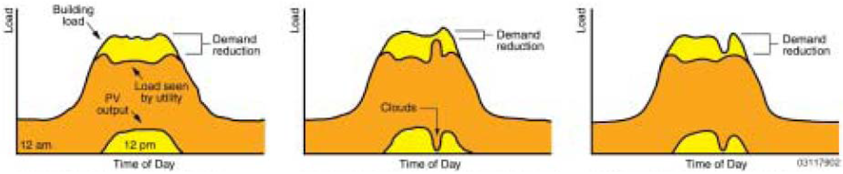
8.3.2. Capacity and load characteristics

It is difficult to ascertain an average capacity factor for the entire PV capacity, since most applications are small-scale and distributed amongst many individual consumers. Lenzen et al. [47] (Section 6.6.2) report average capacity factors between 5% and 15%. Large-scale power plants achieve average capacity factors around 15% [250].

In contrast to wind power, solar output is temporally correlated with certain segments of load, and hence the Effective Load-Carrying Capacity (ELCC) of solar PV is much higher than that of wind. Perez et al. [252] determine the ELCC for PV systems operating across the US, and derive ELCCs for tracking- and fixed-mode installations as a function of grid penetration and Summer-to-Winter Peak Ratio (SWPR). Their main results are that a) solar output is mainly correlated with typical summer loads such as air conditioning, so that ELCCs are high for locations where the summer peak load is higher than the winter peak load (SWPR > 1), and vice versa, and that b) ELCC decreases with increasing grid penetration (Figure 58).

Figure 58. ELCC as a function of grid penetration and SWPR for US 2-axis tracking PV systems (derived from [252]).

Figure 59. ELCC as a function of grid penetration and SWPR for US fixed 30°-angle south-facing PV systems (derived from [252]).

Once SWPR falls below 1, the capacity credit of PV systems decreases rapidly. However, even at high grid penetration of around 20% and SWPR of 0.8, solar power has more capacity credit than wind. Further, Perez et al. [252] find that PV systems installed at a fixed angle perform worse than tracking systems (Figure 59). On a national average basis, for a country such as the US with its diverse climates, and hence varying SWPRs, fixed PV systems achieve PV capacity credits of around 55% at low penetrations, decreasing to around 35% at 20% penetration. Rüther et al. [253] obtain similar results for the city of Florianópolis in Brazil. In Canada with a higher winter load, the ELCC is between 25% and 40% at low penetration, and between 15% and 25% at 20% penetration [254].

These results show that PV’s ability for providing dependable capacity is in locations with high and correlated (for example commercial day-time) summer peak loads, such as California, where it can reduce the number and run-time of fossil peak reserve plants [255].

Figure 60. Summer peak load (envelope of curve) and solar peak capacity (yellow) [255].

Herig [255] describes applications where local electricity demand can be adjusted to solar output, because the demand is correlated with insolation (Figure 60, left). Solar output will decrease temporarily when clouds obscure the sun, meaning that reserve capacity has to be mobilised (Figure 60, middle). However, if office air-conditioning systems are ramped down during periods of cloud cover (since air conditioning demand should be lower), using a Solar Load Controller (SLC, Figure 60, right), then peak reserves are not needed. Using such SLCs, the capacity credit of PV systems can locally approach 100%. As with wind power, solar power is well suited for demands that are insensitive to temporal variations in electricity output, such as water pumping for irrigation, or vehicle charging. Matching such loads with variable solar resources can overcome restrictions related to limited capacity credit.

8.3.3. Life-cycle characteristics

Lenzen et al. [47] undertake a review of LCA studies on PV systems. The main results of their review are that a) currently operating plants report much higher energy requirements and greenhouse gas emissions per kWh generated than conceptual designs, which is largely due to the small scale of production and operation, b). An input-output study by Crawford et al. [256] highlights the importance of an appropriate LCA method: These authors showed that 55% of the complete life-cycle inventory for building-integrated PV resided in indirect impacts that were outside the boundary of conventional assessments.

Table 8. Energy requirements and greenhouse gas emissions for a hypothetical 100-MW PV plant operating under Australian conditions. BOS = Balance Of System. © 2006 ISA, reproduced from [47] with permission.

**Table 8.** Energy requirements and greenhouse gas emissions for a hypothetical 100-MW PV plant operating under Australian conditions. BOS = Balance Of System. © 2006 ISA, reproduced from [47] with permission.

In a case study of a hypothetical 100-MW PV plant (crystalline silicon, module efficiency 13%, system efficiency 80%) operating under Australian conditions (average capacity factor 20%, and coal-based background economy), Lenzen et al. [47] (work undertaken by author Wood) arrive at specific energy requirements of 0.33 kWh_th/kWh_el, and specific greenhouse gas emissions of about 100 g CO₂/kWh_el (see details in Table 8).

Most LCA studies on operating and conceptual plants assess crystalline silicon technology. Where amorphous silicon technology is assessed, stated energy requirements and greenhouse gas emissions are lower than for crystalline silicon [47]. Further, specific energy requirements and greenhouse gas emissions depend critically on the system’s capacity factor. The IEA-PVPS [251] and Fthenakis and Kim [116] report life-cycle greenhouse gas emissions from PV systems in locations of high insolation of around 50 g/kWh. In less sunny locations such as across Europe, or in carbon-intensive economies these emissions can be up to 2–4 times higher. Finally, none of the above figures include emissions from fossil peak reserves that arise out of the variability of solar output. However, these emissions are likely to be lower than in the case of wind power, because PV’s capacity credit is significantly higher than that of wind.

In terms of environmental impacts other than greenhouse gas emissions, Fthenakis and Kim [257] find that CdTe PV technologies emit less cadmium throughout their life cycle than coal- and oil-fired power plants. In a dynamic LCA, Pehnt [30] projects future life-cycle impacts of PV to decrease by about 40% until 2030.

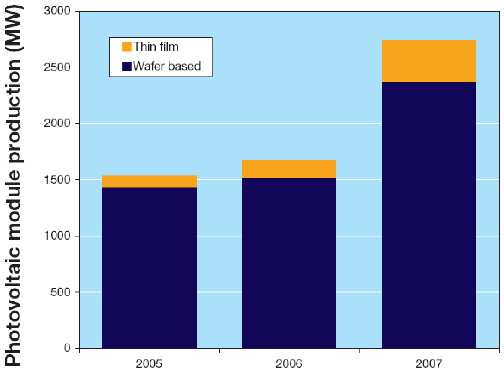
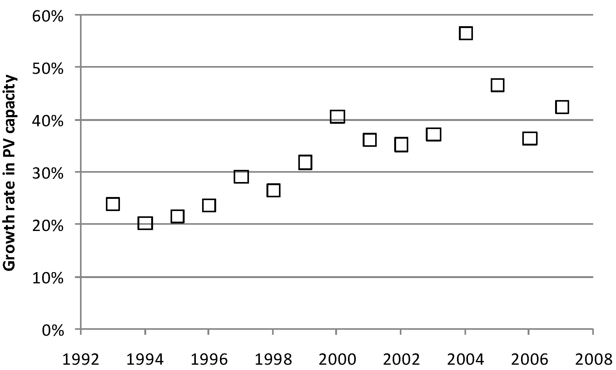
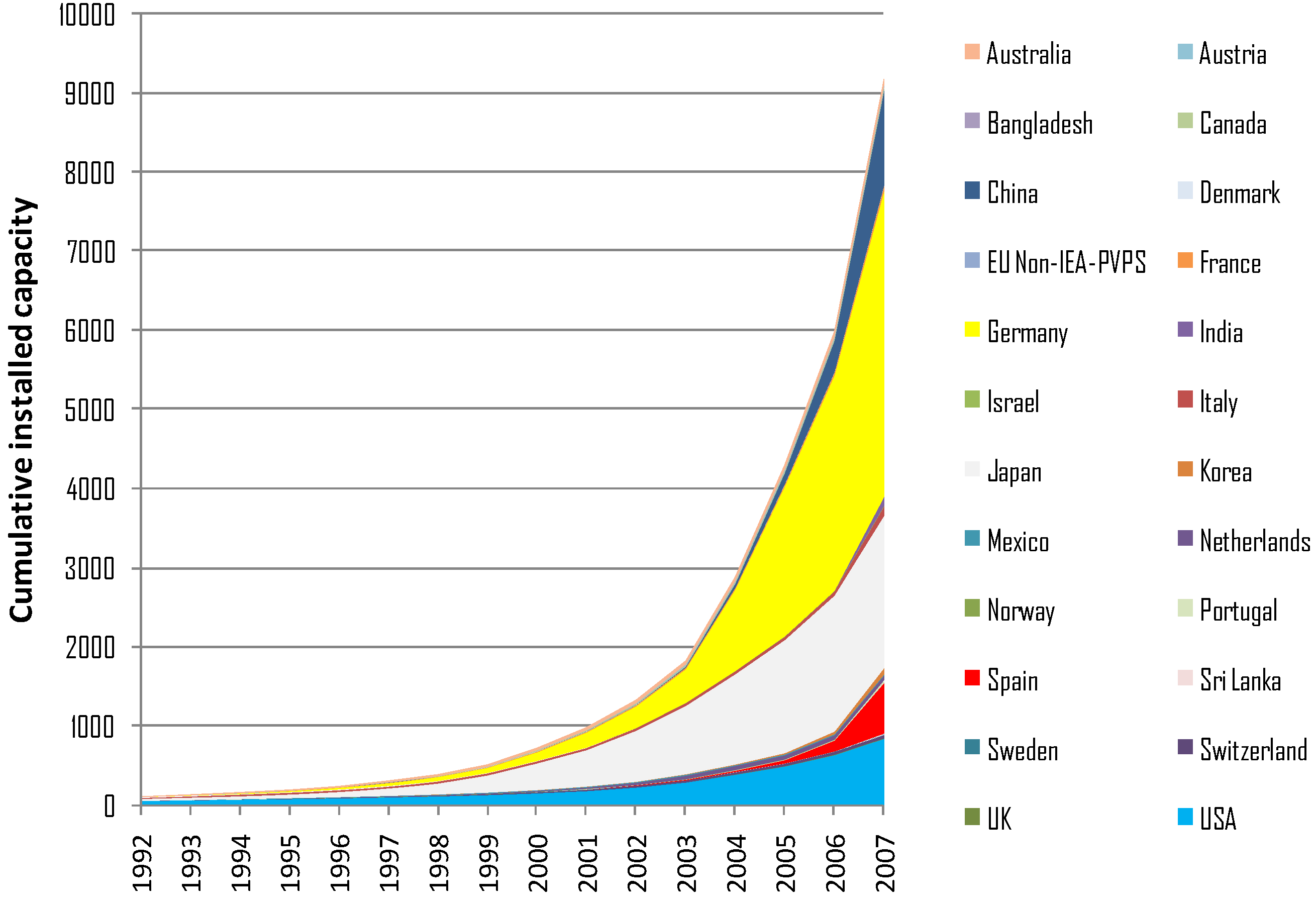
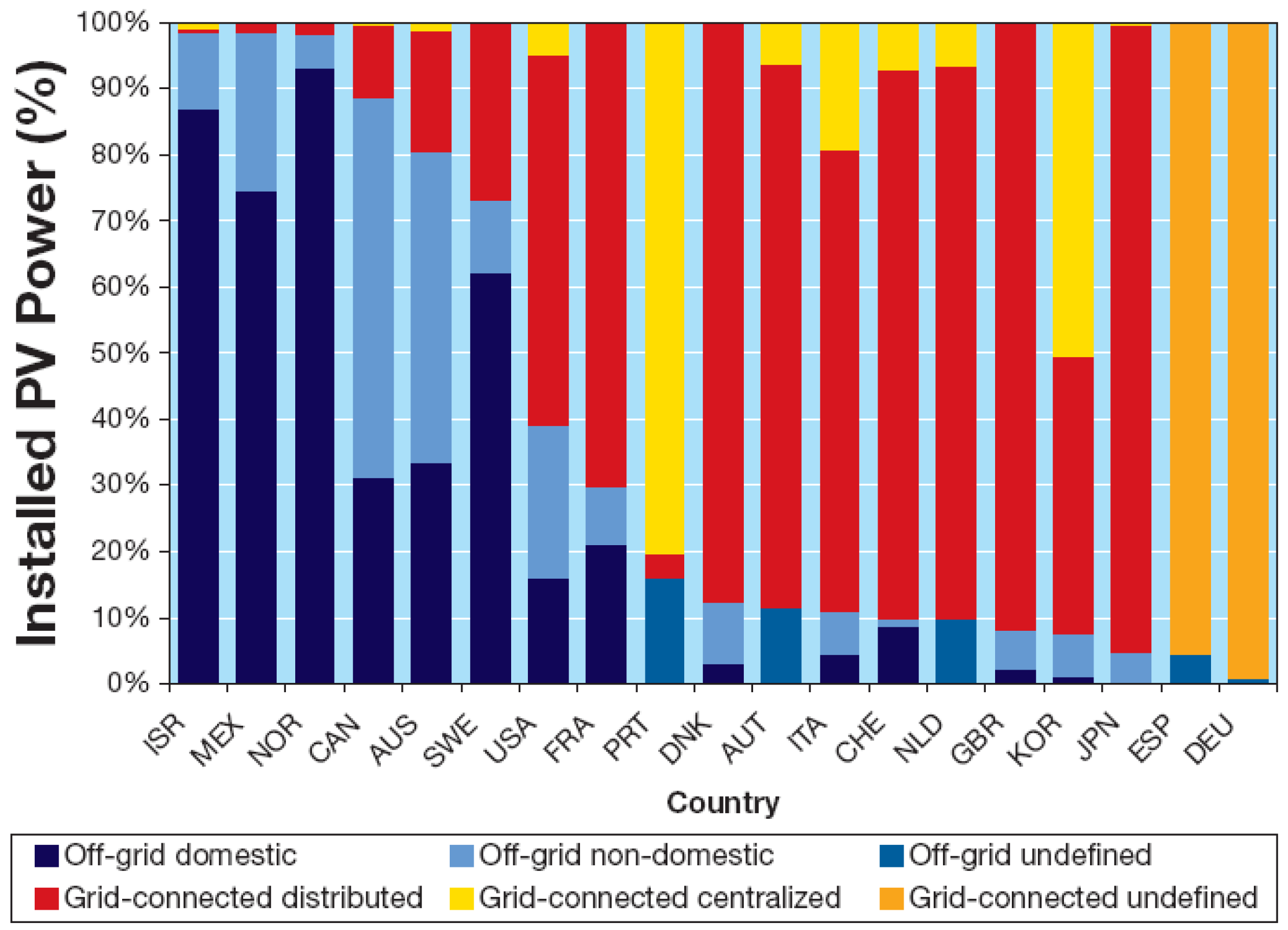
8.3.4. Current scale of deployment

There is a continuum of PV scales ranging from micro applications in pocket calculators, via applications in the 1–5 kW range such as residential rooftops and street lights, mid-range 10–250 kW commercial and industrial applications, to large utility-scale deployment, which is in the order of 500 kW (Mae Hong Son plant, Thailand) or above [258].

8.3.5. Contribution to global electricity supply

In recent years, PV installation has grown by around 40% (Figure 61), which is even stronger than the growth of wind power.

Figure 61. Annual growth in PV installed capacity (after [54]).

However this growth occurs at a comparatively small absolute deployment of about 9 GW (Figure 62). In 2007, 2.26 GW of capacity was installed in IEA-PVPS member countries alone.

Figure 62. Cumulative installed PV power in MW (after [54], [246] and [259]).

This capacity is almost exclusively installed as grid-connected power (Figure 63).

Further, distributed PV applications dominate by far, with significant centralised plant capacity only in the USA, Portugal, Korea and Switzerland (Figure 64).

8.3.6. Cost of electricity output

Electricity from PV systems is considerably more expensive than electricity generated by the power technologies dealt with in the previous four sections. Currently, PV power is economical only in off-grid remote applications.

PV modules represent two thirds of the cost of a PV system in grid-connected systems, with the remainder being for installation and distribution. In off-grid applications however, module cost represent only 30% of cost [251]. In the late 1990s, PV systems cost between 7 and 14 US$/W, but by the time of writing, these costs have come down for installed grid-connected PV power to about 7 US$/W, with the module accounting for about 4.5 US$/W (Table 1 in [55], and Tabs. 6 and 7, and Figure 10 in [54]).

Depending on the insolation profile of the location, PV electricity cost range between 20 and 30 US¢/kWh for stand-alone systems, and between 10 and 18 US¢/kWh for grid-connected systems [55]. PV-based electricity (based on both crystalline and thin film technologies) is not expected to be competitive before 2020 [55]. Technological learning in current niche markets such as remote and off-grid applications, and also internalisation of external costs in fossil electricity are expected to be the main drivers for future cost reductions. Damage cost as found in the EC-US ExternE study suggest carbon prices of around 100$/t, translating into 5–15 US¢/kWh, which is in the order of the current cost gap between fossil electricity and PV [55]. However they may be cheaper ways to mitigate CO₂ from fossil plants such as CCS.

The market for PV-grade silicon is reasonably concentrated with only four major producers worldwide ([251]; Section 2.1 in [54]). Most cells and modules are currently produced in China, Japan and Germany. Ingots, wafers, cells and modules are produced in more countries, for example the UK, Spain, and Norway (see Table 4 in [54], and [260]). As with input materials for other technologies, the price of PV-grade silicon has undergone major increases (2- to 3-fold) between 2003 and 2007 (Section 2.1 in [54]).

8.3.7. Technical challenges

Thin film cells are potentially cheaper to manufacture than crystalline cells, and can be incorporated more flexibly into existing surfaces of all kind (for example vehicles). However they do at present require larger array surfaces because of their comparatively low efficiencies, which in turn translates into higher cost. These high cost present a major barrier for deployment in developing countries, where potential off-grid applications would be most numerous.

Future challenges in bringing kWh cost down lie with improving the performance of PV cells through what Bagnall and Boreland [261] call third-generation PV. Future devices will require significant improvements in efficiency not only at the laboratory scale, but at the commercial scale. Moreover, means to exploit the entire wavelength spectrum of solar light for the excitation of carriers in PV materials are currently explored, such as multi-bandgap multi-junction devices. Another stream of research is directed at creating light-trapping and concentrating cell surfaces. Bagnall and Boreland [261] review the state of research on emerging photovoltaic technologies. Zoellner et al. [241] reports from a survey showing that economic considerations influence acceptance of photovoltaic power, and Fthenakis et al. [248] provide a list of areas where future cost reduction can be expected.

The economic viability of grid-connected PV systems is a complex function of inclination, available capital, load profile, and electricity pricing structure, amongst others, which needs to optimised in order not to over- or undersize PV systems [262]. Many authors propose solar-wind or solar-hydro hybrid power systems in order to overcome the capacity credit limitations of both solar and wind [259]. For such hybridisation to occur at a large scale requires wide regional dispersion, significant improvements of transmission capacity and interconnection (to match spatially distant resources and loads), output forecasting, and peak reserve management.

9. Concentrating solar power

9.1. Summary

The International Energy Agency’s SolarPACES Implementing Agreement (www.solarpaces.org) is one of the collaborative programs under the IEA umbrella. SolarPACES manages research tasks with national organisations such as the US NREL and Sandia laboratories, and Australia’s CSIRO, and coordinates information exchange between member countries on research & development and marketing of concentrating solar power. Mehos [263] provides an overview of SolarPACES Task I, and the status of the technology in 2006.

The bulk of Concentrating Solar Power capacity was constructed in the 1980s and most of it is still operating today. However, no new commercial-scale Concentrating Solar plant has been commissioned until recently, so the technology has been described as “matured, stalled, and recently invigorated” [56]. Concentrating Solar Power integrates well with existing fossil power infrastructure, exhibits good load matching in sunny regions, has a high capacity credit with hourly storage, and is flexible in deployment because of its modularity. Its major barrier is currently uncompetitive cost, which are projected to achieve grid parity only around 2020 and only with strong government incentives.

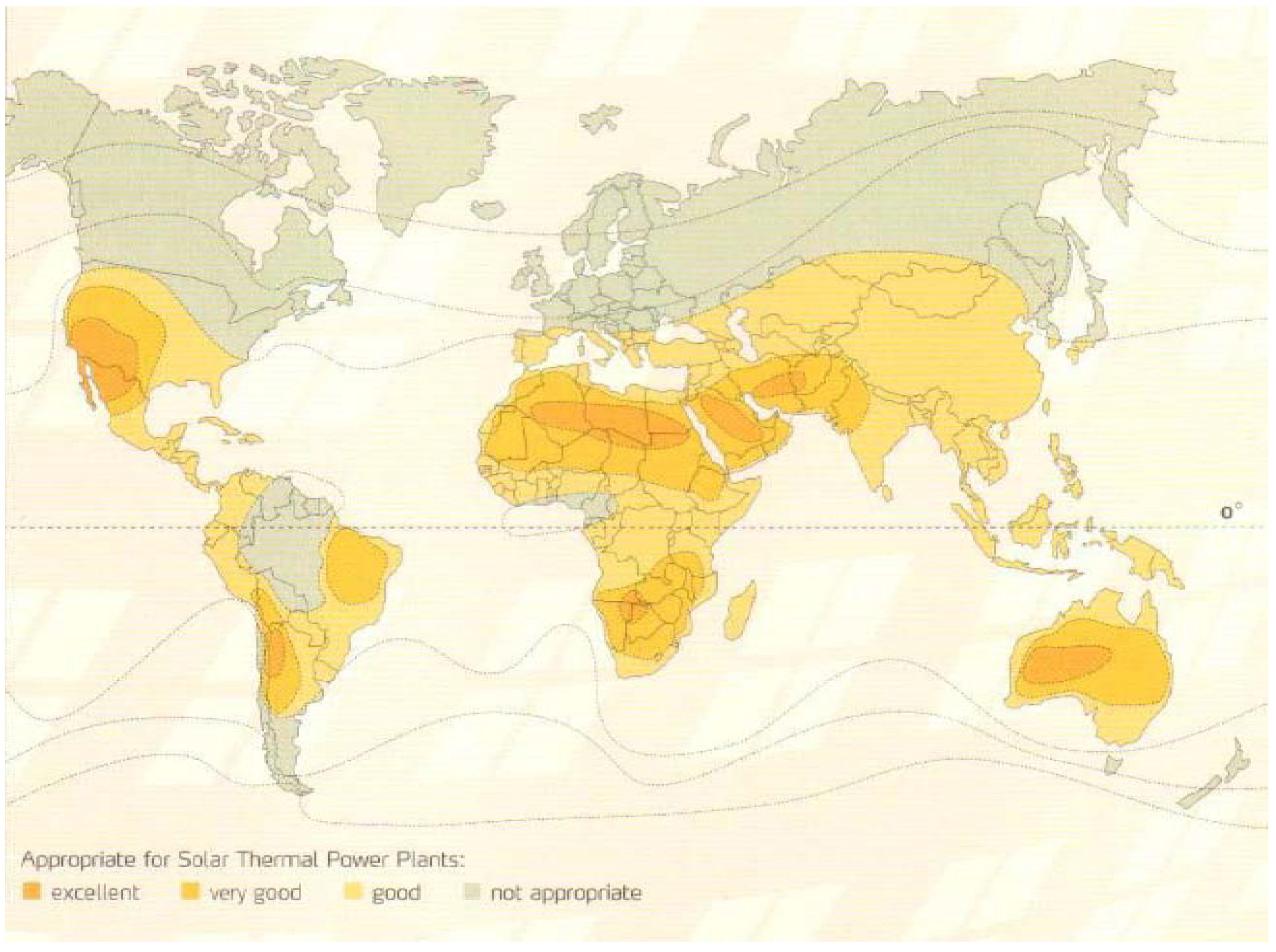
9.2. Global potential of resource

The technical potential of Concentrating Solar Power varies between studies, but agreement exists that it is much higher than the world’s current electricity consumption [264]. The economic potential lies in the world’s sunbelts ([2], Figure 65).

Several studies commissioned by high-level organisations such as the US DoE and the World Bank ([266], US DoE and [56]) put the 2020 economic potential of concentrating solar power at around 20 GW, the DLR estimates 10 GW, and the IEA and DLR estimate 40 GW [194,267]. The CSP Global Market Initiative deployment target is 5 GW by 2015 [268]. Fthenakis et al. [248] project US deployment at 120 GW in 2030, 1,500 GW in 2050, and 5,000 GW in 2100. The ACT and BLUE scenarios of the IEA [2] project 2050 potentials between 3% and 5.5%. However, past projections such as the one by Trieb [269] forecasting 7 GW in 2007 proved to be incorrect.

A recent key proposal for the utilisation of concentrating solar power – led by the German Aerospace Centre (Deutsches Zentrum für Luft- und Raumfahrt; [270]) – is to link Central Europe’s population and load centres to 20 GW of solar power sources in the Mediterranean and North African “sunbelt” via low-loss and low-cost high-voltage DC transmission lines, by 2020 [192,268,271]. Ummel and Wheeler [272] undertake a GIS analysis of the potential of this proposal, taking into account unsuitable areas (protected areas, shifting sand dunes, corrosive salt plains, settled areas, inland water bodies, sloped terrain), proximity to transport infrastructure and existing transmission corridors. Two routes for cross-Mediterranean transmission were selected according to sea bed depths of less than 2 km: the Strait of Gibraltar, and Tunisia, Sardinia, Corsica to the Italian mainland. Ummel and Wheeler [272] conclude that even with modest carbon prices, Concentrating Solar Power in North Africa would be 1.5–2 times more expensive than state-of-the-art coal and gas technologies. For distances between 2,000 and 3,000 km, high-voltage DC transmission would add about 3 US¢/kWh [194,264]. A drawback is that many countries located in the sunbelt do not have the financial resources necessary to afford Concentrating Solar Power, so that only those in proximity to potential sponsors would be candidates for deployment [264]. Another challenge is creating and nurturing a political climate that encourages international cooperation and that guarantees energy security [195]. Mitigation potentials are very uncertain, but an indicative estimate is given by Brakmann et al. [266] to be 362 Mt CO₂ up to 2025. Projecting Concentrating Solar Power to 40 GW in 2030, 350 GW in 2050, and 2,800 GW in 2,100 would yield a mitigation potential of about 150 Gt CO₂.

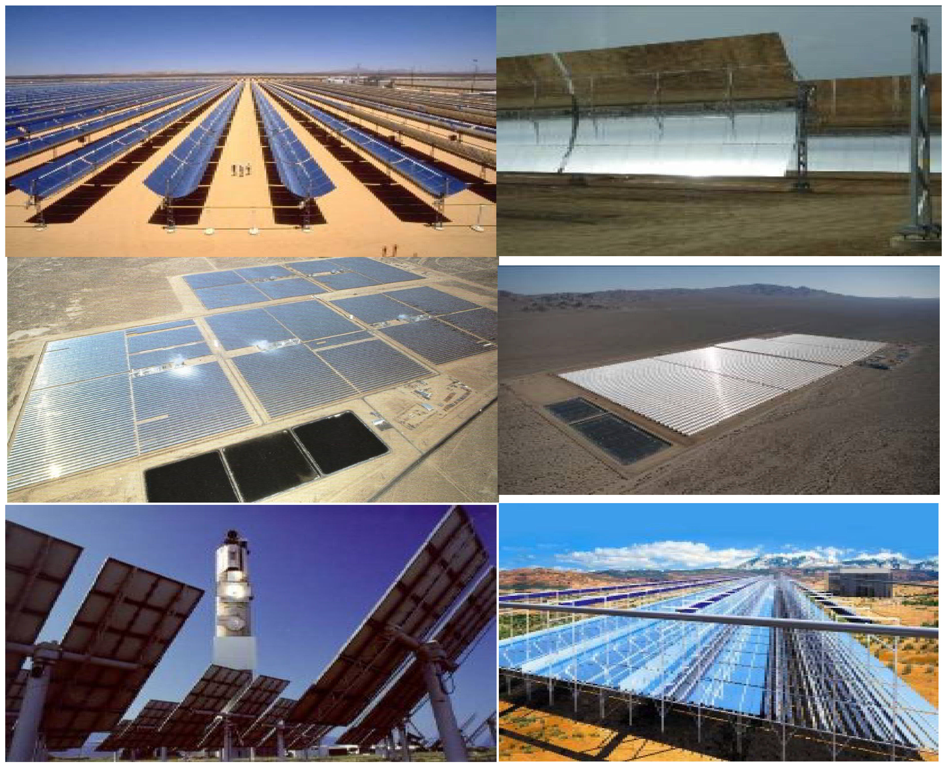
9.3. Solar-thermal troughs, dishes, towers, and Linear Fresnel systems

9.3.1. Technical principle

Solar-thermal energy is perhaps best known for the widely used low-temperature solar collectors that provide residential hot water and space heat. This Section deals with Concentrating Solar Power systems, also referred to as solar-thermal power. The basic idea is to concentrate sunlight onto receivers, where it heats a heat transfer fluid (for example molten salt, oil) to a temperature sufficient to generate steam to drive a turbine. The higher the transfer fluid temperature, the higher the maximum conversion efficiency (the “Carnot limit”; [273]). Plant designs using direct steam generation avoid the need for a heat transfer fluid and associated heat exchange cost and losses ([274]; p. 22 ff. in [275]).

There are at present four basic designs ([275]; Figure 66). A dual-axis tracking parabolic dish focuses light onto a receiver that sits in its focal point, and that is coupled to a Stirling or steam engine [276]. Because of the point-focusing, dish systems achieve high temperatures and efficient conversion. Single-axis tilting parabolic troughs focus light on receiver (vacuum) tubes running along the focal line of the trough mirrors [277]. The trough-and-tube design avoids the need for dual-axis tracking. Linear Fresnel technology does away with moving parts and fluid couplings typical in dish- and trough-mounted receivers, by using slightly curved or flat mirrors to focus light onto stationary linear receivers. In Compact Linear Fresnel designs, mirrors can be aimed at different receivers throughout the day and thus optimise optical efficiency over time, as well as achieve a dense area packing [278,279]). Central receiver plants (also called “power towers”) are surrounded by a field of dual-axis tracking mirrors (“heliostats”) that are focused onto a tower-mounted single central receiver. Similar to parabolic dishes, such plants are able to generate high-temperature heat that can be converted to power more efficiently. Stretched-membrane heliostats are able to focus their own sun image onto the receiver rather than just a plane beam [273]. Multi-tower solar arrays have been proposed by Schramek and Mills [280,281].

Figure 66. Parabolic troughs (top row), parabolic trough plants (middle row) SEGS (left) and Nevada Solar One (right), central receiver Planta Solar (bottow left) and Linear Fresnel plant (bottom right), both in Spain. Figure reproduced from [282] with permission.

Concentrating solar power is a thermal technology and thus, unlike photovoltaic power, has the ability of being integrated with other (nuclear and fossil) thermal power plants by pre-heating water to be turned into turbine steam, or by adding steam. For example, in Integrated Solar Combined Cycle (ISCC) plants, solar concentrators are combined with gas-fired combined-cycle plants. Depending on the ratio of integration, either the solar plant operates as a fuel-saver (typically 15% of total hybrid capacity, or the fossil plants acts as back-up (typically 25% of total hybrid capacity; [194]). In combination with the ability of concentrating solar plants for short-term storage and thus high capacity credit, these plants are suited for grid integration without major changes to the grid structure [194]. Given that concentrating solar plants would mainly be installed in sunny arid regions, the waste heat from the plants can also be used for seawater desalination [264,283,284].

Concentrating solar power can be transmitted at low cost and low losses over distances in excess of 1,000 km, as is done routinely (60 GW worldwide; [264]) in China, India, the USA, and between Tasmania and the Australian mainland [194].

9.3.2. Capacity and load characteristics

The average capacity factor of the SEGS parabolic trough plant is 21%, whilst that of the PS10 central receiver is 24%. Short-term (hourly) storage of solar heat provided by the heat transfer fluid itself and additional molten-salt storage tanks avoids fast ramping of the conventional plant. Optional longer-term storage means that the plant can also produce during extended low-radiation periods, thus significantly increasing its average capacity factor and its capacity credit. In contrast to the US parabolic trough plants, the Spanish Andasol trough plants have a liquid salt storage system that allows them to operate day and night at an average capacity factor of 41%, and make more efficient use of a smaller generation unit [285].

Storage and fossil hybridisation capability means that concentrating solar plants achieve high capacity credits, thus making them candidates for highly reliable power supply. Based on Californian SEGS experience, the solar component was able to supply power in around 80% of peak load situations. However, in sunny climates with high midday loads (such as California), Concentrating Solar Power has favourable capacity credits comparable to those of photovoltaic power, even without storage. DLR [270] gives a wide range of capacity credit ranging from 0% without storage to 90% with storage and hybridisation/back-up.

9.3.3. Life-cycle characteristics

Lenzen [36] carries out an input-output-based life-cycle assessment of parabolic trough, dish, and central receiver technologies, and arrives at values around 0.3 kWh_th/kWh_el, and between 50 and 90 g CO₂-e/kWh. As expected, the greenhouse gas intensity decreases with increasing storage and capacity factor (Figure 67). Lenzen and Treloar [286] show, for the example of concentrating solar technologies, that it is essential to achieve complete upstream coverage in a life-cycle assessment.

Figure 67. Greenhouse gas and energy intensities of Concentrating Solar Power as a function of average capacity factor (CR = Central Receiver, PT = Parabolic Trough). © 1999 Elsevier, reproduced with permission from [36].

Land requirements of concentrating solar plants are below those for biomass and hydroelectric power [194]. Since mainly sunny, arid regions are targeted for deployment, land competition can be expected to be low [272].

The effect of Concentrating Solar deployment on the wider economy and employment has been enumerated in an input-output analysis of Spain by Caldés et al. [287]. While this methodology is appropriate for answering questions of economic and environmental flow-on effects [288], there are not many comparable studies that cover other technologies. Many arguments of employment effects of power technology have been made based on process analysis, which is affected by systematic truncation errors. Such truncation errors are demonstrated in Table 3 in [36] for the example of embodied energy and greenhouse gases for a central receiver plant. Notwithstanding the above, the positive effects of Concentrating Solar Power projects on employment, economic development and water security in developing countries has been noted [270].

9.3.4. Current scale of deployment

The largest operational concentrating solar power station (and the largest solar power plant in the world) is the 354 MW SEGS parabolic-trough plant in the US’ Mojave desert, incorporating nine units built between 1984 and 1989 [273]. There are two more parabolic-trough plants: Nevada Solar One, 75 MW, in Nevada, USA, and Andasol, 50 MW, in Andalucía, Spain. At present there is only one operational central receiver (PS10, 11 MW), which is located near Seville, Spain; the 10 MW Solar One plant in the US has been decommissioned. The US company Ausra has built a 5 MW LFR demonstration plant, and also Australia’s Liddell power station features a concentrating solar booster plant (360 kW) based on the LFR principle. A small CLFR demonstration plant has been operated at the Stanwell power plant in Rockhampton, Australia [289]. The largest single parabolic dish prototype is the Australian National University’s SG3 with a rated capacity of 45 kW. The largest distributed dish array was built in California in 1983/1984 with a nominal output of 4.9 MW [273]. DLR [270] provides a range of deployment sizes between 10 kW and 200 MW. The modular structure of concentrating solar plants means that they can produce power at any size [194].

9.3.5. Contribution to global electricity supply

The current deployment of concentrating solar power is about 450 MW, with an additional 500 MW (exclusively plants below 75 MW rated capacity) under construction, and some 7 GW announced [290]. Given capacity factors of around 25%, the annual electricity output is about 985 GWh.

9.3.6. Cost of electricity output

The levelised cost of concentrating solar power are reported to be around 15–25 US¢/kWh, which is currently uncompetitive [56,267], except in circumstances where both insolation and conventional electricity costs are high, for example parabolic dish systems on sunny islands [291], and in sunny remote areas [292]. Most of these costs are due to high upfront investments, and only about 4 US¢/kWh are due to continuous operation. In case of large distances between plants and loads, high-voltage DC transmission would add about 3 US¢/kWh [194]. Quaschning [293] shows that, because of their additional cost of tracking, Concentrating Solar Power plants are more competitive in locations with high solar irradiation. The Californian experience shows that plant lifetimes are at least 25 years. As the plant lifetime extends, levelised electricity costs are decreasing further towards their lower limit posed by the long-term operating cost. IEA, US DoE and World Bank estimates put 2020 levelised cost of concentrating solar power at below 6 US¢/kWh (Figure 68; [194]).

Figure 68. (a) Historical and anticipated decrease in generation cost with increasing production (Reproduced from [268] with permission). (b) Historical and anticipated decrease in generation cost over time (after [294]).

However, this will require a re-activation of R&D and financial support for market introduction, because technological learning has essentially stalled after the completion of the last SEGS plant at the end of the 1980s (Figure 69). Another challenge will be to decrease interest rates on capital borrowed for building new plants, because at present, investors view Concentrating Solar Power as a high-risk technology ([275], p. 17).

9.3.7. Technical challenges

The main challenge for solar concentrating power is to reduce cost, for example by improving performance and long-term reliability at reduced material input ([267], p. 16 ff.; [275], p. 17 ff.). This includes the development of direct steam generation technology, the increase of collector length and associated reduction of tracking devices, reduction of stresses on mirrors, development of air receivers for power towers, and testing of solar syngas, metal and hydrogen production. No major scientific breakthroughs are required for cost reductions [56]. Anticipated cost decreases are expected to come half from such technological innovation, and half from upscaling ([267,294] Fig. 1-5). Another aspect is achieving higher outlet temperatures which would result in higher thermal conversion efficiencies [194]. Various designs have been proposed that involve heat storage systems using molten salts, steam, graphite, or phase-change materials in order to increase the average capacity factor of concentrating solar plants. Research at the Australian National University is directed at the development of thermochemical energy storage using ammonia [295]. Other designs include the usage of concentrating solar heat for the reforming of fuels for multiple purposes, electricity generation being one of them [296,297,298,299].

10. Geothermal power

10.1. Summary

The status of geothermal electricity generation is very well documented, notably in the on-line information of the International Geothermal Association (www.geothermal-energy.org), and in the work of DiPippo [300,301]. The geothermal resource is characterised by one of the largest technical potentials amongst all renewable energy sources, as well as true base load capability, simple and mature technology, low environmental impact, and near-competitive cost between 6 and 8 US¢/kWh. It is therefore surprising that growth rates of geothermal deployment have only been moderate—an average of 4% over the past decade. The only barrier appears to be the upfront uncertainties about the generating capacity of geothermal fields, which only reduce whilst the field is commercially exploited, thus often requiring a step-wise and drawn out development approach in order to avoid mismatches between field and power plant capacities, as well as to minimise the risk to investors.

10.2. Global potential of resource

It is widely accepted that the technical potential of geothermal energy exceeds current global energy consumption many times [205,302,303] (the US study in [302] assumes depths of up to 10 km). This is also true in many cases at the national level, for example in the USA, where technical and economic potentials have been estimated to be 2000 and 10 times higher than current demand, respectively [302].

Fthenakis et al. [248] project US geothermal deployment at 55 GW in 2030, 100 GW in 2050, and 200 GW in 2100. A report by MIT [302] more closely investigated the 2050 target, and concluded that starting from around 2020–2025, US geothermal capacity could be ramped up to reach 100 GW of base load in 2050. The report also concluded that the lack of attention paid to the geothermal resource led to the false perception that the technology was associated with technical barriers, and with limited to relatively scarce hydrothermal resources. To this end, the report states (pp. 1–4): ”Initial concerns regarding five key issues – flow short circuiting, a need for high injection pressures, water losses, geochemical impacts, and induced seismicity – appear to be either fully resolved or manageable with proper monitoring and operational changes”. The 2050 global potential is estimated in the ACT and BLUE scenarios of the IEA [2] as about 200 GW.

At growth rates leading to global deployment of 350 GW of geothermal power by 2100, the mitigation potential would be in the order of 25–50 Gt CO₂. More rapid deployment scenarios leading to 3,500 GW deployment by 2100 could, depending on the expansion path, mitigate 250–500 Gt CO₂. The likelihood of either scenario is uncertain.

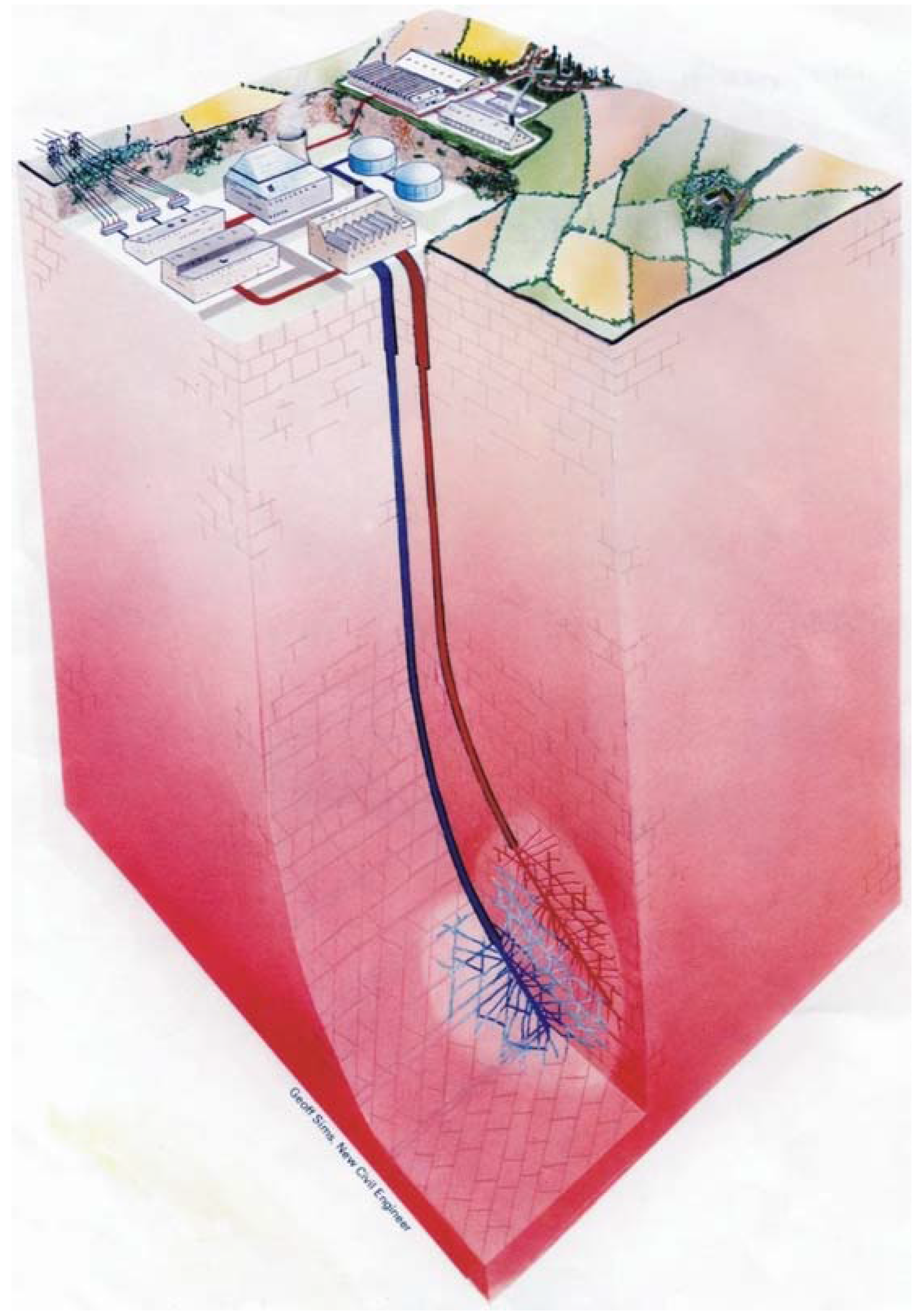
10.3. Geothermal power plants

10.3.1. Technical principle

Geothermal power derives electricity from energy flow in the Earth’s crust (derived mainly from convection and conduction of heat from mantle and core, and from the decay of radioactive crustal elements such as uranium and thorium), and thus does not require additional energy storage to generate base load power. Geothermal power development depends critically on the successful exploration, drilling and management of geothermal resources [304]. The quality, or grade of a geothermal resource is determined by its geothermal gradient, its permeability and porosity, and its fluid saturation [302]. The resource temperature in turn determines the conversion technology.

Binary-cycle geothermal power plants utilise water of relatively low temperature (<200 °C), which is pumped from a geothermal reservoir (a geothermal reservoir contains hot water or steam that is trapped in permeable and porous rocks under a layer of impermeable rock [303]) through a well, and made to exchange heat with a working (binary) fluid of low boiling point which in turn drives a turbine The geothermal fluid (geofluid) hence operates in a closed cycle. Binary-cycle plants are the most numerous type of geothermal power plant, but since they are generally small, they only produce about 4% of geothermal power [305].

In a “single-flash” plant type, the geofluid has undergone one flash evaporation (flash evaporation mean that a pressurised liquid is converted into a gas by suddenly lowering the pressure of the liquid below its saturation pressure at the respective temperature), which can occur either in the geothermal reservoir as the fluid flows through formations of decreasing pressure, in the well as the gravity pressure drops on the way up, or during throttling at the inlet valve or plate of a separator. There it is separated into distinct steam and liquid phases, with the steam used to drive the turbine [306]. A “double-flash” plant can produce 15%–25% more output under the same conditions compared to a single-flash plant, by producing additional low-pressure steam from the liquid, using a dedicated flasher installed at the surface. The low-pressure steam is admitted into the turbine at a stage downstream from the high-pressure inlet [307].

“Dry-steam” resources of higher temperature are preferred, because they avoid the need to separate the condensed phase out of the steam before injection into the turbine. They tend to be less expensive that flash-steam plants, because the geofluid contains only steam and no brine. However, dry steam resources are also less abundant, and at present exploited on a large scale only in the USA and in Italy [308].

The Hot Dry Rock (HDR) technology uses two wells. Water is injected into one well, gets heated while travelling through the porous rock, and is forced out of the other well before being fed into a steam turbine or into a heat exchanger (Figure 70). The term Enhanced Geothermal Systems (EGS) describes an extension of the HDR technology in that it uses engineered subsurface fracture system for circulating the water [303]. Most EGS are imperfect resources in that they lack at least one of desired characteristics—large geothermal gradient, large permeability and porosity, and high fluid saturation [302]. A further challenge is creating sufficient connectivity between injection and production wells in order to achieve high production rates whilst avoiding rapid cooling. However, EGS systems with naturally low permeability also represent the largest crustal heat resource.

In 2005, most of operating geothermal power plants (42%) were of the binary type, followed by single-flash plants (26%), double-flash plants (14%), and dry steam plants (12%; [309]). Geothermal plants have a higher heat rejection ratio (typically 90%) compared to conventional thermal power plants; they are ideally suited for combined heat and power generation. Geothermal wells deplete during their operational lifetime, but recover if left for several decades.

Noncondensable gases such as CO₂ (typically 95%) and H₂S (1%–2%) that are contained in the geothermal fluid are removed from the condenser, in order not to raise the backpressure of the turbine. This comes at the cost of some steam, but in the long term yields a higher net power than a setting in which the noncondensable gases were left to accumulate [311]. In plants that use air-cooled condensers, the generating efficiency shows a seasonal dependence on the ambient air temperature, with decreases during summer peaks. In these cases, power output can be improved by incorporating water-cooling into the condenser system [312].

10.3.2. Capacity and load characteristics

Geothermal power is regarded as the only renewable energy source that is entirely independent of seasonal or climatic changes, thus allowing it to achieve high capacity factors in excess of 90% [313,314]. In 2005, 9,084 GW of geothermal power generated 56,951 GWh of electricity [315], which is equivalent to an average capacity factor of 71%.

10.3.3. Life-cycle characteristics

Geothermal and volcanic systems are natural emitters of CO₂. These emissions can increase during the opening of a geothermal field for power production, however in other cases natural emissions have decreased as a result of development. Emissions attributable to the power plants are usually obtained by subtracting pre-development emission levels [57]. There exists a debate on whether emissions attributable to power development form a significant portion of naturally occurring emissions. Ármannsson et al. [57] update previous research and conclude that circumstances vary with the location of the fields. For example, Italy does not include any CO₂ emissions from its Larderello field in its national inventory communication to the IPCC, but this would not be possible for fields in Iceland and New Zealand. A survey of CO₂ emissions from geothermal power plants yields a large range of 4–740 g/kWh, with a weighted average of about 120 g/kWh [57]. DiPippo [311] gives a lower range between 50 and 80 g/kWh, and Kagel et al. [316] state 44 g/kWh. None of these emissions include upstream stages of the power plants’ life cycles.

In contrast to CO₂, emissions of H₂S are currently already strictly regulated. H₂S can either be chemically scrubbed from the geofluid, or alternatively the noncondensable gases can be compressed and reinjected into the geothermal reservoir [311].

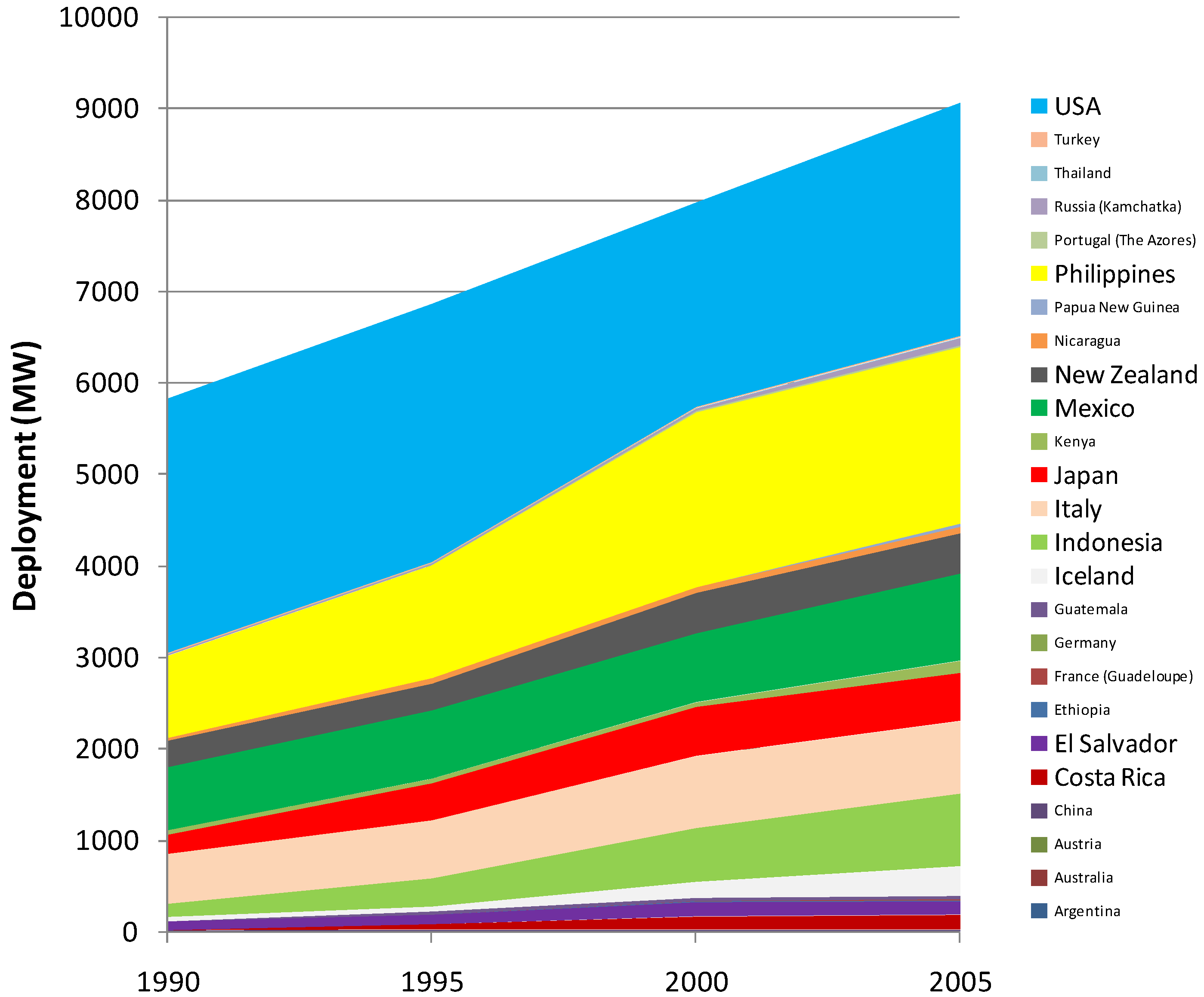
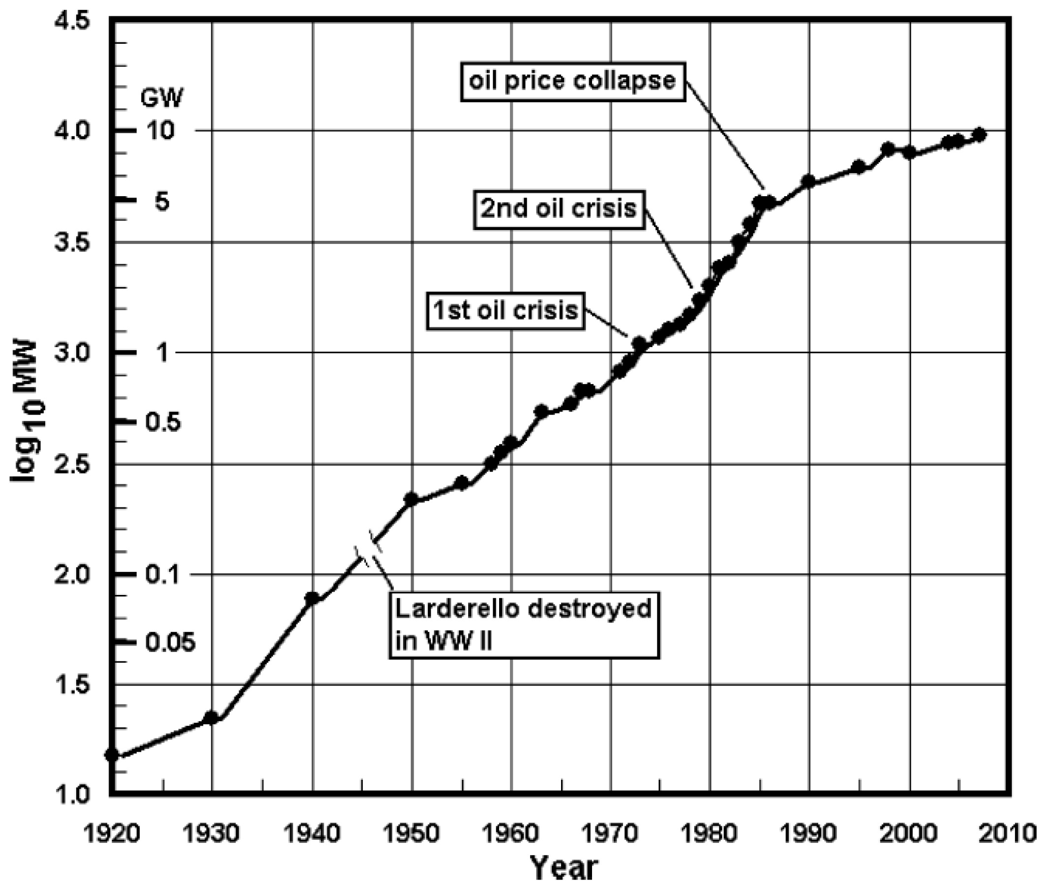
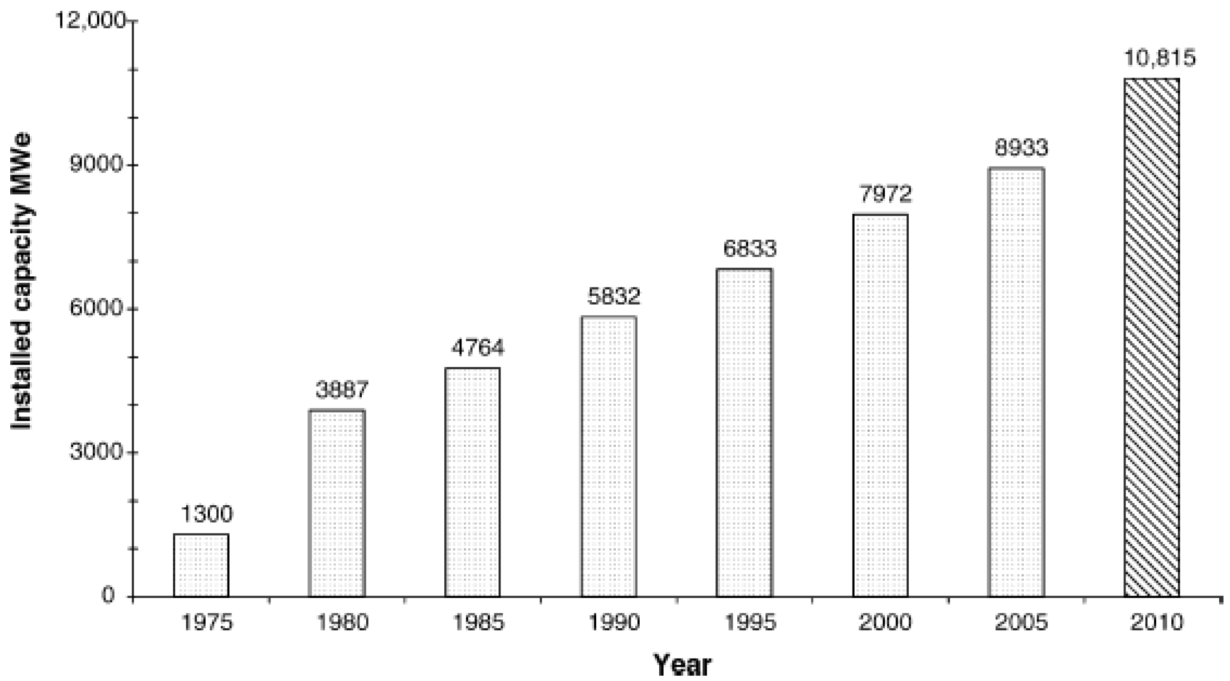
10.3.4. Current scale of deployment

The largest assembly of geothermal power plants are “The Geysers” in the USA, combining some 22 single plants into a 750-MW power plant park [317]. Excluding smaller binary plant units, the average size of dry steam, single- and double-flash plants is about 30 MW [309]. Including all plants, the average size is about 19 MW (Table A.5 in [301]). Geothermal field output can be measured in units of MW per km drilled. In measurements of geothermal fields in the Philippines and New Zealand, this parameter varied around 3.5 MW/km (Figure 4 in [314]).

10.3.5. Contribution to global electricity supply

Geothermal power is installed currently in more than 20 countries around the world. On a regional basis, geothermal power contributes significant amounts (15%–20%) to total electricity generation only in two countries: the Philippines and Iceland. Total installed capacity is close to 10 GW (Figure 71).

Figure 71. Deployment of geothermal power (derived from data in [318]).

DiPippo [301] collates historical data and demonstrates the effect of the oil price collapse in the mid 1980s on geothermal power deployment (Figure 72).

Since the oil price collapse, deployment has only grown linearly at an average of about 200 MW of additional capacity per year, since 1975 (Figure 73). Current growth rates have been around 3%, down from about 15% after 1979. In 2005, 56,951 GWh of electricity were generated from geothermal sources [315].

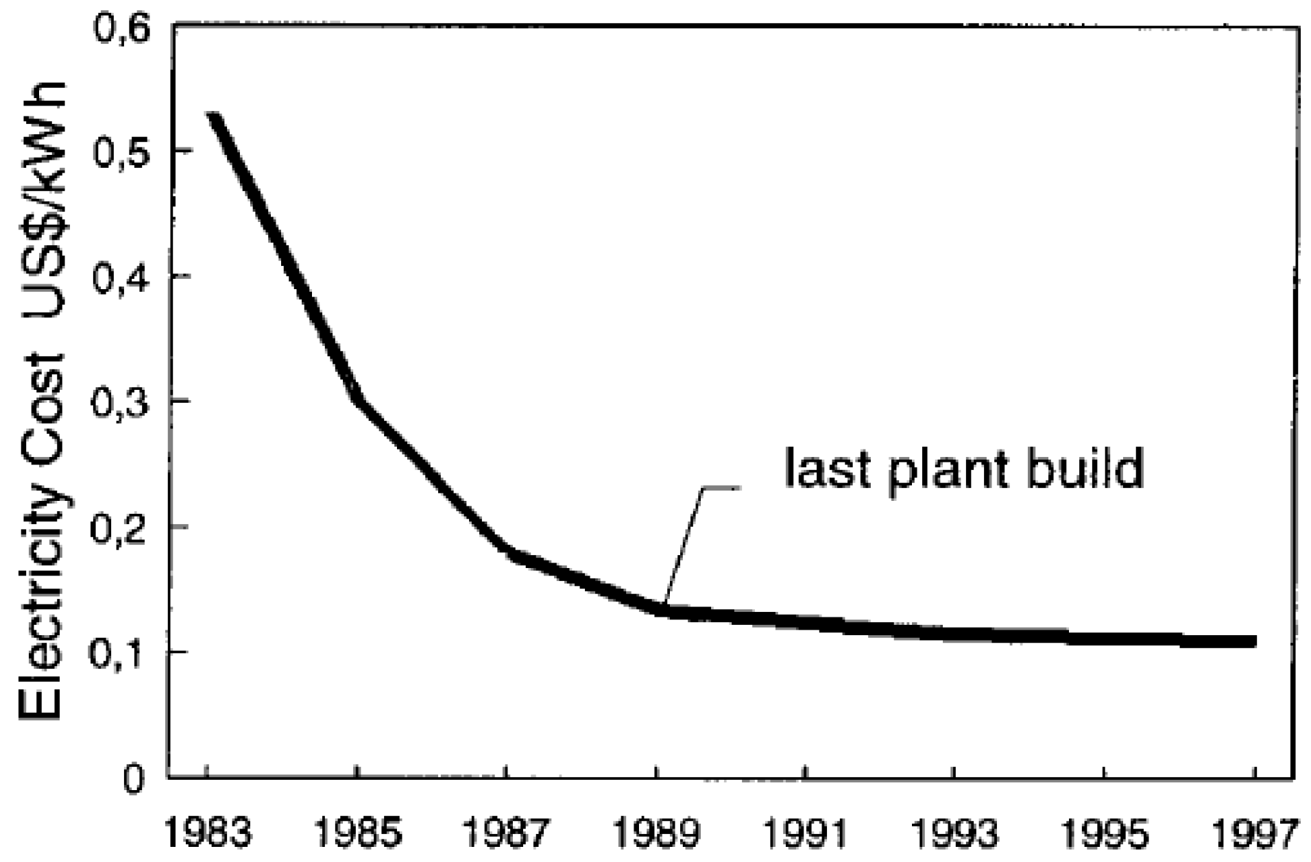
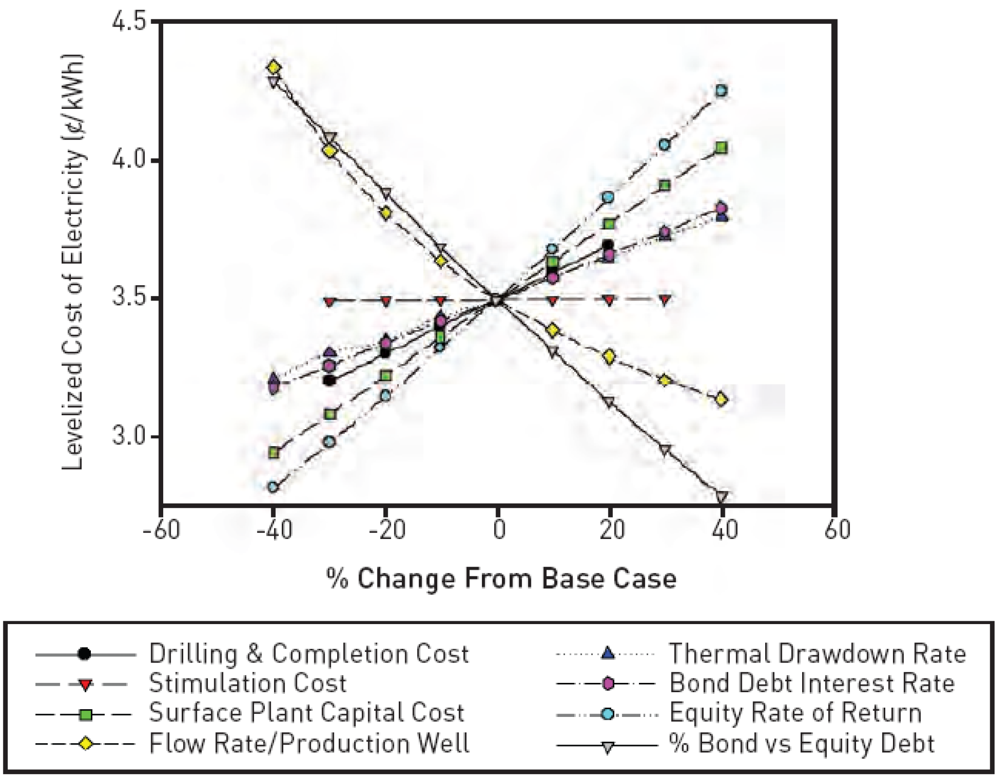
10.3.6. Cost of electricity output

Geothermal generating cost, and especially upfront capital costs are quite resource- and site-specific [319]. Investment cost for geothermal power plants include surface infrastructure and equipment and subsurface infrastructure. The cost of the latter are more variable (10%–50% of total cost) because different requirements in low- and high-temperature geothermal fields, and also more uncertain because reliable estimates of the generation capacity of a geothermal reservoir can only be obtained once the reservoir has been tested under production. Subsurface cost can be assumed as increasing linearly with the number of wells [314].

Matching of the generating capacity of the geothermal field with the sizing of the power-generating equipment is important in order to optimise investment strategies. This suggests a step-wise development of geothermal resources, with system expansion being undertaken in 20–30 MW units, as practised in Iceland. However, such a strategy also implies delays of up to 6 years between the drilling investment, and the financial returns from power production, so that conflicting goals must be managed [314].

There are some trade-offs between cost of different plant designs. For example, a discharge-to-atmosphere design would avoid the installation of a re-injection system, but would need additional costly wells. Hot geothermal fluids could be transported by pipeline, however in order to decrease cost, the distance between the location of the resource and its utilisation should be kept as short as possible. As with conventional systems, combining heat and power applications has positive effects on cost [310].

Current electricity cost range between 2 and 10 US¢/kWh [310], US plants in 2005 were operating for about 5.5 to 7.5 US¢/kWh [58], and for around 8 US¢/kWh in 2007 [303].

The main factors driving up levelised costs are interest rates on debt, and equity rates of return, as well as cost of upfront capital. The main factor driving down levelised cost is the flow rate in the production well (Figure 74).

10.3.7. Technical challenges

Immediate R&D needs exist in the areas of drilling and power conversion technologies, including casing methods, downhole tools and electronics, and high-temperature turbines. Reservoir technology is also a crucial R&D area because significant cost reductions can be achieved through careful identification and management of subsurface systems, including the targeting of specific EGS zones with differentiated production rates, remedy of subsurface short-circuits.

Geothermal wells and power plant operations can adversely affect the geological stability of the local region, for example through land subsidence and increased seismicity [311,316]. Care must also be taken to separate geothermal fluid from surface and groundwater bodies, in order to avoid environmental impacts due to either thermal pollution and its effect on aquatic wildlife, and chemical pollution [310,316]. The well casings therefore must be designed and installed so that ruptures under thermal stress and corrosion by the geofluid can be minimised [311].

11. Biomass

This Section deals with biomass for electricity generation. However, frequent reference is made to biofuel production, with the main application being for transport fuels. This is done because first, biomass for power generation shares many of the features and criticisms with biofuels, particularly with regard to the production of feedstock. Second, since biomass for power purposes is secondary to fuel production, more data (for example on life-cycle performance) can be found for studies dedicated to biofuel applications. Post-harvest, the biomass power path leads to firing, co-firing or gasification, whilst the biofuel path leads to refining into a liquid fuel.

11.1. Summary

Biomass occupies only a small role in global electricity supply. Currently, biomass co-firing of agricultural and forest residues and municipal waste in coal-fired power plants is the most effective use [320]. Dedicated biomass power plants use mostly residues and waste, and are small because of limited feedstock availability and transportation cost. Integrated gasification of biomass is under development, but currently only implemented for combusting black liquor in combined-cycle plants in pulp and paper industries. Future biomass processing is likely to occur in so-called biorefinieries where a range of feedstocks is turned into a variety of energy carriers, such as liquid biofuels, biopolymers, biogas, hydrogen or electricity [321]. A key challenge here is the development of both cost-effective and efficient gasifier/turbine technology for biomass feedstocks [59]. In long-term low-carbon scenarios, biomass has a role for replacing gas as reserve capacity for variable renewable such as wind, solar-thermal and PV [248]. Feedstock availability is a barrier for large-scale future deployment, unless attractive and internationally tradable dense feedstocks can be developed. At least in the countries that depend on imported oil for transportation purposes, dedicated energy crops may have more value as biofuel feedstock rather than fuel for power generation [302,322,323].

Expansion of biomass production for energy purposes has been widely associated with the potential for diverting farmland, water and/or crops to the detriment of global food supply, with potentially adverse impacts on biodiversity because of unsustainable production methods including land clearing, and with food price increases hitting the world’s poorest people [324,325]. Adverse impacts exist even for agricultural residues, because they are diverted away from animal feed and manure [326], which has the potential to disrupt nutrient cycling, deplete soil fertility [327]. The debate is still controversial; effects may vary between crops and locations, and farmers in developing countries may also benefit from increased employment opportunities and earnings from a valued resource [328,329]. Biofuels also have the potential for enhanced energy security, environmental performance, foreign exchange savings, and socioeconomic benefits for rural population segments [330]. In any case, the debate has stimulated increased research into the potential of non-food (2^nd–generation) biomass [328]. Unless such biomass is restricted to various kinds of residues and wastes that are not used even as livestock feed [326], or occurs on land not usable for competing purposes [331], dedicated energy crops would still uphold competition over land. Finally, incineration of waste often faces public acceptance issues.

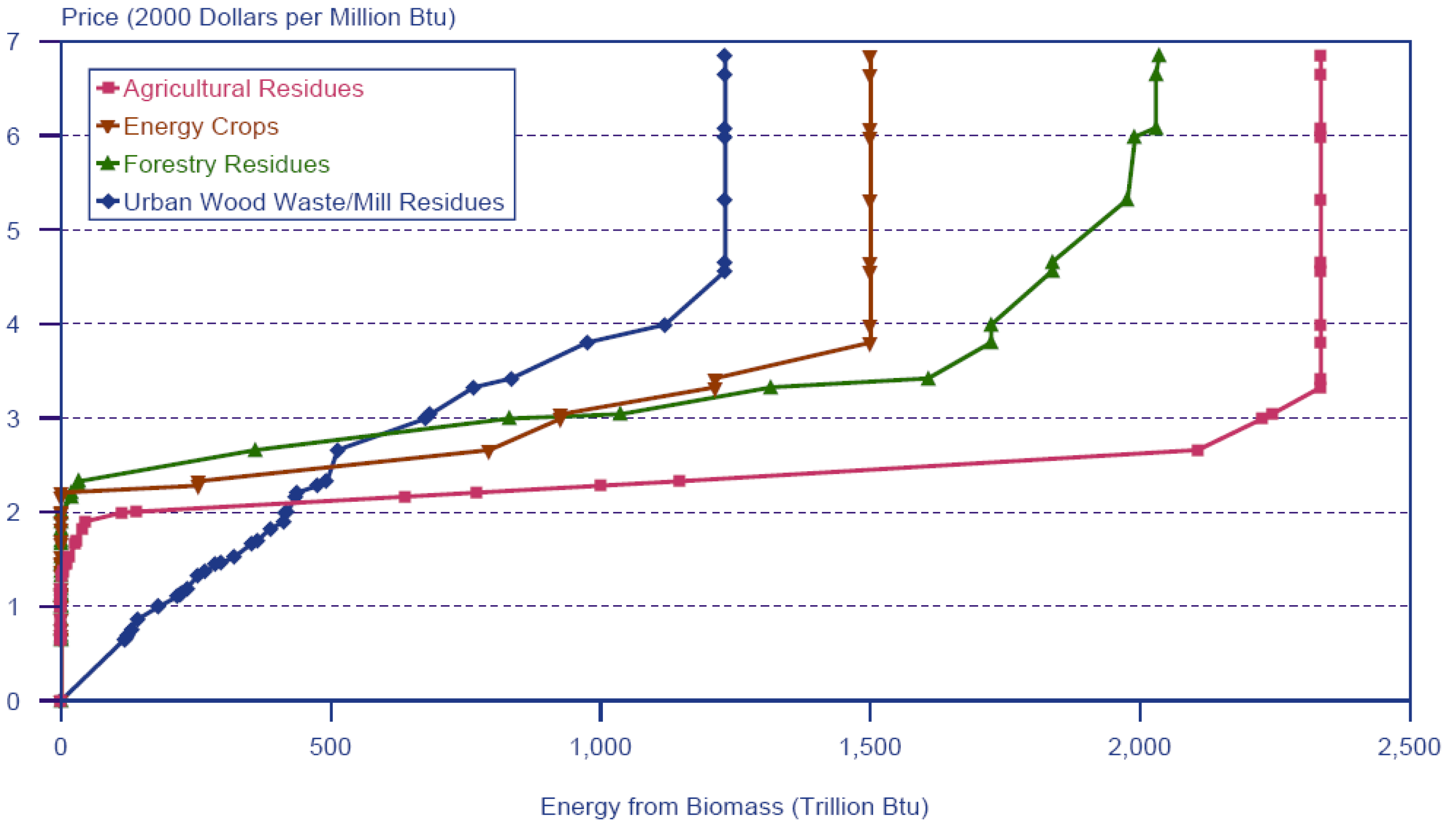
11.2. Global potential of resource

The future potential of the biomass resource is dependent on the ability to cost-effectively and efficiently utilise 2^nd-generation biofuels produced from residues and waste not utilised elsewhere, or from energy crops grown on abandoned agricultural land. This is not expected until at least 2020, and until then, the competition of biofuel production with food and biodiversity objectives and hence limited availability and tradability of biomass feedstock for power generation purposes will keep growth rates for biofuel utilisation at moderate levels. Sims et al. [328] cites a US DoE study that forecasts a moderate level of 13 GW of biomass power by 2010. Perlack et al. [332] cite a US BTAC study projecting a 2% annual linear growth of biomass for power purposes through 2030. Haq [333] lists a projection for the USA of 11 GW biomass-fuelled power by 2020, generating around 70 TWh/y of electricity, most of which (75%–80%) occurs in industrial co-generation, with the remainder in general power plants. This trend corresponds to a 2.5% annual growth. These estimates are consistent with results from the World Biomass Report, summarised by Knight and Westwood [334], showing annual capacity increases of between 800 and 1600 MW until 2013, representing between 2% and 2.5% of global capacity. On the global scale, IEA [59] estimates that biomass power may represent between 3 and 5% of global power generation by 2050.

If biomass utilisation is to expand to significant scales without exerting pressure on competing land use purposes, the portion of residues and waste not utilised for other purposes has to be as large as possible. Haq [333] gives supply curves for four types of biomass available in the US in 2020, showing that agricultural and forestry residues have the largest potential contributions to biomass supply (Figure 75). Under this scenario, most biomass used for electricity would come from residues, and a minor part (21%) from energy crops.

Figure 75. Cost-supply curves for US biomass (after [333]).

Hoogwijk et al. [335] undertake a similar analysis for the world, up to 2050. Their cost-supply curves for four IPCC SRES scenarios assume only energy crops, because these authors show (see [336], p. 229) that the global potential for energy crops is larger than for residues and waste. This is confirmed by Smeets et al. [337] (p. 52), who estimate the potential of agricultural residues and urban waste to be about 10% of the total bioenergy potential. Part of the reason for the limited potential of agricultural residues is that most of the volume is used for livestock feed thus forming the basis for protein in the human diet [326].

Depending on the scenario, and at production cost of 2 $/GJ (lower range of coal), the energy crop potential is in the order of 150–250 Exajoules per year, which at a conversion efficiency of 40% corresponds to 15–30 PWh_el, or roughly 30%–60% of future electricity demand. If 10% of available biomass were used for power purposes, this would equate to 3%–6% of global electricity demand by 2050, which agrees with estimates in [59].

The economic potentials given above are relatively evenly spread across world areas, but they vary significantly between scenarios, ranging between 0 and 70 PWh/year. Many uncertainties related to future biomass potentials exist because of uncertain future demand for food, population, economic growth, future diets, the type of future food production systems, productivity, (increased) use of bio-materials, and condition and availability of degraded land, amongst others [338].

The sensitivity of results is also expressed in the differences of the assessment by Hoogwijk et al. [335] with a study by Field et al. [331]. The latter authors estimate the potentially harvestable biomass energy source to be only 27 Exajoules, which, if fully utilised for power generation at future conversion efficiencies of 40%, would translate into 3 PWh/year of biomass electricity, which is considerably below estimates in [335].

Assuming a scenario where biomass power supplies 3% of global electricity by 2050, and 4 PWh/year by 2100, the mitigation potential would be in the order of 100 Gt CO₂.

The algal biofuel industry is still in its early research stages, but if successful, the potential of biomass from microalgae for carbon sequestration is substantial, given that marine microalgae were responsible for global atmospheric CO₂ decreases during the Jurassic period [339].

11.3. Biomass-fired and co-fired power plants

11.3.1. Technical principle

World primary production of biomass for human purposes occurs to about two thirds (115 Gt/y) in terrestrial environments, and one third (55 Gt/y) in marine environments. Biomass productivity of environments varies greatly: Whilst tropical forests, reefs and estuaries can produce around 2 kg/m², desert and open ocean are much less productive at about 0.1 kg/m².

Currently, biomass is mainly used for liquid fuel production, using either (1^st-generation) fuel crops (such as sugarcane for ethanol in Brazil, corn for ethanol in the USA, oilseed rape for biodiesel in Germany, and palm oil for biodiesel in Malaysia, and Jatropha curcas seeds in India [340]). Power generation is a small user of biomass, mostly in form of forestry residues, agricultural residues, sawmill residues, or urban waste. Agricultural residues are only available from crops that are not wholly utilised. Also care must be taken to allow some of the residue to remain in the soil for to maintain erosion resistance and long-term productivity.

Biomass is used for power generation both in form of biomass firing and biomass co-firing of conventional plants. Currently, biomass co-firing in coal-fired power plants is its most effective use. In some co-firing operations, biomass is mixed with coal and fed through the coal feeding system. Alternatively, biomass and coal can be kept in separate feeding system and only mixed once in the boiler. Currently, combustion of biomass and municipal waste for power generation using steam turbines is not as efficient as coal combustion (15%–20%; [30], but can improve to 30% if dry biomass such as high-quality wood chips are used; see Fig. 3 in [341]), however co-firing of up to 10% of biomass does not appear to lead to significant derating of the boiler and changes of the handling equipment. Because of their size and decentralised operation, small Combined Heat & Power (CHP) plants are well suited to utilise biomass.

If used for electricity generation with more efficient gas and combined cycle turbines, biomass has to undergo a gasification process, which is achieved either in a gasifier producing syngas (gasification is the partial combustion of solid fuels at temperatures around 800 °C to produce syngas), through anaerobic digestion or pyrolysis resulting in biogas, or by capturing landfill or water treatment plant emissions. Integrated gasification of biomass is under development, but currently only implemented for combusting black liquor in combined-cycle plants in pulp and paper industries.

In addition to conventional energy crops, residues and wastes, switchgrass, as well as short-rotation poplar, eucalyptus and willow plantations have recently started to contribute to power plant feedstocks [328,333]. However, currently, wastes and residues represent the main input into biomass power [59]. Biomass is mostly combusted in close proximity to the harvesting areas, often for dedicated purposes such as residues combustion in raw sugar and molasses production, or pulp and paper production [333]. A relatively recent development is biomass derived from microalgae (single-celled or small colonial algae). These organisms produce triglycerides or hydrocarbons, which can be transformed into commercially usable biofuels. At present, cultured microalgae from public collections or new, engineered strains are trialled by several research groups. Large-scale cultivation would utilise flue gases from power plants and anaerobically fermented sewage [339].

11.3.2. Capacity and load characteristics

Currently, 47 GW of biomass power [59] generate approximately 240 TWh of electricity [17], yielding an average capacity factor of around 60%. In a study on the future role of biomass for power generation in the US, Haq [333] assumes a capacity factor of 80%. In their 2050 analysis of BIGCC technology, Hoogwijk et al. [335] assume a 70% capacity factor.

11.3.3. Life-cycle characteristics

The results from life-cycle studies of biofuel production are highly variable under different assumptions of feedstock type, location, pre-cultivation land use, and the assessment’s baseline, scope and boundaries. For example, Soimakallio et al. [342] investigate the greenhouse gas balance of forest residues for power generation in Finland, assuming as a baseline that forest residue harvested after timber logging would alternatively be left to decay.

The “well-to-tank” report by the European Commission [37] lists the energy requirements and specific greenhouse gas emissions of various electricity pathways, however the methodology excludes indirect embodied greenhouse gases from the construction of production infrastructure. Sims et al. [328] report from an OECD survey that effects from land use change and soil depletion are not consistently dealt with across the range of LCA studies.

On average, results from the literature yield that biofuels production require energy inputs that are mostly less than, but in the order of magnitude of their own energy contents, and that CO₂ emissions are less than those from combusting conventional fuels, but not negligible [342,343]. Amongst 1^st generation biofuel, ethanol from sugarcane and starch residues emerges as the only feedstock that enables net zero emissions or even net reductions (see Figure 76 and [329]) especially when the bagasse residual is fired at the processing site. These results must be qualified for cases where significant land clearing occurs for expanding biofuel production. Under these circumstances, forest, scrubland and savannah conversion leads to a significant initial greenhouse gas release that is recouped through the replacement of conventional fuels by biofuels only after many years [344,345]. Wicke et al. [346] demonstrate for the example of palm oil production in Malaysia that land use change is the most decisive factor in a life-cycle emissions inventory.

In the JEC database [37], electricity from municipal waste and from waste wood is characterised by low specific emissions of around 15–20 g CO₂-e/kWh. Emissions of electricity from farmed wood depend on whether gasifiers are used (30 g CO₂-e/kWh), existing infrastructure is shared in co-firing mode (35 g CO₂-e/kWh), or less efficient, dedicated biomass steam turbines are utilised (65 g CO₂ e/kWh). Emissions from energy crop biomass are generally higher because of additional energy cost associated with crop production, compared to residues and waste collection [335]. The above values have to be complemented with indirect greenhouse gas emissions, which are probably in the same order as those for conventional coal power plants, i.e., around 20 g CO₂/kWh [347].

Figure 76. Life-cycle emissions for 1^st- (left) and 2^nd-generation (right) (© 2008 OECD/IEA, reproduced from [328] with permission). Y-axis values are relative to petrol and mineral (non-bio) diesel. A value of 0 means no change in emissions, >100% means net sequestration. Data shown do not include emissions from land use change.

If sourced from dedicated energy crops instead of residues and waste, biomass power requires land to be set aside. Assuming the best current agricultural crop yields of around 10–15 dry tonnes per hectare, the land requirement of biomass power is around 0.5 m²/kWh or 50 ha/GWh [59,348]. Using these figures, for example, in order to supply 5% of current world electricity demand (≈950 TWh/year) using energy crop biomass would require an area of 65 Mha, about the size of Afghanistan, to be cultivated. Significant land requirements are also apparent in a recent study on Europe by Ovando and Caparrós [349]. It is clear that in terms of land requirement, biomass power ranks higher than any other power technology [350], higher than hydropower (15–25 ha/GWh; [348]).

Hoogwijk et al. [335] assessed the availability of abandoned agricultural land and so-called “non-productive”, or “rest” land for energy crop production, using four IPCC SRES land-use scenarios. Availability is calculated after satisfying demand for food, fodder and forestry products, and excluding bioreserves and urban land. In their analysis up to 2050, global abandoned agricultural land is around 2 Gha, whilst rest land varies between 0.5 and 1 Gha. However, not all of this land is sufficiently productive to support cost-effective energy crop production (Figure 15 in [336]). Hoogwijk et al. [336] uses GIS databases in order to limit the economic potential of biomass to areas of sufficient productivity, and arrive at estimates of broadly around 1 Gha, roughly the area of Canada, of available areas that could provide energy crops in 2050 at productivities larger than 15 tonnes per hectare.

Nonhebel [326] looks at the land availability issue in an integrated way, by investigating alternative strategies involving adaptations in livestock production systems and human diets. Nonhebel [326] concludes that of the three strategies: (i) energy crops for energy and agricultural residues for feed, (ii) agricultural residues for energy and growing protein crops (for example beans and pulses) for a vegetarian human diet and (iii) agricultural residues for energy and growing feed crops (for example wheat) for livestock, the first production route requires the least land. Substitution of biomass for coal has beneficial effects in terms of other sustainability indicators, but performance varies with system characteristics [341]. Apart from particulates, also SO₂ emissions are reduced because coal contains more sulphur than biomass [333]. Further, due to the agricultural production stages, biomass power is amongst the more labour-intensive renewable technologies, thus bearing benefits in terms of job creation [351].

11.3.4. Current scale of deployment

In comparison to coal-fired power plants, and because of limited local availability of biomass feedstock and high transportation cost, dedicated biomass-fired power plants are much smaller: Typical scales are between 1 MW and 100 MW, sometimes up to 350 MW for a single plant [59,333].

11.3.5. Contribution to global electricity supply

In 2006, biomass accounted for about 1.3% of global electricity generation, or about 240 TWh [17]. Many countries have registered recent strong growth around the 30% mark [59]. On a national basis, the USA features the largest contribution to global biomass power (about 50 TWh), followed by Japan (13 TWh), Germany (11 TWh), Finland and Canada (9 TWh), the UK (8 TWh), Sweden (7 TWh), Thailand, Mexico, China, Denmark, Australia and India (all around 2 TWh). As a percentage in national electricity supply, biomass is largest in Finland (13%), Denmark (6%) and Sweden (4%), followed by Thailand, the UK, Germany, New Zealand, Canada, Japan, USA and Mexico (all between 1% and 2.5%).

11.3.6. Cost of electricity output

Haq [333] models cost for biomass-integrated-gasifier combined cycle (BIGCC) plants and finds high capital cost in comparison with coal- and natural-gas-based generation technologies, because BIGCC require additional feed preparation equipment. In contrast, biomass co-firing may be able without additional investment cost, if the existing coal feeder can be used. Transportation costs are highly site dependent; they vary with mainly the type of biomass and with the accessibility of the harvest site. However, under certain policy scenarios imposing strict limits on emissions, combined with limited land availability (for example Europe) imports of low-cost biomass for power generation may represent a more economical option than domestic energy crops [352]. Variations in cost exist for urban waste as a feedstock, with regard to the handling and separation systems, which have an influence on cost [353]. At present, the bio-energy market is characterised by a high degree of vertical integration [354], which indicates a potential to achieve concurrent cost reductions across all production stages.

At present, co-firing of up to 10% of biomass is the most cost-effective power option [59], because existing handling technology can be used without major changes, and the efficiency of boilers does not significantly decrease at 10% biomass input. Above 10% biomass co-firing, increased requirements for retrofitting adversely affect cost [355]. Dedicated biomass power plants are disadvantaged though economies of scale, because their size is limited by local feedstock availability.

If no or little transportation is required, biomass power is competitive at costs between 3 and 5 US¢/kWh. Electricity from new integrated gasifier plants is still more expensive at 4–9 US¢/kWh, but there is larger potential for these costs to decrease in the future [2,59]. A part of the cost increase of biomass plants compared to conventional coal plants is that their size is smaller, and thus per-kW cost increase. Biomass-based electricity is expected to be more competitive as carbon emissions are being priced [356].

11.3.7. Technical and other challenges

Expansion of biomass production for energy purposes has been widely associated with the potential for diverting farmland or crops to the detriment of global food supply. Similarly, there exists a conflict between the objectives of producing low-carbon energy and preserving biodiversity [357]. Further, the risks associated in general with intensive farming, such as through the use of fertilisers and chemicals) apply also to energy crops [59]. Finally, the incineration of waste is often opposed by the public.

Any biofuel investment requires careful logistical analysis so that production, harvest, storage and transport are well matched by processing and generation plant scales, thus optimising overall cost. A further area in need for R&D is the potential to achieve competitive productivity on marginal lands.

2^nd-generation biomass utilisation still faces technical barriers: For example, co-firing and gasification of low-quality biomass produces tars that have to be removed from the gas stream to avoid the inhibiting of the gasification and combustion processes. These gas clean-up requirements represent a major technical constraint [328], and more research is needed to develop novel catalysts for syngas cleaning, and to improve syngas quality for efficient power generation in gas turbines or fuel cells [358]. Recent research is trialling hot gas cleaning since it would avoid the intermediate cooling of the gasifier product before allowing turbine entry [333].

Another key challenge is to increase the flexibility of biomass processing system to cope with the variability of feedstocks [359]. Recent developments in grate-firing of a wide range of fuels of varying moisture content demonstrated less fuel preparation and handling requirements, but are still in need for further research to reduce pollutant and deposit formation, and corrosion [360]. In particular, the erosive boiler environments created by biomass co-firing require the development of improved boiler materials [159]. Another area with potential for improvement is the efficiency of existing gasifiers [361], and turbines [30], and the overall cost of biomass-integrated-gasifier combined-cycle (BIGCC) electricity. Finally, Zoellner et al. [241] reports some public opposition against biomass power plants, both for landscape and economic reasons.

Acknowledgement

This work was funded by the Australian Uranium Association. The author wishes to thank Dick Collins for a thorough review of a draft version of this report, and Jay Wang from MDPI for outstanding help with processing the manuscript.

References and Notes

World Energy Assessmemt: 2004 Update; United Nations Development Programme: New York, NY, USA, 2004.
Energy Technology Perspectives; International Energy Agency: Paris, France, 2008.
Krewitt, W. External cost of energy—Do the answers match the questions? Looking back at 10 years of ExternE. Energ. Policy 2002, 30, 839–848. [Google Scholar]
Lenzen, M. Uncertainty of end-point impact measures: implications for decision-making. Int. J. Life Cycle Assess. 2006, 11, 189–199. [Google Scholar] [CrossRef]
Azar, C.; Sterner, T. Discounting and distributional considerations in the context of global warming. Ecol. Econ. 1996, 19, 169–184. [Google Scholar] [CrossRef]
Gowdy, J.M.; McDaniel, C.N. One world, one experiment: addressing the biodiversity-economics conflict. Ecol. Econ. 1995, 15, 181–192. [Google Scholar] [CrossRef]
Heal, G. Discounting and climate change. Climatic Change 1997, 37, 335–343. [Google Scholar] [CrossRef]
Lind, R.C. Intergenerational equity, discounting, and the role of cost-benefit analysis in evaluating global climate policy. Energ. Policy 1995, 23, 379–389. [Google Scholar] [CrossRef]
Newell, R.G.; Pizer, W.A. Uncertain discount rates in climate policy analysis. Energ. Policy 2004, 32, 519–529. [Google Scholar] [CrossRef]
Nordhaus, W.D. Discounting in economics and climate change. Climatic Change 1997, 37, 315–328. [Google Scholar] [CrossRef]
Philibert, C. The economics of climate change and the theory of discounting. Energ. Policy 1999, 27, 913–927. [Google Scholar] [CrossRef]
Emerging Risks in the 21st Century; OECD Nuclear Energy Agency: Paris, France, 2003.
Högselius, P. Spent nuclear fuel policies in historical perspective: An international comparison. Energ. Policy 2009, 37, 254–263. [Google Scholar] [CrossRef]
Falk, J.; Green, J.; Mudd, G. Australia, uranium and nuclear power. Int. J. Environ. Stud. 2006, 63, 845–857. [Google Scholar] [CrossRef]
Égré, D.; Senécal, P. Social impact assessment of large dams throughout the world: lessons learned over two decades. Impact Assessment and Project Appraisal 2003, 21, 215–224. [Google Scholar] [CrossRef]
Firestone, J.; Kempton, W. Public opinion about large offshore wind power: Underlying factors. Energ. Policy 2007, 35, 1584–1598. [Google Scholar] [CrossRef]
Key World Energy Statistics; International Energy Agency: Paris, France, 2008.
Oliver, T. Clean fossil-fuelled power generation. Energ. Policy 2008, 36, 4310–4316. [Google Scholar] [CrossRef]
Franco, A.; Diaz, A.R. The future challenges for "clean coal technologies": Joining efficiency increase and pollutant emission control. Energ. Policy 2009, 34, 348–354. [Google Scholar]
Edwards, P.P.; Kuznetsov, V.L.; David, W.I.F.; Brandon, N.P. Hydrogen and fuel cells: Towards a sustainable energy future. Energ. Policy 2008, 36, 4356–4362. [Google Scholar] [CrossRef]
Hall, P.J. Energy storage: The route to liberation from the fossil fuel economy? Energ. Policy 2008, 36, 4363–4367. [Google Scholar] [CrossRef] [Green Version]
Hall, P.J.; Bain, E.J. Energy-storage technologies and electricity generation. Energ. Policy 2008, 36, 4352–4355. [Google Scholar] [CrossRef] [Green Version]
Salgi, G.; Lund, H. System behaviour of compressed-air energy-storage in Denmark with a high penetration of renewable energy sources. Appl. Energ. 2008, 85, 182–189. [Google Scholar] [CrossRef]
Hinnels, M. Combined heat and power in industry and buildings. Energ. Policy 2008, 36, 4522–4526. [Google Scholar] [CrossRef]
Blarke, M.B.; Lund, H. The effectiveness of storage and relocation options in renewable energy systems. Renewable Energy 2008, 33, 1499–1507. [Google Scholar] [CrossRef]
Mueller, M.; Wallace, R. Enabling science and technology for marine renewable energy. Energ. Policy 2008, 36, 4376–4382. [Google Scholar] [CrossRef]
Llewellyn Smith, C.; Ward, D. Fusion. Energ. Policy 2008, 36, 4331–4334. [Google Scholar] [CrossRef]
Nakicenovic, N.; Swart, R. Special Report on Emissions Scenarios; Intergovernmental Panel on Climate Change: Geneva, Switzerland, 2000.
Lenzen, M.; Wachsmann, U. Wind energy converters in Brazil and Germany: an example for geographical variability in LCA. Appl. Energ. 2004, 77, 119–130. [Google Scholar] [CrossRef]
Pehnt, M. Dynamic life cycle assessment (LCA) of renewable energy technologies. Renewable Energy 2006, 31, 55–71. [Google Scholar] [CrossRef]
Projected cost of generating electricity; Organisation for Economic Co-operation and Development Nuclear Energy Agency, International Energy Agency: Paris, France, 2005.
Harding, J. Economics of nuclear power and proliferation risk in a carbon-constrained world. Electricity J. 2007, 20, 65–76. [Google Scholar] [CrossRef]
Technical Summary; Carbon Dioxide Capture and Storage; Intergovernmental Panel on Climate Change: Geneva, Switzerland, 2005.
Lenzen, M. Life cycle energy and greenhouse gas emissions of nuclear energy: A review. Energ. Conv. Manage. 2008, 49, 2178–2199. [Google Scholar] [CrossRef]
Weisser, D. A guide to life-cycle greenhouse gas (GHG) emissions from electric supply technologies. Energy 2007, 32, 1543–1559. [Google Scholar] [CrossRef]
Lenzen, M. Greenhouse gas analysis of solar-thermal electricity generation. Solar Energ. 1999, 65, 353–368. [Google Scholar] [CrossRef]
Well-To-Wheels Analysis of Future Automotive Fuels and Powertrains in the European Context-Description and Detailed Energy and Ghg Balance of Individual Pathways; 3.0, WTT App 2 v30 181108; Joint Research Centre, European Council for Automotive R&D, concawe: Ispra, Italy, 2008.
Estimating the Future Trends in the Cost of CO₂ Capture Technologies; 2006/6; International Energy Agency Greenhouse Gas R&D Programme: Stoke Orchard, Cheltenham, UK, 2006.
Odeh, N.A.; Cockerill, T.T. Life cycle GHG assessment of fossil fuel power plants with carbon capture and storage. Energ. Policy 2008, 36, 367–380. [Google Scholar] [CrossRef]
Hertwich, E.G.; Aaberg, M.; Singh, B.; Strømman, A.H. Life-cycle Assessment of carbon dioxide capture for enhanced oil recovery. Chin. J. Chem. Eng. 2008, 16, 343–353. [Google Scholar] [CrossRef]
Rubin, E.S.; Chen, C.; Rao, A.B. Cost and performance of fossil fuel power plants with CO₂ capture and storage. Energ. Policy 2007, 35, 4444–4454. [Google Scholar] [CrossRef]
Blake, E.M. U.S. capacity factors: leveled off at last. Nuclear News 2006, 49, 26–31. [Google Scholar]
Riahi, K.; Rubin, E.S.; Taylor, M.R.; Schrattenholzer, L.; Hounshell, D. Technological learning for carbon capture and sequestration technologies. Energ. Econ. 2004, 26, 539–564. [Google Scholar] [CrossRef]
Sovacool, B.K. Valuing the greenhouse gas emissions from nuclear power: A critical survey. Energ. Policy 2008, 36, 2950–2963. [Google Scholar] [CrossRef]
Lim, E.; Rumble, E.; Ramachandran, G. Review and Comparison of Recent Studies for Australian Electricity Generation Planning; to the Prime Minister's Uranium Mining, Processing and Nuclear Energy Review (UMPNER); Electric Power Research Institute: Palo Alto, USA, 2006. [Google Scholar]
Hydropower and the World's Energy Future; International Hydropower Association, IEA Hydropower Agreement, International Commission on Large Dams, and Canadian Hydropower Association: Compton, UK, Paris, France, and Ottawa, Canada, 2000.
Lenzen, M.; Dey, C.; Hardy, C.; Bilek, M. Life-Cycle Energy Balance and Greenhouse Gas Emissions of Nuclear Energy in Australia; http://www.isa.org.usyd.edu.au/publications/documents/ISA_Nuclear_Report.pdf; ISA, University of Sydney: Sydney, Australia, 2006. [Google Scholar]
Dos Santos, M.A.; Rosa, L.P.; Sikar, B.; Sikar, E.; Dos Santos, E.O. Gross greenhouse gas fluxes from hydro-power reservoir compared to thermo-power plants. Energ. Policy 2006, 34, 481–488. [Google Scholar] [CrossRef]
Nouni, M.R.; Mullick, S.C.; Kandpal, T.C. Techno-economics of micro-hydro projects for decentralized power supply in India. Energ. Policy 2006, 34, 1161–1174. [Google Scholar] [CrossRef]
Zhou, S.; Zhang, X.; Liu, J. The trend of small hydropower development in China. Renewable Energy 2009, 34, 1078–1083. [Google Scholar] [CrossRef]
World Wind Energy Report; www.wwindea.org; World Wind Energy Association: Bonn, Germany, 2008.
Lenzen, M.; Munksgaard, J. Energy and CO₂ analyses of wind turbines - review and applications. Renewable Energy 2002, 26, 339–362. [Google Scholar] [CrossRef]
Roth, H.; Brückl, O.; Held, A. Windenergiebedingte CO₂-Emissionen konventioneller Kraftwerke; 50; Lehrstuhl für Energiewirtschaft und Anwendungstechnik: München, Germany, 2005. [Google Scholar]
Trends in Photovoltaic Applications; T1-17; International Energy Agency: Paris, France, 2008.
van der Zwaan, B.; Rabl, A. The learning potential of photovoltaics: implications for energy policy. Energ. Policy 2004, 32, 1545–1554. [Google Scholar] [CrossRef]
Eichhammer, W.; Morin, G.; Lerchenmüller, H.; Stein, W.; Szewczuk, S. Assessment of the World Bank / GEF Strategy for the Market Development of Concentrating Solar Power; World Bank Global Environment Facility: Washington, D.C., USA, 2005. [Google Scholar]
Ármannsson, H.; Fridriksson, T.; Kristjánsson, B.R. CO₂ emissions from geothermal power plants and natural geothermal activity in Iceland. Geothermics 2005, 34, 286–296. [Google Scholar] [CrossRef]
Kagel, A. A handbook on the externalities, employment, and economics of geothermal energy; Geothermal Energy Association: Washington D.C., USA, 2006. [Google Scholar]
Biomass for Power Generation and CHP; OECD/IEA: Paris, France, 2007.
Maza, A.; Villaverde, J. The world per capita electricity consumption distribution: Signs of convergence? Energ. Policy 2008, 36, 4255–4261. [Google Scholar] [CrossRef]
Nuclear Energy Outlook; No. 6348; OECD Nuclear Energy Agency: Paris, France, 2008.
Pasternak, A.D. Global Energy Futures and Human Development: A Framework for Analysis; UCRL-ID-140773; Lawrence Livermore National Laboratory: Los Alamos, USA, 2000. [Google Scholar]
Toth, F.L.; Rogner, H.-H. Oil and nuclear power: Past, present, and future. Energ. Econ. 2006, 28, 1–25. [Google Scholar]
World Energy Outlook 2008; International Energy Agency: Paris, France, 2008.
Energy Information Administration, Electricity. In International Energy Outlook; U.S. Department of Energy: Washington D.C., USA, 2008. available online: http://www.eia.doe.gov/oiaf/ieo/electricity.html (accessed on 1 February 2010).
Energy Information Administration, Appendix I - Comparisons with International Energy Agency and IEO2007 projections. In International Energy Outlook; U.S. Department of Energy: Washington D.C.,USA, 2008. available online: http://www.eia.doe.gov/oiaf/ieo/appi.html (accessed on 1 February 2010).
Riahi, K.; Barreto, L.; Rao, S.; Rubin, E.S.; Rubin, E.S.; Keith, D.W.; Gilboy, C.F.; Wilson, M.; Morris, T.; Gale, J.; Thambimuthu, K. Towards fossil-based electricity systems with integrated CO₂ capture: Implications of an illustrative long-term technology policy. In Greenhouse Gas Control Technologies; Elsevier Science: Oxford, UK, 2005; Vol. 7, pp. 921–929. [Google Scholar]
Gibbins, J.; Chalmers, H. Carbon capture and storage. Energ. Policy 2008, 36, 4317–4322. [Google Scholar] [CrossRef]
IEA GHG. Geologic Storage of Carbon Dioxide - Staying Safely Underground; www.ieagreen.org.uk/glossies/geostoragesfty.pdf; International Energy Agency Greenhouse Gas R&D Programme: Stoke Orchard, Cheltenham, UK, 2008. [Google Scholar]
IPCC. Summary for Policymakers; Carbon Dioxide Capture and Storage; Intergovernmental Panel on Climate Change: Geneva, Switzerland, 2005. [Google Scholar]
Viebahn, P.; Nitsch, J.; Fischedick, M.; Esken, A.; Schüwer, D.; Supersberger, N.; Zuberbühler, U.; Edenhofer, O. Comparison of carbon capture and storage with renewable energy technologies regarding structural, economic, and ecological aspects in Germany. Int. J. Greenhouse Gas Control 2007, 1, 121–133. [Google Scholar] [CrossRef]
Pehnt, M.; Henkel, J. Life cycle assessment of carbon dioxide capture and storage from lignite power plants. Int. J. Greenhouse Gas Control 2009, 3, 49–66. [Google Scholar] [CrossRef]
Diesendorf, M. Can geosequestration save the coal industry? In Transforming Power: Energy as a Social Project; Byrne, J., Glover, L., Toly, N., Eds.; Energy an Environmental Policy Series, 2006; pp. 223–248. [Google Scholar]
Shackley, S.; Waterman, H.; Godfroij, P.; Reiner, D.; Anderson, J.; Draxlbauer, K.; Flach, T. Stakeholder perceptions of CO2 capture and storage in Europe: Results from a survey. Energ. Policy 2007, 35, 5091–5108. [Google Scholar] [CrossRef]
Wall, T.F. Combustion processes for carbon capture. Proc. Combust. Inst. 2007, 31, 31–47. [Google Scholar] [CrossRef]
Kvamsdal, H.M.; Jordal, K.; Bolland, O. A quantitative comparison of gas turbine cycles with CO₂ capture. Energy 2007, 32, 10–24. [Google Scholar] [CrossRef]
Balat, M. The Future of Clean Coal. In Future Energy; Elsevier: Oxford, UK, 2008; pp. 25–40. [Google Scholar]
Jordal, K. Benchmarking of power cycles with CO₂ capture--The impact of the selected framework. Int. J. Greenhouse Gas Control 2008, 2, 468–477. [Google Scholar] [CrossRef]
Riahi, K.; Rubin, E.S.; Schrattenholzer, L. Prospects for carbon capture and sequestration technologies assuming their technological learning. Energy 2004, 29, 1309–1318. [Google Scholar] [CrossRef]
Anderson, S. Prospects for carbon capture and storage technologies. Annu. Rev. Environ. Resour. 2004, 29, 109–142. [Google Scholar] [CrossRef]
Rubin, E.S.; Yeh, S.; Antes, M.; Berkenpas, M.; Davison, J. Use of experience curves to estimate the future cost of power plants with CO₂ capture. Int. J. of Greenhouse Gas Control 2007, 1, 188–197. [Google Scholar] [CrossRef]
Davison, J. Performance and costs of power plants with capture and storage of CO₂. Energy 2007, 32, 1163–1176. [Google Scholar] [CrossRef]
CO₂ capture and storage; OECD/IEA: Paris, France, 2006.
Spath, P.L.; Mann, M. Biomass Power and Conventional Fossil Systems With and Without Co₂ Sequestration-Comparing the Energy Balance, Greenhouse Gas Emissions and Economics; TP-510-32575; US National Renewable Energy Laboratory: Golden, USA, 2004. [Google Scholar]
Tondeur, D.; Teng, F.; Trevor, M.L. Carbon Capture and Storage for Greenhouse Effect Mitigation. In Future Energy; Elsevier: Oxford, UK, 2008; pp. 303–331. [Google Scholar]
Damen, K.; van Troost, M.; Faaij, A.; Turkenburg, W. A comparison of electricity and hydrogen production systems with CO2 capture and storage-Part B: Chain analysis of promising CCS options. Prog. Energ. Combust. Sci. 2007, 33, 580–609. [Google Scholar] [CrossRef]
Chen, C.; Rubin, E.S. CO₂ control technology effects on IGCC plant performance and cost. Energ. Policy 2009, 37, 915–924. [Google Scholar] [CrossRef]
Muradov, N.Z.; Veziroğlu, T.N. "Green" path from fossil-based to hydrogen economy: An overview of carbon-neutral technologies. Int. J. Hydrogen Energ. 2008, 33, 6804–6839. [Google Scholar] [CrossRef]
Jordal, K.; Anheden, M.; Yan, J.; Strömberg, L. Oxyfuel combustion for coal-fired power generation with CO₂ capture – Opportunities and challenges. Greenhouse Gas Control Technol. 2005, 7, 201–209. [Google Scholar]
Yang, H.; Xu, Z.; Fan, M.; Gupta, R.; Slimane, R.B.; Bland, A.E.; Wright, I. Progress in carbon dioxide separation and capture: A review. J. Environ. Sci. 2008, 20, 14–27. [Google Scholar] [CrossRef]
National Energy Technology Laboratory. Oxy-fuel combustion; www.netl.doe.gov/publications/factsheets/rd/R&D127.pdf; Office of Fossil Energy, U.S. Department of Energy: Morgantown, USA, 2008.
Romeo, L.M.; Abanades, J.C.; Escosa, J.M.; Paño, J.; Giménez, A.; Sánchez-Biezma, A.; Ballesteros, J.C. Oxyfuel carbonation/calcination cycle for low cost CO₂ capture in existing power plants. Energ. Conv. Manage. 2008, 49, 2809–2814. [Google Scholar] [CrossRef]
Aspelund, A.; Mølnvik, M.J.; De Koeijer, G. Ship transport of CO₂. Chem. Eng. Res. Design 2006, 84, 847–855. [Google Scholar] [CrossRef]
Lenzen, M.; Neugebauer, H.J. Measurements of radon concentration and the role of earth tides in a gypsum mine in Walferdange, Luxembourg. Health Phys. 1999, 77, 154–162. [Google Scholar] [CrossRef] [PubMed]
Zakkour, P.; Haines, M. Permitting issues for CO₂ capture, transport and geological storage: A review of Europe, USA, Canada and Australia. Int. J. Greenhouse Gas Control 2007, 1, 94–100. [Google Scholar] [CrossRef]
Uranium 2007: Resources, Production and Demand; No. 6345; OECD Nuclear Energy Agency and International Atomic Energy Agency: Paris, France, 2008.
Pasztor, J. What role can nuclear power play in mitigating global warming? Energ. Policy 1991, 19, 98–109. [Google Scholar] [CrossRef]
Krupnick, A.J.; Markandya, A.; Nickell, E. The external costs of nuclear power: ex ante damages and lay risks. Amer. J. Agr. Econ. 1993, 75, 1273–1279. [Google Scholar] [CrossRef]
Nuclear Energy and the Kyoto Protocol; OECD Nuclear Energy Agency: Paris, France, 2002.
Energy Information Administration, Mid-term prospects for nuclear electricity generation in China, India and the United States. In International Energy Outlook; U.S. Department of Energy: Washington D.C., USA, 2008. available online: http://www.eia.doe.gov/oiaf/ieo/negen.html (accessed on 1 February 2010).
Mortimer, N. Nuclear power and global warming. Energ. Policy 1991, 19, 76–78. [Google Scholar] [CrossRef]
Mortimer, N. Nuclear power and carbon dioxide-the fallacy of the nuclear industry's new propaganda. The Ecologist 1991, 21, 129–132. [Google Scholar]
Storm van Leeuwen, J.W.; Smith, P. Nuclear Power - the Energy Balance; http://www.stormsmith.nl/; Chaam, Netherlands, 2005. [Google Scholar]
Diesendorf, M. Is nuclear energy a possible solution to global warming? Soc. Alternatives 2007, 26, 8–11. [Google Scholar]
Mudd, G.M.; Diesendorf, M. Sustainability of uranium mining and milling: Toward quantifying resources and eco-efficiency. Environ. Sci. Technol. 2008, 42, 2624–2630. [Google Scholar] [CrossRef] [PubMed]
IAEA. Global Uranium Resources to Meet Projected Demand; available online: http://www.iaea.org/NewsCenter/News/2006/uranium_resources.htmlVienna, Austria, 2006.
World Nuclear Association. Supply of Uranium; 75; available online: http://www.worldnuclear.org/info/inf75.htmWorld Nuclear Association: London, UK, 2008.
Uranium Information Centre. Australia's uranium deposits and prospective mines; http://www.uic.com/pmine.htmUranium Information Centre: Melbourne, Australia, 2006.
Donaldson, D.M.; Betteridge, G.E. Forum-Nuclear power and global warming. Energ. Policy 1991, 19, 76–78. [Google Scholar] [CrossRef]
Tokimatsu, K.; Kosugi, T.; Asami, T.; Williams, E.; Kaya, Y. Evaluation of lifecycle CO₂ emissions from the Japanese electric power sector in the 21st century under various nuclear scenarios. Energ. Policy 2006, 34, 833–852. [Google Scholar] [CrossRef]
Energy Information Administration, Uranium supplies are sufficient to power reactors worldwide through 2030. In International Energy Outlook; U.S. Department of Energy: Washington D.C., USA, 2008. p www.eia.doe.gov/oiaf/ieo/uranium.html.
Kidd, S. Uranium-Resources, Sustainability and Environment; 17th World Energy Council Congress; Houston, USA, 1998; World Energy Council, Ed.; Internet site http://www.worldenergy.org/wecgeis/publications/default/tech_papers/17th_congress/3_2_12.aspHouston, USA, 1998.
Uranium 2007: Resources, Production and Demand; OECD: Paris, France, 2008.
Diesendorf, M.; Christoff, P. CO₂ Emissions from the Nuclear Fuel Cycle. 2006. http://www.energyscience.org.au/FS02%20CO2%20Emissions.pdf; energyscience.org.au.
Salvatores, M. The physics of transmutation in critical or subcritical reactors. C. R. Phys. 2002, 3, 999–1012. [Google Scholar] [CrossRef]
Fthenakis, V.M.; Kim, H.C. Greenhouse-gas emissions from solar electric and nuclear power: a life-cycle study. Energ. Policy 2007, 35, 2549–2557. [Google Scholar] [CrossRef]
Environmental Activities in Uranium Mining and Milling; OECD Nuclear Energy Agency: Paris, France, 1999.
Mudd, G.M. Uranium Mining: Australia and Globally. 2006. available online: http://www.energyscience.org.au/FS06%20Uranium%20Mining.pdf; energyscience.org.au.
Mudd, G.M. Radon sources and impacts: a review of mining and non-mining issues. Rev. Environ. Sci. Biotechnol. 2008, 7, 325–353. [Google Scholar] [CrossRef]
World Nuclear Association. Radiation and Nuclear Energy; 5; http://www.world-nuclear.org/info/inf05.htmWorld Nuclear Association: London, UK, 2006.
Mudd, G.M. Remediation of Uranium mill tailings wastes in Australia : A critical review. In Process of 2000 Contaminated Sites Remediation Conference; CSIRO Centre for Groundwater Studies: Melbourne, Australia, 2000; Vol. 2, pp. 777–784. [Google Scholar]
Mudd, G.M. Radon releases from Australian uranium mining and milling projects: assessing the UNSCEAR approach. Journal of Environmental Radioactivity 2008, 99, 288–315. [Google Scholar] [CrossRef] [PubMed]
Mudd, G.M.; Patterson, J. The Rum Jungle U-Cu project: A critical evaluation of environmental monitoring and rehabilitation success. In Uranium, Mining and Hydrogeology - 5th International Conference; Freiberg, Germany, 2008; pp. 317–327. [Google Scholar]
Uranium Information Centre. Environmental rehabilitation of the Mary Kathleen Uranium Mine; # 6; Uranium Information Centre: Melbourne, Australia, 1996. [Google Scholar]
Uranium Information Centre. Environmental Management and Rehabilitation of the Nabarlek Uranium Mine; # 5; Uranium Information Centre: Melbourne, Australia, 1999. [Google Scholar]
Uranium Information Centre. Former Australian uranium mines; http://www.uic.com/fmine.htm; Uranium Information Centre: Melbourne, Australia, 2006. [Google Scholar]
Mudd, G.M. Personal communication, 2009.
Nilsson, J.-A.; Randhem, J. Environmental impacts and health aspects in the mining industry. Master Thesis, Chalmers University, Göteborg, Sweden, 2008. [Google Scholar]
Ragheb, M. Environmental Radiation. In Nuclear, Plasma and Radiological Engineering; https://netfiles.uiuc.edu/mragheb/www/NPRE%20402%20ME%20405%20Nuclear%20Power%20Engineering/Environmental%20Radiation.pdfUniversity of Illinois: Urbana-Champaign, 2007.
World Nuclear Association. In Situ Leach (ISL) Mining of Uranium; 03; http://www.world-nuclear.org/info/inf27.htmWorld Nuclear Association: London, UK, 2003.
Mudd, G.M. Critical review of acid in-situ leach uranium mining: 1. USA and Australia. Environ. Geol. 2001, 41, 390–403. [Google Scholar]
Mudd, G.M. Critical review of acid in-situ leach uranium mining: 2. Soviet Block and Asia. Environ. Geol. 2001, 41, 404–416. [Google Scholar] [CrossRef]
Penner, S.S.; Seiser, R.; Schultz, K.R. Steps towards passively safe, proliferation-resistant nuclear power. Prog. Energ. Combust. Sci. 2008, 34, 275–287. [Google Scholar] [CrossRef]
Weisser, D.; Howells, M.; Rogner, H.-H. Nuclear power and post-2012 energy and climate change policies. Environ. Sci. Policy 2008, 11, 467–477. [Google Scholar] [CrossRef]
Deutch, J.M.; Forsberg, C.W.; Kadak, A.C.; Kazimi, M.S.; Moniz, E.J.; Parsons, J.E.; Du, Y.; Pierpoint, L. The Future of Nuclear Power – Update of the MIT 2003 Report; Massachusetts Institute of Technology: Boston, USA, 2009. [Google Scholar]
Nuclear power; OECD/IEA: Paris, France, 2007.
Bezat, J.-M.; Le Hir, P.; Kempf, H. France trusts in nuclear future. The Guardian Weekly, 2007; 28–29. [Google Scholar]
Marcus, G.H. Innovative nuclear energy systems and the future of nuclear power. Progress in Nuclear Energy 2008, 50, 92–96. [Google Scholar] [CrossRef]
Abu-Khader, M.M. Recent advances in nuclear power: A review. Prog. Nucl. Energy 2009, 51, 225–235. [Google Scholar] [CrossRef]
World Nuclear Association. The Economics of Nuclear Power; 02; http://www.world-nuclear.org/info/inf02.htmWorld Nuclear Association: London, UK, 2006.
Cantor, R.; Hewlett, J. The economics of nuclear power. Resour. Energ. 1988, 10, 315–335. [Google Scholar] [CrossRef]
Fetter, S.; Bunn, M.; Van der Zwaan, B.; Holdren, J.P. The Economics of Reprocessing Vs Direct Disposal of Spent Nuclear Fuel; Belfer Center for Science and International Affairs, Harvard Kennedy School: Cambridge, USA, 2003. [Google Scholar]
Gittus, J.H. Introducing Nuclear Power to Australia; ANSTO - Australian Nuclear Science and Technology Organisation: Canberra, Australia, 2006. [Google Scholar]
Neij, L. Cost development of future technologies for power generation-A study based on experience curves and complementary bottom-up assessments. Energ. Policy 2008, 36, 2200–2211. [Google Scholar] [CrossRef]
Martinez-Val, J.M.; Piera, M. Nuclear fission sustainability with hybrid nuclear cycles. Energ. Conv. Manage. 2007, 48, 1480–1490. [Google Scholar] [CrossRef]
Trends in the Nuclear Fuel Cycle; OECD Nuclear Energy Agency: Paris, France, 2001.
Market Competition in the Nuclear Industry; No. 6246; OECD Nuclear Energy Agency and International Atomic Energy Agency: Paris, France, 2008.
Abánades, A.; Pérez-Navarro, A. Engineering design studies for the transmutation of nuclear wastes with a gas-cooled pebble-bed ADS. Nucl. Eng. Des. 2007, 237, 325–333. [Google Scholar] [CrossRef]
Abram, T.; Ion, S. Generation-IV nuclear power: A review of the state of the science. Energ. Policy 2008, 36, 4323–4330. [Google Scholar] [CrossRef]
Fricke, J.; Borst, W.L. Energie; R. Oldenbourg Verlag: München, Germany, 1984. [Google Scholar]
World Nuclear Association. Thorium; 62; http://www.world-nuclear.org/info/inf62.htmlWorld Nuclear Association: London, UK, 2008.
Salvatores, M. Transmutation: Issues, innovative options and perspectives. Prog. Nucl. Energ. 2002, 40, 375–402. [Google Scholar] [CrossRef]
Salvatores, M. Fuel cycle strategies for the sustainable development of nuclear energy: The role of accelerator driven systems. Nucl. Instrum. Meth. Phys. Res. A 2006, 562, 578–584. [Google Scholar] [CrossRef]
Salvatores, M. Nuclear fuel cycle strategies including Partitioning and Transmutation. Nucl. Eng. Des. 2005, 235, 805–816. [Google Scholar] [CrossRef]
Schneider, E.A.; Deinert, M.R.; Cady, K.B. Burnup simulations and spent fuel characteristics of ZRO2 based inert matrix fuels. J. Nucl. Mater. 2007, 361, 41–51. [Google Scholar] [CrossRef]
Medvedev, P.G.; Frank, S.M.; O'Holleran, T.P.; Meyer, M.K. Dual phase MgO-ZrO2 ceramics for use in LWR inert matrix fuel. J. Nucl. Mater. 2005, 342, 48–62. [Google Scholar] [CrossRef]
Sokolov, F.; Nawada, H.P. Viability of Inert Matrix Fuel in Reducing Plutonium Amounts in Reactors; IAEA-TECDOC-1516, Nuclear Fuel Cycle and Materials Section, International Atomic Energy Agency: Vienna, Austria, 2006. [Google Scholar]
Murty, K.S.; Charit, I. Structural materials for Gen-IV nuclear reactors: Challenges and opportunities. J. Nucl. Mater. 2008, 383, 189–195. [Google Scholar] [CrossRef]
Driver, D. Making a material difference in energy. Energ. Policy 2008, 36, 4302–4309. [Google Scholar] [CrossRef]
Kosnik, L. The potential of water power in the fight against global warming in the US. Energ. Policy 2008, 36, 3252–3265. [Google Scholar] [CrossRef]
Kaldellis, J.K. The contribution of small hydro power stations to the electricity generation in Greece: Technical and economic considerations. Energ. Policy 2007, 35, 2187–2196. [Google Scholar] [CrossRef]
Huang, H.; Yan, Z. Present situation and future prospect of hydropower in China. Renew. Sustain. Energy Rev. 2009, 13, 1652–1656. [Google Scholar] [CrossRef]
Purohit, P. Small hydro power projects under clean development mechanism in India: A preliminary assessment. Energ. Policy 2008, 36, 2000–2015. [Google Scholar] [CrossRef]
Paish, O. Small hydro power: technology and current status. Renew. Sustain. Energy Rev. 2002, 6, 537–556. [Google Scholar] [CrossRef]
Hall, D.G.; Cherry, S.J.; Reeves, K.S.; Lee, R.D.; Carroll, G.R.; Sommers, G.L.; Verdin, K.L. Water Energy Resources of the United States With Emphasis on Low Head/Low Power Resources; U.S. Department of Energy: Idaho Falls, USA, 2004.
Nfah, E.M.; Ngundam, J.M. Feasibility of pico-hydro and photovoltaic hybrid power systems for remote villages in Cameroon. Renewable Energy 2009, 34, 1445–1450. [Google Scholar] [CrossRef]
Égré, D.; Milewski, J.C. The diversity of hydropower projects. Energ. Policy 2002, 30, 1225–1230. [Google Scholar] [CrossRef]
Williams, A.A. Pumps as turbines for low cost micro hydro power. Renewable Energy 1996, 9, 1227–1234. [Google Scholar] [CrossRef]
Rosa, L.P.; Schaeffer, R. Greenhouse gas emissions from hydroelectric reservoirs. Ambio 1993, 22, 164–165. [Google Scholar]
Rudd, J.W.M.; Harris, R.; Kelly, C.A.; Hecky, R.E. Are hydroelectric reservoirs significant sources of greenhouse gases? Ambio 1993, 22, 246–248. [Google Scholar]
Rosa, L.P.; Schaeffer, R. Global warming potentials - the case of emissions from dams. Energ. Policy 1995, 23, 149–158. [Google Scholar] [CrossRef]
Rashad, S.M.; Ismail, M.A. Environmental-impact assessment of hydro-power in Egypt. Appl. Energ. 2000, 65, 285–302. [Google Scholar] [CrossRef]
Lima, I.B.T.; Ramos, F.M.; Bambace, L.A.W.; Rosa, R.R. Methane emissions from large dams as renewable energy resources: A developing nation perspective. Mitigation and Adaptation Strategies for Global Change 2008, 13, 1573–1596. [Google Scholar]
Osborne, J. When small is beautiful: Boom time for small hydro? Refocus 2002, 3, 46–48. [Google Scholar]
Montes, G.M.; López, M.S.; Gámez, M.R.; Ondina, A.M. An overview of renewable energy in Spain - the small hydro-power case. Renew. Sustain. Energy Rev. 2005, 9, 521–534. [Google Scholar] [CrossRef]
Draisey, I. Working together: Understanding the effects of small hydropower. Refocus 2002, 3, 58–59. [Google Scholar] [CrossRef]
Hydropower in green pricing schemes: a sustainable source of power? Refocus 2001, 2, 46–47.
Armand, F. Assessment of Further Opportunities for R&D; IEA Hydropower Agreement: Paris, France, 2000. [Google Scholar]
Rangel, L.F. Competition policy and regulation in hydro-dominated electricity markets. Energ. Policy 2008, 36, 1292–1302. [Google Scholar] [CrossRef]
Silva, E.L. Supply adequacy in electricity markets based on hydro systems - the Brazilian case. Energ. Policy 2006, 34, 2002–2011. [Google Scholar] [CrossRef]
Jenssen, L.; Gjermundsen, T. Financing of small-scale hydropower projects; IEA Hydropower Agreement: Paris, France, 2000. [Google Scholar]
Lenzen, M. Sustainable island businesses: a case study of Norfolk Island. J. Clean. Prod. 2008, 16, 2018–2035. [Google Scholar] [CrossRef]
Bakos, G.C. Feasibility study of a hybrid wind/hydro power-system for low-cost electricity production. Appl. Energ. 2002, 72, 599–608. [Google Scholar] [CrossRef]
Jenssen, L.; Mauring, K.; Gjermundsen, T. Economic risk- and sensitivity analyses for small scale hydropower projects; Technical Report; IEA Hydropower Agreement: Paris, France, 2000. [Google Scholar]
Vidal, J. Indian hydro work stops. The Guardian Weekly, 2009; 11. [Google Scholar]
Fawthrop, T. Mekong dam threatens wildlife and fisheries. The Guardian Weekly, 2009; 11. [Google Scholar]
IHA. Survey of the environmental and social impacts and the effectiveness of mitigation measures in hydropower development; IEA Hydropower Agreement: Paris, France, 2000. [Google Scholar]
Tilt, B.; Braun, Y.; He, D. Social impacts of large dam projects: A comparison of international case studies and implications for best practice. J. Environ. Manage. 2008, 90, S249–S257. [Google Scholar] [CrossRef] [PubMed]
McNally, A.; Magee, D.; Wolf, A.T. Hydropower and sustainability: Resilience and vulnerability in China's powersheds. J. Environ. Manage. 2008, 90, S286–S293. [Google Scholar] [CrossRef] [PubMed]
Swirbul, C. US hydropower dams: Environmental solution or problem? Refocus 2001, 2, 18–20. [Google Scholar] [CrossRef]
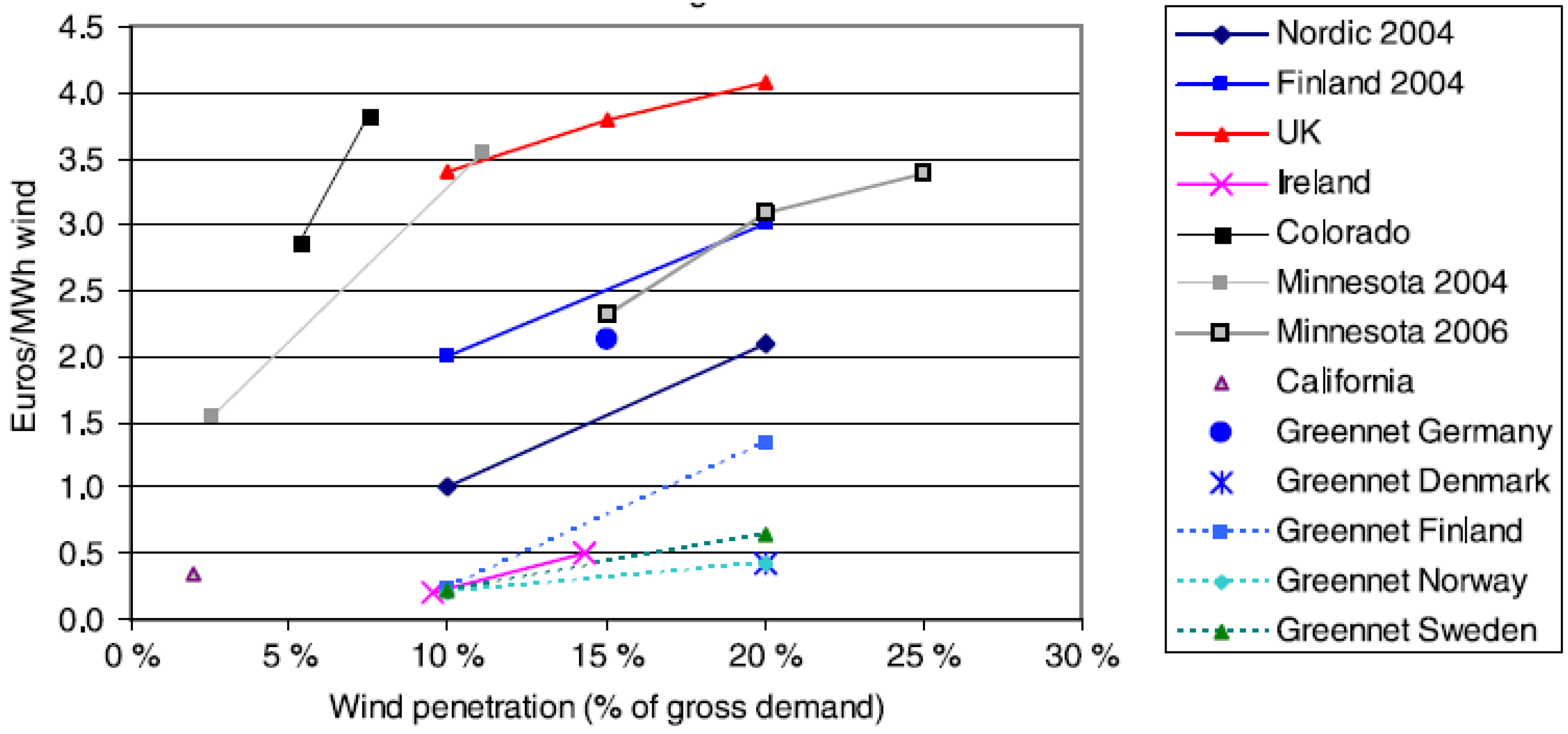
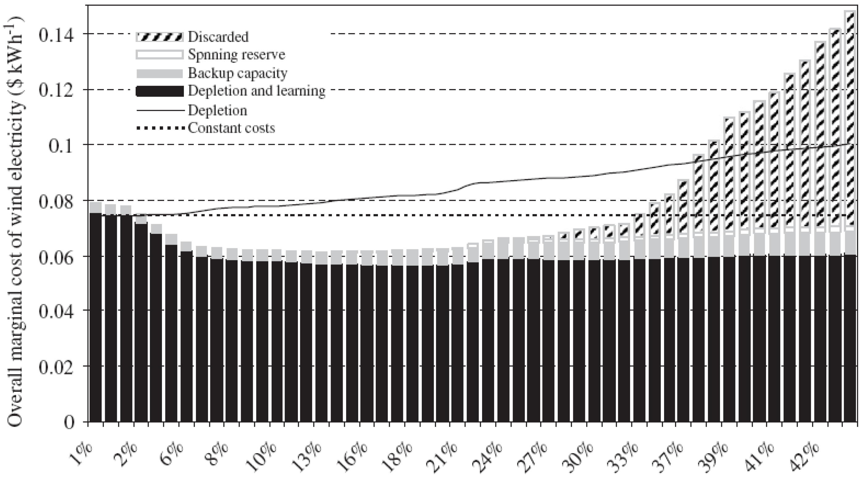
Hoogwijk, M.M.; Van Vuuren, D.; De Vries, B.J.M.; Turkenburg, W.C. Exploring the impact on cost and electricity production of high penetration levels of intermittent electricity in OECD Europe and the USA, results for wind energy. Energy 2007, 32, 1381–1402. [Google Scholar] [CrossRef]
Jha, A. Saharan sun to power European supergrid. The Guardian, 2008. [Google Scholar]
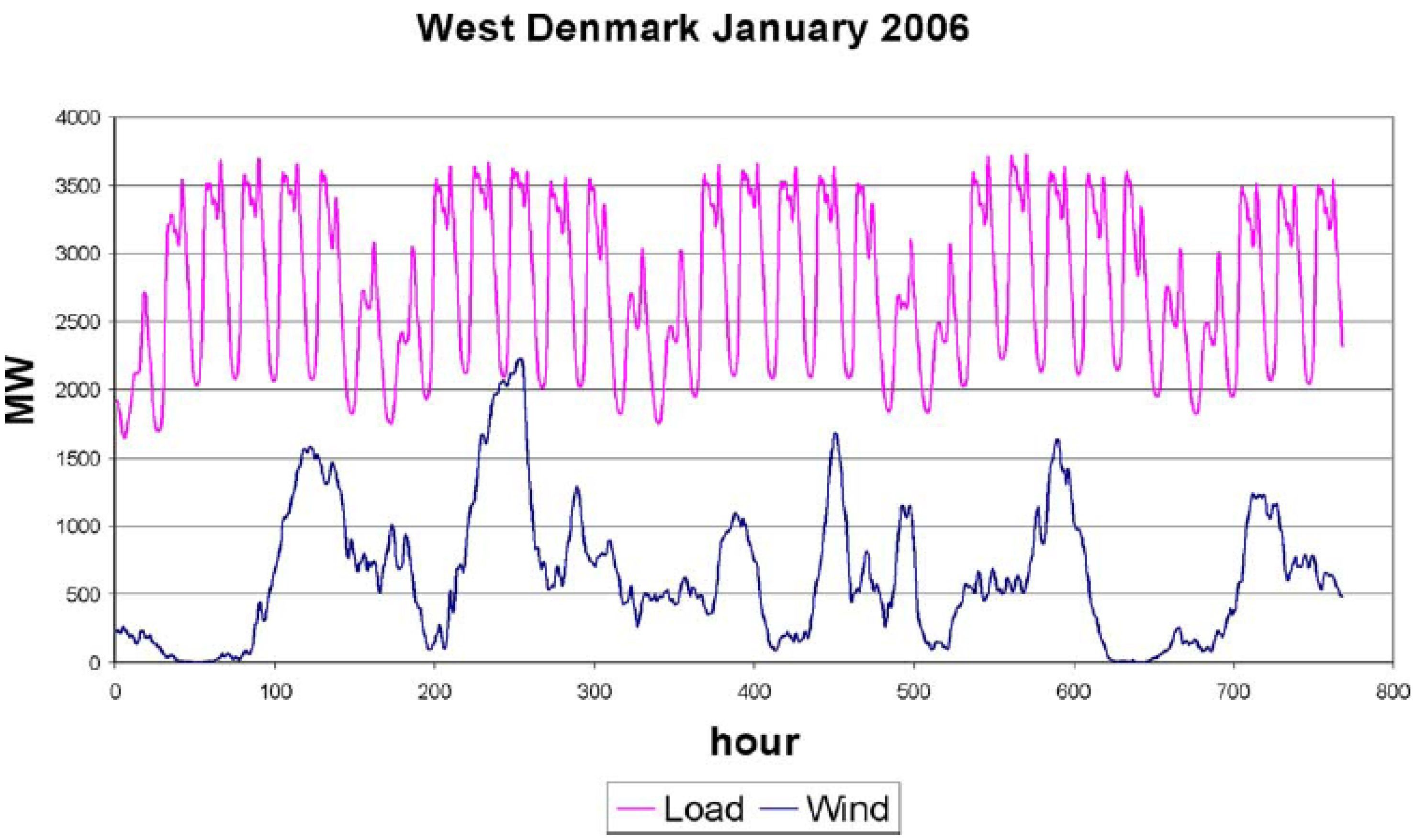
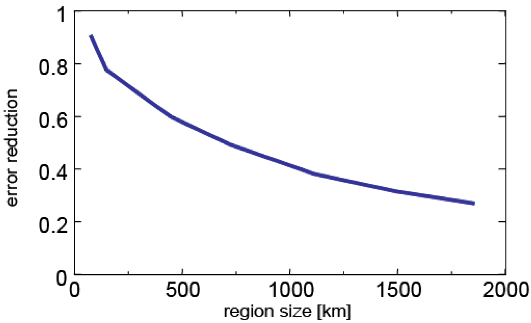
Østergaard, P.A. Geographic aggregation and wind power output variance in Denmark. Energy 2008, 33, 1453–1460. [Google Scholar] [CrossRef]
Schott AG. Memorandum on Solar Thermal Power Plant Technology; Schott AG: Mainz, Germany, 2005. [Google Scholar]
Cherigui, A.N.; Mahmah, B.; Harouadi, F.; Belhamel, M.; Chader, S.; M'Raoui, A.; Etievant, C. Solar hydrogen energy: The European-Maghreb connection. A new way of excellence for a sustainable energy development. Int. J. Hydrogen Energy 2009, 34, 4934–4940. [Google Scholar]
Global Wind Energy Outlook; Global Wind Energy Council: Brussels, Belgium, 2008.
Archer, C.L.; Jacobson, M.Z. Evaluation of global wind power. J. Geophys. Res. 2005, 110, D12110:1–D12110:20. [Google Scholar]
Hoogwijk, M.M.; De Vries, B.J.M.; Turkenburg, W.C. Assessment of the global and regional geographical, technical and economic potential of onshore wind energy. Energ. Econ. 2004, 26, 889–919. [Google Scholar] [CrossRef]
20% Wind Energy by 2030; DOE/GO-102008-2567; U.S. Department of Energy: Oak Ridge, USA, 2008.
Carolin Mabel, M.; Fernandez, E. Growth and future trends of wind energy in India. Renew. Sustain. Energy Rev. 2008, 12, 1745–1757. [Google Scholar] [CrossRef]
Xia, C.; Song, Z. Wind energy in China: Current scenario and future perspectives. Renew. Sustain. Energy Rev. 2009, 13, 1966–1974. [Google Scholar]
Kempton, W.; Archer, C.L.; Dhanju, A.; Garvine, R.W.; Jacobson, M.Z. Large CO₂ reductions via offshore wind power matched to inherent storage in energy end-uses. Geophys. Res. Lett. 2007, 34, L02817:1–L02817:5. [Google Scholar]
Snyder, B.; Kaiser, M.J. Ecological and economic cost-benefit analysis of offshore wind energy. Renewable Energy 2009, 34, 1567–1578. [Google Scholar] [CrossRef]
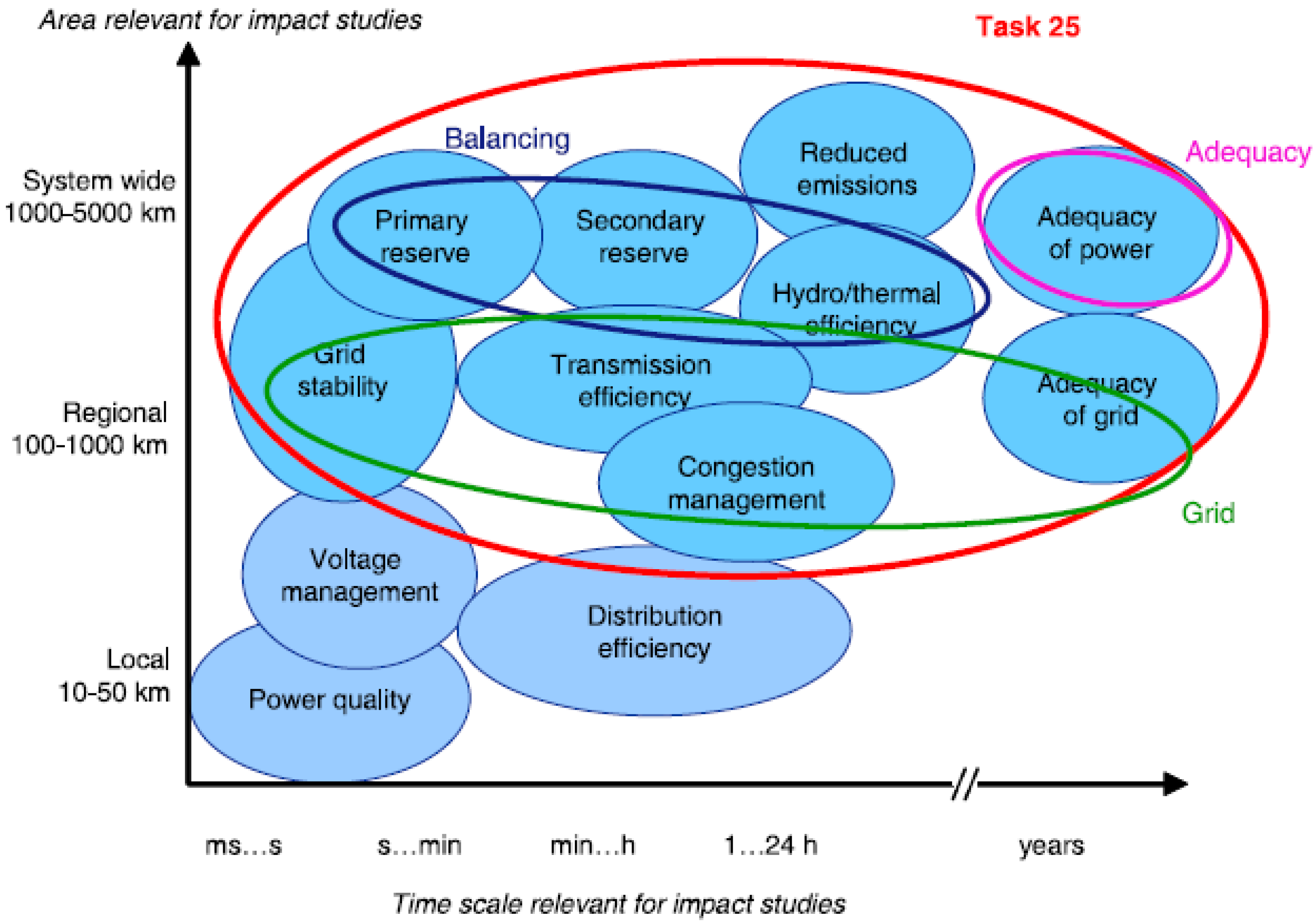
Holttinen, H. Estimating the impacts of wind power on power systems - summary of IEA Wind collaboration. Environ. Res. Lett. 2008, 3, 025001:1–025001:6. [Google Scholar] [CrossRef]
Resch, G.; Held, A.; Faber, T.; Panzer, C.; Toro, F.; Haas, R. Potentials and prospects for renewable energies at global scale. Energ. Policy 2008, 36, 4048–4056. [Google Scholar] [CrossRef]
Ackermann, T.; Söder, L. An overview of wind energy - status 2002. Renew. Sustain. Energy Rev. 2002, 6, 67–128. [Google Scholar] [CrossRef]
Archer, C.L.; Jacobson, M.Z. Supplying baseload power and reducing transmission requirements by interconnecting wind farms. J. Appl. Meteorol. Climatol. 2007, 46, 1701–1717. [Google Scholar] [CrossRef]
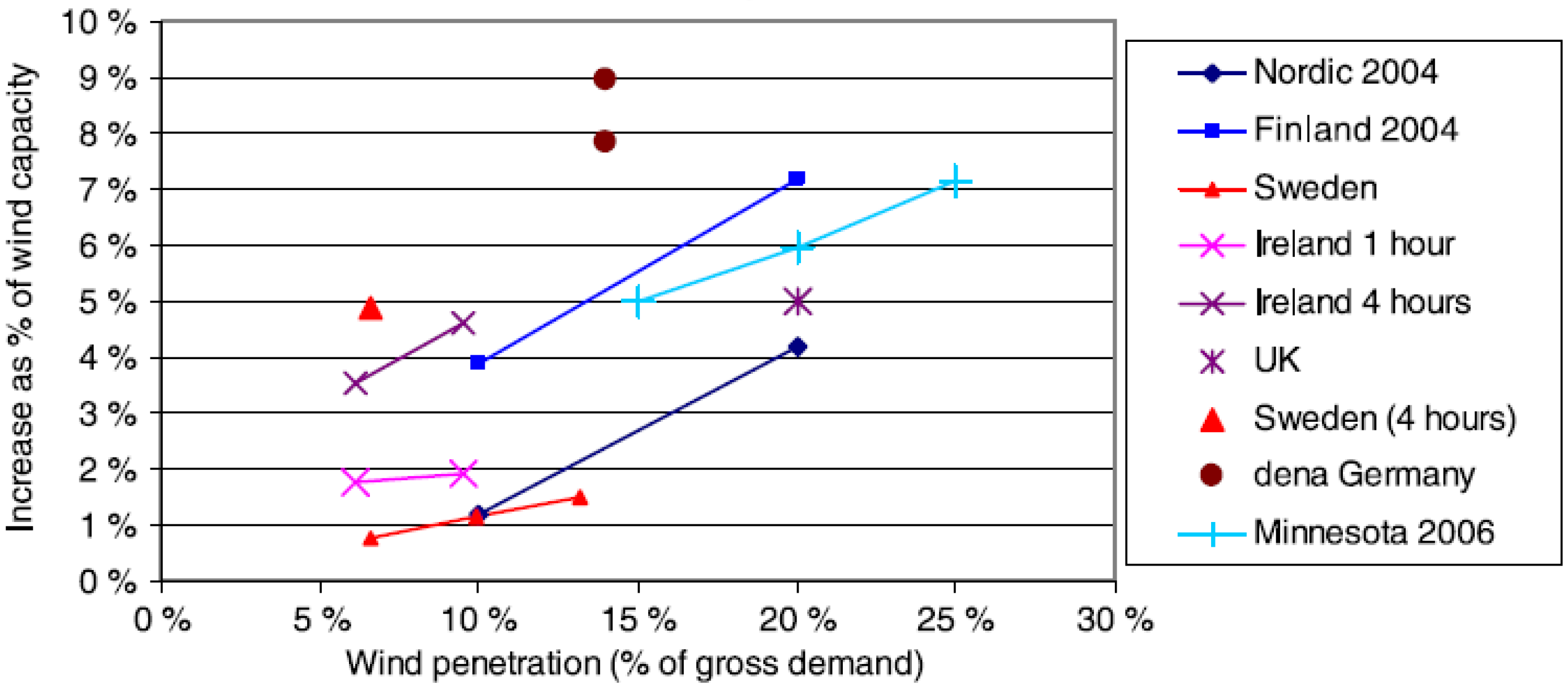
Holttinen, H.; Milligan, M.; Kirby, B.; Acker, T.; Neimane, V.; Molinski, T. Using standard deviation as a measure of increased operational reserve requirement for wind power. Wind Eng. 2008, 32, 355–378. [Google Scholar] [CrossRef]
Oswald, J.; Raine, M.; Ashraf-Ball, H. Will British weather provide reliable electricity? Energ. Policy 2008, 36, 3212–3225. [Google Scholar] [CrossRef]
Weigt, H. Germany’s wind energy: The potential for fossil capacity replacement and cost saving. Appl. Energ. 2008, 86, 1857–1863. [Google Scholar]
Holttinen, H.; Lemström, B.; Meibom, P.; Bindner, H.; Orths, A.; Van Hulle, F.; Ensslin, C.; Tiedemann, A.; Hofmann, L.; Winter, W.; Tuohy, A.; O'Malley, M.; Smith, P.; Pierik, J.; Tande, J.O.; Estanqueiro, A.; Ricardo, J.; Gomez, E.; Smith, J.C.; Söder, L.; Strbac, G.; Shakoor, A.; Smith, J.C.; Parsons, B.; Milligan, M.; Wan, Y.H. Design and operation of power systems with large amounts of wind power; VTT: Helsinki, Finland, 2007. [Google Scholar]
Archer, C.L.; Jacobson, M.Z. Spatial and temporal distributions of U.S. winds and wind power at 80 m derived from measurements. J. Geophys. Res. 2003, 108, 4289:1–4289:20. [Google Scholar]
Söder, L. On limits for wind power generation. Int. J. Global Energy Issue. 2004, 21, 243–254. [Google Scholar] [CrossRef]
Söder, L.; Hofmann, L.; Orths, A.; Holttinen, H.; Wan, Y.H.; Tuohy, A. Experience from wind integration in some high penetration areas. IEEE Trans. Energ. Conv. 2007, 22, 4–12. [Google Scholar]
Pavlak, A. The economic value of wind energy. Electricity J. 2008, 21, 46–50. [Google Scholar] [CrossRef]
Diesendorf, M. The Base-Load Fallacy; energyscience.org.au, 2007. [Google Scholar]
Holttinen, H.; Meibom, P.; Orths, A.; O'Malley, M.; Ummels, B.C.; Tande, J.O.; Estanqueiro, A.; Gomez, E.; Smith, J.C.; Ela, E. Impacts of large amounts of wind power on design and operation of power systems, results of IEA collaboration. Process of 7th International Workshop on Large Scale Integration of Wind Power and on Transmission Networks for Offshore Wind Farms; Madrid, Spain, 2008. Internet site http://windintegrationworkshop.org/previous_workshops.html.
Strbac, G.; Shakoor, A.; Black, M.; Pudjianto, D.; Bopp, T. Impact of wind generation on the operation and development of the UK electricity systems. Elec. Power Syst. Res. 2007, 77, 1214–1227. [Google Scholar] [CrossRef]
Martin, B.; Diesendorf, M. Calculating the capacity credit of wind power. In Fourth Biennial Conference of the Simulation Society of Australia; University of Queensland, 1980. [Google Scholar]
Milligan, M.; Porter, K. Determining the capacity value of wind: an updated survey of methods and implementation; NREL/CP-500-43433; National Renewable Energy Laboratory: Golden, USA, 2008. [Google Scholar]
DeCarolis, J.F.; Keith, D.W. The economics of large-scale wind power in a carbon constrained world. Energ. Policy 2006, 34, 395–410. [Google Scholar] [CrossRef]
Østergaard, P.A. Transmission grid requirements wit scattered and fluctuating renewable electricity-sources. Appl. Energ. 2003, 76, 247–255. [Google Scholar] [CrossRef]
Sovacool, B.K.; Lindboe, H.H.; Odgaard, O. Is the Danish wind energy model replicable for other countries? Electricity J. 2008, 21, 27–28. [Google Scholar] [CrossRef]
Lund, H. Large-scale integration of wind power into different energy systems. Energy 2005, 30, 2402–2412. [Google Scholar] [CrossRef]
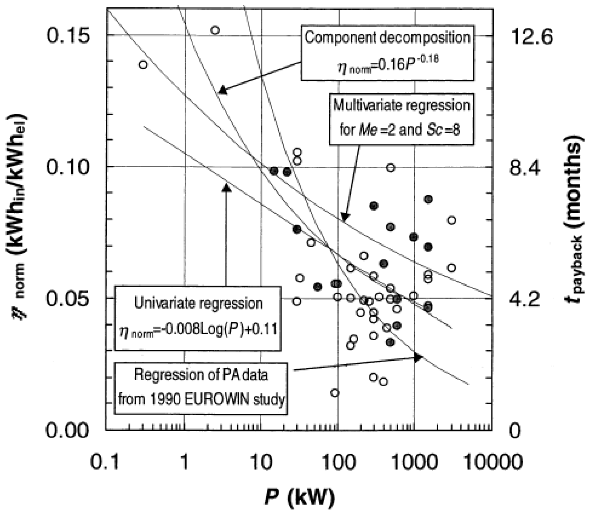
Wagner, H.J.; Pick, E. Energy yield ratio and cumulative energy demand for wind energy converters. Energy 2004, 29, 2289–2295. [Google Scholar] [CrossRef]
Pehnt, M.; Oeser, M.; Swider, D.J. Consequential environmental system analysis of expected offshore wind electricity production in Germany. Energy 2008, 33, 747–759. [Google Scholar] [CrossRef]
Jha, A. Brawny wind turbines set for German offshore debut. The Guardian Weekly, 2009; 10. [Google Scholar]
Joselin Herbert, G.M.; Iniyan, S.; Sreevalsan, E.; Rajapandian, S. A review of wind energy technologies. Renew. Sustain. Energy Rev. 2007, 11, 1117–1145. [Google Scholar] [CrossRef]
Bolinger, M.; Wiser, R. Wind power price trends in the United States: Struggling to remain competitive in the face of strong growth. Energ. Policy 2009, 37, 1061–1071. [Google Scholar] [CrossRef]
Wind; OECD/IEA: Paris, France, 2008.
Blanco, M.I. The economics of wind energy. Renew. Sustain. Energy Rev. 2008, 13, 1372–1382. [Google Scholar]
Welch, J.B.; Venkateswaran, A. The dual sustainability of wind energy. Renew. Sustain. Energy Rev. 2008, 13, 1121–1126. [Google Scholar]
Smit, T.; Junginger, M.; Smits, R. Technological learning in offshore wind energy: Different roles of the government. Energ. Policy 2007, 35, 6431–6444. [Google Scholar] [CrossRef]
Benitez, L.E.; Benitez, P.C.; Van Kooten, G.C. The economics of wind power with energy storage. Energ. Econ. 2008, 30, 1973–1989. [Google Scholar] [CrossRef]
Smith, J.C.; Milligan, M.; DeMeo, E.A.; Parsons, B. Utility wind integration and operating impact state of the art. IEEE Trans. Power Syst. 2007, 22, 900–908. [Google Scholar] [CrossRef]
Hirst, E.; Hild, J. The value of wind power as a function of wind capacity. Electricity J. 2004, 17, 11–20. [Google Scholar] [CrossRef]
Martin, B.; Diesendorf, M. Optimal mix in electricity grids containing wind power. Elec. Power Energ. Syst. 1982, 4, 155–161. [Google Scholar] [CrossRef]
Ilex, X.; Strbac, G. Quantifying the system cost of additional renewables in 2020; Ilex Energy Consulting: Oxford, UK, 2002. [Google Scholar]
Lund, H.; Kempton, W. Integration of renewable energy into the transport and electricity sectors through V2G. Energ. Policy 2008, 36, 3578–3587. [Google Scholar] [CrossRef]
Tavner, P. Wind power as a clean-energy contributor. Energ. Policy 2008, 36, 4397–4400. [Google Scholar] [CrossRef]
Zoellner, J.; Schweizer-Ries, P.; Wemheuer, C. Public acceptance of renewable energies: Results from case studies in Germany. Energ. Policy 2008, 36, 4136–4141. [Google Scholar] [CrossRef]
Kurokawa, K.; Komoto, K.; van der Vleuten, P.; Faiman, D. Energy from the Desert-Practical proposals for Very Large Scale Photovoltaic Systems; Earthscan: London, UK, 2006. [Google Scholar]
Ito, M.; Kato, K.; Sugihara, H.; Kichimi, T.; Song, J.; Kurokawa, K. A preliminary study on potential for very large-scale photovoltaic power generation (VLS-PV) system in the Gobi desert from economic and environmental viewpoints. Solar Energ. Mater. Solar Cells 2003, 75, 507–517. [Google Scholar] [CrossRef]
Zweibel, K.; Mason, J.; Fthenakis, V.M. A solar grand plan. Sci. Amer. 2008, 298, 64–73. [Google Scholar] [CrossRef] [PubMed]
Trevisani, L.; Fabbri, M.; Negrini, F. Long-term scenarios for energy and environment: Energy from the desert with very large solar plants using liquid hydrogen and superconducting technologies. Fuel Process. Technol. 2006, 87, 157–161. [Google Scholar] [CrossRef]
Global Market Outlook for Photovoltaics until 2012; European Photovoltaic Industry Association: Brussels, Belgium, 2008.
IEA, Healthy markets, but room for improvement. PV Power, 2008; 4–5.
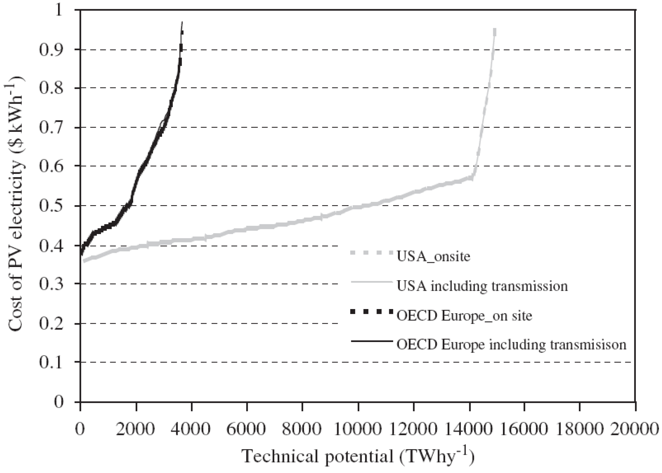
Fthenakis, V.; Mason, J.E.; Zweibel, K. The technical, geographical, and economic feasibility for solar energy to supply the energy needs of the US. Energ. Policy 2009, 37, 387–399. [Google Scholar] [CrossRef]
Raugei, M.; Frankl, P. Life cycle impacts and costs of photovoltaic systems: Current state of art and future outlooks. Energy 2009, 34, 392–399. [Google Scholar] [CrossRef]
Hoffmann, W. PV solar electricity industry: Market growth and perspective. Solar Energ. Mater. Solar Cells 2006, 90, 3285–3311. [Google Scholar] [CrossRef]
PV snapshot; www.iea-pvps.orgInternational Energy Agency: Paris, France, 2009.
Perez, R.; Margolis, R.; Kmiecik, M.; Schwab, M.; Perez, M. Update: Effective Load-Carrying Capacity of photovoltaics in the United States; NREL/CP-620-40068; National Renewable Energy Laboratory: Springfield, USA, 2006. [Google Scholar]
Rüther, R.; Knob, P.J.; da Silva Jardim, C.; Rebechi, S.H. Potential of building integrated photovoltaic solar energy generators in assisting daytime peaking feeders in urban areas in Brazil. Energ. Conv. Manage. 2008, 49, 1074–1079. [Google Scholar] [CrossRef]
Pelland, S.; Abboud, I. Comparing photovoltaic capacity value metrics: a case study of the City of Toronto. Prog. Photovoltaics 2008, 16, 715–724. [Google Scholar] [CrossRef]
Herig, C. Using Photovoltaics to Preserve California's Electricity Capacity Reserves; NREL/BR-520-31179; National Renewable Energy Laboratory: Springfield, USA, 2001. [Google Scholar]
Crawford, R.; Treloar, G.; Fuller, R.; Bazilian, M. Life-cycle energy analysis of building integrated photovoltaic systems (BiPVs) with heat recovery unit. Renew. Sustain. Energy Rev. 2006, 10, 559–575. [Google Scholar] [CrossRef]
Fthenakis, V.M.; Kim, H.C. CdTe photovoltaics: Life cycle environmental profile and comparisons. Thin Solid Films 2007, 515, 5961–5963. [Google Scholar] [CrossRef]
Celik, A.N.; Muneer, T.; Clarke, P. A review of installed solar photovoltaic and thermal collector capacities in relation to solar potential for the EU-15. Renewable Energy 2009, 34, 849–856. [Google Scholar] [CrossRef]
Liu, L.; Wang, Z. The development and application practice of wind-solar energy hybrid generation systems in China. Renew. Sustain. Energy Rev. 2008, 13, 1504–1512. [Google Scholar]
IEA, PV industry landscape becoming truly global. PV Power, 2008; 2–3.
Bagnall, D.M.; Boreland, M. Photovoltaic technologies. Energ. Policy 2008, 36, 4390–4396. [Google Scholar] [CrossRef]
Mondol, J.D.; Yohanis, Y.G.; Norton, B. Optimising the economic viability of grid-connected photovoltaic systems. Appl. Energ. 2009, 86, 985–999. [Google Scholar] [CrossRef]
Mehos, M. Task I: Solar Thermal Electric Systems; www.solarpaces.org/Tasks/Task1/task_i.htmNational Renewable Energy Laboratories, 2007.
Trieb, F.; Nitsch, J.; Kronshage, S.; Schillings, C.; Brischke, L.-A.; Knies, G.; Czisch, G. Combined solar power and desalination plants for the Mediterranean region-sustainable energy supply using large-scale solar thermal power plants. Desalination 2002, 153, 39–46. [Google Scholar] [CrossRef]
Morse, F.H. The Global Market Initiative (GMI) for Concentrating Solar Power (CSP). In ASES Conference; Portland, USA, 2004. [Google Scholar]
Brakmann, G.; Aringhoff, R.; Geyer, M.; Teske, S. Concentrated Solar Power; www.solarpaces.org/Library/CSP_Documents/Concentrated-Solar-Thermal-Power-Plants-2005.pdfEuropean Solar Thermal Industry Association: Birmingham, UK, 2005.
DLR. European Concentrated Solar Thermal Road-Mapping; SES6-CT-2003-502578; Deutsches Zentrum für Luft- und Raumfahrt e.V.: Köln, Germany, 2005. [Google Scholar]
Aringhoff, R.; Geyer, M.; Morse, F.H. The Concentrating Solar Power Global Market Initiative; http://www.solarpaces.org/_Libary/GMI_10.pdfEuropean Solar Thermal Power Industry Association, IEA SolarPACES, and U.S. Solar Energy Industry Associations: Washington D.C., USA, 2004.
Trieb, F. Competitive solar thermal power stations until 2010-the challenge of market introduction. Renewable Energy 2000, 19, 163–171. [Google Scholar] [CrossRef]
Concentrating Solar Power for the Mediterranean region; Deutsches Zentrum für Luft- und Raumfahrt e.V.: Stuttgart, Germany, 2005.
Broesamle, H.; Mannstein, H.; Schillings, C.; Trieb, F. Assessment of solar electricity potentials in North Africa based on satellite data and a geographic information system. Solar Energ. 2001, 70, 1–12. [Google Scholar] [CrossRef]
Ummel, K.; Wheeler, D. Desert Power: The Economics of Solar Thermal Electricity for Europe, North Africa, and the Middle East; 156; Center for Global Development: Washington D.C., USA, 2008. [Google Scholar]
Lovegrove, K.; Luzzi, A. Solar Thermal Power Systems. In Encyclopedia of Physical Science and Technology; 2002; Vol. 15, pp. 223–235. [Google Scholar]
Montes, M.J.; Abánades, A.; Martínez-Val, J.M. Performance of a direct steam generation solar thermal power plant for electricity production as a function of the solar multiple. Solar Energ. 2008, 679, 679–689. [Google Scholar]
Concentrated Solar Thermal Energy; Directorate J-Energy-European Commission: Luxembourg, Luxembourg, 2004.
Kaneff, S. Solar thermal process heat and electricity generation performance and costs for the ANU 'Big Dish' technology - a comparison with LUZ system costs; EP-RR-57; Energy Research Centre, Research School of Physical Sciences & Engineering, Institute of Advanced Studies, The Australian National University: Canberra, Australia, April 1992. [Google Scholar]
Pilkington. Status report on solar trough power plants; Pilkington Solar International GmbH: Köln, Germany, 1996. [Google Scholar]
Mills, D.R.; Morrison, G.L. Compact Linear Fresnel Reflector solar thermal powerplants. Solar Energ. 2000, 68, 263–283. [Google Scholar] [CrossRef]
Mills, D. Advances in solar thermal electricity technology. Solar Energ. 2004, 76, 19–31. [Google Scholar] [CrossRef]
Schramek, P.; Mills, D.R. Multi-tower solar array. Solar Energ. 2003, 75, 249–260. [Google Scholar] [CrossRef]
Schramek, P.; Mills, D.R. Heliostats for maximum ground coverage. Energy 2004, 29, 701–713. [Google Scholar] [CrossRef]
Trieb, F. Concentrating Solar Power for Europe, Middle East and North Africa – A roadmap to 2050. In Hannover Messe; Hannover, Germany, 2007. [Google Scholar]
Trieb, F.; Müller-Steinhagen, H. Concentrating solar power for seawater desalination in the Middle East and North Africa. Desalination 2008, 220, 165–183. [Google Scholar] [CrossRef]
Trieb, F.; Müller-Steinhagen, H.; Kern, J.; Scharfe, J.; Kabariti, M.; Al Taher, A. Technologies for large scale seawater desalination using concentrated solar radiation. Desalination 2009, 235, 33–43. [Google Scholar] [CrossRef]
Solar Millennium. The Parabolic Trough Power Plants Andasol 1 to 3; Solar Millennium AG: Erlangen, Germany, 2009. [Google Scholar]
Lenzen, M.; Treloar, G. Differential convergence of life-cycle inventories towards upstream production layers. J. Ind. Ecol. 2003, 6, 137–160. [Google Scholar] [CrossRef]
Caldés, N.; Varela, M.; Santamaría, M.; Sáez, R. Economic impact of solar thermal electricity deployment. Energ. Policy 2009, 37, 1628–1636. [Google Scholar] [CrossRef]
Lenzen, M.; Dey, C.J. Economic, energy and emissions impacts of some environmentally motivated consumer, technology and government spending options. Energ. Econ. 2002, 24, 377–403. [Google Scholar] [CrossRef]
Dey, C.; Mills, D.R.; Morrison, G.L. Operation of a CLFR research apparatus. In ANZSES Annual Conference; Geelong, Australia, 1999. [Google Scholar]
Concentrating Solar Power - from research to implementation; European Commission: Luxembourg, Luxembourg, 2007.
Tsoutsous, T.; Gekas, V.; Marketaki, K. Technical and economical evaluation of solar thermal power generation. Renewable Energy 2003, 28, 873–886. [Google Scholar] [CrossRef]
Beerbaum, S.; Weinrebe, G. Solar thermal power generation in India - a techno-economic analysis. Renewable Energy 2000, 21, 153–174. [Google Scholar] [CrossRef]
Quaschning, V. Technical and economical system comparison of photovoltaic and concentrating solar thermal power systems depending on annual global irradiation. Solar Energ. 2004, 77, 171–178. [Google Scholar] [CrossRef]
Assessment of Parabolic Trough and Power Tower Solar Technology Cost and Performance Forecasts; LAA-2-32458-01; Sargent & Lundy LLC Consulting Group; NREL/SR-550-34440; National Renewable Energy Laboratory: Golden, USA, 2003.
Lovegrove, K.; Luzzi, A.; Soldiani, I.; Kreetz, H. Developing ammonia based thermochemical energy storage for dish power plants. Solar Energ. 2004, 76, 331–337. [Google Scholar] [CrossRef]
Dahl, J.K.; Buechler, K.J.; Finley, R.; Stanislaus, T.; Weimer, A.W.; Lewandowski, A.; Bingham, C.; Smeets, A.; Schneider, A. Rapid solar-thermal dissociation of natural gas in an aerosol flow reactor. Energy 2004, 29, 715–725. [Google Scholar] [CrossRef]
Kodama, T. High-temperature solar chemistry for converting solar heat to chemical fuels. Prog. Energ. Combust. Sci. 2003, 29, 567–597. [Google Scholar] [CrossRef]
Lodhi, M.A.K. Helio-hydro and helio-thermal production of hydrogen. Int. J. Hydrogen Energy 2004, 29, 1099–1113. [Google Scholar]
Stein, W. Solar Thermal Project; www.det.csiro.au/science/r_h/solarthermal.htmCSIRO: Canberra, Australia, 2005.
DiPippo, R. Geothermal Power Generating Systems. In Geothermal Power Plants (Second Edition); Butterworth-Heinemann: Oxford, 2008; pp. 79–80. [Google Scholar]
DiPippo, R. Worldwide State of Geothermal Power Plant Development as of May 2007. In Geothermal Power Plants (Second Edition); Butterworth-Heinemann: Oxford, 2008; pp. 413–432. [Google Scholar]
MIT. The Future of Geothermal Energy; Massachusetts Institute of Technology: Boston, USA, 2006. [Google Scholar]
Blodgett, L.; Slack, K. Geothermal 101: Basics of Geothermal Energy Production and Use; Geothermal Energy Association: Washington, USA, 2009. [Google Scholar]
Taylor, M.A. The State of Geothermal Technology; Geothermal Energy Association: Washington, USA, 2007. [Google Scholar]
DiPippo, R. Binary Cycle Power Plants. In Geothermal Power Plants (Second Edition); Butterworth-Heinemann: Oxford, 2008; pp. 157–189. [Google Scholar]
DiPippo, R. Single-Flash Steam Power Plants. In Geothermal Power Plants (Second Edition); Butterworth-Heinemann: Oxford, 2008; pp. 81–112. [Google Scholar]
DiPippo, R. Double-Flash Steam Power Plants. In Geothermal Power Plants (Second Edition); Butterworth-Heinemann: Oxford, 2008; pp. 113–133. [Google Scholar]
DiPippo, R. Dry-Steam Power Plants. In Geothermal Power Plants (Second Edition); Butterworth-Heinemann: Oxford, 2008; pp. 135–156. [Google Scholar]
Bertani, R. World geothermal power generation in the period 2001-2005. Geothermics 2005, 34, 651–690. [Google Scholar] [CrossRef]
Dickson, M.H.; Fanelli, M. What is Geothermal Energy? http://www.geothermal-energy.org/geo/geoenergy.phpIstituto di Geoscienze e Georisorse: Pisa, Italy, 2004.
DiPippo, R. Environmental Impact of Geothermal Power Plants. In Geothermal Power Plants (Second Edition); Butterworth-Heinemann: Oxford, 2008; pp. 385–410. [Google Scholar]
Imroz Sohel, M.; Sellier, M.; Brackney, L.J.; Krumdieck, S. Efficiency improvement for geothermal power generation to meet summer peak demand. Energ. Policy 2009, 37, 3370–3376. [Google Scholar] [CrossRef]
Sanner, B.; Bussmann, W. Current status, prospects and economic framework of geothermal power production in Germany. Geothermics 2003, 32, 429–438. [Google Scholar] [CrossRef]
Stefánsson, V. Investment cost for geothermal power plants. Geothermics 2002, 31, 263–272. [Google Scholar] [CrossRef]
Gawell, K.; Greenberg, G. Update on world geothermal development; http://www.geo-energy.org/publications/reports/GEA%20World%20Update%202007.pdfGeothermal Energy Association: Washington, DC, USA, 2007.
Kagel, A.; Bates, D.; Gawell, K. A guide to geothermal energy and the environment; Geothermal Energy Association: Washington D.C., USA, 2007. [Google Scholar]
DiPippo, R. The Geysers Dry-Steam Power Plants, Sonoma and Lake Counties, California, U.S.A. In Geothermal Power Plants (Second Edition); Butterworth-Heinemann: Oxford, 2008; pp. 277–297. [Google Scholar]
IGA. Installed Generating Capacity; http://www.geothermal-energy.org/geoworld/geoworld.php?sub=elgenInternational Geothermal Association: Reykjavik, Iceland, 2009.
GEA. Factors affecting costs of geothermal power development; Geothermal Energy Association: Washington D.C., USA, 2005. [Google Scholar]
Hansson, J.; Berndes, G.; Johnsson, F.; Kjärstad, J. Co-firing biomass with coal for electricity generation--An assessment of the potential in EU27. Energ. Policy 2009, 37, 1444–1455. [Google Scholar] [CrossRef]
Taylor, G. Biofuels and the biorefinery concept. Energ. Policy 2008, 36, 4406–4409. [Google Scholar] [CrossRef]
Gokcol, C.; Dursun, B.; Alboyaci, B.; Sunan, E. Importance of biomass energy as alternative to other sources in Turkey. Energ. Policy 2009, 37, 424–431. [Google Scholar] [CrossRef]
Siriwardhana, M.; Opathella, G.K.C.; Jha, M.K. Bio-diesel: Initiatives, potential and prospects in Thailand: A review. Energ. Policy 2009, 37, 554–559. [Google Scholar] [CrossRef]
UN-Energy. Sustainable Bioenergy: A Framework for Decision-Makers; http://esa.un.org/un-energy/pdf/susdev.Biofuels.FAO.pdfUnited Nations: New York, USA, 2007.
Righelato, R.; Spracklen, D.V. Carbon Mitigation by Biofuels or by Saving and Restoring Forests? Science 2007, 318, 902. [Google Scholar] [PubMed]
Nonhebel, S. Energy from agricultural residues and consequences for land requirements for food production. Agr. Syst. 2007, 94, 586–592. [Google Scholar] [CrossRef]
Lal, R. Land area for establishing biofuel plantations. Energ. Sustain. Dev. 2006, 10, 67–79. [Google Scholar] [CrossRef]
Sims, R.E.H.; Taylor, M.; Saddler, J.; Mabee, W. From 1^st- to 2^nd-Generation Biofuel Technologies; International Energy Agency: Paris, France, 2008. [Google Scholar]
Goldemberg, J.; Guardabassi, P. Are biofuels a feasible option? Energ. Policy 2009, 37, 10–14. [Google Scholar] [CrossRef]
Demirbas, A. Biofuels sources, biofuel policy, biofuel economy and global biofuel projections. Energ. Conv. Manage. 2008, 49, 2106–2116. [Google Scholar] [CrossRef]
Field, C.B.; Campbell, J.E.; Lobell, D.B. Biomass energy: the scale of the potential resource. Trend. Ecol. Evolut. 2008, 23, 65–72. [Google Scholar] [CrossRef]
Perlack, R.D.; Wright, L.L.; Turhollow, A.F.; Graham, R.L.; Stokes, B.J.; Erbach, D.C. Biomass as a feedstock for a bioenergy and bioproducts industry: The technical feasibility of a billion-ton annual supply; US Department of Energy, US Department of Agriculture: Oak Ridge, USA, 2005.
Haq, Z. Biomass for electricity generation. http://www.eia.doe.gov/oiaf/analysispaper/biomass/pdf/biomass.pdfU.S. Department of Energy, Energy Information Administration: Washington D.C., USA, 2003.
Knight, B.; Westwood, A. World biomass review: Biomass as a global power source. Refocus 2004, 5, 42–44. [Google Scholar] [CrossRef]
Hoogwijk, M.; Faaij, A.; de Vries, B.; Turkenburg, W. Exploration of regional and global cost-supply curves of biomass energy from short-rotation crops at abandoned cropland and rest land under four IPCC SRES land-use scenarios. Biomass Bioenerg. 2009, 33, 26–43. [Google Scholar] [CrossRef]
Hoogwijk, M.; Faaij, A.; Eickhout, B.; de Vries, B.; Turkenburg, W. Potential of biomass energy out to 2100, for four IPCC SRES land-use scenarios. Biomass Bioenerg. 2005, 29, 225–257. [Google Scholar] [CrossRef]
Smeets, E.; Faaij, A.P.C.; Lewandowski, I. A quickscan of global bio-energy potentials to 2050; NWS-E-2004-109; Copernicus Institute - Department of Science, Technology and Society: Utrecht University, Netherlands, 2004. [Google Scholar]
Hoogwijk, M.; Faaij, A.; van den Broek, R.; Berndes, G.; Gielen, D.; Turkenburg, W. Exploration of the ranges of the global potential of biomass for energy. Biomass Bioenerg. 2003, 25, 119–133. [Google Scholar] [CrossRef]
Moore, R.B. Algal Biofuels Industry. Adelaide, Australia, 2009. [Google Scholar]
Kelly-Yong, T.L.; Lee, K.T.; Mohamed, A.R.; Bhatia, S. Potential of hydrogen from oil palm biomass as a source of renewable energy worldwide. Energ. Policy 2007, 35, 5692–5701. [Google Scholar] [CrossRef]
Thornley, P.; Upham, P.; Huang, Y.; Rezvani, S.; Brammer, J.; Rogers, J. Integrated assessment of bioelectricity technology options. Energ. Policy 2009, 37, 890–903. [Google Scholar] [CrossRef]
Soimakallio, S.; Mäkinen, T.; Ekholm, T.; Pahkala, K.; Mikkola, H.; Paappanen, T. Greenhouse gas balances of transportation biofuels, electricity and heat generation in Finland—Dealing with the uncertainties. Energ. Policy 2009, 37, 80–90. [Google Scholar] [CrossRef]
Su, C.-L.; Lee, Y.-M. Development status and life cycle inventory analysis of biofuels in Taiwan. Energ. Policy 2009, 37, 754–758. [Google Scholar] [CrossRef]
Searchinger, T.; Heimlich, R.; Houghton, R.H.; Dong, F.; Elobeid, A.; Fabiosa, J.; Togkoz, S.; Hayes, D.; Yu, T. Use of US croplands for biofuels increases greenhouse gases through emissions from land use change. Science 2008, 319, 1238–1240. [Google Scholar]
Fargione, J.; Hill, J.; Tilman, D.; Polasky, S.; Hawthorne, P. Land clearing and the biofuel carbon debt. Science 2008, 319, 1235–1238. [Google Scholar] [CrossRef] [PubMed]
Wicke, B.; Dornburg, V.; Junginger, M.; Faaij, A. Different palm oil production systems for energy purposes and their greenhouse gas implications. Biomass Bioenerg. 2008, 32, 1322–1337. [Google Scholar] [CrossRef]
Foran, B.; Lenzen, M.; Dey, C. Balancing Act - A Triple Bottom Line Account of the Australian Economy; http://www.isa.org.usyd.edu.auCSIRO Resource Futures and The University of Sydney: Canberra, ACT, Australia, 2005.
Gagnon, L.; Bélanger, C.; Uchiyama, Y. Life-cycle assessment of electricity generation options: The status of research in 2001. Energ. Policy 2002, 30, 1267–1278. [Google Scholar] [CrossRef]
Ovando, P.; Caparrós, A. Land use and carbon mitigation in Europe: A survey of the potentials of different alternatives. Energ. Policy 2009, 37, 992–1003. [Google Scholar] [CrossRef]
Fthenakis, V.; Kim, H.C. Land use and electricity generation: A life-cycle analysis. Renew. Sustain. Energy Rev. 2009, 13, 1465–1474. [Google Scholar] [CrossRef]
Thornley, P.; Rogers, J.; Huang, Y. Quantification of employment from biomass power plants. Renewable Energy 2008, 33, 1922–1927. [Google Scholar] [CrossRef]
Skytte, K.; Meibom, P.; Henriksen, T.C. Electricity from biomass in the European union-With or without biomass import. Biomass Bioenerg. 2006, 30, 385–392. [Google Scholar] [CrossRef]
Münster, M.; Lund, H. Use of waste for heat, electricity and transport—Challenges when performing energy system analysis. Energy 2009, 34, 636–644. [Google Scholar] [CrossRef]
Altman, I.; Johnson, T. Organization of the current U.S. biopower industry: A template for future bioenergy industries. Biomass Bioenerg 2009, 33, 779–784. [Google Scholar] [CrossRef]
De, S.; Assadi, M. Impact of cofiring biomass with coal in power plants-A techno-economic assessment. Biomass Bioenerg. 2009, 33, 283–293. [Google Scholar] [CrossRef]
Gan, J.; Smith, C.T. A comparative analysis of woody biomass and coal for electricity generation under various CO2 emission reductions and taxes. Biomass Bioenerg. 2006, 30, 296–303. [Google Scholar] [CrossRef]
United Nations, Soaring biofuel demand driving up agricultural prices, says UN-backed report. UN News, 2007.
Wang, L.; Weller, C.L.; Jones, D.D.; Hanna, M.A. Contemporary issues in thermal gasification of biomass and its application to electricity and fuel production. Biomass Bioenerg. 2008, 32, 573–581. [Google Scholar] [CrossRef]
Fowler, P.; Krajačić, G.; Lončar, D.; Duić, N. Modeling the energy potential of biomass-H2RES. Int. J. Hydrogen Energy 2009, 34, 7027–7040. [Google Scholar] [CrossRef]
Yin, C.; Rosendahl, L.A.; Kær, S.K. Grate-firing of biomass for heat and power production. Prog. Energ. Combust. Sci. 2008, 34, 725–754. [Google Scholar] [CrossRef]
Taylor, G. Bioenergy for heat and electricity in the UK: A research atlas and roadmap. Energ. Policy 2008, 36, 4383–4389. [Google Scholar] [CrossRef]
Bunn, M.; Malin, M.B. Enabling a nuclear revival – and managing its risks. Innovations 2009, 4, 173–191. [Google Scholar] [CrossRef]

© 2010 by the authors; licensee Molecular Diversity Preservation International, Basel, Switzerland. This article is an open-access article distributed under the terms and conditions of the Creative Commons Attribution license (http://creativecommons.org/licenses/by/3.0/).

Share and Cite

MDPI and ACS Style

Lenzen, M. Current State of Development of Electricity-Generating Technologies: A Literature Review. Energies 2010, 3, 462-591. https://doi.org/10.3390/en3030462

AMA Style

Lenzen M. Current State of Development of Electricity-Generating Technologies: A Literature Review. Energies. 2010; 3(3):462-591. https://doi.org/10.3390/en3030462

Chicago/Turabian Style

Lenzen, Manfred. 2010. "Current State of Development of Electricity-Generating Technologies: A Literature Review" Energies 3, no. 3: 462-591. https://doi.org/10.3390/en3030462

Article Menu

Current State of Development of Electricity-Generating Technologies: A Literature Review

Abstract

1. Summary

2. Rationale

3. Introduction

3.1. Role of Electricity in World Energy Needs

3.2. Demand Projections and Scenarios

4. Carbon Capture and Storage

4.1. Potential of Resource

4.2. Post-combustion Capture

4.2.1. Technical principle

4.2.2. Capacity and load characteristics

4.2.3. Life-cycle characteristics

4.2.4. Current scale of deployment

4.2.5. Cost of electricity output

4.2.6. Technical challenges

4.3. Pre-combustion Capture

4.3.1. Technical principle

4.3.2. Capacity and load characteristics

4.3.3. Life-cycle characteristics

4.3.4. Current scale of deployment

4.3.5. Cost of electricity output

4.3.6. Technical challenges

4.4. Oxyfuel capture

4.4.1. Technical principle

4.4.2. Capacity and load characteristics

4.4.3. Life-cycle characteristics

4.4.4. Current scale of deployment

4.4.5. Cost of electricity output

4.4.6. Technical challenges

4.5. Geological Storage

4.5.1. Technical principle

4.5.2. Capacity and load characteristics

4.5.3. Life-cycle characteristics

4.5.4. Current scale of deployment

4.5.5. Contribution to global electricity supply

4.5.6. Cost of electricity output

2.1.1. Technical challenges

5. Nuclear Fission

5.1. Summary

5.2. Global potential of resource

5.3. Generation-II and -III reactors

5.3.1. Technical principle

5.3.2. Capacity and load characteristics

5.3.3. Life-cycle characteristics

5.3.4. Current scale of deployment

5.3.5. Contribution to global electricity supply

5.3.6. Cost of electricity output

5.3.7. Technical challenges

5.4. Generation-IV reactors

5.4.1. Technical principle

5.4.1.1. Breeding

5.4.1.2. Fast reactors

5.4.1.3. Fast and thermal breeder reactors

5.4.1.4. High burnup

5.4.1.5. Passive safety–The pebble bed and molten salt reactors

5.4.1.6. High-temperature heat – nuclear hydrogen

5.4.1.7. Thorium fuel cycle

5.4.1.8. Subcritical reactors

5.4.1.9. Transmutation

5.4.2. Capacity and load characteristics

5.4.3. Life-cycle characteristics

5.4.4. Current scale of deployment

5.4.5. Contribution to global electricity supply

5.4.6. Cost of electricity output

5.4.7. Technical challenges

6. Hydroelectric Power

6.1. Summary

6.2. Global Potential of Resource

6.3. Dam and run-of-river plants

6.3.1. Technical principle

6.3.2. Capacity and load characteristics

6.3.3. Life-cycle characteristics

6.3.4. Current scale of deployment

6.3.5. Contribution to global electricity supply

6.3.6. Cost of electricity output

6.3.7. Technical and other challenges

7. Wind energy

7.1. Summary