Forecasting Monthly Electric Energy Consumption Using Feature Extraction

Abstract

Monthly forecasting of electric energy consumption is important for planning the generation and distribution of power utilities. However, the features of this time series are so complex that directly modeling is difficult. Three kinds of relatively simple series can be derived when a discrete wavelet transform is used to extract the raw features, namely, the rising trend, periodic waves, and stochastic series. After the elimination of the stochastic series, the rising trend and periodic waves were modeled separately by a grey model and radio basis function neural networks. Adding the forecasting values of each model can yield the forecasting results for monthly electricity consumption. The grey model has a good capability for simulating any smoothing convex trend. In addition, this model can mitigate minor stochastic effects on the rising trend. The extracted periodic wave series, which contain relatively less information and comprise simple regular waves, can improve the generalization capability of neural networks. The case study on electric energy consumption in China shows that the proposed method is better than those traditionally used in terms of both forecasting precision and expected risk.

1. Introduction

Monthly forecasting of electric energy consumption plays an important role in the operation of thermal power plants and is one of the most important basis for coal dispatch, electricity trading, and so on. In addition, monthly forecasting of electric energy consumption is vital for the planning and maintenance of the grid. However, a number of difficulties are associated with forecasting. First, the steady monthly consumption trends of electric energy often change every few years as a result of macroeconomic conditions and social development. Therefore, the data used for modeling can only be derived from a continuous number of years, during which macroeconomic conditions may have varied slightly. Second, the monthly consumption trend data is extremely complex because of the effects of people’s living habits, weather conditions, and other unexpected factors. Thus, the monthly consumption trends often comprise at least three kinds of sub-trends, namely, a long-term rising trend, numerous periodical waves, and the stochastic series.

Classical techniques, such as regression [1] and expert systems [2], are incapable of generating precise forecasting results because of low adaptability. On the other hand, time series methods [3,4,5] use a moving average to simplify the raw trends. These methods remove tiny waves to smoothen the data figures. As a result, time series methods have been proven to be better than classical techniques. However, the primary limitation of these methods is the inability to distinguish stochastic waves from a number of other useful waves. As a result, useful information may be mistakenly eliminated and the forecasting results of these methods are often unsatisfactory because not all the useful information in the raw data is considered.

In the past several years, neural networks (NNs) have been widely applied in short-term load forecasting (STLF) [6,7,8,9,10] and short-term price forecasting [11,12]. The primary advantage of a NN is its capability for modeling non-linear relations without the supervision of human experts [13,14]. When used for load forecasting, NNs require significant volumes of data for training [15], while requiring relatively less information from each sample (the relationship between input and output vectors is relatively simple). These factors are important for forecasting precision, however, based on the aforementioned reasons, collecting adequate steady monthly data, even for the short term, is difficult. Furthermore, compared with short-term load data (e.g., 96-point daily ones), monthly data often contain more information. To date, although NN has been widely used for monthly data forecasting, its applications are limited to either special trends [16] or special points (e.g., peak load prediction) [17].

The key to further improvement of the forecasting precision of NN in monthly forecasting is the reduction of the amount of information in each sample. In fact, sample simplification is also a feasible method for STLF [6]. For monthly forecasting, feature extraction is an effective method for reducing the amount of information in each sample. Zhao and Wei [18] have summarized a number of methods for extracting the series features. González–Romera et al. [19,20,21] adopted a moving average algorithm to extract the rising trend from a monthly electric energy demand series. The width of the data window in the moving average is selected by measuring the fitting accuracy and the smoothness of the obtained rising figure. The periodic wave is forecasted using the Fourier series, whereas the rising trend is predicted by NNs. The extracting techniques, combined with other methods, were proven to be capable of yielding better forecasting results compared with the time series and single NN methods.

However, the previously designed models were still observed to have certain limitations. First, the Fourier series can only simulate waves with invariable amplitude. However, the amplitude of periodic waves extracted from the raw trends will inevitably increase because of rapid increases in total monthly electric energy consumption, especially in developing countries. Second, the moving average method is only capable of separating waves from the rising trend, but is incapable of eliminating the stochastic effect. Third, the use of NNs to simulate the extracted rising trend cannot easily mitigate minor unexpected factors (e.g., the continuous occurrence of freak weather), thereby affecting generalizability.

The present paper adopts a discrete wavelet transform (DWT) to decompose the raw forecasting figure. DWT is not only capable of extracting the rising trend and periodic waves, but it can also distinguish stochastic behavior. Periodic waves are forecasted by NNs, which can simulate their increasing amplitude. As a feasible method for simulating convex function, the grey model (GM) is adopted to forecast the rising trend.

The paper is structured as follows: Section 2 briefly introduces the principles and primary algorithms used in the present work. Section 3 presents the case study on the monthly electric energy consumption in China as an example to test the model. Aside from the forecasting method discussed in Section 2, two other transitional methods are designed to test the contribution of each innovation, and both methods are compared with the traditional algorithm through forecasting error analysis. Section 4 concludes the present paper.

2. Feature Extraction and Forecasting Algorithms

2.1. Feature Extraction Based on DWT

As a time-frequency decomposition method for a discrete signal, DWT is used in the present work with the aim of decomposing the monthly time series. The DWT function ψ_j,k(t) can be written as:

$${\psi }_{j,k}(t)=a^{-j/2}\psi \left(\frac{t-k{a}^{j}b}{a^j}\right)=a^{-j/2}\psi (a^{-j}t-kb)$$

(1)

where a^j is a scale function and ka^jb is a translation function, both of which are derived from a continuous wavelet transform (CWT) by discreteness.

For any discrete function f(t), the discrete wavelet coefficient C_j,k is derived from:

$$C_{j,k}={\displaystyle {\int }_{-\infty }^{+\infty }f(t){\psi }_{j,k}^{*}(t)dt}$$

(2)

where * denotes the complex conjugation of ψ. The discrete wavelet coefficient can be used to reconstruct the function f(t) as follows:

$$f(t)=C{\displaystyle \sum _{j=-\infty }^{\infty }{\displaystyle \sum _{k=-\infty }^{\infty }{C}_{j,k}{\psi }_{j,k}(t)}}$$

(3)

where C is a constant. A schematic diagram of the DWT process is shown in Figure 1.

Figure 1. Multi-resolution analysis using DWT.

Figure 1. Multi-resolution analysis using DWT.

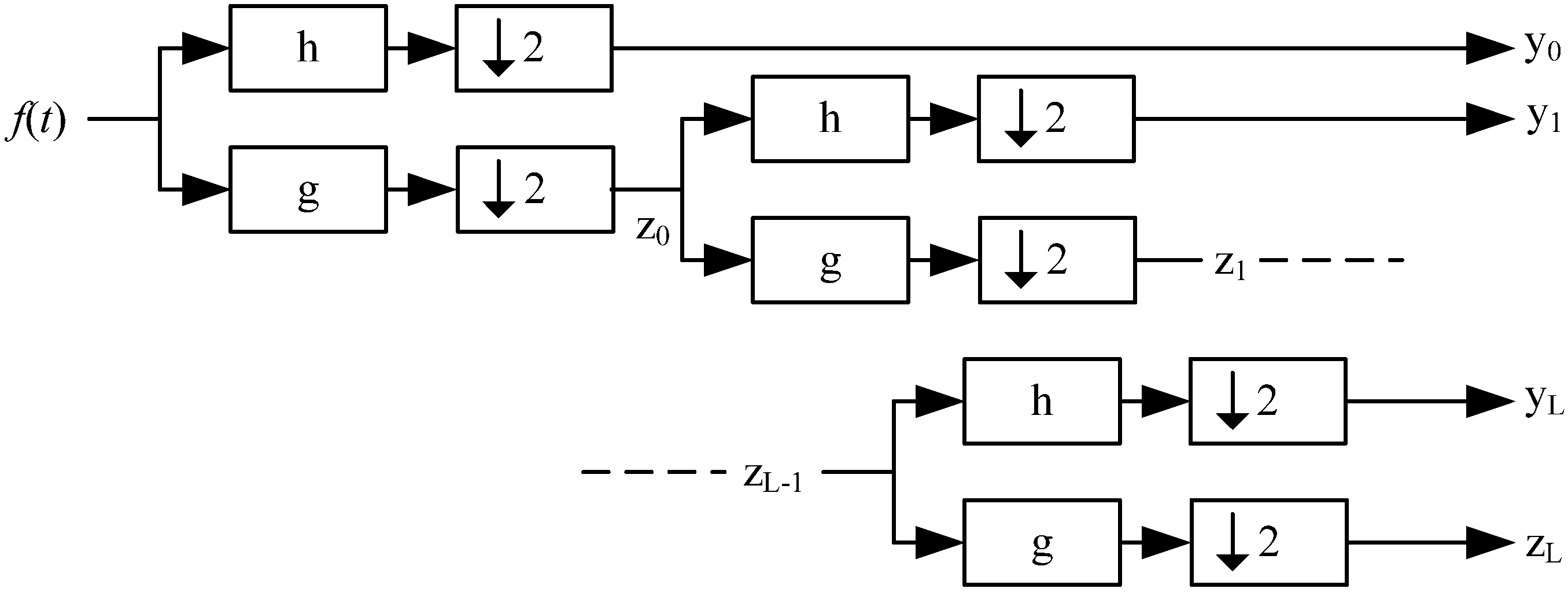
The DWT decomposes a signal into low-frequency (z_L) and high-frequency coefficients (y₀ − y_L). The low-frequency and high-frequency coefficients comprise the approximate features and the details of f(t), respectively. The relationship between these values is defined by f(t) = z_L + y₀ + y₁ + … + y_L.

For a wavelet function, Daubechies wavelets were selected for extracting the features of the monthly electric energy consumption series. These wavelets are an orthogonal family defining a discrete wavelet transform and are characterized by a maximal number of vanishing moments for a given support [22].

2.2. GM for Exponential Trend Forecasting

If the socio-economy runs smoothly, both the economic growth rate and electric elasticity coefficient tend to be constant. As a result, the reconstructed result of low frequency extracted from the monthly electric energy consumption series using DTW has a steadily increasing trend, which can be simulated using the following equation:

$$x=b_1+b_2\exp (b_{3}t)$$

(4)

where b₁, b₂, and b₃ are the shape parameters. In fact, by adjusting the parameters of b₁, b₂, and b₃, Equation (4) can simulate any smoothing convex trend. The optimum parameters of Equation (4) cannot be obtained by minimizing the residual sum of square (RSS) because of the location of b₃. Deng [23,24] proposed a method for solving this problem.

The following differential form of Equation (4) can be processed to obtain the optimum parameters of a and u by minimizing the RSS:

$$\frac{dx}{dt}+ax=u$$

(5)

To process the discrete series, Equation (5) should be discretized as follows:

$$x^{(0)}(k+1)+\frac{1}{2}a[x^{(1)}(k+1)+x^{(1)}(k)]=u$$

(6)

where x⁽⁰⁾(k) (k = 1,2,…) refers to the raw series, and x⁽¹⁾(k) (k = 1,2,…) stands for the accumulated generating series and is written as $x^{(1)}(k)={\displaystyle \sum _{i=1}^k{x}^{(0)}(i)}$.

Integrating the raw and the accumulated generating series with the iterative Equation (6) will yield the following:

$$N=B\cdot A$$

(7)

where N = [x⁽⁰⁾ (2) x⁽⁰⁾ (3) … x⁽⁰⁾ (n)]^T, A = [a u]^T, and $B=\left[\begin{array}{cc}-\frac{1}{2}[x^{(1)}(1)+x^{(1)}(2)]& 1\\ -\frac{1}{2}[x^{(1)}(2)+x^{(1)}(3)]& 1\\ ⋮& ⋮\\ -\frac{1}{2}[x^{(1)}(n-1)+x^{(1)}(n)]& 1\end{array}\right]$

The RSS can then be minimized to obtain the optimum parameters of Equation (5):

$$\min ||N-B\cdot \widehat{A}||=\min {(N-B\cdot \widehat{A})}^{\mathrm{T}}(N-B\cdot \widehat{A})$$

(8)

Using a matrix derivative will yield:

$$\widehat{A}={(B^{\mathrm{T}}B)}^{-1}{B}^{\mathrm{T}}N={[\begin{array}{cc}\widehat{a}& \widehat{u}\end{array}]}^{\mathrm{T}}$$

(9)

Using the optimum parameters obtained in Equation (9) and adopting x⁽¹⁾(1) as a particular solution will yield the following solution for Equation (5):

$$x^{(1)}(k+1)=[x^{(0)}(1)-\frac{\widehat{u}}{\widehat{a}}]\exp (-\widehat{a}k)+\frac{\widehat{u}}{\widehat{a}}$$

(10)

Through inverse accumulated generating operation, the forecasting model of x⁽⁰⁾ is derived as follows:

$$x^{(0)}(k+1)=(1-\exp (\widehat{a}))(x^{(0)}(1)-\frac{\widehat{u}}{\widehat{a}})\exp (-\widehat{a}k)$$

(11)

where k = 0,1,2,….

In Equation (11), k is the only variable. The forecasting value is obtained only by entering an appropriate k. Considering the characteristics of Equation (11) k should equal i − 1 when forecasting the ith value.

2.3. RBF NNs for Periodical Waves

In 1988, Broomhead and Lowe introduced the radial basis function (RBF) to the NN field. As a classic multilayer feedforward NN, the RBF NN often consists of three layers, namely, the input, the hidden, and the output layers. The input layer gathers the input vector x, whereas the output layer yields the output vector y. According to the Kolmogorov theorem, given any n-dimension continuous mapping f, U × U…… × U → R × R…… × R, where f(x) = y and U $\in$ [0, 1], f can be simulated using a three-layer feedforward NN. For any nonlinear fluctuant, a three-layer feedforward NN can be used for theoretical simulation at any precision.

Unlike other feedforward NNs, the kernel function of an RBF NN is a Gauss function that is usually written as:

$$u_j=\text{exp}\left[-\frac{{(x-w_j)}^{\mathrm{T}}(x-w_j)}{2{\sigma }_j^2}\right], j=1,2,\dots ,{\mathrm{N}}_1$$

(12)

where u_j is the output value of jth node in the hidden layer, x is the input vector of the hidden layer, w_j is the center of the Gauss function of the jth node, σ_j² is the spread of the Gauss function, and N₁ is the number of nodes in the hidden layer. Based on Equation (12), the output of each Gauss function will be between 0 and 1. Furthermore, each Gauss function has a reflection (significantly unequal 0) only when the input vector is very close to the space center (w_j).

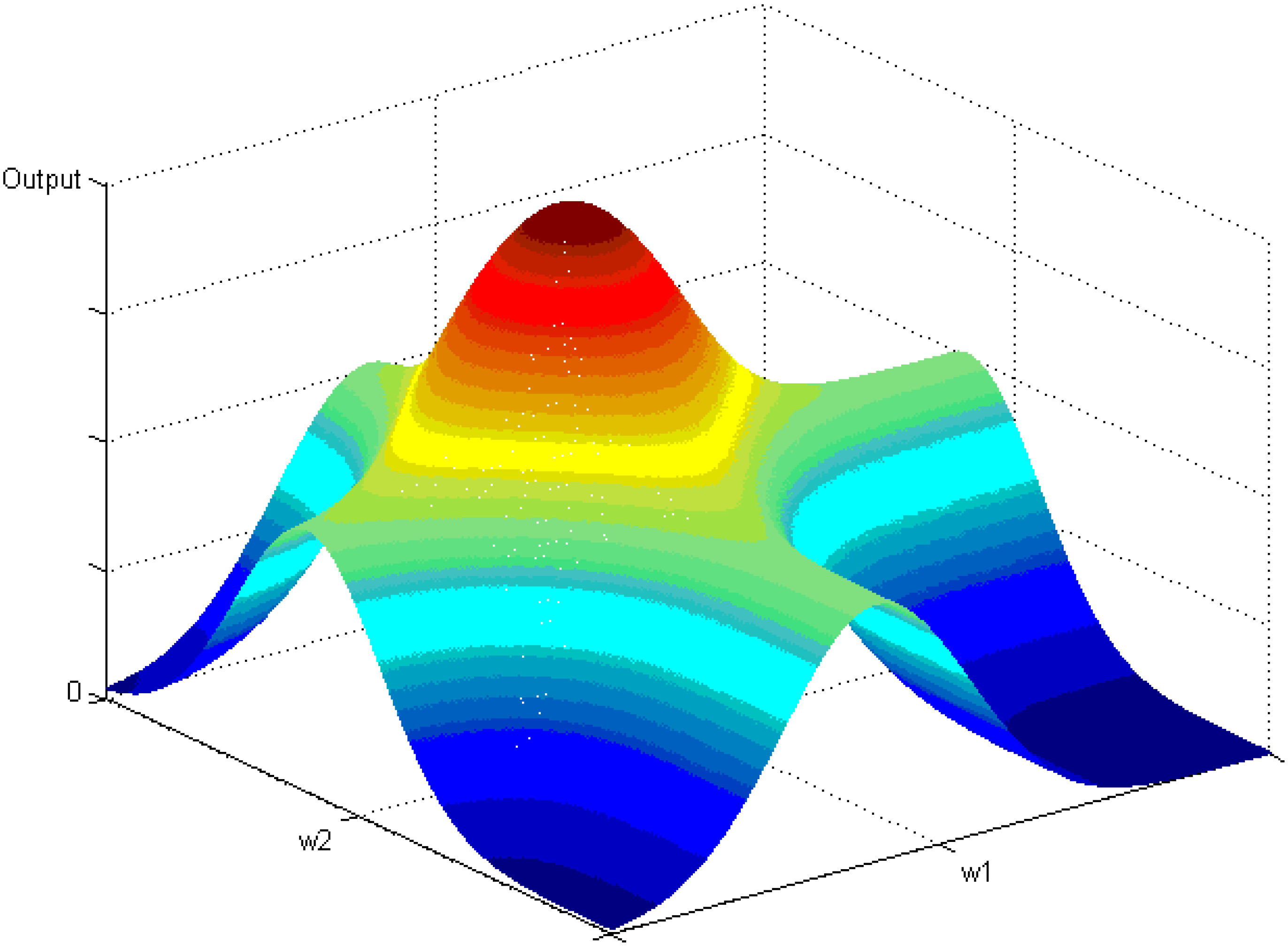
Figure 2 shows the output distribution of the RBF NN with two Gauss function nodes. The output of the RBF NN is clearly seen to rapidly approach 0 when the inputs deviate from the centers.

Figure 2. Outputs of RBF NN with two nodes in the hidden layer.

Figure 2. Outputs of RBF NN with two nodes in the hidden layer.

For high-dimension input vectors, the RBF NN has better learning efficiency compared with the traditional error back propagation NN, which adopts an S-like kernel function that has reflections in infinite space. That is, the RBF NN often has a rapid convergence rate and enhanced training speed, which are very important because NNs will be frequently utilized in the proposed forecasting model.

2.4. Forecasting Model Design

The operation of the monthly electric energy consumption forecasting model involves the following steps: first, the historical data are decomposed by DWT and then reconstructed by each frequency. Reconstructed results with a small amplitude and an indistinct wave period (considered as stochastic waves) are eliminated; second, the rising trend (the reconstructed result of low-frequency) is modeled using GM (1, 1), and other periodical waves (the remaining reconstructed results from different high frequencies) are determined using the RBF NNs; third, the forecasting results of monthly electric energy consumption are obtained by adding the forecasting values of the previous models. The next section will demonstrate the forecasting steps in detail.

3. Experimental Setup and Forecasting Results

The actual values of the monthly electric energy consumption (10⁸ kWh) in China from January 1990 to December 2006 were selected to validate the aforementioned methods. Data were obtained from the website of the Chinese Economic and Financial Database of the China Center for Economic Research (CCER) [25]. The monthly electric energy consumption curve (Figure 3) obviously exhibits a basic exponential rising trend and is characterized by numerous waves.

Figure 3. Monthly electricity consumption in China from January 1990 to December 2006.

Figure 3. Monthly electricity consumption in China from January 1990 to December 2006.

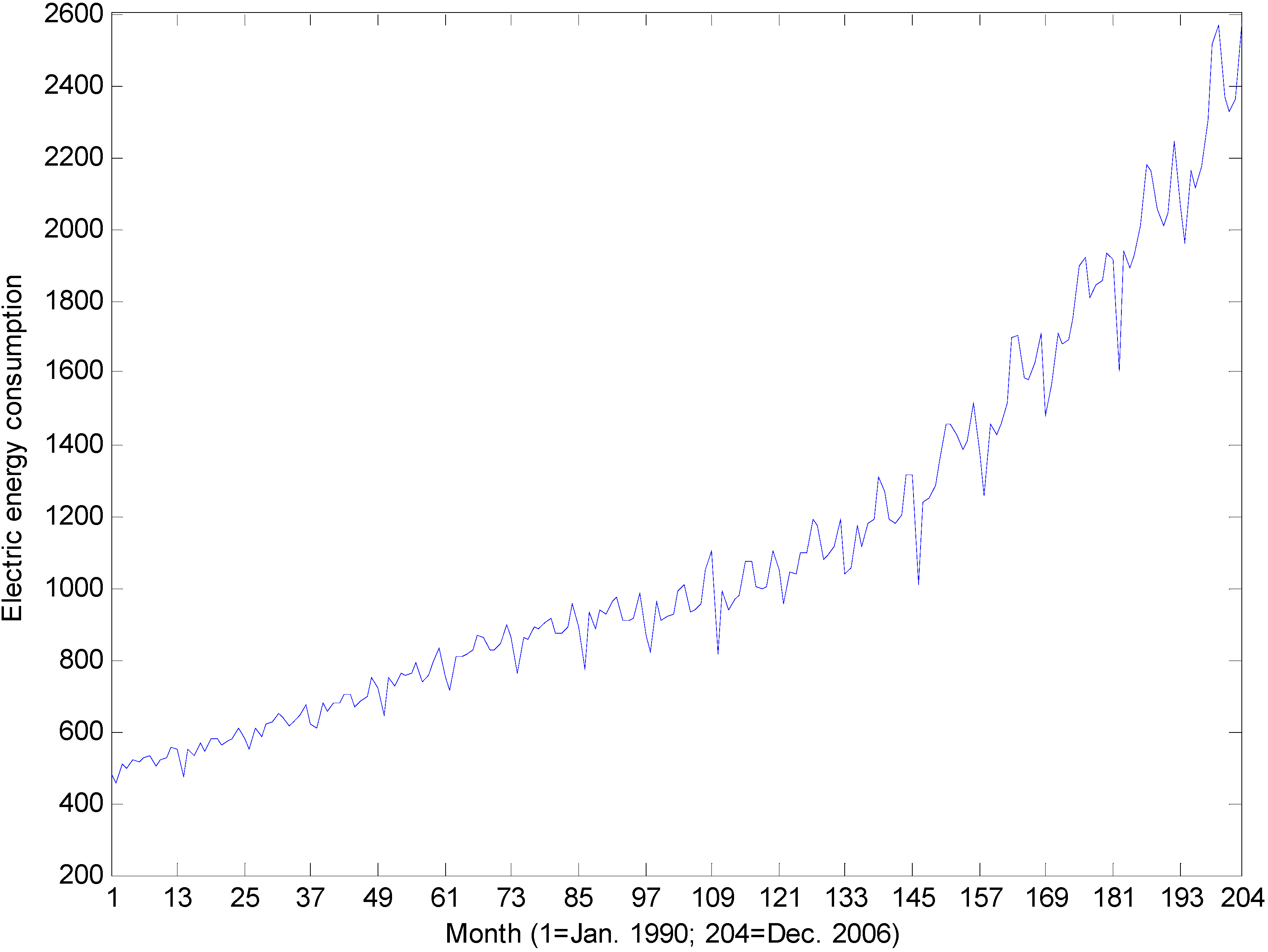
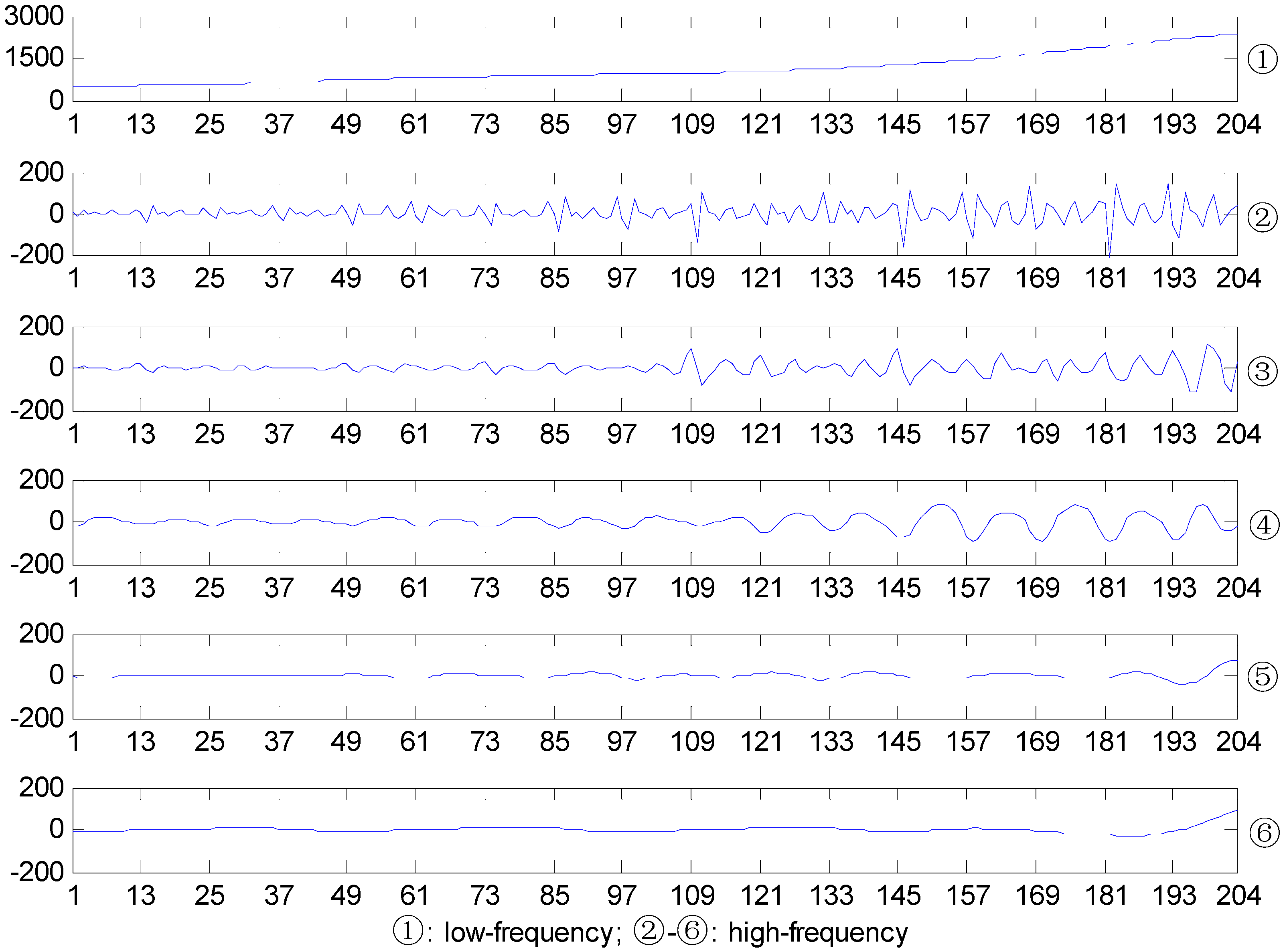
Figure 3 was decomposed using the db(5) wavelet and was further reconstructed by each frequency. The reconstructed results of each frequency are shown in Figure 4.

The reconstructed low-frequency Result (1) reflects the primary monthly electric energy consumption trend, which exhibits an exponential rise. Results (2)–(4) reflect periodical waves of different frequencies. Amplitudes were observed to gradually increase with the development of the social economy. Results (5) and (6) have no distinct wave periods, and their amplitudes were generally very small. Thus, these results were classified as stochastic waves and consequently eliminated. In fact, the summation of Results (1)–(4) is 98.4% similar to the actual data.

Figure 4. Results of db(5) wavelet transformation.

Figure 4. Results of db(5) wavelet transformation.

For the extracted rising trend, the reconstructed low-frequency result has been modeled using GM (1, 1). For each forecasting point, 12 consecutive previously obtained values have been adopted to model the exponential forecasting equation. The trend value of forecasting was derived assuming k = 12 in Equation (11).

For the reserved reconstructed high-frequency results (Results (2)–(4) in Figure 4), RBF NN has been adopted to simulate the relationship between the current and a number of its previous values. For each forecasting point, 60 of its consecutive previous values were selected for RBF NN training. The 13th to 60th values were taken as outputs. For each output value, 12 previous values were selected as the inputs. After training, the NN is used for forecasting. Based on the same rule, when forecasting the jth point, the 12 consecutive previous values are entered and the output of NN is considered the forecasting result. For example, if the value of certain remaining reconstructed results of January 2005 were to be forecasted, the values from January 2000 to December 2004 from the same time series were selected to establish the NN structure. When constructing training samples, the values from January 2001 to December 2004 were successively selected as outputs, and the 12 previous values of each of these outputs were selected as the inputs.

In the current paper, all RBF NNs were implemented using the Matlab Neural Network Toolbox and were designed to have similar parameters, i.e., the neuron number of the RBF layer refers to the dimension of the input vector and the training goal defaults to 0. Furthermore, the value of spread will greatly affect the feature of RBF. The larger that spread is the smoother the function approximation will be. Here it is set at 50. After the NN structures were established, the values from January to December of 2004 were used as the inputs for the network. The consequent output was the forecasting result of January 2005.

The forecasting values of GM and RBF NNs were combined to yield the forecasted results of monthly electric energy consumption in China (hereinafter Method 1). The forecasting results and errors from January 2005 to December 2006 are listed in Table 1.

Table 1. Analysis of forecasting results.

	Actual Data	Method 1	Error (%)	Method 2	Error (%)	Method 3	Error (%)	Method 4	Error (%)
Jan. 2005	1914.89	1934.16	1.01	1811.98	5.37	1797.75	−6.12	1931.2	0.85
Feb.	1601.06	1686.78	5.35	1770.77	−10.6	1741.73	8.79	1684.61	5.22
Mar.	1940.47	1879.17	−3.16	1912.86	1.42	1893.04	−2.44	1877.78	−3.23
Apr.	1892.06	1843.68	−2.56	1906.05	−0.74	1878.43	−0.72	1843.17	−2.58
May	1924.7	1957.53	1.71	1950.29	−1.33	1907.51	−0.89	1957.53	1.71
Jun.	2006.75	2075.33	3.42	2006.39	0.02	1962.02	−2.23	2074.67	3.38
Jul.	2178.9	2148.25	−1.41	2160.61	0.84	2096.35	−3.79	2146.74	−1.48
Aug.	2162.05	2124.62	−1.73	2158.88	0.15	2092.78	−3.2	2122.05	−1.85
Sep.	2053.25	2035.17	−0.88	2083.3	−1.46	2018.1	−1.71	2031.7	−1.05
Oct.	2010.97	1916.54	−4.7	2093.51	−4.1	2024.17	0.66	1912.9	−4.88
Nov.	2041.89	1970.19	−3.51	2130.93	−4.36	2052	0.5	1966.37	−3.7
Dec.	2246.59	2195.55	−2.27	2250.09	−0.16	2145.64	−4.49	2191.91	−2.43
Jan. 2006	2063.39	2107.82	2.15	2057.61	0.28	2049.61	−0.67	2104.61	2
Feb.	1962.01	1990.85	1.47	1954.98	0.36	1927.18	−1.78	1988	1.32
Mar.	2161.62	2128.15	−1.55	2160.16	0.07	2137.9	−1.1	2125.66	−1.66
Apr.	2116.6	2059.6	−2.69	2137.18	−0.97	2114.38	−0.1	2057.53	−2.79
May	2175.28	2165.91	−0.43	2172.42	0.13	2153.48	−1	2164.19	−0.51
Jun.	2301.93	2289.92	−0.52	2228.76	3.18	2215.43	−3.76	2287.68	−0.62
Jul.	2517.14	2422.73	−3.75	2370.46	5.83	2368.84	−5.89	2419.8	−3.87
Aug.	2570.49	2468.77	−3.96	2361.52	8.13	2371.35	−7.75	2465.09	−4.1
Sep.	2364.75	2426.81	2.62	2258.85	4.48	2288.2	−3.24	2422.4	2.44
Oct.	2324.3	2300.76	−1.01	2266.56	2.48	2308.43	−0.68	2296.04	−1.22
Nov.	2363.36	2199.24	−6.94	2298.88	2.73	2346.64	−0.71	2194.15	−7.16
Dec.	2573.4	2439.59	−5.2	2391.33	7.08	2462.79	−4.3	2434.3	−5.41

Table 1. Analysis of forecasting results.

	Actual Data	Method 1	Error (%)	Method 2	Error (%)	Method 3	Error (%)	Method 4	Error (%)
Jan. 2005	1914.89	1934.16	1.01	1811.98	5.37	1797.75	−6.12	1931.2	0.85
Feb.	1601.06	1686.78	5.35	1770.77	−10.6	1741.73	8.79	1684.61	5.22
Mar.	1940.47	1879.17	−3.16	1912.86	1.42	1893.04	−2.44	1877.78	−3.23
Apr.	1892.06	1843.68	−2.56	1906.05	−0.74	1878.43	−0.72	1843.17	−2.58
May	1924.7	1957.53	1.71	1950.29	−1.33	1907.51	−0.89	1957.53	1.71
Jun.	2006.75	2075.33	3.42	2006.39	0.02	1962.02	−2.23	2074.67	3.38
Jul.	2178.9	2148.25	−1.41	2160.61	0.84	2096.35	−3.79	2146.74	−1.48
Aug.	2162.05	2124.62	−1.73	2158.88	0.15	2092.78	−3.2	2122.05	−1.85
Sep.	2053.25	2035.17	−0.88	2083.3	−1.46	2018.1	−1.71	2031.7	−1.05
Oct.	2010.97	1916.54	−4.7	2093.51	−4.1	2024.17	0.66	1912.9	−4.88
Nov.	2041.89	1970.19	−3.51	2130.93	−4.36	2052	0.5	1966.37	−3.7
Dec.	2246.59	2195.55	−2.27	2250.09	−0.16	2145.64	−4.49	2191.91	−2.43
Jan. 2006	2063.39	2107.82	2.15	2057.61	0.28	2049.61	−0.67	2104.61	2
Feb.	1962.01	1990.85	1.47	1954.98	0.36	1927.18	−1.78	1988	1.32
Mar.	2161.62	2128.15	−1.55	2160.16	0.07	2137.9	−1.1	2125.66	−1.66
Apr.	2116.6	2059.6	−2.69	2137.18	−0.97	2114.38	−0.1	2057.53	−2.79
May	2175.28	2165.91	−0.43	2172.42	0.13	2153.48	−1	2164.19	−0.51
Jun.	2301.93	2289.92	−0.52	2228.76	3.18	2215.43	−3.76	2287.68	−0.62
Jul.	2517.14	2422.73	−3.75	2370.46	5.83	2368.84	−5.89	2419.8	−3.87
Aug.	2570.49	2468.77	−3.96	2361.52	8.13	2371.35	−7.75	2465.09	−4.1
Sep.	2364.75	2426.81	2.62	2258.85	4.48	2288.2	−3.24	2422.4	2.44
Oct.	2324.3	2300.76	−1.01	2266.56	2.48	2308.43	−0.68	2296.04	−1.22
Nov.	2363.36	2199.24	−6.94	2298.88	2.73	2346.64	−0.71	2194.15	−7.16
Dec.	2573.4	2439.59	−5.2	2391.33	7.08	2462.79	−4.3	2434.3	−5.41

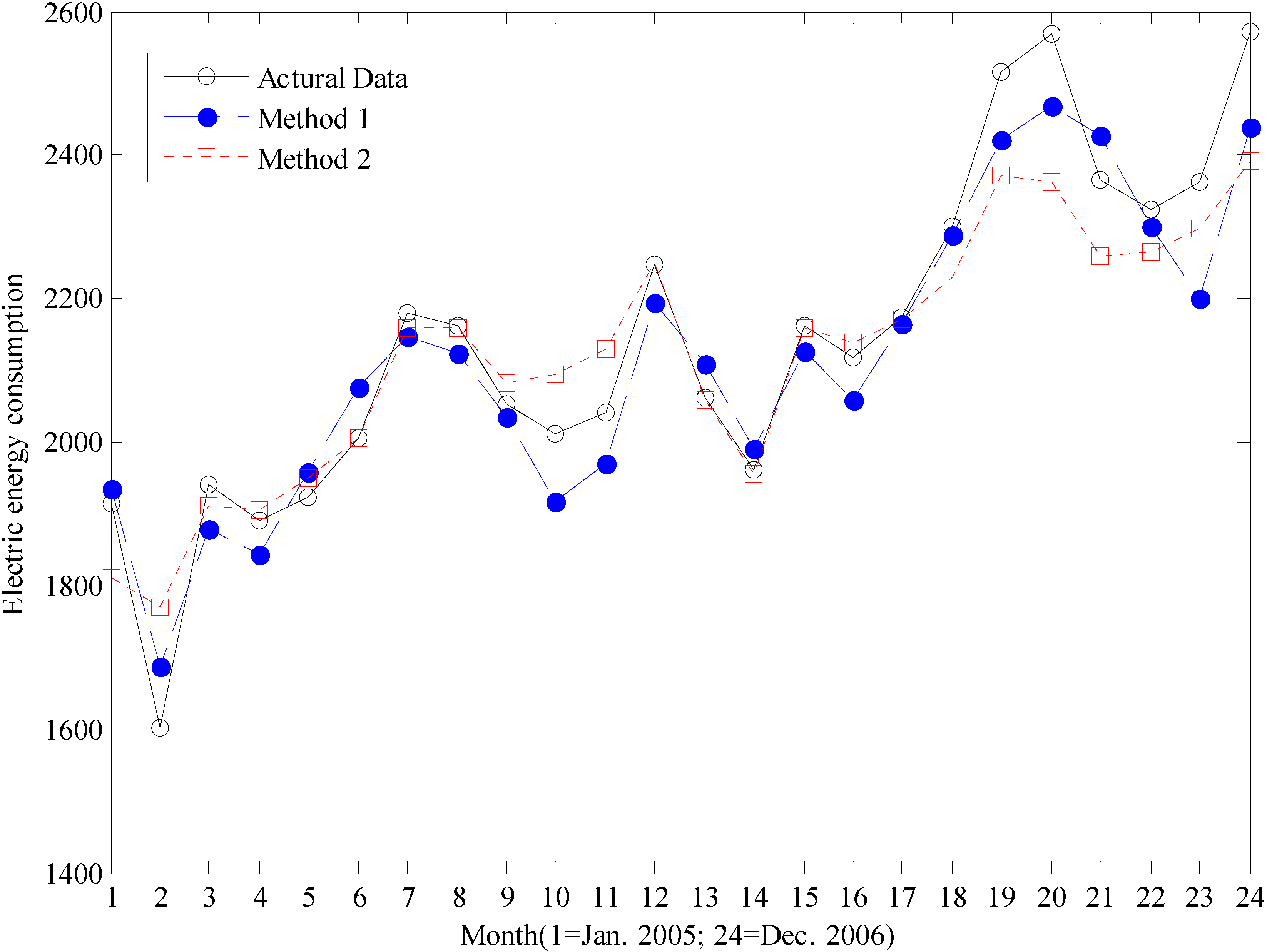
Compared with the traditional monthly electric energy consumption forecasting method proposed by González–Romera et al. [21] (hereinafter referred to as Method 2), two primary innovations are notable in Method 1. They are the applications of DWT and GM. To verify the contribution of each innovation, two transitional methods were designed. The NN used in the traditional method was replaced with GM (hereinafter Method 3), and the moving average algorithm in the traditional method was replaced with DWT (hereinafter Method 4). Furthermore, the traditional method was also used as a basis for modeling the monthly electric energy consumption data for China. The forecasting results of Methods 2, 3, and 4 are also listed in Table 1. To demonstrate the forecasting results intuitively, the curves of actual data and the forecasting results of Methods 1 and 2 were drawn (see Figure 5).

Figure 5. Curves of actual data based on the forecasting results of Methods 1 and 2.

Figure 5. Curves of actual data based on the forecasting results of Methods 1 and 2.

The maximal absolute percentage error (MaxAPE), mean absolute percentage error (MAPE), median absolute percentage error (MdAPE), and geometric mean relative absolute error (GMARE) were used as indicators of forecasting precision:

$$\text{MaxAPE}=\underset{i}{\text{max}}\left(\left|\frac{x(i)-\widehat{x}(i)}{x(i)}\right|\right)\times 100, i=1,2,\mathrm{...},N$$

(13)

where x(i) is the electric energy consumption value in the ith month; $\widehat{x}(i)$ represents its forecasting result; and N is the number of data used for the MAPE calculation:

$$\text{MAPE}=\frac{1}{N}{\displaystyle \sum _{i=1}^N\left|\frac{x(i)-\widehat{x}(i)}{x(i)}\right|}\times 100$$

(14)

$$\text{MdAPE}=\underset{i}{\text{median}}\left(\left|\frac{x(i)-\widehat{x}(i)}{x(i)}\right|\right)\times 100, i=1,2,\mathrm{...},N$$

(15)

$$\text{GMARE}={\left[{\displaystyle \prod _{i=1}^N\left|\frac{x(i)-\widehat{x}(i)}{x(i)-{\widehat{x}}^{*}(i)}\right|}\right]}^{\frac{1}{N}}$$

(16)

where ${\widehat{x}}^{*}(i)$ is the forecasting result obtained from the benchmark method. The results of the above indicators are listed in Table 2.

Table 2. Results of forecasting precision indicators.

	Method 1	Method 2	Method 3	Method 4
MaxAPE	6.94	10.6	8.79	7.16
MAPE	2.67	2.76	2.76	2.73
MdAPE	2.42	1.44	2.01	2.44
GMARE	0.61	0.33	0.51	0.63

Table 2. Results of forecasting precision indicators.

	Method 1	Method 2	Method 3	Method 4
MaxAPE	6.94	10.6	8.79	7.16
MAPE	2.67	2.76	2.76	2.73
MdAPE	2.42	1.44	2.01	2.44
GMARE	0.61	0.33	0.51	0.63

Compared with the Method 2, the application of GM (Method 3) has similar forecasting precision (MAPE) with less forecasting risk (MaxAPE). This finding proves that Method 3 performs better than Method 2 in terms of mitigating the stochastic effect on the primary trend. The application of DWT (Method 4) improves both the forecasting precision and forecasting risk. This result proves the positive effects of DWT in simplifying the periodic waves and eliminating the stochastic effects. When Method 1 is used, the MAPE and maximum error are both further reduced. This finding proves that Method 1 performs better than Method 2 in terms of both forecasting precision and risk. The variance of absolute percentage error of Methods 1, 2, 3, and 4 were 2.72, 8.18, 5.65, and 2.82. The biggest variance value of Methods 2 was the root cause of smallest GMARE and made it possible to obtain the smallest MAPE. Furthermore, the wave amplitude of the actual data increases with time, as shown in Figure 3, Figure 4 and Figure 5. The performance of Method 1 is acceptable for simulating this feature. The wave amplitude of Method 2 tends to be invariable, thereby resulting in poor forecasting performance.

4. Conclusions

The difficulties in forecasting monthly electric energy consumption are attributable to the excessive information in the values relative to the limited number of samples. In the current paper, the DWT is adopted to extract the features of monthly data into several relatively simple series. After the elimination of the stochastic series, the rising trend and other periodic waves are retained. To mitigate the stochastic effect on the primary trend, the GM is selected to model the rising trend of the retained components. Considering the increasing amplitude of retained periodic waves, the RBF NN is selected for use in simulation. Summing up the forecasting values of the GM and RBF NNs will yield the forecasting result of monthly electric energy consumption. The values of for 24 consecutive months of electric energy consumption in China are forecasted to test the effect of the proposed method. Compared with the traditional method, the following conclusions are confirmed: first, the primary contribution of GM is the reduction of the maximum forecasting error; second, the application of DWT in forecasting may result in a simultaneous reduction of the MAPE and maximum error, and third, when GM and DWT are used simultaneously, the MAPE and maximum error are both further reduced. In summary, the method proposed in the present study performs better in terms of forecasting precision and expected risk.

References

- Papalexopoulos, A.D.; Hesterberg, T.C. A regression-based approach to short-term load forecasting. IEEE Trans. Power Syst. 1990, 5, 1535–1550. [Google Scholar] [CrossRef]
- Rahman, S.; Hazim, O. A generalized knowledge-based short-term loadforecasting technique. IEEE Trans. Power Syst. 1993, 8, 508–514. [Google Scholar] [CrossRef]
- Abdel-Aal, R.E.; Al-Garni, A.Z. Forecasting monthly electric energy consumption in Eastern Saudi Arabia using univariate time-series analysis. Energy 1997, 22, 1059–1069. [Google Scholar] [CrossRef]
- Saab, S.; Badr, E.; Nasr, G. Univariate modeling and forecasting of energy consumption: The case of electricity in Lebanon. Energy 2001, 26, 1–14. [Google Scholar] [CrossRef]
- Hong, W.C.; Dong, Y.; Lai, C.-Y.; Chen, L.-Y.; Wei, S-Y. SVR with Hybrid Chaotic Immune Algorithm for Seasonal Load Demand Forecasting. Energies 2011, 4, 960–977. [Google Scholar] [CrossRef]
- Reis, A.J.R.; Silva, A.P.A.D. Feature extraction via multiresolution analysis for short-term load forecasting. IEEE Trans. Power Syst. 2005, 20, 189–198. [Google Scholar] [CrossRef]
- Kandil, N.; Wamkeue, R.; Saad, M.; Georges, S. An efficient approach for short term load forecasting using artificial neural networks. Int. J. Electr. Power Energy Syst. 2006, 28, 525–530. [Google Scholar] [CrossRef]
- Lauret, P.; Fock, E.; Randrianarivony, R.N.; Manicom-Ramsamy, J.-F. Bayesian neural network approach to short time load forecasting. Energy Convers. Manag. 2008, 49, 1156–1166. [Google Scholar] [CrossRef]
- Xiao, Z.; Ye, S.-J.; Zhong, B.; Sun, C.-X. BP neural network with rough set for short term load forecasting. Expert Syst. Appl. 2009, 36, 273–279. [Google Scholar] [CrossRef]
- Amjady, N.; Keynia, F. A new neural network approach to short term load forecasting of electrical power systems. Energies 2011, 4, 488–503. [Google Scholar] [CrossRef]
- Amjady, N.; Keynia, F. Day-ahead price forecasting of electricity markets by mutual information technique and cascaded neuro-evolutionary algorithm. IEEE Trans. Power Syst. 2009, 24, 306–318. [Google Scholar] [CrossRef]
- Amjady, N.; Keynia, F. A new prediction strategy for price spike forecasting of day-ahead electricity markets. Appl. Soft Comput. 2011, 11, 4246–4256. [Google Scholar] [CrossRef]
- Hagan, M.T.; Demuth, H.B.; Beale, M.H. Neural Network Design; PWS Publishing Company: Boston, MA, USA, 1996. [Google Scholar]
- Haykin, S. Neural Networks: A Comprehensive Foundation; Pearson Education Inc.: Upper Saddle River, NJ, USA, 2009. [Google Scholar]
- Parkpoom, S.J.; Harrison, G.P. Analyzing the impact of climate change on future electricity demand in Thailand. IEEE Trans. Power Syst. 2008, 23, 1441–1448. [Google Scholar] [CrossRef]
- Abdel-Aal, R.E. Univariate modeling and forecasting of monthly energy demand time series using abductive and neural networks. Comput. Ind. Eng. 2008, 54, 903–917. [Google Scholar] [CrossRef]
- Chang, P.-C.; Fan, C.-Y.; Lin, J.-J. Monthly electricity demand forecasting based on a weighted evolving fuzzy neural network approach. Int. J. Electr. Power Energy Syst. 2011, 33, 17–27. [Google Scholar] [CrossRef]
- Zhao, S.; Wei, G.W. Jump process for the trend estimation of time series. Comput. Stat. Data Anal. 2003, 42, 219–241. [Google Scholar] [CrossRef]
- González-Romera, E.; Jaramillo-Morán, M.A.; Carmona-Fernández, D. Monthly electric energy demand forecasting based on trend extraction. IEEE Trans. Power Syst. 2006, 21, 1946–1953. [Google Scholar] [CrossRef]
- González-Romera, E.; Jaramillo-Morán, M.A.; Carmona-Fernández, D. Forecasting of the electric energy demand trend and monthly fluctuation with neural networks. Comput. Ind. Eng. 2007, 52, 336–343. [Google Scholar] [CrossRef]
- González-Romera, E.; Jaramillo-Morán, M.A.; Carmona-Fernández, D. Monthly electric energy demand forecasting with neural networks and Fourier series. Energy Convers. Manag. 2008, 49, 3135–3142. [Google Scholar] [CrossRef]
- Saravanan, N.; Ramachandran, K.I. Incipient gear box fault diagnosis using discrete wavelet transform (DWT) for feature extraction and classification using artificial neural network (ANN). Expert Syst. Appl. 2010, 37, 4168–4181. [Google Scholar] [CrossRef]
- Deng, J.-L. Control problems of grey systems. Syst. Control Lett. 1982, 1, 288–294. [Google Scholar] [CrossRef]
- Deng, J.-L. Grey Forecasting and Decision; Huazhong University of Science & Technology Press Co.: Hangzhou, China, 2002. [Google Scholar]
- China Center for Economic Research (CCER). Chinese Economic and Financial Database 2011. Available online: http://www.ccerdata.com (accessed on 30 April 2011).
© 2011 by the authors; licensee MDPI, Basel, Switzerland. This article is an open access article distributed under the terms and conditions of the Creative Commons Attribution license (http://creativecommons.org/licenses/by/3.0/).
Share and Cite
MDPI and ACS Style
Meng, M.; Niu, D.; Sun, W. Forecasting Monthly Electric Energy Consumption Using Feature Extraction. Energies 2011, 4, 1495-1507. https://doi.org/10.3390/en4101495
AMA Style
Meng M, Niu D, Sun W. Forecasting Monthly Electric Energy Consumption Using Feature Extraction. Energies. 2011; 4(10):1495-1507. https://doi.org/10.3390/en4101495
Chicago/Turabian StyleMeng, Ming, Dongxiao Niu, and Wei Sun. 2011. "Forecasting Monthly Electric Energy Consumption Using Feature Extraction" Energies 4, no. 10: 1495-1507. https://doi.org/10.3390/en4101495