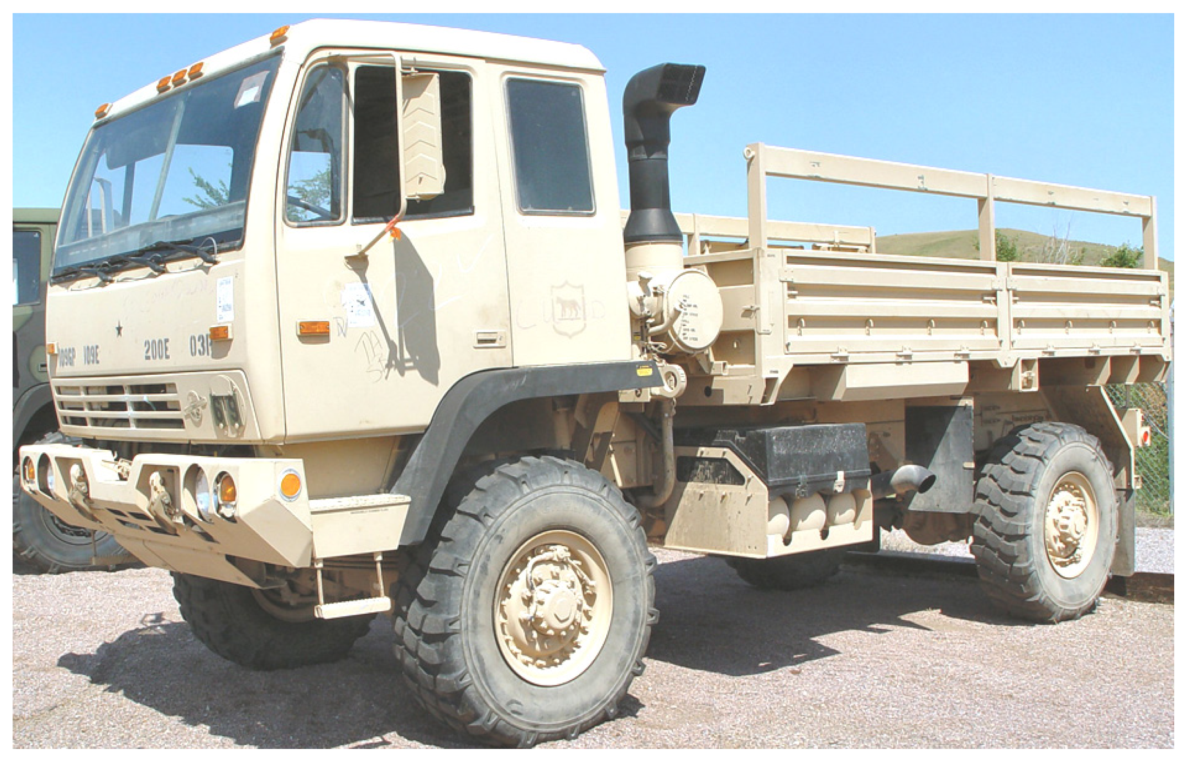
Experiment and Simulation of Medium-Duty Tactical Truck for Fuel Economy Improvement

Abstract
:1. Introduction

| Vehicle Component | Specification |
|---|---|
| Wheel base | 3900 mm (153.5") |
| Vehicle curb weight (no kits, crew, fuel) | 7809 kg (17,216 lb) |
| Payload | 2268 kg (5000 lb) plus kits |
| Towed load | 5443 kg (12,000 lb) |
| Maximum speed(governed, at gross weight) | 94 kph (km/h) or 58 mile/h (mph) |
| Range—58 gal (219 L) nominal | 645 km (400 mile) |
| Maximum grade/side slope | 60%/30% |
| Engine: | Caterpillar C7 ATAAC (air-to-air after cooler) HD diesel, in-line 6-cylinder, 4-stroke-cycle |
| Displacement | 7.2 L (441 cubic inch) |
| Aspiration | Turbocharged—air-to-air aftercooler, EPA 07 certified |
| Rating | 205 kW (275 hp) @ 2600 rpm |
| Torque | 1166 Nm (860 lb-ft) @ 1440 rpm |
| Fuel system | Electronic injection |
| Fuel types | Diesel, DF-2, JP-4, JP-8 |
| Transmission: | Allison 3700SP, 7-speed automatic, electronically controlled, full-time all-wheel drive |
| Front wheels | 30% torque |
| Rear wheels | 70% torque |
| Axles: Front/rear axles | ArvinMeritor |
| Overall axle gear ratio | 7.8:1 |
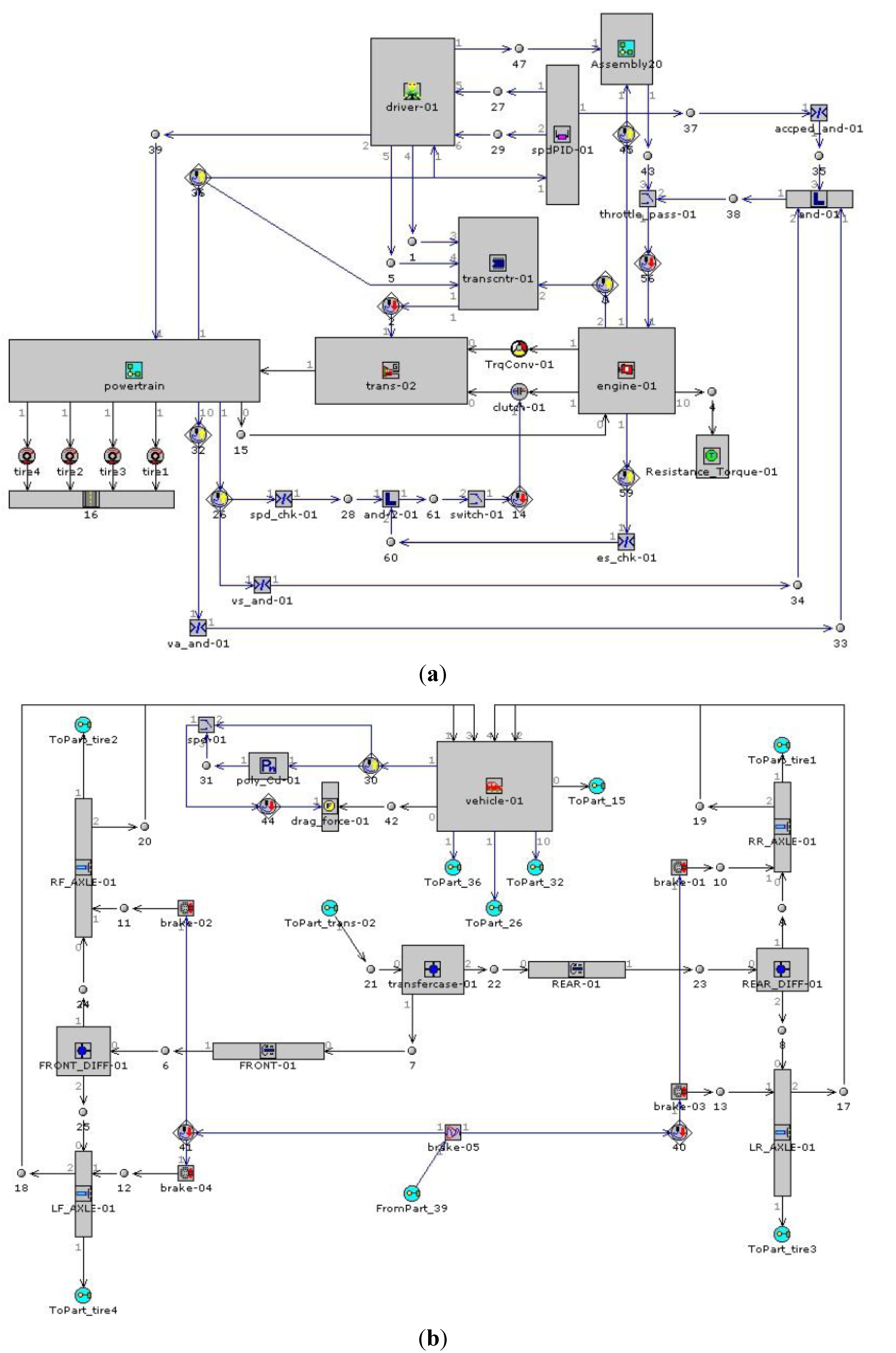
2. Analytical Vehicle Model and Experimental Test of Baseline Vehicle
2.1. Baseline Vehicle Model
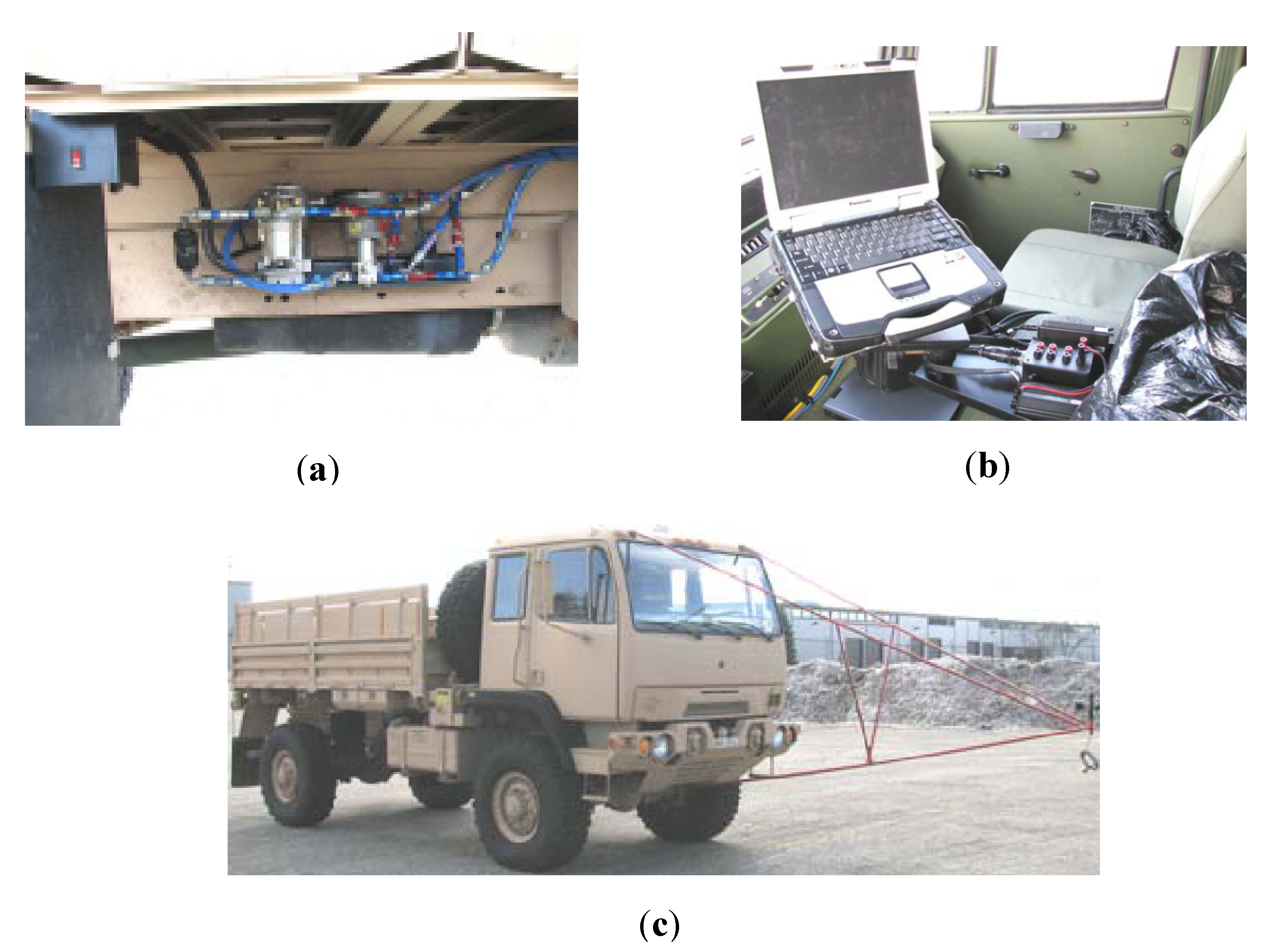
2.2. Baseline Vehicle Experimental Testing

- •
- The decrease in the aerodynamic drag due to lift forces is very small and disregarded.
- •
- The tire slip angle due to aerodynamic side forces and yawing moments are negligible and do not influence the tire rolling resistance.
- •
- The variation of the rolling resistance with vehicle speed can be adequately modeled with a second degree function of vehicle speed.
- •
- The variation of the aerodynamic drag coefficient over the speed range of the test is negligible.
- •
- The variation of the aerodynamic drag coefficient with yaw angle can be adequately modeled with a fourth degree function of yaw angle.
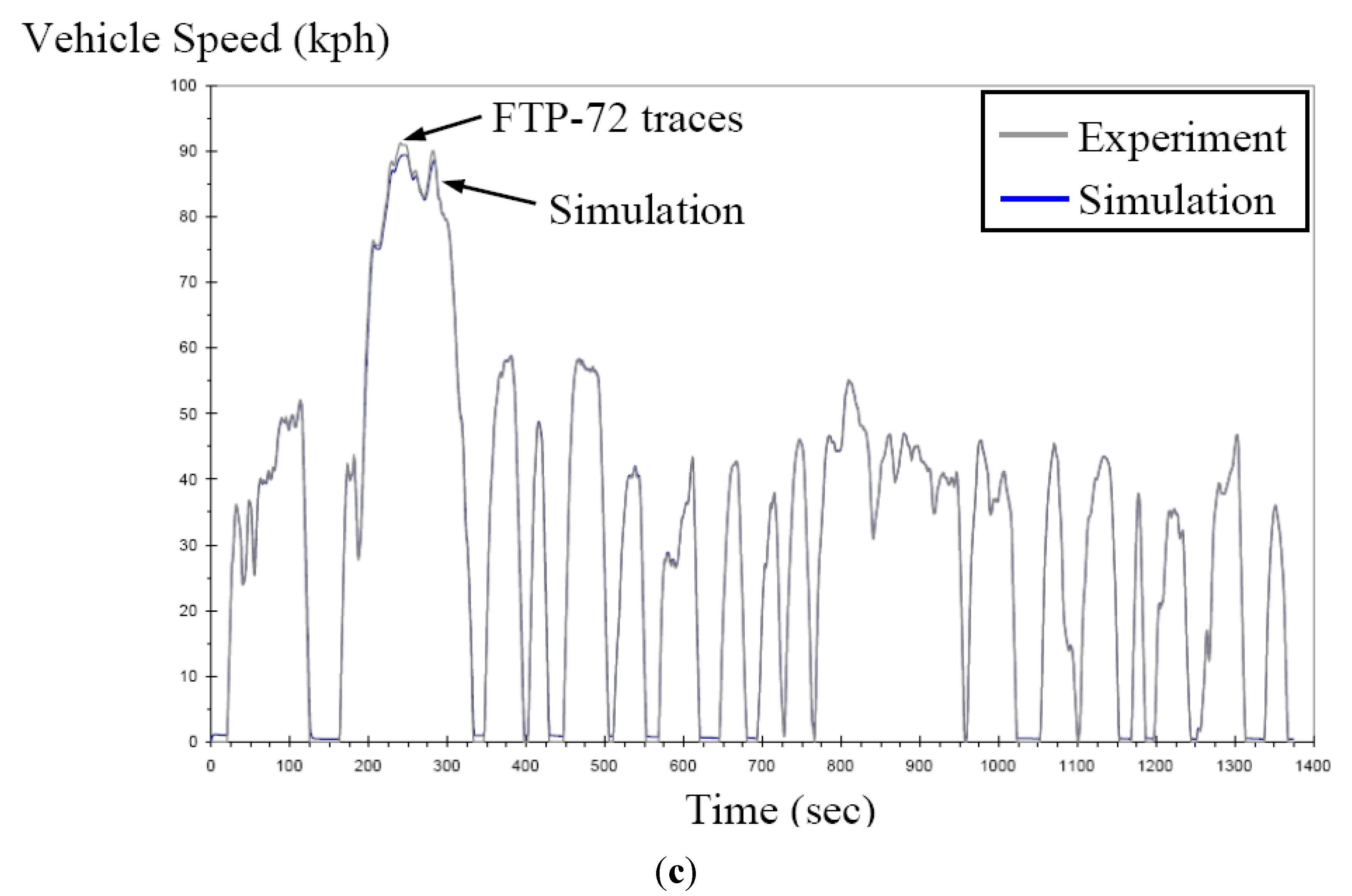
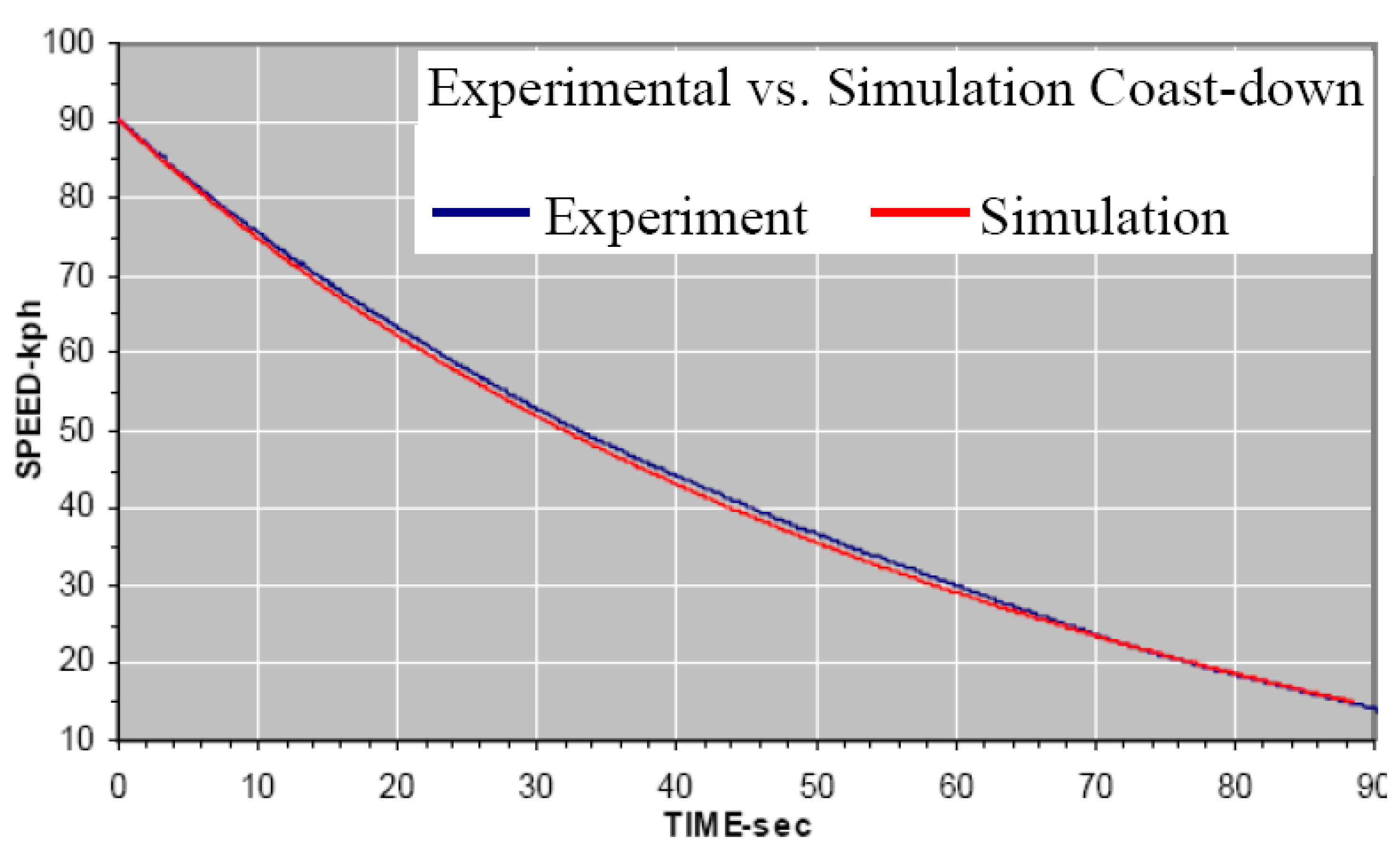
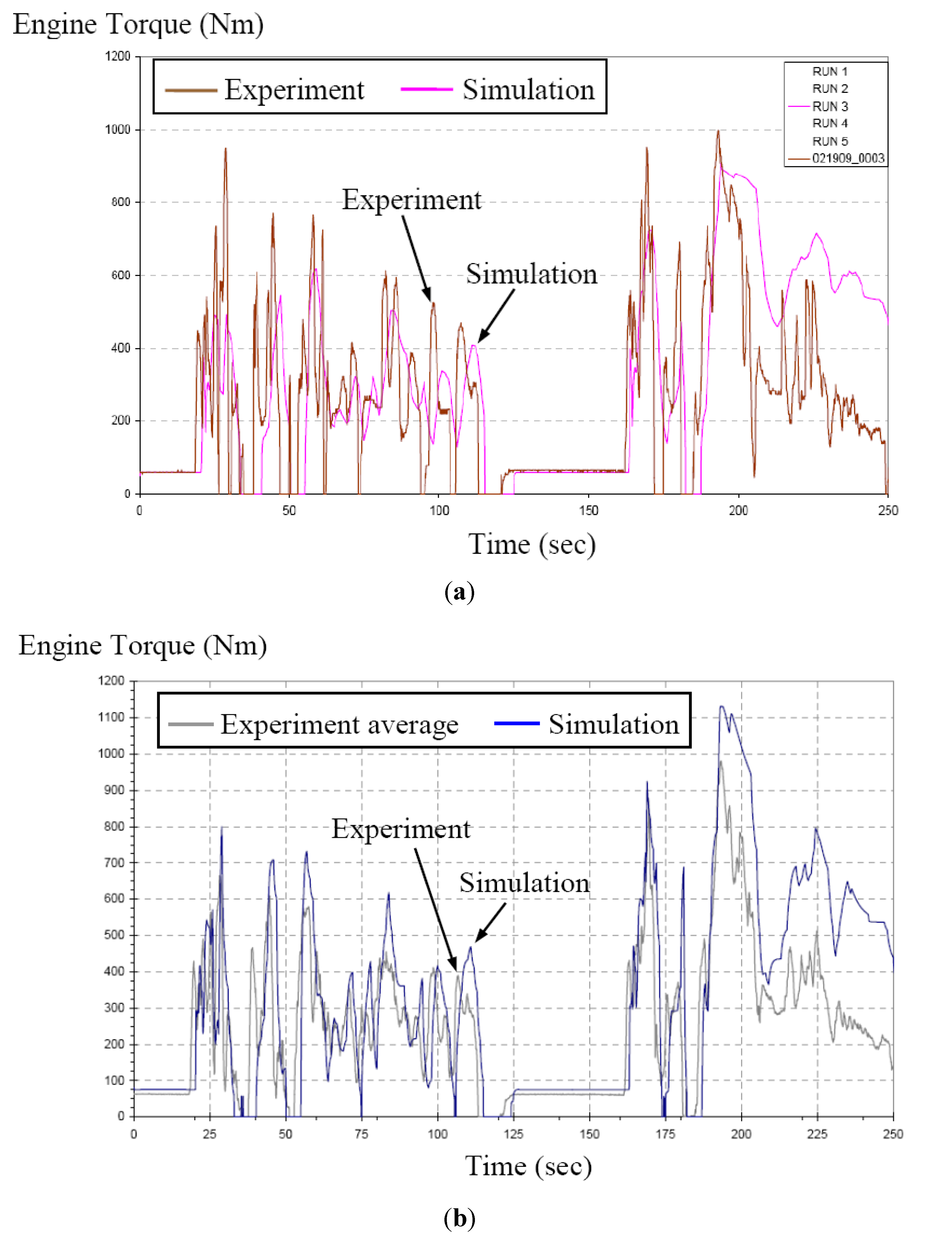
2.3. Correlation between Simulation and Experimental Baseline Vehicle
| Run No. | Test Time (sec) | Simulation Time (sec) | ΔT (Simulation Time − Test Time) | % Error (ΔT/Test Time) |
|---|---|---|---|---|
| 1 | 75.8 | 76.672 | 0.872 | 1.1% |
| 2 | 84.3 | 79,104 | −5.196 | −6.6% |
| 3 | 74.1 | 72.704 | −1.396 | −1.9% |
| 4 | 78.8 | 77.056 | −1.744 | −2.3% |
| 5 | 76.6 | 76.928 | 0.328 | 0.4% |
| 6 | 77.1 | 75.648 | −1.452 | −1.9% |
| 7 | 73.0 | 75.264 | 2.264 | 3.0% |
| 8 | 75.8 | 73.856 | −1.944 | −2.6% |
| 9 | 72.0 | 67.328 | −4.672 | −6.9% |
| Gear No. | Gear Ratio | Gear Ratio Step Fraction | Inertia (kg m2) | Efficiency |
|---|---|---|---|---|
| 1 | 6.93 | 1.658 | 0.16 | 0.954 |
| 2 | 4.18 | 1.866 | 0.17 | 0.961 |
| 3 | 2.24 | 1.325 | 0.20 | 0.971 |
| 4 | 1.69 | 1.408 | 0.23 | 0.975 |
| 5 | 1.20 | 1.333 | 0.34 | 0.980 |
| 6 | 0.90 | 1.154 | 0.46 | 0.980 |
| 7 | 0.78 | 0.66 | 0.980 |
| Vehicle Speed Based Shift Schedule | ||||||
|---|---|---|---|---|---|---|
| Up-shift event | 1−2 | 2−3 | 3−4 | 4−5 | 5−6 | 6−7 |
| Vehicle speed (kph) | 11.05 | 28.23 | 22.46 | 33.67 | 53.68 | |
| Down-shift event | 2−1 | 3−2 | 4−3 | 5−4 | 6−5 | 7−6 |
| Vehicle speed (kph) | 8.72 | 16.95 | 24.05 | 31.99 | 47.30 | |

3. Modeling and Simulation of Vehicle with AMT
| Gear No. | Gear Ratio | Gear Ratio Step Fraction | Inertia (kg m2) | Efficiency |
|---|---|---|---|---|
| Lo-Lo | 14.56 | 1.546 | 0.110 | 0.94 |
| Low | 9.420 | 1.510 | 0.150 | 0.95 |
| 1 | 6.240 | 1.348 | 0.160 | 0.96 |
| 2 | 4.630 | 1.362 | 0.165 | 0.96 |
| 3 | 3.400 | 1.344 | 0.180 | 0.96 |
| 4 | 2.530 | 1.383 | 0.190 | 0.96 |
| 5 | 1.830 | 1.346 | 0.220 | 0.98 |
| 6 | 1.360 | 1.360 | 0.290 | 0.98 |
| 7 | 1.000 | 1.351 | 0.400 | 0.99 |
| 8 | 0.740 | 0.700 | 0.98 |
| Vehicle Speed Based Shift Schedule—Optimization | |||||||||
|---|---|---|---|---|---|---|---|---|---|
| Up-shift event | 1–2 | 2–3 | 3–4 | 4–5 | 5–6 | 6–7 | 7–8 | 8–9 | 9–10 |
| Vehicle speed (kph) | 4.69 | 7.44 | 11.43 | 15.07 | 21.69 | 29.15 | 41.18 | 55.35 | 63.99 |
| Down-shift event | 2–1 | 3–2 | 4–3 | 5–4 | 6–5 | 7–6 | 8–7 | 9–8 | 10–9 |
| Vehicle speed (kph) | 4.26 | 6.85 | 9.23 | 12.57 | 16.72 | 25.68 | 39.84 | 41.15 | 58.68 |
| Gear No. | Gear Ratio | Gear Ratio Step Fraction | Inertia (kg m2) | Efficiency |
|---|---|---|---|---|
| 1 | 12.326 | 1.285 | 0.118 | 0.95 |
| 2 | 9.590 | 1.290 | 0.186 | 0.95 |
| 3 | 7.435 | 1.285 | 0.123 | 0.95 |
| 4 | 5.784 | 1.267 | 0.195 | 0.96 |
| 5 | 4.565 | 1.296 | 0.137 | 0.96 |
| 6 | 3.522 | 1.304 | 0.218 | 0.96 |
| 7 | 2.700 | 1.285 | 0.155 | 0.97 |
| 8 | 2.101 | 1.290 | 0.247 | 0.97 |
| 9 | 1.629 | 1.286 | 0.225 | 0.98 |
| 10 | 1.267 | 1.267 | 0.362 | 0.98 |
| 11 | 1.000 | 1.285 | 0.406 | 0.99 |
| 12 | 0.778 | 0.662 | 0.98 |
| Vehicle Speed Based Shift Schedule—Optimization | |||||||||||
|---|---|---|---|---|---|---|---|---|---|---|---|
| Up-shift event | 1–2 | 2–3 | 3–4 | 4–5 | 5–6 | 6–7 | 7–8 | 8–9 | 9–10 | 10–11 | 11–12 |
| Vehicle speed (kph) | 5.51 | 7.05 | 9.00 | 11.65 | 14.79 | 19.87 | 26.67 | 34.45 | 43.83 | 55.65 | 63.77 |
| Down-shift event | 2–1 | 3–2 | 4–3 | 5–4 | 6–5 | 7–6 | 8–7 | 9–8 | 10–9 | 11–10 | 12–11 |
| Vehicle speed (kph) | 4.23 | 5.75 | 7.39 | 9.37 | 12.29 | 15.83 | 24.48 | 31.49 | 43.13 | 50.80 | 63.14 |
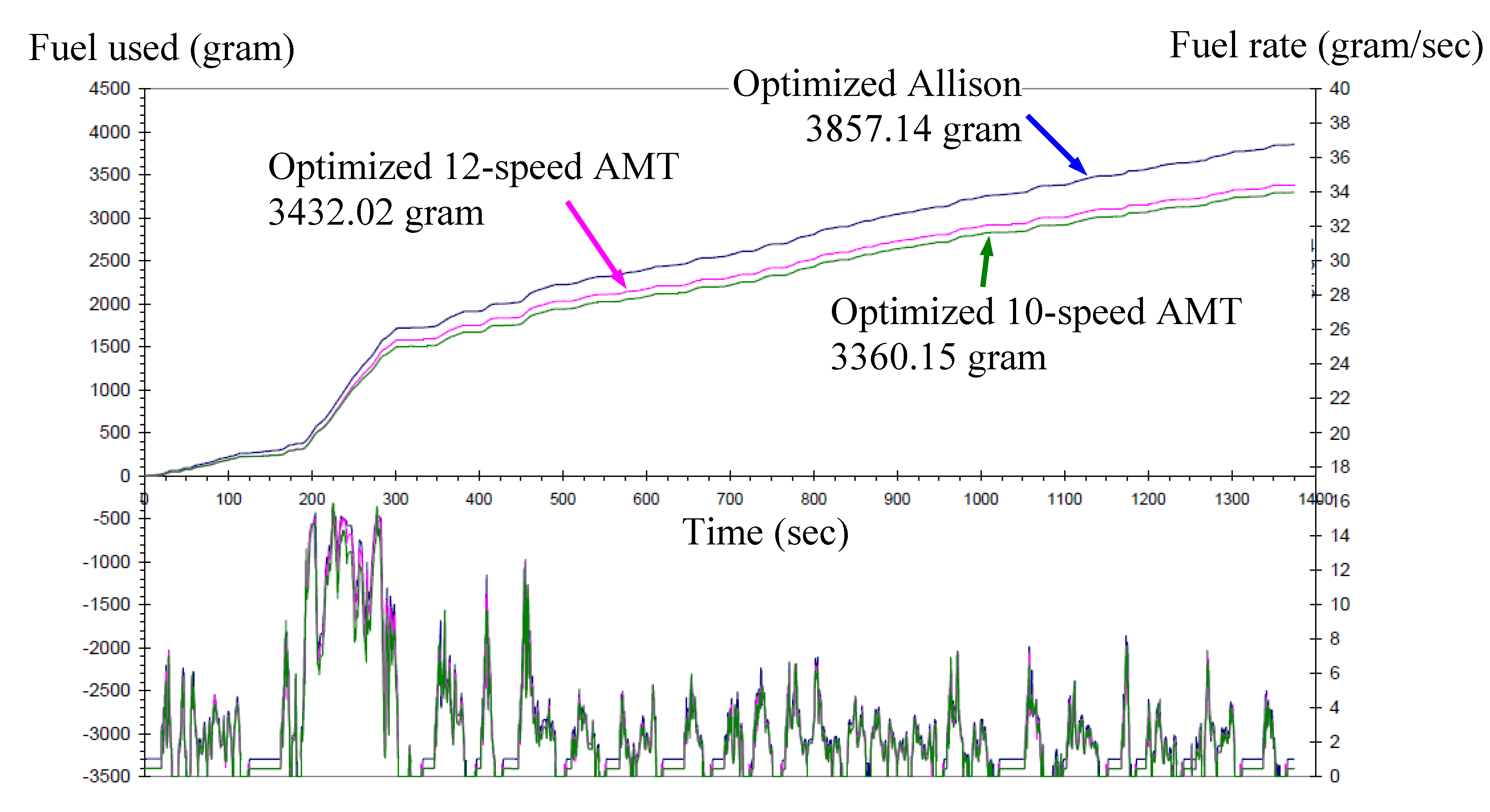
4. Comparisons of Fuel Economy Simulation Results

5. Conclusions
| Total Fuel Used (gram) | Fuel Economy liter/km (mi/gal) | % Improvement | |
|---|---|---|---|
| Experimental average | 3807.39 | 0.375 (6.27) | |
| Allison baseline | 3921.26 | 0.386 (6.09) | |
| Allison optimized shift schedule | 3857.14 | 0.380 (6.19) | 1.64 |
| 10-speed AMT | 3360.15 | 0.331 (7.09) | 14.5 |
| 12-speed AMT | 3432.02 | 0.338 (6.95) | 12.2 |
| Allison baseline | 3921.26 | 0.386 (6.09) | |
| Engine idle stop/start | 3788.47 | 0.373 (6.31) | 3.4 |
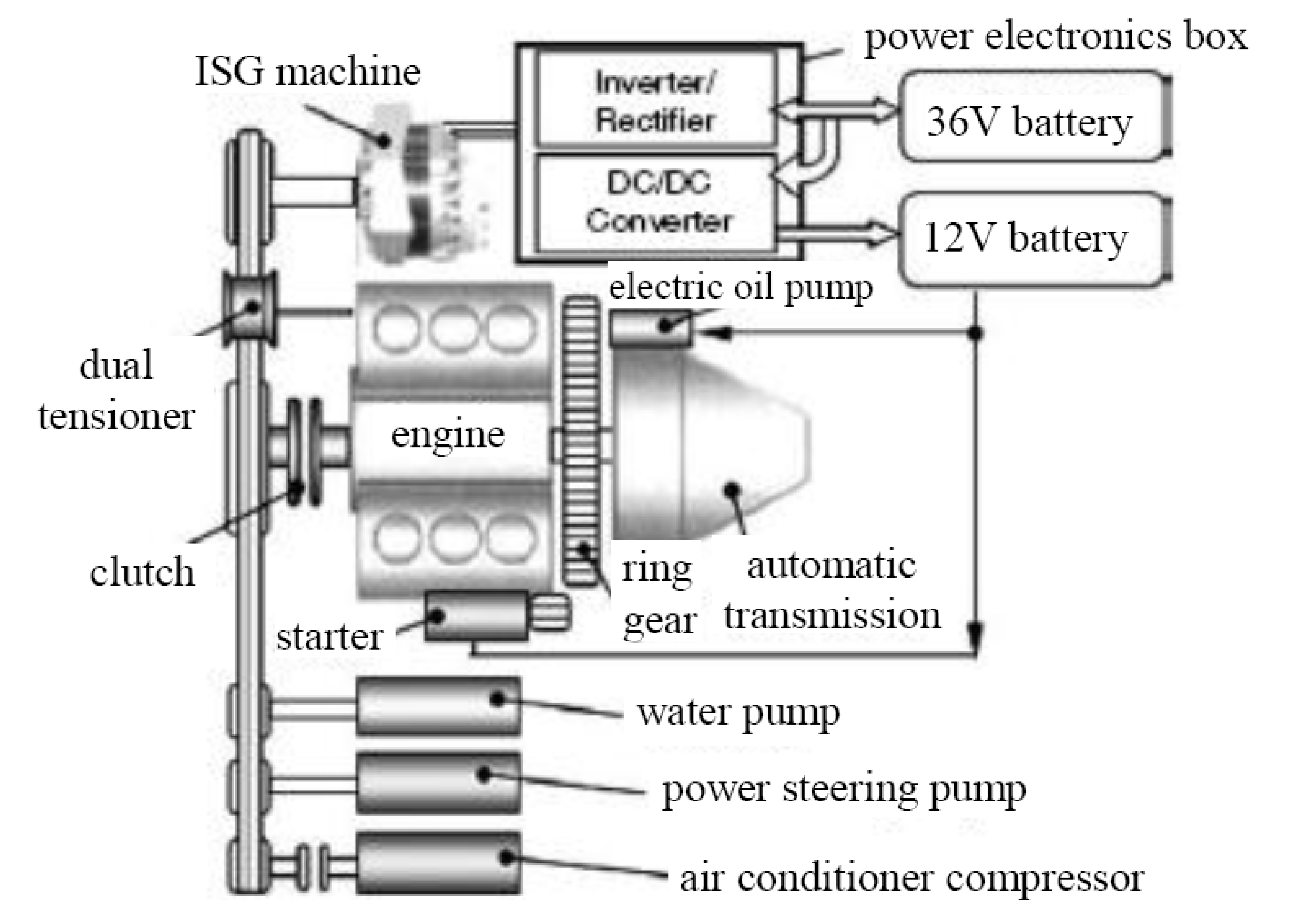
| B-ISG mild hybridization | 3521.86 | 0.347 (6.72) | 10.2 |
Acknowledgements
References
- U.S. Department of Defense. More Capable War Fighting through Reduced Fuel Burden; Technical Report for Office of the Under Secretary of Defense for Acquisition; Technology and Logistics: Washington, DC, USA, May 2001. [Google Scholar]
- Muradian, V. Interview with Terry Pudas, Acting Deputy Assistant Secretary of Defense for Forces, Transformation and Resources. Defense News 2007, 22. [Google Scholar]
- Karbuz, S. US military energy consumption—facts and figures. Available online: http://www.energybulletin.net/node/29925/ (accessed on 18 October 2010).
- BAE Systems. Available online: http://www.baesystems.com/Newsroom/ (accessed on 26 January 2011).
- FMTV A1R M1078A1 data sheet, BAE Systems. Available online: http://www.baesystems.com/BAEProd/groups/public/documents/bae_publication/bae_pdf_mps_fmtv_m1078a1.pdf/ (accessed on 30 October 2010).
- Kuroiwa, H.; Ozaki, N.; Okada, T.; Yamasaki, M. Next-generation fuel-efficient automated manual transmission. SAE Paper 2004, 53, 205–209. [Google Scholar]
- Heath, R.P.; Child, A.J. A seamless automated manual transmission (AMT) with no torque interrupt. SAE Paper 2007. [Google Scholar] [CrossRef]
- Yamamoto, K.; Aoki, T. Analysis of the influence on fuel economy by transmission type and the estimation of fuel economy. Jpn. Sci. Technol. Agency 2000, 12, 63–72. [Google Scholar]
- Song, X.Y.; Sun, Z.X.; Yang, X.J.; Zhu, G.M. Modelling, control, and hardware-in-the-loop simulation of an automated manual transmission. Proc. Inst. Mech. Eng. D J. Automobile Eng. 2010, 224, 143–160. [Google Scholar] [CrossRef]
- Zhang, Y.; Chen, X.; Zhang, X.; Jiang, H.; Tobler, W. Dynamic modeling and simulation of a dual-clutch automated lay-shaft transmission. ASME J. Mech. Des. 2005, 127, 302–307. [Google Scholar] [CrossRef]
- Kusumi, H.; Yagi, K.; Ny, Y.; Abo, S.; Furuta, S.; Morikawa, M. 42V power control system for Mild Hybrid Vehicle (MHV). SAE Paper 2002. [Google Scholar] [CrossRef]
- Tamai, G.; Jeffers, M.; Lo, C.; Thurston, C.; Tarnowsky, S.; Poulos, S. Development of the hybrid system for the Saturn VUE hybrid. SAE Paper 2006. [Google Scholar] [CrossRef]
- Canova, M.; Sevel, K.; Guezennec, Y.; Yukovich, S. Control of the start/stop of a diesel engine in a parallel HEV with a belted starter/alternator. SAE Paper 2007. [Google Scholar] [CrossRef]
- Evans, D.; Polom, M.; Poulos, S.; VanMaanen, K.; Zarger, T. Powertrain architecture and controls integration for GM’s hybrid full-size pickup truck. SAE Paper 2003. [Google Scholar] [CrossRef]
- Chen, X.; Shen, S. Comparison of two permanent-magnet machines for a mild hybrid electric vehicle application. SAE Paper 2008. [Google Scholar] [CrossRef]
- Hanada, K.; Kaizuka, M.; Ishikawa, S.; Imai, T.; Matsuoka, H.; Adach, H. Development of a hybrid system for the V6 midsize sedan. SAE Paper 2005. [Google Scholar] [CrossRef]
- Kabasawa, A.; Takahashi, K. Development of the IMA motor for the V6 hybrid midsize sedan. SAE paper 2005. [Google Scholar] [CrossRef]
- van Benschoten, M.; Nelson, E. FMTV transmission fuel economy study: Evaluation of AMT performance using experimental and analytical methods. In Proceedings of the 2009 Ground Vehicle Systems Engineering and Technology Symposium (GVSETS), Detroit, MI, USA, 28 May 2009.
- GT-Drive, Gamma Technologies, Inc. Virtual Engine/Powertrain/Vehicle Simulation. Available online: http://www.gtisoft.com/GT-SUITE_Product.html/ (accessed on 15 October 2010).
- Hausberger, S.; Rexeis, M. Emission behaviour of modern heavy duty vehicles in real world driving. Int. J. Environ. Pollut. 2004, 22, 275–286. [Google Scholar] [CrossRef]
- Ward, M.; Brace, C.; Hale, T.; Ceen, R. Investigation of sweep mapping approach on engine testbed. SAE Paper 2002. [Google Scholar] [CrossRef]
- Pacejka, H.B. Tyre and Vehicle Dynamics; Butterworth-Heineman: Oxford, UK, 2002. [Google Scholar]
- Hucho, W.H. Aerodynamics of Road Vehicles; SAE International: Troy, MI, USA, 1998. [Google Scholar]
- U.S. Environmental Protection Agency. Testing and Measuring Emissions. Available online: http://www.epa.gov/nvfel/testing/ dynamometer.html/ (accessed on 12 October 2010).
- Ivarsson, M.; Slund, J.; Nielsen, L. Impacts of AMT gear-shifting on fuel optimal look ahead control. SAE Paper 2010. [Google Scholar] [CrossRef]
© 2011 by the authors; licensee MDPI, Basel, Switzerland. This article is an open access article distributed under the terms and conditions of the Creative Commons Attribution license (http://creativecommons.org/licenses/by/3.0/).
Share and Cite
Liao, Y.-J.G.; Quail, A.M., Jr. Experiment and Simulation of Medium-Duty Tactical Truck for Fuel Economy Improvement. Energies 2011, 4, 276-293. https://doi.org/10.3390/en4020276
Liao Y-JG, Quail AM Jr. Experiment and Simulation of Medium-Duty Tactical Truck for Fuel Economy Improvement. Energies. 2011; 4(2):276-293. https://doi.org/10.3390/en4020276
Chicago/Turabian StyleLiao, Yeau-Jian Gene, and Allen M. Quail, Jr. 2011. "Experiment and Simulation of Medium-Duty Tactical Truck for Fuel Economy Improvement" Energies 4, no. 2: 276-293. https://doi.org/10.3390/en4020276