Impact of Turbulence Intensity and Equivalence Ratio on the Burning Rate of Premixed Methane–Air Flames

Abstract

Direct Numerical Simulations (DNS) have been conducted to study the response of initially laminar spherical premixed methane–air flame kernels to successively higher turbulence intensities at five different equivalence ratios. The numerical experiments include a 16-species/25-step skeletal mechanism for methane oxidation and a multicomponent molecular transport model. Highly turbulent conditions (with integral Reynolds numbers up to $4513$) have been accessed. The effect of turbulence on the physical properties of the flame, in particular its consumption speed $S_c$, which is an interesting measure of the turbulent flame speed $S_T$ has been investigated. Local quenching events are increasingly observed for highly turbulent conditions, particularly for lean mixtures. The obtained results qualitatively confirm the expected trend regarding correlations between $u^{\prime }/S_L$ and the consumption speed: $S_c$ first increases, roughly linearly, with $u^{\prime }/S_L$ (low turbulence zone), then levels off (bending zone) before decreasing again (quenching limit) for too intense turbulence. For a fixed value of $u^{\prime }/S_L$, $S_c/S_L$ varies with the mixture equivalence ratio, showing that additional parameters should probably enter phenomenological expressions relating these two quantities.

1. Introduction

Premixed turbulent flames remain a significant research challenge in the combustion community. Their propagation is of significant and practical importance in the design and optimization of efficient low emission burners. One essential property is their turbulent burning velocity $S_T$ [1,2]. Its influential role in turbulent premixed flame modeling has attracted a wealth of experimental and theoretical investigations in a variety of flow configurations [3]. Experimental setups to measure $S_T$ differ from one study to another, and many challenges remain—unsteadiness and inhomogeneity of the flow, influence of the ignition source on the flame propagation, difficulties in quantifying heat losses and length scales—leading to a large scattering in the dataset of the latter for a fixed root-mean-square (rms) velocity to laminar flame velocity ratio, $u^{\prime }/S_L$; an accurate measurement of $S_T$ is still difficult (see e.g., [3,4] and references therein).

Considering the correlation of the ratio of turbulent to laminar burning velocities $S_T/S_L$ and $u^{\prime }/S_L$ [5], old experimental data reveal a steady linear increase of $S_T/S_L$ with $u^{\prime }/S_L$ [6] for the higher range of turbulence Reynolds number Re${}_t=u^{\prime }{l}_t/\nu$, where $l_t$ is the integral length scale and ν is the kinematic viscosity. This is contrary to the seminal investigations in, for instance, [2,7] for a lower range of Re${}_t$. While most combustion vessel experiments witness a global gas phase extinction at too intense turbulence, this is still considered as an open issue for other configurations and measurement techniques [8,9,10].

Beyond theoretical considerations and complex experimental measurements, numerical simulation, in particular, Direct Numerical Simulation (DNS) is now a widely accepted technique for investigating turbulent combustion problems. DNS provides a unique insight into the physics of flame–turbulence interactions (see e.g., [11] and references therein). The advent of advanced computer technology and the development of efficient computational algorithms have now made it possible to employ DNS with realistic models. Numerical investigation of multi-component multi-dimensional reactive flows are possible in long but affordable computing times, without compromising accuracy. All parameters can be determined in such numerical experiments at the same time, offering a high level of flexibility for determining specific quantities in details under prescribed conditions. This makes DNS a convenient tool for the generation of correlations between $S_T/S_L$ and $u^{\prime }/S_L$ for various flow and burning conditions.

Due to its practical relevance, methane is one of the first fuels for which reduced kinetic models have been developed, since the chemical complexity associated with its direct simulation using full reaction schemes is still often prohibitive. Consequently, a large proportion of numerical studies of hydrocarbon flames is confined either to simple and/or two-dimensional flows with full chemical kinetic schemes (see [12] and references therein) or to complex and/or three-dimensional flows with simple/reduced schemes (see [13] and references therein). However, it is worth noting that significant advances have been made in recent years towards simulating systems burning practically relevant fuels together with detailed and accurate models for both the chemical and transport phenomena [14,15,16]. Thanks to the rapid growth of computational capabilities, adequate numerical predictions of the turbulent burning velocity have been provided [17,18] up to laboratory scale configurations [19,20] using high fidelity DNS. Such numerical studies have shown that turbulence enhances the flame speed with a rate faster than the growth in flame surface area, which is consistent with earlier studies conducted with simple models. A recent review is given by Driscoll [3].

In the present work, direct simulations are used to investigate systematically premixed methane–air mixtures under successively higher turbulence intensities using detailed physicochemical models, with the aim of supplying complementary data of turbulent consumption speed $S_c$ (which is an interesting measure of the turbulent burning velocity $S_T$) as a function of turbulence intensity $u^{\prime }/S_L$. It is then possible to determine in particular if and how the turbulent Reynolds number directly affects $S_c$ for a given turbulence intensity; and if the still controversial “bending zone” and “quenching limit” on the $S_c$ curves versus $u^{\prime }/S_L$ can be captured numerically. The setup and range of parameters to be explored mimic combustion vessel experiments (see e.g., [2,7] and references therein). The computational settings are similar to those used in [13] for a single-step reaction mechanism and unity Lewis number assumption. In the present study, both the three-dimensional and turbulent nature of the flame–kernel evolution together with a skeletal reaction scheme and multi-component transport models are considered.

In the next section (Section 2), details of the Direct Numerical Simulations and general computational procedure are given. Two major fine-grain parallelism issues—the initial fluctuating velocity generation and data input/output scenarios—for the employed DNS solver are discussed briefly. The problem configuration and initialization is next outlined in Section 3, directly followed by the numerical results for the various considered cases in Section 4, just before concluding in Section 5.

2. Direct Numerical Simulation

A DNS must provide as far as possible an exact solution for both fluid dynamics and flame structure. Even though this method requires prohibitive numerical costs for practical engineering configurations at large scales, it offers an excellent complement to experiments in order to assess the importance of various physical mechanisms, to obtain complementary information on flame structure, and therefore to improve turbulent combustion modeling [21].

In this study, the massively parallel DNS flame solver parcomb [22] is used. It solves the full compressible reactive Navier-Stokes system coupled with detailed physicochemical models [23,24]. The solved balance equations are, using classical notations [25] and ignoring all external forces:

$$\frac{\partial \rho }{\partial t}+\frac{\partial \left(\rho u_j\right)}{\partial x_j}=0$$

(1)

$$\frac{\partial \left(\rho u_i\right)}{\partial t}+\frac{\partial \left(\rho u_j{u}_i\right)}{\partial x_j}=-\frac{\partial p}{\partial x_i}+\frac{\partial {\tau }_{ij}}{\partial x_j};i=1,2,3$$

(2)

$$\frac{\partial \left(\rho Y_k\right)}{\partial t}+\frac{\partial \left[\rho (u_j+V_{kj})Y_k\right]}{\partial x_j}={\dot{\omega }}_k;k=1,N_s$$

(3)

$$\frac{\partial \left(\rho e_t\right)}{\partial t}+\frac{\partial \left[(\rho e_t+p)u_j\right]}{\partial x_j}=-\frac{\partial q_j}{\partial x_j}+\frac{\partial \left({\tau }_{ij}{u}_i\right)}{\partial x_i}$$

(4)

$$\frac{p}{\rho }=\frac{R}{\overline{W}}T$$

(5)

where ρ denotes mixture density, $u_j$ the components of the hydrodynamic velocity, p the pressure, $N_s$ the total number of species, $V_{kj}$ the component of the diffusion velocity of species k in the direction j, ${\dot{\omega }}_k$ the chemical production rate of species k, $q_j$ the $j^{th}$-component of the heat flux vector and ${\tau }_{ij}$ the stress tensor:

$${\tau }_{ij}=\eta \left[\frac{\partial u_i}{\partial x_j}+\frac{\partial u_j}{\partial x_i}\right]-\frac{2}{3}\eta \frac{\partial u_k}{\partial x_k}{\delta }_{ij}$$

(6)

where δ is the Kronecker symbol and η is the dynamic viscosity.

A spatial sixth-order central scheme and an explicit fourth-order Runge-Kutta time integrator are employed. In its recent version [26,27,28], the skew-symmetric formulation [29] has been implemented for the convective terms in order to reduce even further numerical dissipation and increase stability. The extended Navier-Stokes Characteristic Boundary Conditions (NSCBC) [30] are used, with non-reflecting boundaries and pressure relaxation applied along all open faces. The parallelization is in a 3D block structure using the MPI protocol for data exchange. The code offers, for instance on the IBM BlueGene/P $13.5\%$ of the peak performance on each node (139 TeraFlop/s for the full machine) and a near perfect parallel scaling for a real, three-dimensional run using up to $4096$ PowerPC 450 computing cores. Further details concerning code structure, optimization, application and recent upgrades can be found for instance in [27,31].

In order to access higher values of Re${}_t$ on fine-grain parallel systems, two turbulence generators based on digital filters [32] and random noise diffusion [33] have been hybridized, implemented and parallelized on massively parallel computers. With this simple and flexible approach, the restriction on problem size imposed by the previously implemented generator based on inverse FFT has been removed, paving the way for simulations of larger domains at considerably higher Re${}_t$ values. For the results presented later, the initial turbulent field has been systematically generated using this hybrid technique (see [27] for further details).

The second major issue that needed attention towards fine-grain parallelism is that of efficient, fully parallel data input/output (I/O). The traditional sequential I/O approaches have been replaced by a fully parallel I/O (via MPI-I/O), where multiple processes of the parallel program access data (for read/write) from a common, shared file. This provides both higher performance (speedup in time needed for writing/reading all files by a factor of at least 3) and single (restart/solution) data files.

3. Flame Configuration and Initialization

Initially perfectly spherical laminar premixed methane–air flames are considered in all computations, within a cubic computational domain of sides $L=4.0$ cm (Figure 1a) and a uniform grid spacing of 35–$20\mu$m for the mild to the most intense turbulent cases, respectively, ensuring resolution of the smallest (Kolmogorov) scales, since their length decreases with increasing Re${}_t$. The initialization and subsequent development of a premixed flame-kernel under the influence of a turbulent flow field is an interesting configuration which allows turbulent flames to be studied well away from the influence of external perturbations such as walls and artificial boundary conditions. From a fundamental point of view, it offers the possibility to study complex multi-scale flows involving coupled physicochemical processes. Simultaneously, it has direct practical relevance in a number of industrial cases including spark-ignition internal combustion engine and gas turbine re-ignition, as well as safety issues.

Methane oxidation is modeled by a 25-step skeletal scheme comprising 16 species (CH${}_4$, O${}_2$, H${}_2$, H${}_2$O, CH${}_2$O, CO, CO${}_2$, HO${}_2$, OH, H, O, CH${}_3$, HCO, H${}_2$O${}_2$, CH${}_3$O, N${}_2$) [34]. This reaction mechanism is retained here due to its simplicity and stability, and provides sufficiently accurate results for lean up to stoichiometric conditions. It has been successfully used for large scale multi-dimensional direct computations of non-premixed methane jet flames [35] and most recently, highly turbulent premixed flames [27,36]. However, it would be inadequate for methane–rich flames due to the absence of C${}_2$ and higher carbon-chain reactions, the reason why $\Phi \le 1.0$ for the present study.

The initial mixture composition ($Y_i$), prescribed burnt ($T_b$) and unburned ($T_u$) temperatures, laminar flame speed $S_L$, thermal flame thickness ${\delta }_{th}=(T_b-T_u)/max|\nabla T|$ and a Karlovitz number estimate Ka $\approx {\left[{(u^{\prime }/S_L)}^3{(l_t/{\delta }_{th})}^{-1}\right]}^{1/2}$ for the various mixture equivalence ratios (Φ) are given in Table 1. The given range for Ka corresponds to the different turbulence intensities, as defined below. The initial system is a hot ($T=T_b$) perfectly spherical laminar flame-kernel of initial radius $r_o=5.0$ mm, located at the center of the computational box and surrounded by a fresh premixed atmospheric mixture of methane and air at $T_u$. The initial mass fraction values of $Y_{C{H}_4}$ and $Y_{O_2}$ at $T_u$, and $Y_{C{O}_2}$ and $Y_{H_{2}O}$ at $T_b$ are prescribed outside and within the kernel, respectively. These initial values for any primitive variable ϕ are transformed into smooth profiles according to

$$\varphi ={\varphi }_o+\frac{\Delta \varphi }{2}\left\{1-tanh\left[s·\left(\frac{r-r_o}{r_o}\right)\right]\right\}$$

where $\Delta \varphi$ is the difference between the initial values (${\varphi }_o$) in the fresh and burnt gas mixture. The constant s is a measure of the stiffness at the fresh/burnt gas interface and is in the order of a few hundred. In this range, the influence of s is confined to the very early part of the simulation and therefore does not impact the analysis presented below at later times. In all cases, an appropriate nitrogen complement is added everywhere at start.

Table 1. Initial flame and flow parameters.

Φ	$T_b$ (K)	$T_u$ (K)	$Y_{C{H}_4}$	$Y_{O_2}$	$Y_{C{O}_2}$	$Y_{H_{2}O}$	$S_L$ (m/s)	${\delta }_{th}$ (mm)	$\mathrm{Ka}$
1.0	$2230$	300	0.055	0.220	0.137	0.120	0.507	0.36	0.94–96.7
0.9	$2140$	300	0.049	0.221	0.133	0.111	0.426	0.40	1.27–81.4
0.8	$2002$	300	0.044	0.223	0.122	0.099	0.329	0.46	2.01–105.2
0.7	$1844$	300	0.039	0.224	0.108	0.088	0.228	0.56	3.84–159.7
0.6	$1669$	300	0.034	0.225	0.093	0.076	0.136	0.78	9.84–409.2

Table 1. Initial flame and flow parameters.

Φ	$T_b$ (K)	$T_u$ (K)	$Y_{C{H}_4}$	$Y_{O_2}$	$Y_{C{O}_2}$	$Y_{H_{2}O}$	$S_L$ (m/s)	${\delta }_{th}$ (mm)	$\mathrm{Ka}$
1.0	$2230$	300	0.055	0.220	0.137	0.120	0.507	0.36	0.94–96.7
0.9	$2140$	300	0.049	0.221	0.133	0.111	0.426	0.40	1.27–81.4
0.8	$2002$	300	0.044	0.223	0.122	0.099	0.329	0.46	2.01–105.2
0.7	$1844$	300	0.039	0.224	0.108	0.088	0.228	0.56	3.84–159.7
0.6	$1669$	300	0.034	0.225	0.093	0.076	0.136	0.78	9.84–409.2

To investigate systematically the influence of Re${}_t$ on the fuel consumption rate, the calculations for a given Φ were repeated with exactly the same initial composition, but with an initial pseudo-turbulent velocity field at successively higher intensity. The eddy turn-over time $\tau =l_t/u^{\prime }$, $u^{\prime }$ and Re${}_t$ for the various cases are given in Table 2, while $l_t=3.2$ mm is kept constant and $\nu \approx 1.56\times {10}^{-5}$ m${}^2/$s. In Table 2, data for case 1 (lowest turbulence intensity) is omitted due to lack of space. Note also that not all the cases shown here are realized for every Φ given in Table 1, due to the higher sensitivity of the leaner mixtures to increasing turbulence intensity, as will be demonstrated later. For the mixtures with $\Phi =0.6$ & $0.7$, only cases 1–7 are considered, while for $\Phi =0.8$ and $0.9$, only cases 1–8 and 1–9 are performed, respectively.

Table 2. Initial turbulence parameters.

Cases	2	3	4	5	6	7	8	9	10	11	12
$u^{\prime }$ (m/s)	2.0	4.0	6.0	8.0	10.0	12.0	14.0	16.0	18.0	20.0	22.0
τ (ms)	1.60	0.80	0.53	0.40	0.32	0.27	0.23	0.20	0.18	0.16	0.15
Re${}_t$	410	821	$1231$	$1641$	$2051$	$2462$	$2872$	$3282$	$3692$	$4103$	$4513$

Table 2. Initial turbulence parameters.

Cases	2	3	4	5	6	7	8	9	10	11	12
$u^{\prime }$ (m/s)	2.0	4.0	6.0	8.0	10.0	12.0	14.0	16.0	18.0	20.0	22.0
τ (ms)	1.60	0.80	0.53	0.40	0.32	0.27	0.23	0.20	0.18	0.16	0.15
Re${}_t$	410	821	$1231$	$1641$	$2051$	$2462$	$2872$	$3282$	$3692$	$4103$	$4513$

Based on the above turbulence characteristics, it is clear that a wide range of turbulence Reynolds numbers have been explored with more than 90% of the investigated combustion phenomena covering the Thin-Reaction Zone (TRZ) regime, according to the modified regime diagram of Peters [4], as illustrated in Figure 1b. Here, it is believed that small turbulent eddies are capable of penetrating and disrupting the preheat zone but fall short of doing so on the reaction zone because of an order of magnitude disparity in the thickness of these flame layers.

Figure 1. (a) Exemplary view of the configuration showing the heavily wrinkled iso-surface of the mass fraction of CO${}_2$ colored by the HO${}_2$ flame radical and (b) modified combustion diagram of Peters [4] with positions of current DNS.

Figure 1. (a) Exemplary view of the configuration showing the heavily wrinkled iso-surface of the mass fraction of CO${}_2$ colored by the HO${}_2$ flame radical and (b) modified combustion diagram of Peters [4] with positions of current DNS.

For the presented computations, our local Linux-based PC-cluster has been employed in a single-user mode. It is built with Opteron quad-core nodes with 32 GB memory/node and an Infiniband connection, with a peak performance of roughly 5 Tflop/s, reserved exclusively for this project. Additionally, three HPC systems across Europe (BABEL-IDRIS in France, HPCx- and HECToR-EPCC in Scotland) were employed, with up to $4096$ computing cores. Typically, 10 days of computing time are needed for the lowest grid resolution ($35\mu$m spacing) to reach $t/\tau =1$ for $\varphi =0.6$. The longest computation requires about two months. While the fully resolved system was simulated, only a reduced grid was saved for post-processing. For all results presented below, the simulations have been carried out up to a non-dimensional time $t\ge 1.3\tau$ as recommended for DNS relying on time-decaying turbulence [37].

4. Results and Discussion

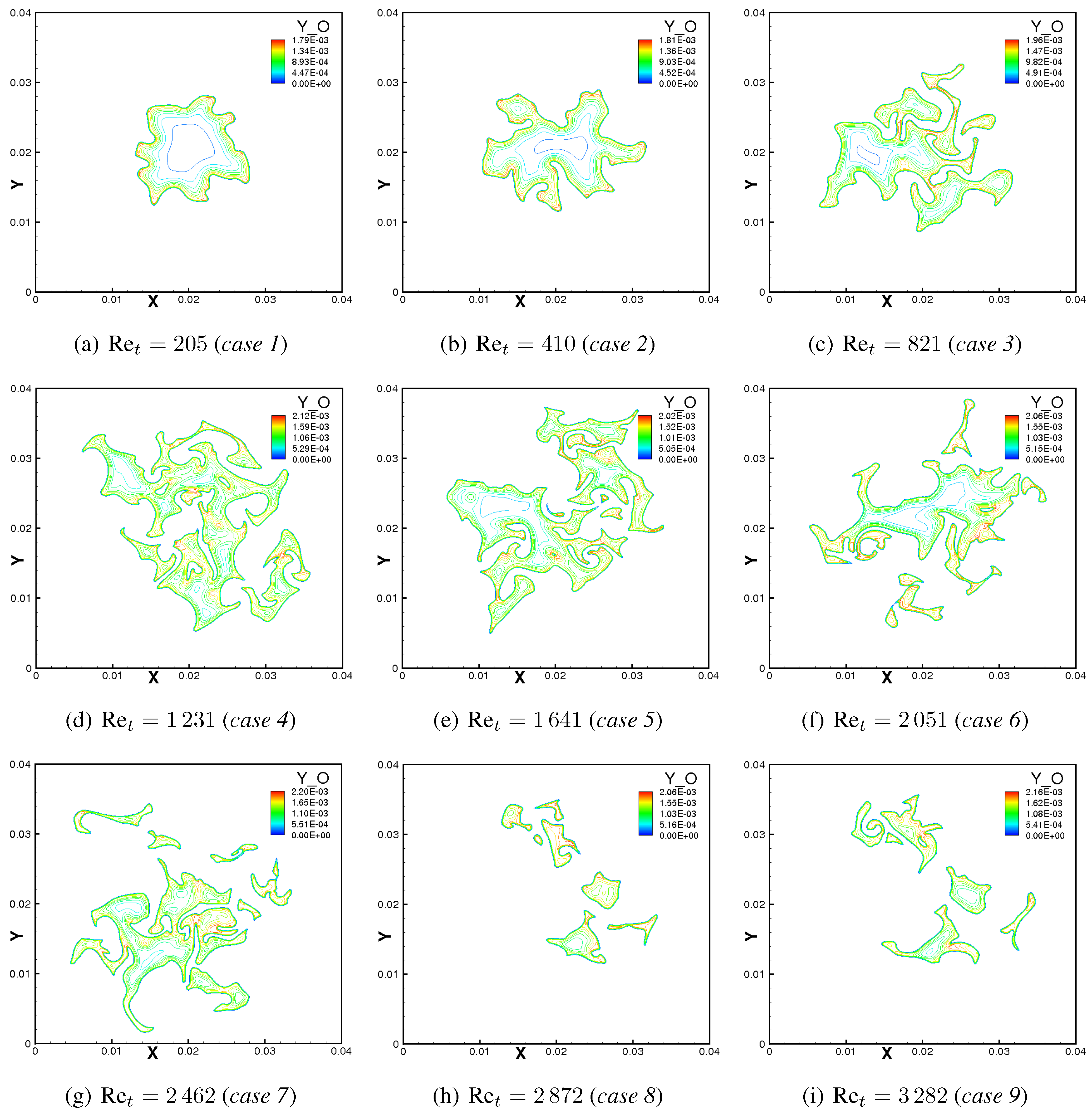
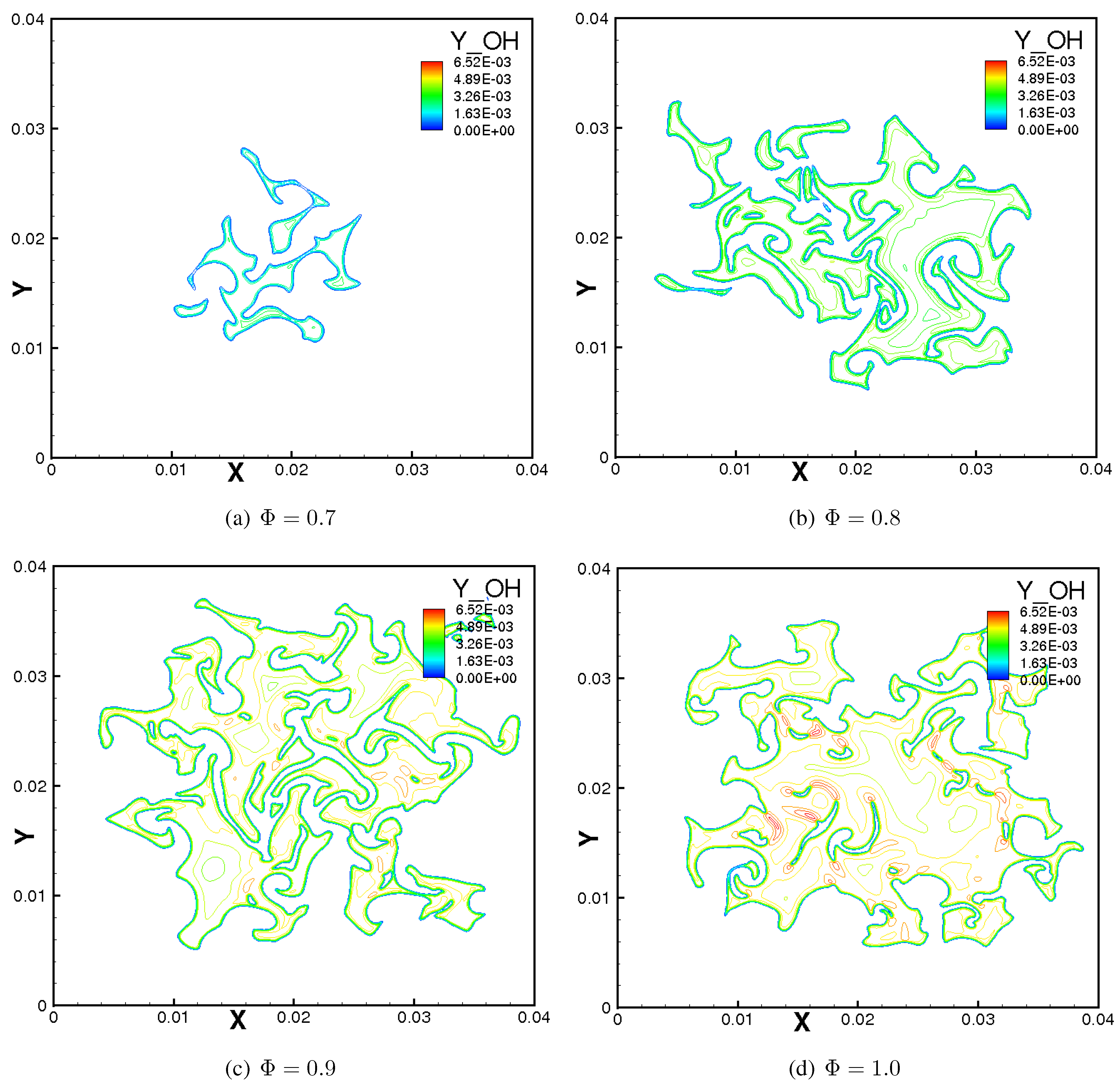
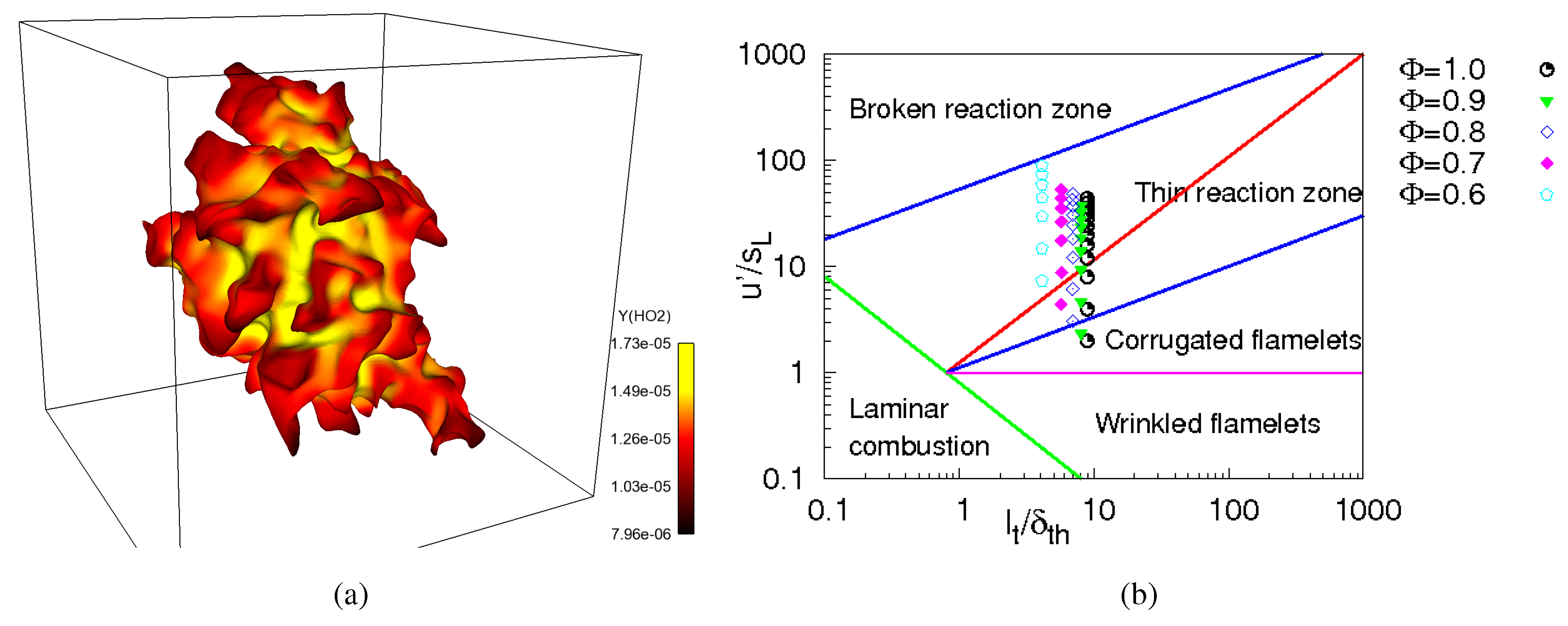
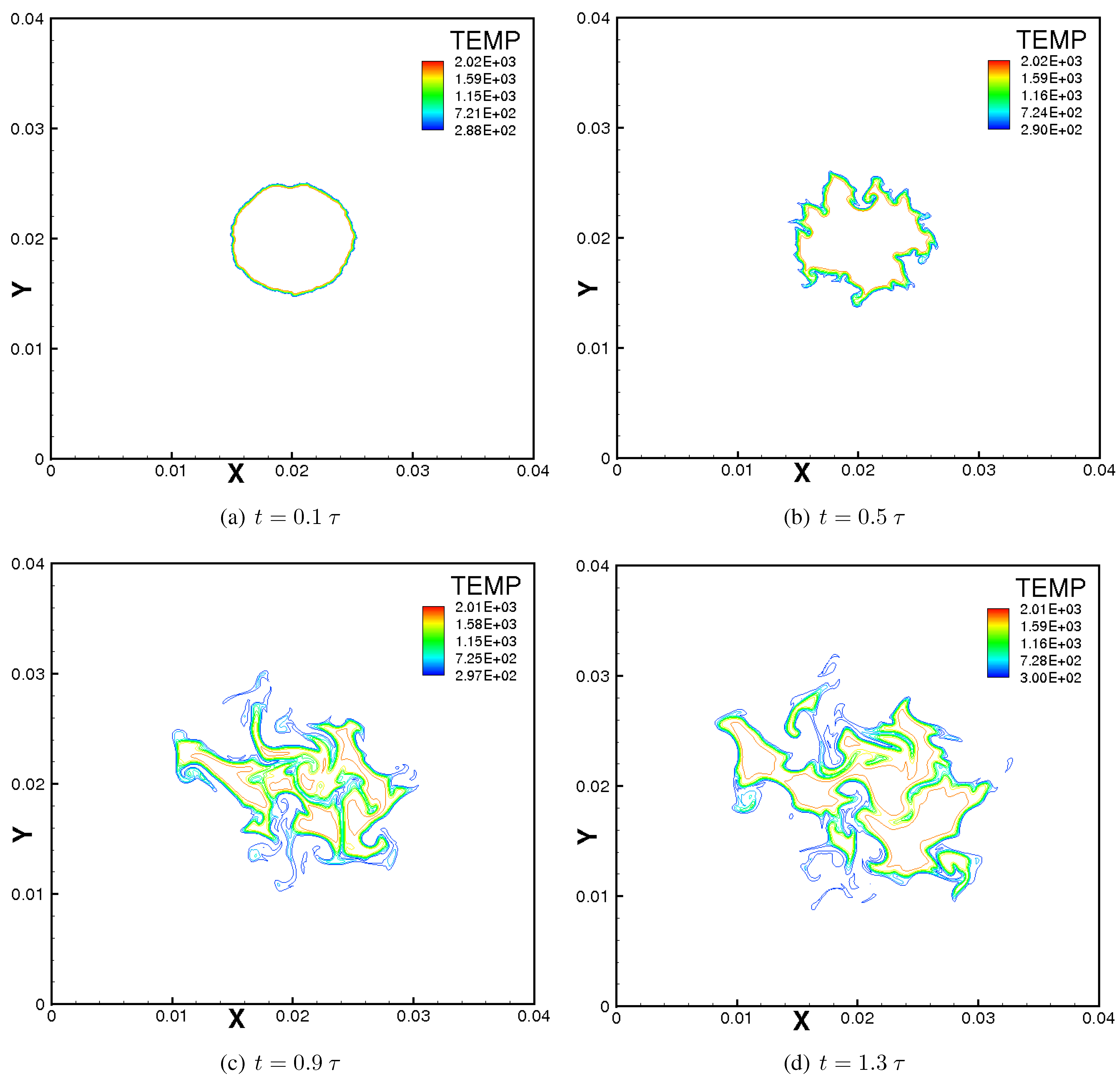
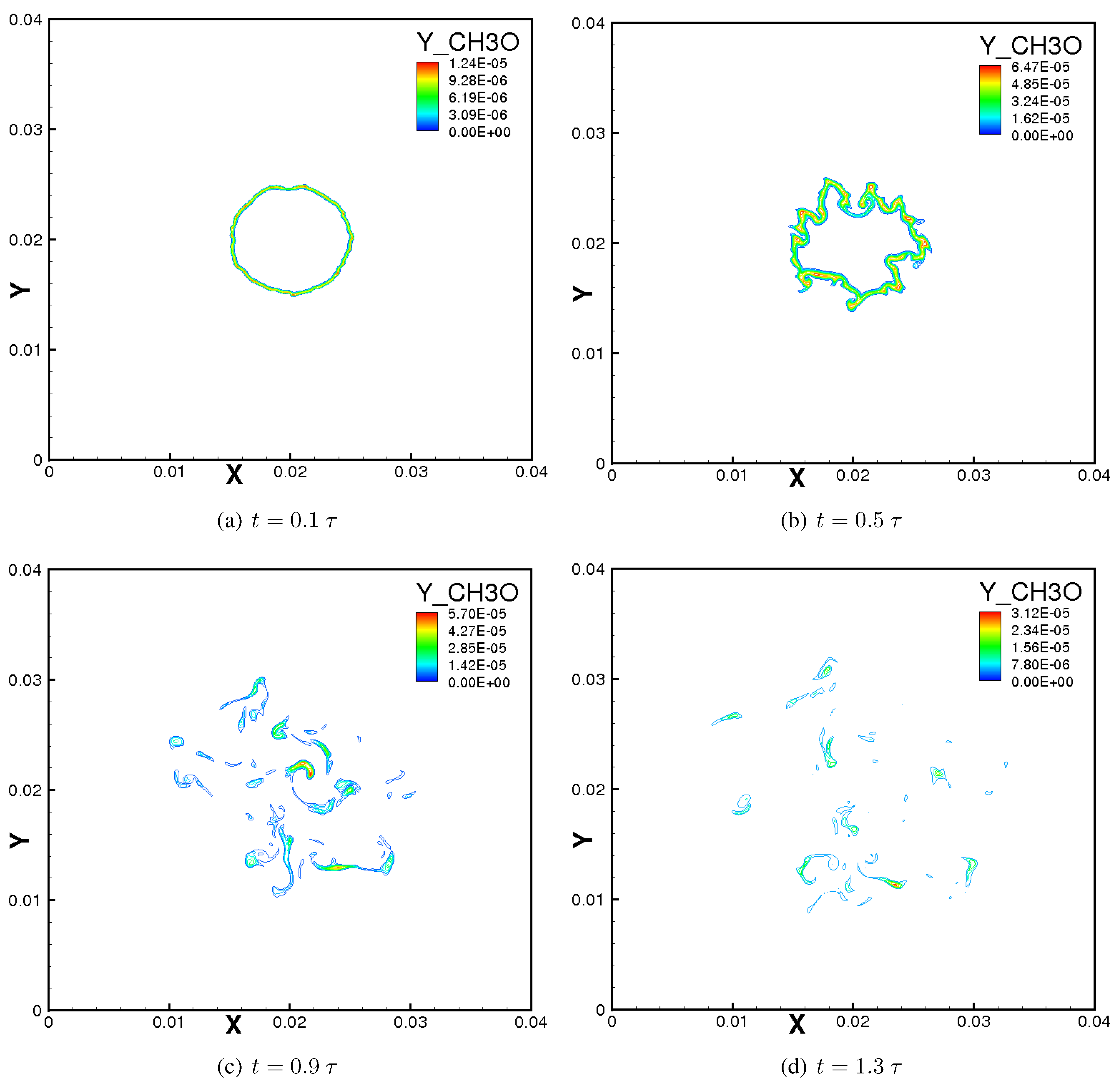
4.1. Turbulent Flame Structure

The effect of turbulence on the physical structure of the flame is first investigated visually by examining both the instantaneous and temporal evolution of the temperature and of selected species mass fraction fields, plotted in Figure 2, Figure 3, Figure 4 and Figure 5. All figures are cut in the middle plane $z=2.0$ cm.

Figure 2. Time evolution of the iso-contours of temperature (case 7, Re${}_t=2462$) for mixture equivalence ratio $\Phi =0.8$ at $t=0.1\tau$, $0.5\tau$, $0.9\tau$ and $1.3\tau$.

Figure 2. Time evolution of the iso-contours of temperature (case 7, Re${}_t=2462$) for mixture equivalence ratio $\Phi =0.8$ at $t=0.1\tau$, $0.5\tau$, $0.9\tau$ and $1.3\tau$.

Figure 2 and Figure 3 show the iso-contours of temperature and mass fraction of CH${}_3$O computed with the same mixture equivalence ratio $\Phi =0.8$ for case 7, illustrating the physical flame structure at different non-dimensional times $t=0.1\tau$, $0.5\tau$, $0.9\tau$ and $1.3\tau$. Considering the temperature field, the initial laminar spherical flame (Figure 2a) is progressively being distorted and stretched (Figure 2b) by the very strong turbulent field with time, leading to the creation of islands (in the form of both hot and fresh gas pockets) and edge flame-like structures (Figure 2c,d) [38] at various locations within the computational domain and for various shapes and sizes. For a high turbulence intensity, local flame extinction and flame-flame interactions become important.

Figure 3. Time evolution of the iso-contours of the mass fraction of CH${}_3$O (case 7, Re${}_t=2462$) for mixture equivalence ratio $\Phi =0.8$ at $t=0.1\tau$, $0.5\tau$, $0.9\tau$ and $1.3\tau$.

Figure 3. Time evolution of the iso-contours of the mass fraction of CH${}_3$O (case 7, Re${}_t=2462$) for mixture equivalence ratio $\Phi =0.8$ at $t=0.1\tau$, $0.5\tau$, $0.9\tau$ and $1.3\tau$.

The temporal evolution of the iso-contours of the minor radical CH${}_3$O is shown in Figure 3 for the same Φ and Re${}_t$ values.en The wrinkling effect induced by turbulence follows the patterns in the temperature field but shows much stronger disruptions at later times ($t=0.9$–$1.3\tau$). Such events are usually not observed when looking at integrated quantities, like temperature, illustrating the importance of a detailed description of chemical processes. Considering CH${}_3$O as a measure of flame activity, local extinction events can be tracked with a good temporal and spatial resolution. Numerous fresh gas islands and flame pinch-off events are visible (Figure 3c), evidencing local flame extinctions. Looking at the mass fraction values, the peak species mass fraction rises soon after its formation from $1.24\times {10}^{-5}$ at $t=0.1\tau$ to $6.47\times {10}^{-5}$ at $t=0.5\tau$, after which it drops to $5.76\times {10}^{-5}$ at $t=0.9\tau$, then down to $3.12\times {10}^{-5}$ at $t=1.3\tau$.

The iso-contours of most major and minor species exhibit qualitatively similar patterns to those of the temperature and CH${}_3$O fields, respectively. They are therefore not shown in the interest of space.

Figure 4. Instantaneous iso-surface of the mass fraction of O for different integral Reynolds number Re${}_t$ at the same mixture equivalence ratio $\Phi =0.9$ and same time $t=1.3\tau$.

Figure 4. Instantaneous iso-surface of the mass fraction of O for different integral Reynolds number Re${}_t$ at the same mixture equivalence ratio $\Phi =0.9$ and same time $t=1.3\tau$.

Snapshots of the iso-surface of the mass fraction of the oxygen atom is shown in Figure 4 for different Re${}_t$ values at the same time $t=1.3\tau$ and mixture ratio $\Phi =0.9$. In the past, DNS easily accessed mild turbulence conditions such as the one shown in Figure 4a–c where the flame is only slightly contorted. Comparing the snapshots in Figure 4, it is observed qualitatively that the amount of wrinkling increases strongly from Figure 4a–c and tends to saturate afterwards (compare in particular Figure 4d with Figure 4e). For higher values of Re${}_t$, considerable structural modifications are observed, in particular flame–flame interactions, leading to pinch off as evident in the higher Re${}_t$ snapshots in Figure 4c–e. The resulting turbulent flame structure is then marred with numerous perforations. Further increase in turbulence intensity leads to a further increase of pinch off and mutual annihilation effects, thereby limiting further increase in the flame surface area. Consequently, it drops steadily as evidenced in Figure 4f–i, indicating the growing importance of extinction processes, as also observed experimentally in combustion vessel experiments [2,39].

Figure 5. Instantaneous iso-contours of the mass fraction of OH (case 6, Re${}_t=2051$) for different mixture equivalence ratios Φ at the same time $t=1.3\tau$.

Figure 5. Instantaneous iso-contours of the mass fraction of OH (case 6, Re${}_t=2051$) for different mixture equivalence ratios Φ at the same time $t=1.3\tau$.

To show the effect of the equivalence ratio on the turbulent flame structure, Figure 5 presents the instantaneous iso-contours of the mass fraction of OH (case 6) for different mixture equivalence ratios $\Phi =0.7$, $0.8$, $0.9$ and $1.0$ at the same time $t=1.3\tau$. The color scale is kept identical for all plots. The lower flame activity when decreasing the equivalence ratio can easily be seen in this figure, explaining again why local flame extinction is systematically observed earlier at lower values of Φ. Since the employed chemical scheme has only been validated for lean to stoichiometric conditions, similar studies for rich conditions cannot be presented.

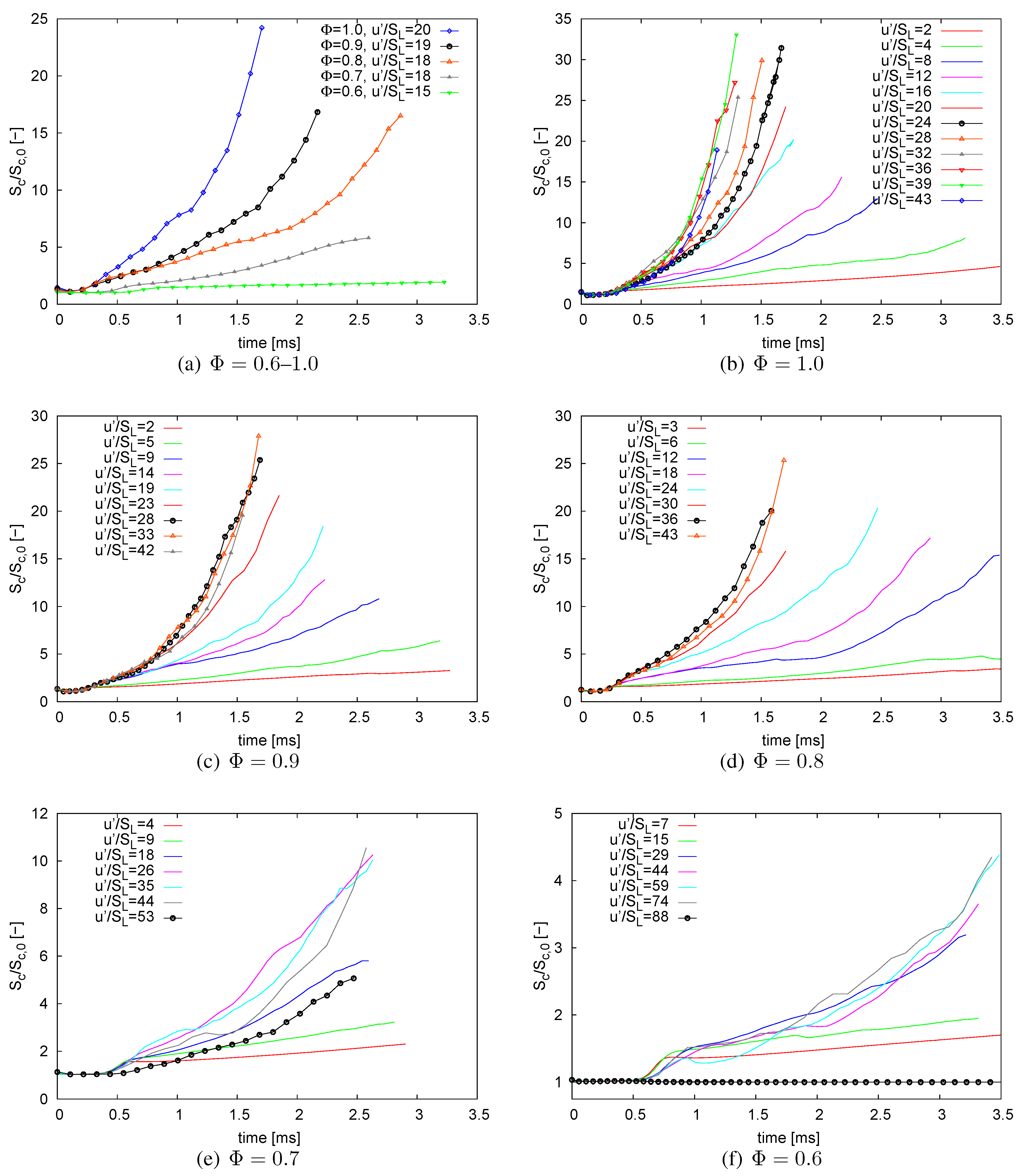
4.2. Turbulent Burning Velocity

Now, the time evolution of the turbulent burning velocity as a function of the turbulence intensity is investigated in moderate to intense turbulent flows for various Φ. Following [3], it is emphasized that different definitions of $S_T$ may be useful in different contexts. In the present simulations, the consumption speed $S_c$ is defined following [40] and computed as the volume integrated overall rate of fuel combustion per unit flame area (assuming complete fuel consumption on the burned gas side), in a similar manner as employed, for instance, in [41,42]:

$$S_c\propto -\frac{W_f}{{\rho }_f{Y}_f}\int {\dot{\omega }}_{f}dV$$

(7)

where $W_f$ is the fuel molecular weight and ${\rho }_f$ and $Y_f$ are the density and mass fraction of the fuel in the fresh gas mixture, respectively. The associated scaling area has been obtained in a post-processing step using AnaFlame [43]. It is chosen as the area of a suitable iso-contour of the reaction progress variable c, (defined following [44] in terms of reduced temperature) representing the wrinkled flame front. For instance, a choice of $c=0.6$, corresponding to the position of maximum heat release in the laminar flame could be adopted. Thus the value of $S_c$ is not unique. We note also that ensemble averaging would be needed to provide a mean isosurface scaling area, which could account further for flame wrinkling effects. The computed fuel consumption rate is then directly related to the overall burning rate (by scaling with this area), and constitutes an interesting measure of the burning velocity. In all results shown, $S_c$ is scaled by its initial value $S_{c,0}(t=0)$ (before starting the interaction with the prescribed field of turbulence) at the corresponding equivalence ratio.

This global flame parameter is of primary importance to burner designers as far as the characterization of premixed turbulent combustion is concerned. Its prediction remains a challenge for turbulent premixed combustion modelers [45]. Most existing models are still phenomenological in nature and often fail beyond the flammability limits, whenever the pre-mixture is either too lean or too rich to sustain a flame in the mean.

The temporal evolution of the consumption speed is shown in Figure 6 for the various cases. Initially, it remains nearly constant up to $t\approx 0.3$ ms and $t\approx 0.6$ ms for $\Phi =1.0$ and $\Phi =0.6$, respectively, after which it increases steadily. Under the same flow conditions, the time required by the leaner mixtures to sustain and propagate a flame front is delayed relative to the richer ones, as expected. After a successful take-off, the profiles for the various cases take different courses depending on the turbulence intensity $u^{\prime }$, mostly with a steady increase in slope. For a given value of $u^{\prime }/S_L$ (which is the parameter mostly used for modeling purposes), the gradient of the profiles increases with increasing Φ as shown in Figure 6a,

Figure 6. Temporal evolution of the volume-integrated fuel (CH${}_4$) consumption rate $S_c$ (normalized by their laminar flame value at the corresponding equivalence ratio and at $t=0$) for different turbulence intensities $u^{\prime }/S_L$ and mixture equivalence ratios Φ .

Figure 6. Temporal evolution of the volume-integrated fuel (CH${}_4$) consumption rate $S_c$ (normalized by their laminar flame value at the corresponding equivalence ratio and at $t=0$) for different turbulence intensities $u^{\prime }/S_L$ and mixture equivalence ratios Φ .

where all the profiles for the five mixture compositions are plotted together for a nearly constant value of $u^{\prime }/S_L$. Also, it is obvious that the leaner the mixture, the lower the fuel consumption rate and vice versa. Note the progressive exponential nature of the curves associated with the richer mixtures ($\Phi \ge 0.9$) under highly turbulent conditions. However, as the turbulence intensity further increases, a maximum in $S_c$ is observed. This critical (or saturation) rms velocity will be denoted $u_s^{\prime }$. As found in the DNS, the richer the mixture, the higher the scaled saturation velocity: $u_s^{\prime }/S_L$ is about $29.0$ for $\Phi =0.6$ and up to $39.0$ at stoichiometry. Increasing $u^{\prime }$ beyond $u_s^{\prime }$, the obtained temporal profiles of $S_c$ first cluster together (e.g., Figure 6b & c for $\Phi =1.0$ & $0.9$) before declining steadily (e.g., Figure 6d & e for $\Phi =0.8$ & $0.7$). This scenario is a well known phenomena observed in several combustion vessel experiments and termed “bending effect” [44,46]. Whether such a decline persist until the flame reaches global quenching (the so called "quenching limit", also observed in many experiments) for too intense turbulence, will be the subject of further studies. Figure 6f includes a case for which, due to a high initial turbulence level ($u_s^{\prime }/S_L=88$), the pre-mixture is unable to propagate and slowly fades out. The present DNS results thus confirm the theoretical and experimental assertions that turbulence cannot increase burning rates indefinitely [7,9]. Furthermore, leaner methane–air mixtures (e.g., $\Phi =0.6$ at $u^{\prime }/S_L\ge 74.0$) exhibit a greater decline in $S_c$ with increasing $u^{\prime }/S_L$ than do richer ones.

Since high volumetric heat release rates in compact burners at low stoichiometries are often required, combustion in a highly turbulent medium is often necessary [47]. Intense turbulence stirring usually results in flames that burn and/or propagate faster and release higher amounts of energy in the form of heat. However, the obtained results show that optimum conditions exist, depending on mixture stoichiometry, above which the resulting flames will be weakened by a further increase in turbulent stirring.

5. Concluding Remarks

Direct Numerical Simulations have been realized in a parametric study in order to investigate the response of turbulent consumption speed described by the fuel consumption rate for premixed methane–air combustion. Five different mixture equivalence ratios Φ have been considered, each for increasing values of the integral Reynolds number. Highly turbulent conditions (Re${}_t$ up to $4513$) have been accessed for each Φ and the effect of turbulence on the physical structure of the flame has been investigated. Local flame quenching has been observed within the computational domain. Quenching effects appear earlier with the leaner mixtures, as expected. Profiles of the fuel consumption rate rise steadily with increasing turbulence intensity till a saturation rms velocity is reached, beyond which the time evolutions collapse together before decreasing steadily. These DNS results confirm qualitatively theoretical and experimental findings from the literature regarding the correlation between scaled turbulence intensity $u^{\prime }/S_L$ and turbulent flame speed quantified by $S_c$ [44]: $S_c$ first increases, roughly linearly, with $u^{\prime }/S_L$ (low turbulence zone) and then levels off (bending zone). For a fixed value of $u^{\prime }/S_L$, which already incorporates compositional variations, values of $S_c/S_L$ still appear to depend on the mixture equivalence ratio. As a consequence, simplified phenomenological expressions relating $S_c/S_L$ simply to $u^{\prime }/S_L$ should probably also take into account the influence of further parameters [3].

Assuming a generic relation in the form $S_c/S_L={[1+C{(u^{\prime }/S_L)}^n]}^{1/n}$ [48], the model constants C and n are found to be $\approx 0.25$ and $\approx 1.16$, respectively, from fits of the DNS data of $S_c/S_L$ for single runs, in comparison with experimental estimations of $0.45$ and $1.0$ [47]. The DNS data are presently extended in order to propose quantitative correlations that might be used in turbulent combustion models with a sufficient level of generality. Ensemble averaging should also be conducted in order to obtain ultimately a statistically significant analysis of the results [49]. This ensure that a mean isosurface area of c is employed in conjunction with Equation 7 in order to account for flame wrinkling effects.

References

1. Abdel-Gayed, R.; Bradley, D.; Lawes, M.; Lung, F. Premixed turbulent burning during explosions. Proc. Combust. Inst. 1986, 21, 497–504. [Google Scholar] [CrossRef]
2. Abdel-Gayed, R.; Bradley, D.; Lawes, M. Turbulent burning velocities: A general correlation in terms of straining rates. Proc. R. Soc. Lond. 1987, A414, 389–413. [Google Scholar] [CrossRef]
3. Driscoll, J. Turbulent premixed combustion: Flamelet structure and its effects on turbulent burning velocities. Prog. Energy Combust. Sci. 2008, 34, 91–134. [Google Scholar] [CrossRef]
4. Peters, N. The turbulent burning velocity for large-scale and small-scale turbulence. J. Fluid Mech. 1999, 384, 107–132. [Google Scholar] [CrossRef]
5. Abdel-Gayed, R.; Bradley, D. Criteria for turbulent propagation limits of premixed flames. Combust. Flame 1985, 62, 61–68. [Google Scholar] [CrossRef]
6. Kozachenko, L.; Kuznetsov, I. Burning velocity in a turbulent stream of a homogeneous mixture. Combust. Explos. Shock Waves 1965, 1, 22–30. [Google Scholar] [CrossRef]
7. Bradley, D. How fast can we burn? Proc. Combust. Inst. 1993, 24, 247–262. [Google Scholar] [CrossRef]
8. Shy, S.; Jang, R.; Tang, C. Simulation of turbulent burning velocities using aqueous autocatalytic reactions in a near-homogeneous turbulence. Combust. Flame 1996, 105, 54–62. [Google Scholar] [CrossRef]
9. Shy, S.; Lin, W.; Wei, J. An experimental correlation of turbulent burning velocities for premixed turbulent methane—air combustion. Proc. R. Soc. Lond. 2000, 456, 1997–2019. [Google Scholar] [CrossRef]
10. Shy, S.; Lin, W.; Peng, K. High-intensity turbulent premixed combustion: General correlations of turbulent burning velocities in a new cruciform burner. Proc. Combust. Inst. 2000, 28, 561–568. [Google Scholar] [CrossRef]
11. Cant, S. Direct Numerical Simulation of premixed turbulent flames. Philos. Trans. R. Soc. A Lond. 1999, 357, 3583–3604. [Google Scholar] [CrossRef]
12. Yaldizli, M.; Mehravaran, K.; Mohammad, H.; Jaberi, F. The structure of partially premixed methane flames in high-intensity turbulent flows. Combust. Flame 2008, 154, 692–714. [Google Scholar] [CrossRef]
13. Jenkins, K.; Cant, R. Curvature effects on flame kernels in a turbulent environment. Proc. Combust. Inst. 2002, 29, 2023–2029. [Google Scholar] [CrossRef]
14. Haworth, D.; Blint, R.; Cuenot, B.; Poinsot, T. Numerical simulations of turbulent propane-air combustion with nonhomogenous reactants. Combust. Flame 2000, 121, 395–417. [Google Scholar] [CrossRef]
15. Bell, J.; Day, M.; Grcar, J. Numerical Simulation of Premixed Turbulent Methane Combustion. Proc. Combust. Inst. 2002, 29, 1987–1993. [Google Scholar] [CrossRef]
16. Chen, J.H.; Choudhary, A.; de Supinski, B.; DeVries, M.; Hawkes, E.R.; Klasky, S.; Liao, W.K.; Ma, K.L.; Mellor-Crummey, J.; Podhorszki, N.; et al. Terascale direct numerical simulations of turbulent combustion using S3D. Comput. Sci. Discov. 2009, 2, 31. [Google Scholar] [CrossRef]
17. Tanahashi, M.; Nada, Y.; Ito, Y.; Miyauchi, T. Local flame structure in the well stirred reactor regime. Proc. Combust. Inst. 2002, 29, 2041–2049. [Google Scholar] [CrossRef]
18. Sankaran, R.; Hawkes, E.; Chen, J. Structure of a spatially developing turbulent lean methane-air Bunsen flame. Proc. Combust. Inst. 2006, 31, 1291–1298. [Google Scholar] [CrossRef]
19. Bell, J.; Day, M.; Shepherd, I.; Johnson, M.; Cheng, R.; Grcar, J.; Beckner, V.; Lijewski, M. Numerical Simulation of a laboratory scale turbulent V-flame. Proc. Natl. Acad. Sci. USA 2005, 102, 10006–10011. [Google Scholar] [CrossRef] [PubMed]
20. Bell, J.; Day, M.; Grcar, J.; Lijewski, M.; Driscoll, J.; Filatyev, S. Numerical simulation of a laboratory-scale turbulent slot flame. Proc. Combust. Inst. 2007, 31, 1299–1307. [Google Scholar] [CrossRef]
21. Veynante, D.; Vervisch, L. Turbulent combustion modeling. Prog. Energy Combust. Sci. 2002, 28, 193–266. [Google Scholar] [CrossRef]
22. Thévenin, D.; Behrendt, F.; Maas, U.; Przywara, B.; Warnatz, J. Development of a parallel direct simulation code to investigate reactive flows. Comput. Fluids 1996, 25, 485–496. [Google Scholar] [CrossRef]
23. Kee, R.; Miller, J.; Jefferson, T. Chemkin, a General Purpose Problem-Independent Transportable FORTRAN Chemical Kinetics Code Package; Technical Report SAND80-8003; Sandia National Laboratry: Albuquerque, NM, USA, 1980. [Google Scholar]
24. Ern, A.; Giovangigli, V. Eglib Server and User’s Manual. Available online: http://www.cmap.polytechnique.fr/www.eglib (accessed on 1 June 2009).
25. Kuo, K. Principles of Combustion; John Wesley & Sons, Inc.: New York, NY, USA, 2005. [Google Scholar]
26. Laverdant, A. Notice d’utilisation du Programme SIDER (PARCOMB3D); Technical Report RT 2/13635 DEFA; The French Aerospace Laboratry, ONERA: Chatillon, French, 2008. [Google Scholar]
27. Fru, G.; Janiga, G.; Thévenin, D. Direct Numerical Simulation of highly turbulent premixed flames burning methane. In Direct and Large-Eddy Simulation VIII; Kuerten, H., Ed.; ERCOFTAC Series; Springer-Verlag: Eindhoven, The Netherlands, 2011; pp. 327–332. [Google Scholar]
28. Fru, G.; Janiga, G.; Thévenin, D. Simulation of turbulent combustion processes under realistic conditions. In DEISA Digest 2011; Turunen, A., Lederer, H., Autio, T., Pyysalo, S., Morgan, N., Rötkönen, P., Eds.; Extreme Computing in Europe Series; DEISA Media: Garching, Germany, 2011; pp. 20–22. [Google Scholar]
29. Honein, A.; Moin, P. Higher entropy conservation and numerical stability of compressible turbulence simulations. J. Comput. Phys. 2004, 201, 531–545. [Google Scholar] [CrossRef]
30. Baum, M.; Poinsot, T.; Thévenin, D. Accurate boundary conditions for multicomponent reactive flows. J. Comput. Phys. 1995, 116, 247–261. [Google Scholar] [CrossRef]
31. Hilbert, R.; Thévenin, D. Influence of differential diffusion on maximum flame temperature in turbulent nonpremixed hydrogen/air flames. Combust. Flame 2004, 138, 175–187. [Google Scholar] [CrossRef]
32. Klein, M.; Sadiki, A.; Janicka, J. A digital filter based generation of inflow data for spatially developing direct numerical or large eddy simulations. J. Comput. Phys. 2003, 186, 652–665. [Google Scholar] [CrossRef]
33. Kempf, A.; Klein, M.; Janicka, J. Efficient generation of initial and inflow-conditions for transient flows in arbitrary geometries. Flow Turbul. Combust. 2005, 74, 67–84. [Google Scholar] [CrossRef]
34. Smooke, M.D.; Giovangigli, V. Formulation of the premixed and nonpremixed test problems. In Reduced Kinetic Mechanism and Asymptotic Approximations for Methane-Air Flames; Smooke, M.D., Ed.; Springer-Verlag: New York, NY, USA, 1991; Volume 384, pp. 1–28. [Google Scholar]
35. James, S.; Jaberi, F. Large scale simulations of two-dimensional nonpremixed methane jet flames. Combust. Flame 2000, 123, 465–487. [Google Scholar] [CrossRef]
36. Fru, G.; Janiga, G.; Thévenin, D. Direct Numerical Simulation of turbulent methane flames with and without volume viscosity. In 8th Euromech Fluid Mechanics Conference (EFMC-8), Munich, Germany, 13–16 September 2010. paper MS2–9.
37. Rutland, C.; Ferziger, J.; El-Thary, S. Full numerical simulations and modeling of turbulent premixed flames. Proc. Combust. Inst. 1990, 23, 621–627. [Google Scholar] [CrossRef]
38. Bédat, B.; Egolfopoulos, F.; Poinsot, T. Direct Numerical Simulation of heat release and NOx formation in turbulent non premixed flames. Combust. Flame 1999, 119, 69–83. [Google Scholar] [CrossRef]
39. Abdel-Gayed, R.; Al-khishali, K.; Bradley, D. Turbulent Burning Velocities and Flame Straining in Explosions. Proc. R. Soc. Lond. 1984, A391, 393–414. [Google Scholar] [CrossRef]
40. Poinsot, T.; Echekki, T.; Mungal, M. A study of the laminar flame tip and implications for premixed turbulent combustion. Combust. Sci. Technol. 1992, 81, 45–73. [Google Scholar] [CrossRef]
41. Im, H.; Chen, J. Effects of flow transients on the burning velocity of laminar hydrogen/air premixed flames. Proc. Combust. Inst. 2000, 28, 1833–1840. [Google Scholar] [CrossRef]
42. Sankaran, R.; Im, H. Effect of hydrogen addition on the flammability limit of stretched methane/air premixed flames. In Proceedings of the Third Joint Meeting of the U.S. Section of the Combustion Institute, Chicago, IL, USA, March 2003; pp. 1–6.
43. Zistl, C.; Hilbert, R.; Janiga, G.; Thévenin, D. Increasing the efficiency of post-processing for turbulent reacting flows. Comput. Visual. Sci. 2009, 12, 383–395. [Google Scholar] [CrossRef]
44. Poinsot, T.; Veynante, D. Theoretical and Numerical Combustion, 2nd ed.; R.T. Edwards, Inc.: Philadelphia, PA, USA, 2005. [Google Scholar]
45. Warnatz, J.; Maas, U.; Dibble, R.W. Combustion: Physical and Chemical Fundamentals, Modeling and Simulations, Experiments, Pollutant Formation, 3rd ed.; Springer: Berlin, Germany, 2001. [Google Scholar]
46. Abdel-Gayed, R.; Bradley, D.; Hamid, N.; Lawes, M. Lewis number effects on turbulent burning velocity. Proc. Combust. Inst. 1985, 20, 505–512. [Google Scholar] [CrossRef]
47. Shepherd, I.; Cheng, R. The burning rate of premixed flames in moderate and intense turbulence. Combust. Flame 2001, 127, 2066–2075. [Google Scholar] [CrossRef]
48. Pocheau, A. Front propagation in a turbulent medium. Europhys. Lett. 1992, 20, 404–406. [Google Scholar] [CrossRef]
49. Shalaby, H.; Thévenin, D. Statistically significant results for the propagation of a turbulent flame kernel using direct numerical simulation. Flow Turbul. Combust. 2010, 84, 357–367. [Google Scholar] [CrossRef]