SVR with Hybrid Chaotic Immune Algorithm for Seasonal Load Demand Forecasting

Abstract

Accurate electric load forecasting has become the most important issue in energy management; however, electric load demonstrates a seasonal/cyclic tendency from economic activities or the cyclic nature of climate. The applications of the support vector regression (SVR) model to deal with seasonal/cyclic electric load forecasting have not been widely explored. The purpose of this paper is to present a SVR model which combines the seasonal adjustment mechanism and a chaotic immune algorithm (namely SSVRCIA) to forecast monthly electric loads. Based on the operation procedure of the immune algorithm (IA), if the population diversity of an initial population cannot be maintained under selective pressure, then IA could only seek for the solutions in the narrow space and the solution is far from the global optimum (premature convergence). The proposed chaotic immune algorithm (CIA) based on the chaos optimization algorithm and IA, which diversifies the initial definition domain in stochastic optimization procedures, is used to overcome the premature local optimum issue in determining three parameters of a SVR model. A numerical example from an existing reference is used to elucidate the forecasting performance of the proposed SSVRCIA model. The forecasting results indicate that the proposed model yields more accurate forecasting results than the ARIMA and TF-ε-SVR-SA models, and therefore the SSVRCIA model is a promising alternative for electric load forecasting.

1. Introduction

As the development of the economy is vigorously proceeds, ensuring that electric energy is available for all electricity users whenever and wherever needed (i.e., meeting users’ demands) will be an important challenge for the electric energy industry. Therefore, accurate electric load forecasting is vital not only for the energy transactions in a competitive electricity market [1], but also for those resource-constrained developing countries (like Taiwan) where the capability to import and export electricity is limited [2]. However, prediction of the electric load is a complex problem, because it is influenced by various factors, including climatic factors, social activities, and seasonal factors. Climate factors depend on the temperature and humidity; social factors imply human social activities including work, school and entertainment activities affecting the electric load; seasonal factors then include seasonal climate changes and load growth year after year.

There are widespread references with regard to the efforts improving the accuracy of forecasting methods. One of these methods is a weather-insensitive approach which used historical load data to infer the future electric load. It is famous known as Box-Jenkins’ ARIMA [3,4,5], which is a weather-insensitive approach that uses historical load data to infer the future electric load. In addition, Christianse [6] and Park et al. [7] have proposed exponential smoothing models by employing Fourier series transformation to forecast electric loads. The disadvantage of these methods is that they are time consuming, particularly for the situation while the number of variables is increased. State space and Kalman filtering technologies, developed to reduce the difference between actual loads and prediction loads (random error), are employed in load forecasting models. This approach introduces the periodic component of load as a random process. It requires historical data for more than 3- to 10-years to construct the periodic load variation and to estimate the dependent variables (load or temperature) of power system [8,9,10]. The disadvantage of these methods is that it is difficult to avoid the observation noise in the forecasting process, especially when multiple variables are considered. Regression models construct causal-effect relationships between electric load and independent variables. The most popular models are linear regression, proposed by Asbury [11], considering the “weather” variable into forecasting model. Papalexopoulos and Hesterberg [12] added the factors of “holiday” and “temperature” into their proposed model. The proposed model used a weighted least squares method to obtain robust parameter estimation encountering heteroskedasticity. Soliman et al. [13] proposed a multivariate linear regression model in load forecasting, including temperature, wind cooling/humidity factors. Their empirical results indicate that the proposed model outperforms the harmonic model as well as the hybrid model. These models are based on linear assumptions, but the use of these independent variables is unjustified because of the terms are known to be nonlinear.

In the recent decade, lots of researchers have tried to apply artificial intelligence techniques to improve the accuracy of the load forecasting. Knowledge-based expert systems (KBES’) and artificial neural networks (ANNs) are the popular representatives. The KBES approaches performed electric load forecasting by simulating the experiences of system operators who were well-experienced in the electricity generation processes, such as Rahman and Bhatnagar [14]. The characteristic feature of this approach is that it is rule-based, which implies that the system transforms new rules from received information. In other words, it is presumed that an expert trained using existing data will provide increased forecasting accuracy [14,15,16]. This approach is a derivation of the rules from on-the-job training and sometimes transforming the information logic into equations could be impractical. Lots of researchers have also tried to apply ANNs to improve the load forecasting accuracy. Park et al. [17] proposed a 3-layer back-propagation neural network for daily load forecasting problems. The inputs include three indices of temperature: average, peak and lowest loads. The outputs are peak loads. The proposed model outperforms the regression model and the time series model in terms of forecasting accuracy index and mean absolute percent error (MAPE). Novak [18] applied radial basis function (RBF) neural networks to forecasting electricity loads. The results indicate that RBF is at least 11 times faster and more reliable than back-propagation neural networks. Darbellay and Slama [19] applied ANNs to predict the electricity load in the Czech Republic. The experimental results indicate that the proposed ANN model outperformed the ARIMA model in terms of forecasting accuracy index, normalized mean square error (NMSE). Abdel-Aal [20] proposed an Abductive network to conduct one-hour-ahead load forecasting for five years. Hourly temperature and hourly load data are considered. The results of the proposed model are very promising in terms of forecasting accuracy index, MAPE. Hsu and Chen [21] employed the ANN model to forecast the regional electricity load in Taiwan. The empirical results indicate that proposed model is superior to the traditional regression model. However, it is possible to get trapped in local minima and be subjective in selecting the model architecture [22].

Support vector machines (SVM) were originally developed to solve pattern recognition and classification problems. With the introduction of Vapnik’s ε-insensitive loss function, SVMs have been extended to solve nonlinear regression estimation problems, i.e., the so-called support vector regression (SVR), and have been successfully applied to solve forecasting problems in many fields such as financial time series (stocks indexes and exchange rates) forecasting [23,24,25,26,27], tourist arrival forecasting [28,29], the engineering and software field (production values and reliability forecasting) [30,31], atmospheric science forecasting [32,33,34,35], and so on. Meanwhile, the SVR model has also been successfully applied to forecasting electric loads [36,37,38,39,40,41]. The practical results indicated that poor forecasting accuracy suffered from the lack of knowledge of the selection of the three parameters (σ, C, and ε) in a SVR model. However, the structured ways for determining three free parameters in a SVR model are poor. Recently, some major nature-inspired evolutionary algorithms were applied to solve optimization problems, the immune algorithm (IA) being one of them. IA, proposed by Mori et al. [42] and used in this study, is based on the learning mechanism of natural immune systems. Similar to GA, SA, and PSO, IA is also a population based evolutionary algorithm, therefore, it provides a set of solutions for exploration and exploitation of search space to obtain optimal/near optimal solutions [43]. In addition, the diversity of the employed population set will determine the search results, the desired solution or premature convergence (trapping in a local minimum). To overcome these drawbacks, it is necessary to find some effective approaches and improvements of the IA to maintain the population diversity and avoid leading to a local optimum. One possible approach is to divide the chromosome population into several subgroups and limit the crossover between the members in different subgroups to maintain the population diversity. However, such a method would require a huge population size, which is not typical in business forecasting application problem solving. Another feasible approach is focused on the chaos approach, due to its easy implementation and special ability to avoid being trapped in local optima [44]. Chaos often occurrs in a deterministic nonlinear dynamic system [45,46]. It is highly unstable motion in finite phase space. Such a motion is very similar to a random process (“randomicity”). Therefore, any variable in the chaotic space can travel ergodically over the whole space of interest (“ergodicity”). The variation of those chaotic variables obeys delicate inherent rules in spite of the fact that its variation may look like being in disorder (“regularity”). In addition, it is extremely sensitive to the initial conditions, which is an important property sometimes referred to as the so-called butterfly effect [47]. Attempting to simulate numerically a global weather system, Lorenz discovered that minute changes in initial conditions steered subsequent simulations towards radically different final states. Based on the two advantages of the chaos, the chaotic optimization algorithm (COA) was proposed to solve complex function optimizations [45]. The basic idea of the COA is to transform the problem variables from the solution space to the chaos space and then perform searches to find out the solution based on the three characteristics (randomicity, ergodicity, and regularity) of the chaotic variables. In this investigation, the chaotic immune algorithm (CIA) is tried to determine the values of three parameters in a SVR model. On the other hand, as indicated in the literature [48,49,50], electric energy demands also demonstrate a cyclic (seasonal) trend caused by the differences in demand from month to month and season to season, and the applications of SVR models to deal with cyclic (seasonal) trend time series, however, have not been widely explored. Therefore, this paper also attempts to apply the seasonal adjustment method [50,51] to deal with seasonal trend time series problems. The proposed SSVRCIA model is dedicated to improve forecasting performance in capturing non-linear and seasonal electric load changes tendencies. Two other forecasting approaches, the ARIMA and TF-ε-SVR-SA models proposed by Wang et al. [50], are used to compare the forecasting accuracy of electric load. The rest of this paper is organized as follows: the SSVRCIA model, including the formulation of SVR, the CIA algorithm, and the seasonal adjustment process, is introduced in Section 2. A numerical example is presented in Section 3. Conclusions are discussed in Section 4.

2. Methodology of the SSVRCIA Model

2.1. Support Vector Regression (SVR) Model

The brief basic concepts of SVMs for the case of regression are introduced. A nonlinear mapping $\phi (\cdot ):\hspace{1em}{\Re }^n\to {\Re }^{n_h}$ is defined to map the input data (training data set) ${\left\{(x_i,y_i)\right\}}_{i=1}^N$ into a so-called high dimensional feature space (which may have infinite dimensions), ${\Re }^{n_h}$. Then, in the high dimensional feature space, there theoretically exists a linear function, ƒ, to formulate the nonlinear relationship between input data and output data. Such a linear function, namely SVR function, is as Equation 1:

$$f(x)=w^{\text{T}}\phi (x)+b$$

(1)

where $f(x)$ denotes the forecasting values; the coefficients w ($w\in {\Re }^{n_h}$) and b ($b\in \Re$) are adjustable. SVR method aims at minimizing the empirical risk as Equation 2:

$$R_{emp}(f)=\frac{1}{N}{\displaystyle \sum _{i=1}^N{\Theta }_{\epsilon }(y_i,w^T\phi (x_i)+b)}$$

(2)

where ${\Theta }_{\epsilon }(y_i,w^T\phi (x_i)+b)$ is the ε-insensitive loss function and defined as Equation 3:

$${\Theta }_{\epsilon }(y_i,w^T\phi (x_i)+b)=\{\begin{array}{cc}\left|w^T\phi (x_i)+b-y_i\right|-\epsilon ,& if\begin{array}{}\end{array}\left|w^T\phi (x_i)+b-y_i\right|\ge \epsilon \\ 0,& otherwise\end{array}$$

(3)

In addition, ${\Theta }_{\epsilon }(y_i,w^T\phi (x_i)+b)$ is employed to find out an optimum hyperplane on the high dimensional feature space to maximize the distance separating the training data into two subsets. Thus, the SVR focuses on finding the optimum hyper plane and minimizing the training error between the training data and the ε-insensitive loss function. Then, the SVR minimizes the overall errors:

$$\underset{w,b,{\xi }^{*},\xi }{\text{Min}}{R}_{\epsilon }(w,{\xi }^{*},\xi )=\frac{1}{2}{w}^{\text{T}}w+C{\displaystyle \sum _{i=1}^N({\xi }_i^{*}+{\xi }_i)}$$

(4)

with the constraints:

$$\begin{array}{ll}{y}_i-w^{\text{T}}\phi (x_i)-b\le \epsilon +{\xi }_i^{*},\hfill & i=1,2,\mathrm{...},N\hfill \\ -y_i+w^{\text{T}}\phi (x_i)+b\le \epsilon +{\xi }_i,\hfill & i=1,2,\mathrm{...},N\hfill \\ {\xi }_i^{*}\ge 0,\hfill & i=1,2,\mathrm{...},N\hfill \\ {\xi }_i\ge 0,\hfill & i=1,2,\mathrm{...},N\hfill \end{array}$$

The first term of Equation 4, employing the concept of maximizing the distance of two separated training data, is used to regularize weight sizes, to penalize large weights, and to maintain regression function flatness. The second term penalizes training errors of $f(x)$ and y by using the ε-insensitive loss function. C is a parameter to trade off these two terms. Training errors above $\epsilon$ are denoted as ξ_i, whereas training errors below-ε are denoted as ξ_i.

After the quadratic optimization problem with inequality constraints is solved, the parameter vector w in Equation 1 is obtained from:

$$w={\displaystyle \sum _{i=1}^N\left({\beta }_i^{*}-{\beta }_i\right)\phi (x_i)}$$

(5)

where ${\beta }_i^{*}$, ${\beta }_i$ are obtained by solving a quadratic program and are the Lagrangian multipliers. Finally, the SVR regression function is obtained as Equation 6 in the dual space:

$$f(x)={\displaystyle \sum _{i=1}^N\left({\beta }_i^{*}-{\beta }_i\right)K(x_i,x)}+b$$

(6)

where $K(x_i,x_j)$ is called the kernel function, and the value of the Kernel equals the inner product of two vectors, $x_i$ and $x_j$, in the feature space $\phi (x_i)$ and $\phi (x_j)$, respectively; that is, $K(x_i,x_j)=\phi (x_i)\circ \phi (x_j)$. Any function that meets Mercer’s condition [52] can be used as the Kernel function.

There are several types of kernel functions. The most used kernel functions are the Gaussian RBF with a width of $\sigma$: $K(x_i,x_j)=\exp \left(-0.5{\Vert x_i-x_j\Vert }^2/{\sigma }^2\right)$ and the polynomial kernel with an order of d and constants a₁ and a₂: $K(x_i,x_j)={(a_1{x}_i{x}_j+a_2)}^d$. Till now, it has been hard to determine the type of kernel functions for specific data patterns [53,54]. However, the Gaussian RBF kernel is not only easier to implement, but also capable of nonlinearly mapping the training data into an infinite dimensional space, thus, it is suitable to deal with nonlinear relationship problems. Therefore, the Gaussian RBF kernel function is specified in this study.

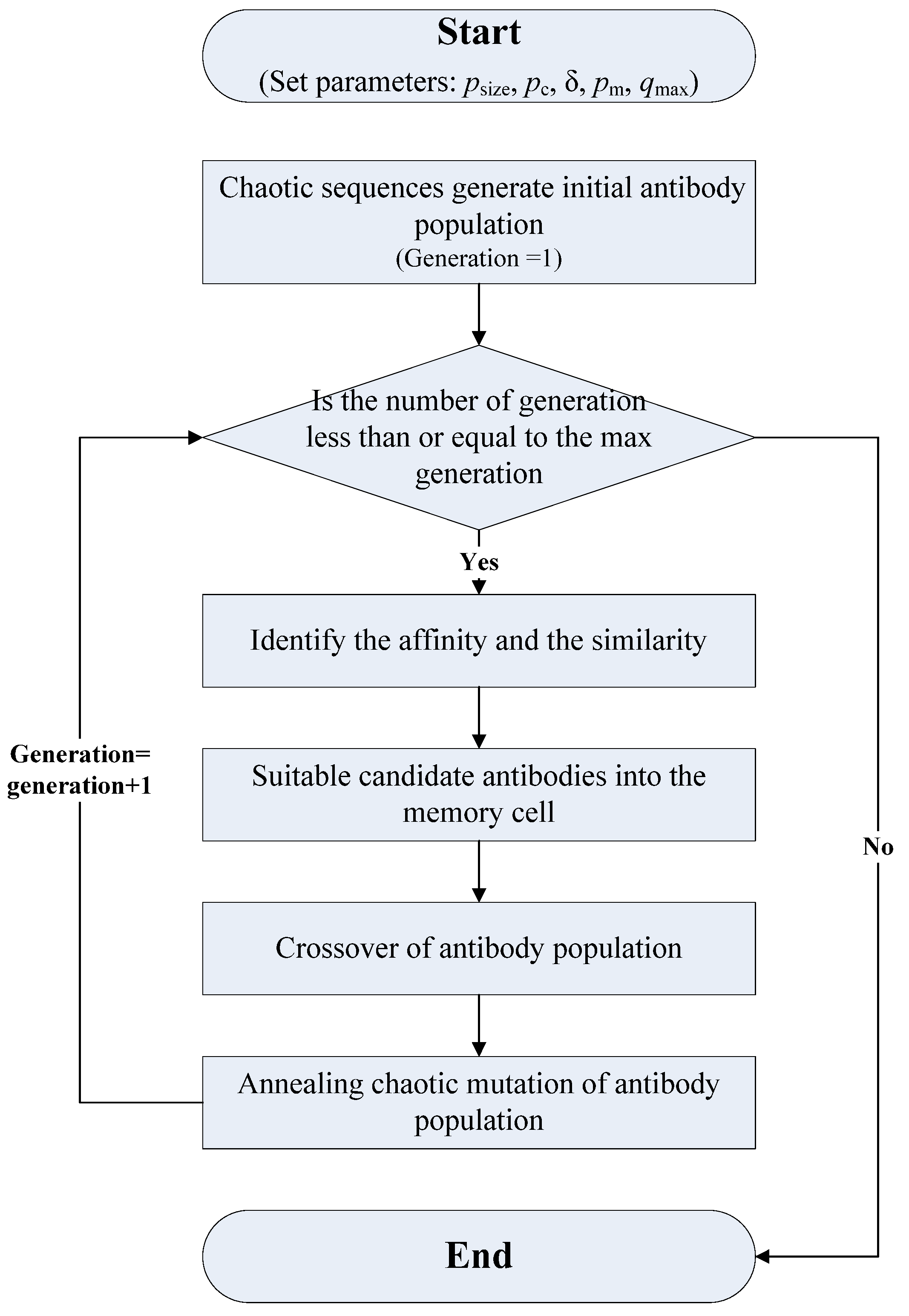
2.2. Chaotic Immune Algorithm (CIA) in Selecting Parameters of the SVR Model

The selection of the three parameters, σ, ε and C, of a SVR model influence the forecasting accuracy. However, structural methods for confirming efficient selection of parameters efficiently are lacking. Recently, Hong [38] applied an immune algorithm (IA) to determine the parameters of a SVR model, and found that the proposed model is superior to other competitive forecasting models (ANN and regression models). However, based on the IA operation procedure, if the population diversity of an initial population cannot be maintained under selective pressure, i.e., the initial individuals are not necessarily fully diversified in the search space, then an IA could only seek for the solutions in the narrow space and the solution is far from the global optimum (premature convergence). To overcome thise shortcoming, it is necessary to find some effective approach and improve the design or procedures of the IA to track in the solution space effectively and efficiently. One feasible approach is focused on the chaos approach, due to its easy implementation and special ability to avoid being trapped in local optima [44]. The application of chaotic sequences can be a good alternative to diversify the initial definition domain in stochastic optimization procedures, i.e., small changes in the parameter settings or the initial values in the model. Due to the ergodicity property of chaotic sequences, it will lead to very different future solution-finding behaviors, thus, chaotic sequences can be used to enrich the search behavior and to avoid being trapped in a local optimum [55]. There are lots of applications in optimization problema using chaotic sequences [56,57,58,59,60]. Coelho and Mariani [61] recently apply a chaotic artificial immune network (chaotic opt-aiNET) to solve the economic dispatch problem (EDP), based on Zaslavsky’s map by its spread-spectrum characteristic and large Lyapunov exponent to successfully escape from local optimum and to converge to a stable equilibrium. Therefore, it is believable that applying chaotic sequences to diversify the initial definition domain in IA’s initialization procedure (CIA) is a feasible approach to optimize the parameter selection in a SVR model. Recently, Wang et al. [62] also employed similar applications of CIA to determine the three parameters of a SVR model and obtained good performance in jumping out of the local optimum.

To design the CIA, many principal factors like identifying the affinity, selection of antibodies, crossover and mutation of antibody population are similar to the IA factors, and more procedural details about the CIA used in this study are as follows, and the corresponding flowchart is shown in Figure 1.

Figure 1. Chaotic immune algorithm (CIA) flowchart.

Figure 1. Chaotic immune algorithm (CIA) flowchart.

Step 1. Initialization of Antibody Population. The values of the three parameters in a SVR model in the ith iteration can be represented as $X_k^{(i)},k=C,\sigma \text{, }\epsilon$. Set $i=0$, and we employ Equation 7 to map the three parameters among the intervals (Min_k,Max_k) into chaotic variable $x_k^{(i)}$ located in the interval (0,1).

$$x_k^{(i)}=\frac{X_k^{(i)}-Mi{n}_k}{Ma{x}_k-Mi{n}_k},k=C\text{, }\sigma \text{, }\epsilon$$

(7)

Then, employing the chaotic sequence, defined as Equation 8 with $\mu =4$ to compute the next iteration chaotic variable, $x_k^{(i+1)}$:

$$\begin{gathered} x^{(i+1)}=\mu x^{(i)}(1-x^{(i)}) \\ {x}^{(i)}\in (0,1),i=0,1,2,\mathrm{...} \end{gathered}$$

(8)

where $x^{(i)}$ is the value of the chaotic variable x at the ith iteration; μ is the so-called bifurcation parameter of the system, $\mu \in [0,4]$. The system behavior varies significantly with μ, the value of μ determines whether $x^{(i)}$ stabilizes at a constant size, wags between a limited sequences of sizes, or whether $x^{(i)}$ behaves chaotically in an unpredictable pattern. For certain values of the parameter μ, of which μ = 4 is one, $x^{(i)}\in (0,1)$, but $x^{(i)}\notin \left\{0.25,\text{ 0.5, 0.75}\right\}$, and $x^{(i)}$ is distributed in the range (0,1), the above system exhibits chaotic behavior. We transform $x_k^{(i+1)}$ to obtain three parameters for the next iteration, $X_k^{(i+1)}$ with Equation 9:

$$X_k^{(i+1)}=Mi{n}_k+x_k^{(i+1)}(Ma{x}_k-Mi{n}_k)$$

(9)

After this transformation, the three parameters, C, σ, and ε, constitute the initial antibody population, and then will be represented by a binary-code string. For example, assume that an antibody contains 12 binary codes to represent three SVR parameters. Each parameter is thus expressed by four binary codes. Assume the set-boundaries for parameters σ, C, and ε are 2, 10, and 0.5 respectively, then, the antibody with binary-code “1 0 0 1 0 1 0 1 0 0 1 1” implies that the real values of the three parameters σ, C, and ε are 1.125, 3.125, and 0.09375, respectively. The number of initial antibodies is the same as the size of the memory cell. The size of the memory cell is set to 10 in this study.

Step 2. Identify the Affinity and the Similarity. A higher affinity value implies that an antibody has a higher activation with an antigen. To continue keeping the diversity of the antibodies stored in the memory cells, the antibodies with lower similarity have higher probability of being included in the memory cell. Therefore, an antibody with a higher affinity value and a lower similarity value has a good likelihood of entering the memory cells. The affinity between the antibody and antigen is defined as Equation 10:

$$A{g}_k=1/(1+d_k)$$

(10)

where d_k denotes the SVR forecasting errors obtained by the antibody k. The similarity between antibodies is expressed as in Equation 11:

$$A{b}_{ij}=1/(1+T_{ij})$$

(11)

where T_ij denotes the difference between the two SVR forecasting errors obtained by the antibodies inside (existed) and outside (will be entering) the memory cell.

Step 3. Selection of Antibodies in the Memory Cell. Antibodies with higher values of Ag_k are considered to be potential candidates for entering the memory cell. However, the potential antibody candidates with Ab_ij values exceeding a certain threshold are not qualified to enter the memory cell. In this investigation, the threshold value is set to 0.9.

Step 4. Crossover of Antibody Population. New antibodies are created via crossover and mutation operations. To perform crossover operation, strings representing antibodies are paired randomly. Moreover, the proposed scheme adopts the single-point-crossover principle. Segments of paired strings (antibodies) between two determined break-points are swapped. In this investigation, the probability of crossover (p_c) is set as 0.5. Finally, the three crossover parameters are decoded into a decimal format.

Step 5. Annealing Chaotic Mutation of Antibody Population. For the ith iteration (generation) crossover antibody population (${\widehat{X}}_k^{(i)},k=C,\sigma \text{, }\epsilon$) of current solution space (Min_k,Max_k) are mapped to chaotic variable interval [0,1] to form the crossover chaotic variable space ${\widehat{x}}_k^{(i)},k=C,\sigma \text{, }\epsilon$, as Equation 12:

$${\widehat{x}}_k^{(i)}=\frac{{\widehat{X}}_k^{(i)}-Mi{n}_k}{Ma{x}_k-Mi{n}_k},k=\text{C, }\sigma \text{, }\epsilon \text{, }i=1,\text{ 2},\mathrm{......}\text{,}{q}_{\max }$$

(12)

where q_max is the maximum evolutional generation of the population. Then, the ith chaotic variable $x_k^{(i)}$ is summed up to ${\widehat{x}}_k^{(i)}$ and the chaotic mutation variable are also mapped to interval [0,1] as in Equation 13:

$${\tilde{x}}_k^{(i)}={\widehat{x}}_k^{(i)}+\delta x_k^{(i)}$$

(13)

where δ is the annealing operation. Finally, the chaotic mutation variable obtained in interval [0,1] is mapped to the solution interval (Min_k,Max_k) by definite probability of mutation (p_m), thus completing a mutative operation:

$${\tilde{X}}_k^{(i)}=Mi{n}_k+{\tilde{x}}_k^{(i)}\left(Ma{x}_k-Mi{n}_k\right)$$

(14)

Step 6. Stopping Criteria. If the number of generations equals a given scale, then the best antibody is a solution, otherwise return to Step 2. The CIA is used to seek a better combination of the three parameters in the SVR. The value of the mean absolute percentage error (MAPE) is used as the criterion (the smallest value of MAPE) of forecasting errors to determine the suitable parameters used in SVR model in this investigation, which is given by Equation 15:

$$\text{MAPE}=\frac{1}{N}{\displaystyle \sum _{i=1}^N\left|\frac{f_i-{\widehat{f}}_i}{f_i}\right|}\times 100\%$$

(15)

where N is the number of forecasting periods; ƒ_i is the actual value at period i; ${\widehat{f}}_i$ denotes is the forecasting value at period i.

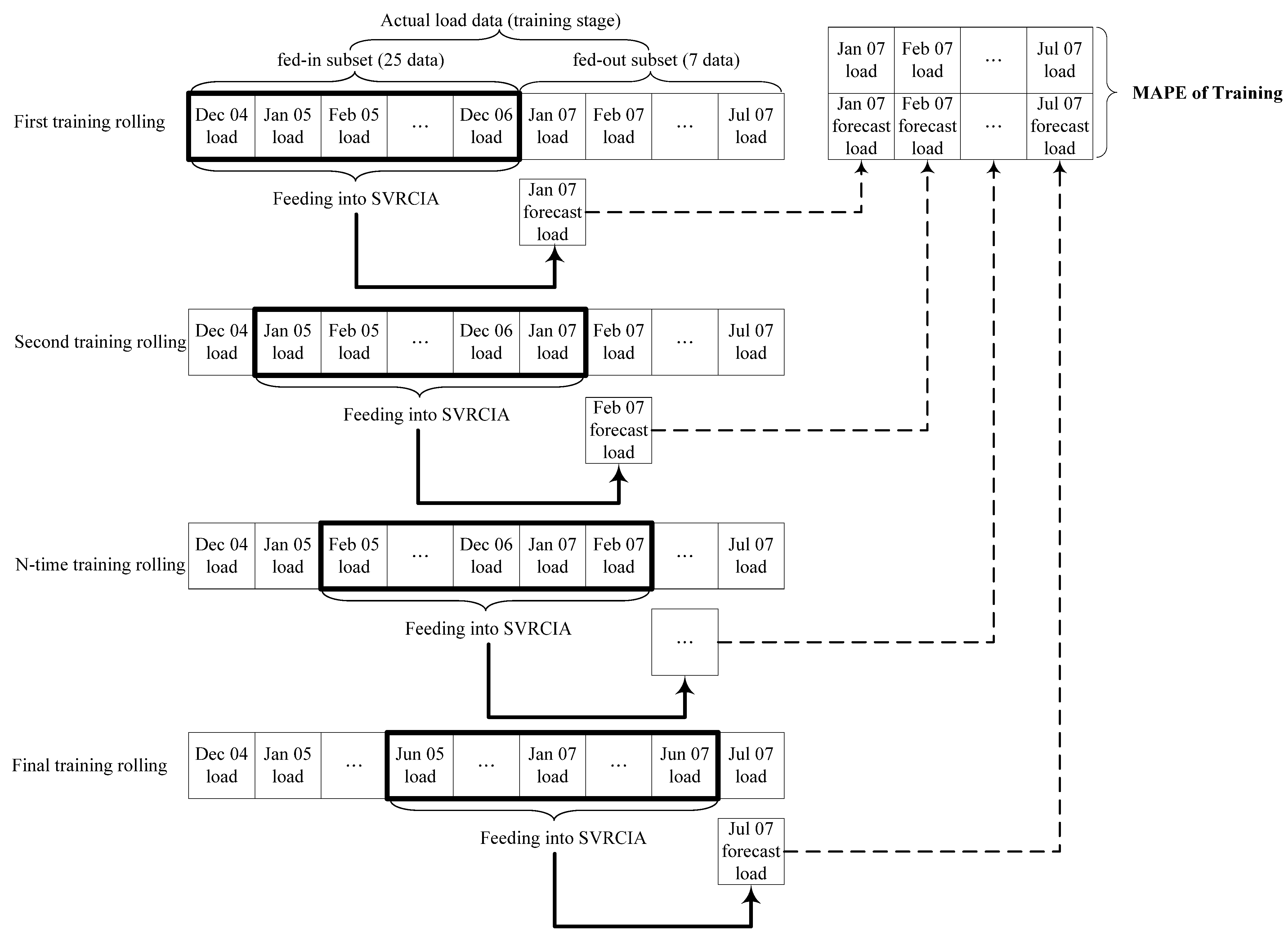
2.3. Seasonal Adjustment

Due to the difference in demand from month to month and season to season, electric energy demands also demonstrate a cyclic (seasonal) tendency, so any model attempting to accomplish the goal of high accurate forecasting performance, must estimate this seasonal component. There are several approaches to estimate the seasonal index of data series [50,63,64], including product-model type and non-product-model type. Based on the data series type consideration, this investigation employed Deo and Hurvich’s [63] approach to compute the seasonal index, as shown in Equation 16:

$$pea{k}_t=\frac{a_t}{f_t}=\frac{a_t}{{\displaystyle \sum _{i=1}^N\left({\beta }_i^{*}-{\beta }_i\right)K(x_i,x)}+b}$$

(16)

where t = j, l + j, 2l + j,…,(m − 1)l + j only for the same time point (month) in each period. Then, the seasonal index (SI) for each time point (month) j is computed as Equation 17:

$$S{I}_j=\frac{1}{m}\left(pea{k}_j+pea{k}_{l+j}+\cdots +pea{k}_{(m-1)l+j}\right)$$

(17)

where j = 1,2,…,l. Eventually, the forecasting value of the SSVRCIA is obtained by Equation 18:

$$f_{N+k}=\left({\displaystyle \sum _{i=1}^N\left({\beta }_i^{*}-{\beta }_i\right)K(x_i,x_{N+k})}+b\right)\times S{I}_k$$

(18)

where k = 1,2,…,l implies the time point (month) in another period (for forecasting period).

Table 1. Monthly electric load in Northeastern China (from January 2004 to April 2009). Units: hundred million kW/h.

Time	Electric Load	Time	Electric Load	Time	Electric Load
January 2004	129.08	November 2005	150.84	September 2007	175.41
February 2004	127.24	December 2005	165.27	October 2007	179.64
March 2004	136.95	January 2006	155.31	November 2007	188.89
April 2004	125.34	February 2006	138.5	December 2007	197.62
May 2004	126.86	March 2006	133.27	January 2008	200.35
June 2004	129.34	April 2006	151.41	February 2008	169.24
July 2004	131.91	May 2006	155.63	March 2008	196.97
August 2004	136.22	June 2006	155.7	April 2008	186.15
September 2004	131.56	July 2006	162.98	May 2008	188.485
October 2004	134.62	August 2006	163.41	June 2008	190.82
November 2004	144.62	September 2006	157.57	July 2008	196.53
December 2004	154.62	October 2006	160.15	August 2008	197.67
January 2005	151.48	November 2006	168.13	September 2008	183.77
February 2005	126.74	December 2006	180.71	October 2008	181.07
March 2005	148.57	January 2007	179.94	November 2008	180.56
April 2005	136.6	February 2007	147.29	December 2008	189.03
May 2005	138.83	March 2007	172.45	January 2009	182.07
June 2005	136.6	April 2007	169.98	February 2009	167.35
July 2005	146.21	May 2007	173.21	March 2009	189.3
August 2005	146.09	June 2007	177.43	April 2009	175.84
September 2005	140.04	July 2007	184.29
October 2005	142.02	August 2007	183.53

Table 1. Monthly electric load in Northeastern China (from January 2004 to April 2009). Units: hundred million kW/h.

Time	Electric Load	Time	Electric Load	Time	Electric Load
January 2004	129.08	November 2005	150.84	September 2007	175.41
February 2004	127.24	December 2005	165.27	October 2007	179.64
March 2004	136.95	January 2006	155.31	November 2007	188.89
April 2004	125.34	February 2006	138.5	December 2007	197.62
May 2004	126.86	March 2006	133.27	January 2008	200.35
June 2004	129.34	April 2006	151.41	February 2008	169.24
July 2004	131.91	May 2006	155.63	March 2008	196.97
August 2004	136.22	June 2006	155.7	April 2008	186.15
September 2004	131.56	July 2006	162.98	May 2008	188.485
October 2004	134.62	August 2006	163.41	June 2008	190.82
November 2004	144.62	September 2006	157.57	July 2008	196.53
December 2004	154.62	October 2006	160.15	August 2008	197.67
January 2005	151.48	November 2006	168.13	September 2008	183.77
February 2005	126.74	December 2006	180.71	October 2008	181.07
March 2005	148.57	January 2007	179.94	November 2008	180.56
April 2005	136.6	February 2007	147.29	December 2008	189.03
May 2005	138.83	March 2007	172.45	January 2009	182.07
June 2005	136.6	April 2007	169.98	February 2009	167.35
July 2005	146.21	May 2007	173.21	March 2009	189.3
August 2005	146.09	June 2007	177.43	April 2009	175.84
September 2005	140.04	July 2007	184.29
October 2005	142.02	August 2007	183.53

3. A Numerical Results

3.1. Data Set

To based our comparisons on the same conditions, this study uses historical monthly electric load data from Northeast China to compare the forecasting performance of the proposed SSVRCIA model with those of ARIMA and TF-ε-SVR-SA models proposed by Wang et al. [50]. In addition, due to verification of performance of seasonal adjustment mechanism, the SVRCIA model (without seasonal adjustment mechanism) is also implemented for comparison. Table 1 lists the data used in this example. Totally, there are 64 data points (from January 2004 to April 2009) of Northeastern China’s monthly electric load. However, based on Wang et al. [50]’s support vectors computation, only 53 months’ of data (from December 2004 to April 2009) are suggested. Thus, the employed data are divided into three data sets, the training data set (32 months, December 2004 to July 2007), validation data set (14 months, August 2007 to September 2008), and, to ensure the same comparison conditions, the testing data set (7 months, from October 2008 to April 2009), is shown in Table 2.

Table 2. Training, validation, and testing data sets of the proposed model.

Data Sets	SVRCIA and SSVRCIA Models	TF-ε-SVR-SA Model (Wang et al., 2009)
Training data	December 2004–July 2007	December 2004–September 2008
Validation data	August 2007–September 2008
Testing data	October 2008–April 2009	October 2008–April 2009

Table 2. Training, validation, and testing data sets of the proposed model.

Data Sets	SVRCIA and SSVRCIA Models	TF-ε-SVR-SA Model (Wang et al., 2009)
Training data	December 2004–July 2007	December 2004–September 2008
Validation data	August 2007–September 2008
Testing data	October 2008–April 2009	October 2008–April 2009

Figure 2. The rolling-base forecasting procedure (training stage).

Figure 2. The rolling-base forecasting procedure (training stage).

3.2. SSVRCIA Electric Load Forecasting Model

Before conducting the seasonal adjustment for the SSVRCIA model, it is necessary to implement the CIA algorithm to determine suitable values of the three parameters in a SVR model. The parameters of the CIA in the proposed model are experimentally set as shown in Table 3. For the SVRCIA modeling procedure, in the training stage, a rolling-based forecasting procedure (Figure 2), which divides the training data into two subsets, namely the fed-in subset (for example, 25 load data points) and the fed-out subset (7 load data points), respectively. First, the primary 25 load data of the fed-in subset are fed into the proposed model, the structural risk minimization principle is employed to minimize the training error, then, we obtain the one-step ahead forecasting load, namely the 26th forecasting load. Second, the next 25 load data points, including 24 of the fed-in subset data (from 2nd to 25th) pulsing the 26th data in the fed-out subset, are similarly fed again into the proposed model, the structural risk minimization principle is also employed to minimize the training error, then, we obtain the one-step ahead forecasting load, namely the 27th forecasting load. The rolling-based forecasting procedure is repeated till the 32nd forecasting load is obtained. Meanwhile, the training error in this training stage is also obtained. In the validation and testing stage, a one-hour-ahead forecasting policy is adopted. Then, several types of data-rolling are considered to forecast the electric load in the next point (month). Different values of the electric load in a time series are fed into the SVRCIA model to forecast the electric load in the next validation period. While training errors improvement occurs, the three kernel parameters, σ, C, and ε of the SVRCIA model adjusted by the CIA algorithm are employed to calculate the validation error. Then, the adjusted parameters with minimum validation error are selected as the most appropriate parameters. Table 4 indicates that SVRCIA models perform the best when 25 input data are used for electric load forecasting.

Table 3. CIA’s parameters setting.

Population Size (${\mathit{p}}_{\mathit{s}\mathit{i}\mathit{z}\mathit{e}}$)	Maximal Generation (${\mathit{q}}_{\mathbf{max}}$)	Probability of Crossover (${\mathit{p}}_{\mathit{c}}$)	The Annealing Operation Parameter ($\mathit{\delta }$)	Probability of Mutation (${\mathit{p}}_{\mathit{m}}$)
200	500	0.5	0.9	0.1

Table 3. CIA’s parameters setting.

Population Size (${\mathit{p}}_{\mathit{s}\mathit{i}\mathit{z}\mathit{e}}$)	Maximal Generation (${\mathit{q}}_{\mathbf{max}}$)	Probability of Crossover (${\mathit{p}}_{\mathit{c}}$)	The Annealing Operation Parameter ($\mathit{\delta }$)	Probability of Mutation (${\mathit{p}}_{\mathit{m}}$)
200	500	0.5	0.9	0.1

Table 4. Forecasting results and associated parameters of the SVRCIA model.

Nos. of Input Data	Parameters			MAPE of Testing (%)
	σ	C	ε
5	14.744	347.33	1.8570	4.1953
10	9.9515	90.244	0.1459	3.638
15	109.06	7298.3	11.953	3.897
20	48.030	8399.7	14.372	3.514
25	30.262	4767.3	22.114	3.0411

Table 4. Forecasting results and associated parameters of the SVRCIA model.

Nos. of Input Data	Parameters			MAPE of Testing (%)
	σ	C	ε
5	14.744	347.33	1.8570	4.1953
10	9.9515	90.244	0.1459	3.638
15	109.06	7298.3	11.953	3.897
20	48.030	8399.7	14.372	3.514
25	30.262	4767.3	22.114	3.0411

Now the seasonal term is considered. For the monthly electric load in Northeastern China, each month has a different electric demand pattern, the seasonal length is verified as 12 [50], thus, there are 12 points (months) in each electric load cyclic year. The seasonal indexes for each point (month) are calculated based on the 46 forecasting values of the SVRCIA model both in training (32 forecasting values) and validation (14 forecasting values) stages, as shown in Table 5. Those indices with values smaller than 1 imply that the average forecasts (based on 32 training forecasts and 14 validation forecasts) of the SVRCIA model are overestimated, i.e., the smaller a seasonal index is, the higher the overestimation of electric load is. Thus, overproduced supplies would lead to energy losses. On the contrary, the higher the seasonal index is, the lower the underestimation of electric load is, i.e., the months with a higher seasonal index (larger than 1) may be potential months with limited amounts of useable electric load in the future.

Table 5. The seasonal indexes for each time point (month).

Time Point (Month)	Seasonal Index	Time Point (Month)	Seasonal Index
January	1.0153	July	1.0663
February	0.9089	August	1.0615
March	1.0126	September	1.0076
April	0.9853	October	0.9734
May	1.0187	November	1.0247
June	1.0225	December	1.0614

Table 5. The seasonal indexes for each time point (month).

Time Point (Month)	Seasonal Index	Time Point (Month)	Seasonal Index
January	1.0153	July	1.0663
February	0.9089	August	1.0615
March	1.0126	September	1.0076
April	0.9853	October	0.9734
May	1.0187	November	1.0247
June	1.0225	December	1.0614

Table 6. Forecasting results of the ARIMA, TF-ε-SVR-SA, SVRCIA, and SSVRCIA models (units: hundred million kW/h).

Time Point (Month)	Actual	ARIMA(1,1,1)	TF-ε-SVR-SA	SVRCIA	SSVRCIA
October 2008	181.07	192.9316	184.5035	179.0276	174.2737
November 2008	180.56	191.127	190.3608	179.4118	183.8444
December 2008	189.03	189.9155	202.9795	179.7946	190.8367
January 2009	182.07	191.9947	195.7532	180.1759	182.9343
February 2009	167.35	189.9398	167.5795	180.5557	164.1062
March 2009	189.30	183.9876	185.9358	180.9341	183.2106
April 2009	175.84	189.3480	180.1648	178.1036	175.4833
MAPE (%)		6.044	3.799	3.041	1.766

Table 6. Forecasting results of the ARIMA, TF-ε-SVR-SA, SVRCIA, and SSVRCIA models (units: hundred million kW/h).

Time Point (Month)	Actual	ARIMA(1,1,1)	TF-ε-SVR-SA	SVRCIA	SSVRCIA
October 2008	181.07	192.9316	184.5035	179.0276	174.2737
November 2008	180.56	191.127	190.3608	179.4118	183.8444
December 2008	189.03	189.9155	202.9795	179.7946	190.8367
January 2009	182.07	191.9947	195.7532	180.1759	182.9343
February 2009	167.35	189.9398	167.5795	180.5557	164.1062
March 2009	189.30	183.9876	185.9358	180.9341	183.2106
April 2009	175.84	189.3480	180.1648	178.1036	175.4833
MAPE (%)		6.044	3.799	3.041	1.766

Table 6 shows the actual values and the forecast values obtained using various forecasting models: ARIMA(1,1,1), TF-ε-SVR-SA, SVRCIA, and SSVRCIA. The MAPE values are calculated to compare fairly the proposed models with other alternative models. The proposed SSVRCIA model has smaller MAPE values than the ARIMA, TF-ε-SVR-SA, and SVRCIA models for capturing electric load cyclic trends on monthly average basis. Furthermore, to verify the significance of accuracy improvement of SSVRCIA model comparing with ARIMA(1,1,1), TF-ε-SVR-SA, and SVRCIA models, a statistical test, namely the Wilcoxon signed-rank test, is conducted at the 0.025 and 0.05 significance levels in one-tail-tests (Table 7).

Table 7. Wilcoxon signed-rank test.

Compared Models	Wilcoxon Signed-Rank Test
	α = 0.025 W = 2	α = 0.05 W = 3
SSVRCIA vs. ARIMA(1,1,1)	1 *	1 *
SSVRCIA vs. TF-ε-SVR-SA	0 *	0 *
SSVRCIA vs. SVRCIA	2 *	2 *

* denote that SSVRCIA model significantly outperforms other alternative models.

Table 7. Wilcoxon signed-rank test.

Compared Models	Wilcoxon Signed-Rank Test
	α = 0.025 W = 2	α = 0.05 W = 3
SSVRCIA vs. ARIMA(1,1,1)	1 *	1 *
SSVRCIA vs. TF-ε-SVR-SA	0 *	0 *
SSVRCIA vs. SVRCIA	2 *	2 *

* denote that SSVRCIA model significantly outperforms other alternative models.

From Table 7, it is seen that the SSVRCIA model outperforms the ARIMA(1,1,1) model significantly, due to its theoretical assumption of a convex set. In addition, the SSVRCIA model is also significantly superior to the TF-ε-SVR-SA model, not only because of the superior searching capability of CIA to determine proper parameters in a SVR model, but also because of the use of a seasonal adjustment mechanism to adjust the seasonal/cyclic effects of electric loads. Finally, the SSVRCIA model also significantly outperforms the SVRCIA model, obviously, the seasonal adjustment mechanism employed here is proficient in dealing with such cyclic data types.

4. Conclusions

From the historical data, the electric load values in Northern China show not only a strong growth trend but also an obvious monthly seasonal/cyclic tendency. This is a common electric load phenomenon in developing countries. However, the role of electric demand growth rate forecasting seems to be to avoid overproduction or underproduction of electric loads. This study introduces the application of a forecasting technique, SSVRCIA, to investigate its feasibility for forecasting electric loads. The experimental results indicate that the SSVRCIA model has better forecasting performance than the ARIMA(1,1,1), TF-ε-SVR-SA, and SVRCIA models. The superior performance of the SSVRCIA model is not only because of its theoretical assumptions of a convex set while SVR modeling, but also because of the superior searching capability of CIA to determine the proper parameters in SVR (this is why it outperforms the TF-ε-SVR-SA model) and effective seasonal adjustment mechanism (this is why it outperforms the SVRCIA model). By contrast, ARIMA model employs the parametric technique which is based on specific assumptions, such as linear relationships between the current value of the underlying variables and previous values of the variable and error terms, and these assumptions are not completely in line with real world problems.

This investigation is the first to apply the SVR with CIA and seasonal adjustment for forecasting monthly electric loads. Many forecasting methodologies have been proposed to deal with the seasonality of electric loads, but most models are time consuming in verifying the suitable time-phase divisions, particularly when the sample size is large. In this investigation, the SSVRCIA model provides a convenient and valid alternative for electric load forecasting. The SSVRCIA model directly uses historical monthly electric data and then determines suitable parameters by efficient optimization algorithms. In addition, the proposed SSVRCIA model is also a hybrid forecasting models; some other advanced optimization algorithms for parameters selection can be further applied for the SVR model.

References

1. Fan, S.; Chen, L. Short-term load forecasting based on an adaptive hybrid method. IEEE Trans. Power Syst. 2006, 21, 392–401. [Google Scholar] [CrossRef]
2. Morimoto, R.; Hope, C. The impact of electricity supply on economic growth in Sri Lanka. Energy Econ. 2004, 26, 77–85. [Google Scholar] [CrossRef]
3. Box, G.E.P.; Jenkins, G.M. Time Series Analysis, Forecasting and Control; Holden-Day Press: San Francisco, CA, USA, 1970. [Google Scholar]
4. Chen, J.F.; Wang, W.M.; Huang, C.M. Analysis of an adaptive time-series autoregressive moving-average (ARMA) model for short-term load forecasting. Electr. Power Syst. Res. 1995, 34, 187–196. [Google Scholar] [CrossRef]
5. Vemuri, S.; Hill, D.; Balasubramanian, R. Load forecasting using stochastic models. In Proceedings of the 8th Power Industrial Computing Application Conference, Minneapolis, MN, USA, 1973; pp. 31–37.
6. Christianse, W.R. Short term load forecasting using general exponential smoothing. IEEE Trans. Power Apparatus Syst. 1971, 90, 900–911. [Google Scholar] [CrossRef]
7. Park, J.H.; Park, Y.M.; Lee, K.Y. Composite modeling for adaptive short-term load forecasting. IEEE Trans. Power Syst. 1991, 6, 450–457. [Google Scholar] [CrossRef]
8. Brown, R.G. Introduction to Random Signal Analysis and Kalman Filtering; John Wiley & Sons Inc. Press: New York, NY, USA, 1983. [Google Scholar]
9. Gelb, A. Applied Optimal Estimation; The MIT Press: Cambridge, MA, USA, 1974. [Google Scholar]
10. Moghram, I.; Rahman, S. Analysis and evaluation of five short-term load forecasting techniques. IEEE Trans. Power Syst. 1989, 4, 1484–1491. [Google Scholar] [CrossRef]
11. Asbury, C. Weather load model for electric demand energy forecasting. IEEE Trans. Power Apparatus Syst. 1975, 94, 1111–1116. [Google Scholar] [CrossRef]
12. Papalexopoulos, A.D.; Hesterberg, T.C. A regression-based approach to short-term system load forecasting. IEEE Trans. Power Syst. 1990, 5, 1535–1547. [Google Scholar] [CrossRef]
13. Soliman, S.A.; Persaud, S.; El-Nagar, K.; El-Hawary, M.E. Application of least absolute value parameter estimation based on linear programming to short-term load forecasting. Int. J. Electr. Power Energy Syst. 1997, 19, 209–216. [Google Scholar] [CrossRef]
14. Rahman, S.; Bhatnagar, R. An expert system based algorithm for short-term load forecasting. IEEE Trans. Power Syst. 1998, 3, 392–399. [Google Scholar] [CrossRef]
15. Chiu, C.C.; Kao, L.J.; Cook, D.F. Combining a Neural Network with a rule-based expert system approach for short-term power load forecasting in Taiwan. Expert Syst. Appl. 1997, 13, 299–305. [Google Scholar] [CrossRef]
16. Rahman, S.; Hazim, O. A generalized knowledge-based short-term load- forecasting technique. IEEE Trans. Power Syst. 1993, 8, 508–514. [Google Scholar] [CrossRef]
17. Park, D.C.; El-Sharkawi, M.A.; Marks, R.J., II; Atlas, L.E.; Damborg, M.J. Electric load forecasting using an artificial neural network. IEEE Trans. Power Syst. 1991, 6, 442–449. [Google Scholar] [CrossRef]
18. Novak, B. Superfast autoconfiguring artificial neural networks and their application to power systems. Electr. Power Syst. Res. 1995, 35, 11–16. [Google Scholar] [CrossRef]
19. Darbellay, G.A.; Slama, M. Forecasting the short-term demand for electricity—do neural networks stand a better chance? Int. J. Forecast. 2000, 16, 71–83. [Google Scholar] [CrossRef]
20. Abdel-Aal, R.E. Short-term hourly load forecasting using abductive networks. IEEE Trans. Power Syst. 2004, 19, 164–173. [Google Scholar] [CrossRef]
21. Hsu, C.C.; Chen, C.Y. Regional load forecasting in Taiwan—application of artificial neural networks. Energy Convers. Manag. 2003, 44, 1941–1949. [Google Scholar] [CrossRef]
22. Suykens, J.A.K. Nonlinear modelling and support vector machines. In Proceedings of IEEE Instrumentation and Measurement Technology Conference, Budapest, Hungary, 2001; pp. 287–294.
23. Tay, F.E.H.; Cao, L.J. Application of support vector machines in financial time series forecasting. Omega 2001, 29, 309–317. [Google Scholar] [CrossRef]
24. Huang, W.; Nakamori, Y.; Wang, S.Y. Forecasting stock market movement direction with support vector machine. Comput. Oper. Res. 2005, 32, 2513–2522. [Google Scholar] [CrossRef]
25. Hung, W.M.; Hong, W.C. Application of SVR with improved ant colony optimization algorithms in exchange rate forecasting. Control Cybern. 2009, 38, 863–891. [Google Scholar]
26. Pai, P.F.; Lin, C.S. A hybrid ARIMA and support vector machines model in stock price forecasting. Omega 2005, 33, 497–505. [Google Scholar] [CrossRef]
27. Pai, P.F.; Lin, C.S.; Hong, W.C.; Chen, C.T. A hybrid support vector machine regression for exchange rate prediction. Int. J. Inf. Manag. Sci. 2006, 17, 19–32. [Google Scholar]
28. Hong, W.C.; Dong, Y.; Chen, L.Y.; Wei, S.Y. SVR with hybrid chaotic genetic algorithms for tourism demand forecasting. Appl. Soft Comput. 2011, 11, 1881–1890. [Google Scholar] [CrossRef]
29. Pai, P.F.; Hong, W.C. An improved neural network model in forecasting arrivals. Ann. Tourism Res. 2005, 32, 1138–1141. [Google Scholar] [CrossRef]
30. Pai, P.F.; Hong, W.C. Software reliability forecasting by support vector machines with simulated annealing algorithms. J. Syst. Softw. 2006, 79, 747–755. [Google Scholar] [CrossRef]
31. Hong, W.C.; Pai, P.F. Predicting engine reliability by support vector machines. Int. J. Adv. Manuf. Technol. 2006, 28, 154–161. [Google Scholar] [CrossRef]
32. Hong, W.C. Rainfall forecasting by technological machine learning models. Appl. Math. Comput. 2008, 200, 41–57. [Google Scholar] [CrossRef]
33. Hong, W.C.; Pai, P.F. Potential assessment of the support vector regression technique in rainfall forecasting. Water Resour. Manag. 2007, 21, 495–513. [Google Scholar] [CrossRef]
34. Wang, W.; Xu, Z.; Lu, J.W. Three improved neural network models for air quality forecasting. Eng. Comput. 2003, 20, 192–210. [Google Scholar] [CrossRef]
35. Mohandes, M.A.; Halawani, T.O.; Rehman, S.; Hussain, A.A. Support vector machines for wind speed prediction. Renew Energy 2004, 29, 939–947. [Google Scholar] [CrossRef]
36. Hong, W.C. Hybrid evolutionary algorithms in a SVR-based electric load forecasting model. Int. J. Electr. Power Energy Syst. 2009, 31, 409–417. [Google Scholar] [CrossRef]
37. Hong, W.C. Chaotic particle swarm optimization algorithm in a support vector regression electric load forecasting model. Energy Convers. Manag. 2009, 50, 105–117. [Google Scholar] [CrossRef]
38. Hong, W.C. Electric load forecasting by support vector model. Appl. Math. Modell. 2009, 33, 2444–2454. [Google Scholar] [CrossRef]
39. Pai, P.F.; Hong, W.C. Support vector machines with simulated annealing algorithms in electricity load forecasting. Energy Convers. Manag. 2005, 46, 2669–2688. [Google Scholar] [CrossRef]
40. Pai, P.F.; Hong, W.C. Forecasting regional electric load based on recurrent support vector machines with genetic algorithms. Electr. Power Syst. Res. 2005, 74, 417–425. [Google Scholar] [CrossRef]
41. Hong, W.C. Application of chaotic ant swarm optimization in electric load forecasting. Energy Policy 2010, 38, 5830–5839. [Google Scholar] [CrossRef]
42. Mori, K.; Tsukiyama, M.; Fukuda, T. Immune algorithm with searching diversity and its application to resource allocation problem. Trans. Inst. Electr. Eng. Jpn. 1993, 113-C, 872–878. [Google Scholar]
43. Prakash, A.; Khilwani, N.; Tiwari, M.K.; Cohen, Y. Modified immune algorithm for job selection and operation allocation problem in flexible manufacturing system. Adv. Eng. Softw. 2008, 39, 219–232. [Google Scholar] [CrossRef]
44. Wang, L.; Zheng, D.Z.; Lin, Q.S. Survey on chaotic optimization methods. Comput. Technol. Autom. 2001, 20, 1–5. [Google Scholar]
45. Li, B.; Jiang, W. Optimizing complex functions by chaos search. Cybern. Syst. 1998, 29, 409–419. [Google Scholar] [CrossRef]
46. Ohya, M. Complexities and their applications to characterization of chaos. Int. J. Theor. Phys. 1998, 37, 495–505. [Google Scholar] [CrossRef]
47. Lorenz, E.N. Deterministic nonperiodic flow. J. Atmos. Sci. 1963, 20, 130–141. [Google Scholar] [CrossRef]
48. Dagum, E.B. Modelling, forecasting and seasonally adjusting economic time series with the X-11 ARIMA method. J. R. Stat. Soc. Series D 1978, 27, 203–216. [Google Scholar]
49. Kenny, P.B.; Durbin, J. Local trend estimation and seasonal adjustment of economic and social time series. J. R. Stat. Soc. Series A 1982, 145, 1–41. [Google Scholar] [CrossRef]
50. Wang, J.; Zhu, W.; Zhang, W.; Sun, D. A trend fixed on firstly and seasonal adjustment model combined with the ε-SVR for short-term forecasting of electricity demand. Energy Policy 2009, 37, 4901–4909. [Google Scholar] [CrossRef]
51. Xiao, Z.; Ye, S.J.; Zhong, B.; Sun, C.X. BP neural network with rough set for short term load forecasting. Expert Syst. Appl. 2009, 36, 273–279. [Google Scholar] [CrossRef]
52. Vapnik, V. The Nature of Statistical Learning Theory; Springer-Verlag Press: New York, NY, USA, 1995. [Google Scholar]
53. Amari, S.; Wu, S. Improving support vector machine classifiers by modifying kernel functions. Neural Netw. 1999, 12, 783–789. [Google Scholar] [CrossRef] [PubMed]
54. Vojislav, K. Learning and Soft Computing—Support Vector Machines, Neural Networks and Fuzzy Logic Models; The MIT Press: Cambridge, MT, USA, 2001. [Google Scholar]
55. Pan, H.; Wang, L.; Liu, B. Chaotic annealing with hypothesis test for function optimization in noisy environments. Chaos Solitons Fractals 2008, 35, 888–894. [Google Scholar] [CrossRef]
56. Zuo, X.Q.; Fan, Y.S. A chaos search immune algorithm with its application to neuro-fuzzy controller design. Chaos Solitons Fractals 2006, 30, 94–109. [Google Scholar] [CrossRef]
57. Liu, B.; Wang, L.; Jin, Y.H.; Tang, F.; Huang, D.X. Improved particle swam optimization combined with chaos. Chaos Solitons Fractals 2005, 25, 1261–1271. [Google Scholar] [CrossRef]
58. Yang, D.; Li, G.; Cheng, G. On the efficiency of chaos optimization algorithms for global optimization. Chaos Solitons Fractals 2007, 34, 1366–1375. [Google Scholar] [CrossRef]
59. Li, L.; Yang, Y.; Peng, H.; Wang, X. Parameters identification of chaotic systems via chaotic ant swarm. Chaos Solitons Fractals 2006, 28, 1204–1211. [Google Scholar] [CrossRef]
60. Tavazoei, M.S.; Haeri, M. Comparison of different one-dimensional maps as chaotic search pattern in chaos optimization algorithms. Appl. Math. Comput. 2007, 187, 1076–1085. [Google Scholar] [CrossRef]
61. Coelho, L.D.S.; Mariani, V.C. Chaotic artificial immune approach applied to economic dispatch of electric energy using thermal units. Chaos Solitons Fractals 2009, 40, 2376–2383. [Google Scholar] [CrossRef]
62. Wang, J.; Wang, Y.; Zhang, C.; Du, W.; Zhou, C.; Liang, Y. Parameter selection of support vector regression based on a novel chaotic immune algorithm. In Proceedings of the 4th International Conference on Innovative Computing, Information and Control, City, Country, 2009; pp. 652–655.
63. Deo, R.; Hurvich, C. Forecasting realized volatility using a long-memory stochastic volatility model: estimation, prediction and seasonal adjustment. J. Econometrics 2006, 131, 29–58. [Google Scholar] [CrossRef]
64. Azadeh, A.; Ghaderi, S.F. Annual electricity consumption forecasting by neural network in high energy consuming industrial sectors. Energy Convers. Manag. 2008, 49, 2272–2278. [Google Scholar] [CrossRef]