Petri Net Model and Reliability Evaluation for Wind Turbine Hydraulic Variable Pitch Systems

Abstract

Based on an analysis of the working principles of the hydraulic variable pitch system of a wind turbine, a novel Petri net model and reliability evaluation method are proposed. First, Petri net theory is adopted to build a model for each discrete state of the operation of the hydraulic pitch system of the wind turbine and at the same time a fault Petri net model is established. Then through qualitative analysis and quantitative calculations based on the fault Petri net, the system reliability indexes are obtained. During the qualitative analysis process, in order to more conveniently find the minimal cut sets of the fault Petri net, a Visual C++ 6.0-based algorithm is compiled and the minimal cut sets are tested correctly with another method. During the quantitative calculation process, the fault probability has been obtained from the equations according to the fault probability of libraries and transitions between different states. Not only does the proposed Petri net describe the structure, function and operation of the hydraulic pitch system with a graphic language, but the fault Petri net model can also clearly express the logical relations among faults. The novel Petri net model offers simple calculations and the prospect of broad applicability and the new reliability evaluation method provides an important reference for the performance evaluation of these systems.

1. Introduction

It is believed that in the near future wind energy will be one of the most cost effective sources of electrical power [1]. Nowadays, larger wind turbines, based on variable speed operation with pitch control, constitute the majority of the more widespread large wind turbines [2]. The use of variable-speed wind turbines has increased in recent years, not only due to their ability to better capture wind energy, compared to fixed-speed wind turbines, but also thanks to the evolution of power and control electronic devices in variable-frequency converters that now allow optimizing wind-turbine efficiency under all weather conditions, thus reducing the overall system cost [3]. When wind turbines work below their rated wind speed, the rotor blade should maintain a maximal windward area. When the wind speed exceeds the rated wind speed, the variable pitch mechanism adjusts the pitch angle of the rotor blade to reduce the wind energy capture and maintain the rated output power [4,5], so the variable pitch mechanism has played an important role in the development of wind turbines.

Nowadays, pitch-regulated devices are commonly divided into two types: electric pitch-regulated mechanisms and hydraulic pitch-regulated mechanisms. Hydraulic actuators change the blade pitch angle through a hydraulic system. The method offers rapid response frequency, large torque, convenient centralization and integration and is widely applied in wind turbines [6]. However, hydraulic systems suffer from oil leakage and easy sliding valve blockage. Meanwhile, wind turbines typically work in harsh natural environments, where they are exposed to high levels of dust and high (or low) temperatures. All these factors present a severe challenge to the sealing of the hydraulic system. A hydraulic system which is located in the top cabinet of a turbine is also seriously affected by engine vibrations. Since the operator often monitors the wind turbine operation remotely and seldom goes to the wind turbine site, it’s important to do research on fault diagnosis and the reliability of hydraulic variable pitch systems.

As a graphical modeling tool, the Petri net is composed of places, transitions and directional arcs. Places represent conditions, transitions represent events and arcs direct connection, access rights or logical connections between places and transitions [7]. The Petri net aims to study the organizational structure and dynamic behavior of a model system. By analyzing the condition of the main electromagnetic valves charged with electricity and the logical relations among the working states, this paper first proposes a basic Petri net model of each discrete state of the hydraulic pitch system operation process. Furthermore, in order to perform reliability evaluation, a fault Petri Net model of the hydraulic variable pitch system is developed, which uses the method in reverse to search for the bottom fault events leading to the top fault event. Based on above fault Petri Net model, the system reliability indexes are obtained separately by qualitative analysis and quantitative calculation. During the qualitative analysis, according to the specified relationship of input and output, a new algorithm based on compiled Visual C++ 6.0 code is developed to more conveniently generate minimal cut sets of the reliability index by obtaining them directly from the incidence matrix. During the quantitative calculation, the fault probability has been obtained by the equations according to the fault probability of libraries and transitions among different states. It provides an important reference for the performance evaluation of the system. Application shows that, the fault Petri net has more advantages than the fault tree in qualitative analysis and quantitative calculation. Not only does the proposed Petri net describe the structure, function and operation process of a hydraulic pitch system with a graphic language, but the fault Petri net model can also clearly express the logical relations among faults. The novel Petri net model offers simple calculations and the prospect of broad application and the new reliability evaluation method provides an important reference for the performance evaluation of the systems.

The paper is organized as follows: Petri net theory is introduced in Section 2. By analyzing the logical relationships between the working states of a hydraulic variable pitch system, the novel basic Petri net model of the hydraulic variable pitch system is obtained and the process of transition transfer is illustrated in Section 3. Modeling of the fault Petri net of a hydraulic variable pitch system is presented in Section 4. In Section 5, reliability analysis of the fault Petri net is performed and the system reliability indexes are obtained separately by qualitative analysis and quantitative calculation.

2. Petri Net Theory

The Petri net (PN), which aims to study the organizational structure and dynamic behavior of a model system, focuses on each state happening to be changed and the changing relations of state in the system. As a tool model that describes the asynchronous concurrent operation of each element of a system, Petri nets find widespread application in electronics, computer, machinery, chemistry, physics and so on. PNs are a graphical and mathematical tools originally developed for the modeling and analysis of distributed systems and in particular for the notions of concurrence, non-determinism, communication, and synchronization [8]. Through establishing and analyzing the Petri net model for an information processing system, we get information about the relevant system structure and dynamic behavior. Then the system to be developed is evaluated and modified according to it. Because Petri nets profoundly and concisely depict the control systems, especially the dynamic behavior of parallel operating systems, their importance is becoming better known. Nowadays, the scope of Petri net applications ranges from the early computer science, systems analysis, etc, to many other practical fields. Almost all fields that need to establish a reliable and mathematical model of a dynamic system can use Petri nets as analysis and design tools [9]. Petri nets are mainly applied in the fields of fault diagnosis performance evaluation [10], communication protocols [11], concurrent and parallel calculation [12,13], flexible manufacture [14], chemical batch processes, etc.

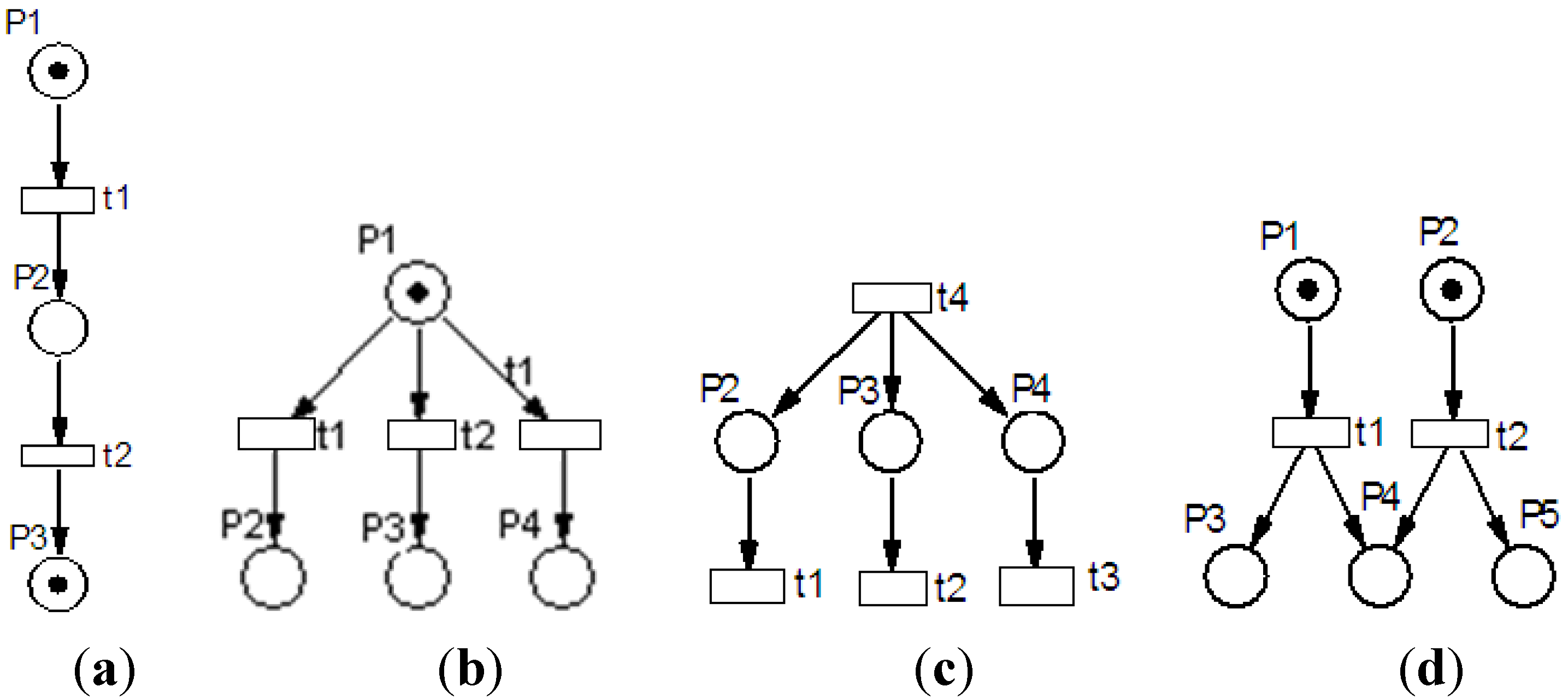
2.1. Definition of the Basic Petri Net

Definition 1: A basic Petri net is composed of hydrophone triplets N = (P,T,F) [15]. Among them, P = {p₁, p₂,…, p_n} is the library set and n is the quantity of libraries. T= {t₁, t₂,…,t_m} is the transition set and m is the quantity of transitions. F = (P * T) ∪ (T * P) is a set of the flow relationships. The system model should include elements of the marking states and those causing the states to be changed. In Petri nets, libraries are state elements. Transitions represent events causing the system state to be changed, such as component faults, maintenance, etc. The arc connecting library and transition represents the flow relationship of state and event. In a graphical model, the library is marked by “○”, token number is marked by a black spot, transition is marked by “□”, and a flow relationship is marked by “→”.

2.2. Basic Properties of a Petri Net

A basic Petri net can express logical relationships among events, such as “AND”, “OR” and “NOT”. It also can analyze system properties, such as accessibility, boundaries, activity, fairness, deadlock and so on. The property not only has a relationship with initial state, but also has a relationship with the structure of the Petri net. The main properties and characteristics are introduced as follows:

Accessibility refers to the designated state which can be achieved in the operating process of a system. State M can reach state M₁ that means of an existing transition sequence σ to satisfy M [σ > M₁.

Boundary (security) reflects the resource variables demand during the operating process of the system. Theoretical analysis will often assume that the capacity of libraries is infinite, but in actual system design, the mark numbers of each library should be less than the capacity of the library in network under any condition so that the system can run normally without spilling phenomena.

Activity indicates that the system can run normally, namely that no deadlocks are present. This property is so important that deadlocks should be avoided in the system design.

Resilience indicates the periodicity and circularity of the system operation.

Fairness reflects the fact that the system is starvation-free. Namely, no starvation phenomenon appears in any of the system partitions when it competes for shared resources.

Reversibility indicates the resilience of system operation. Namely the system can return to the initial state from the current state.

Conservation indicates that resource is restricted in the actual system, namely that it is conservative.

Consistency indicates that no conflict exists between the behaviors of the system. It is important for the parallel system and parallel algorithm.

2.3. Analytical Method of the Petri Net

The analytical methods of a Petri net mainly include the reachable marking graph and coverable tree, state equations and incidence matrixes, language of the Petri net, process of the Petri net and so on. These methods are all based on mathematical foundations.

2.3.1. Reachable Marking Graph and Coverable Tree

Definition 2: Assume Σ = (P,T;F,M₀) is a finite Petri net. A reachable marking graph of Σ is defined as the hydrophone triplets RG(Σ) = (R(M₀),E,f). Among them:

E={(M_i, M_j | M_i, M_j ∊ R(M₀), ∃t_k ∊ T : M_i[t_k > M_j
f : E → T, f(M_i, M_j) = t_k

Only when M_i [t_k > M_j is satisfied, R(M₀) is a vertex set of RG(Σ) and E is an arc set of RG(Σ). If equation f (M_i, M_j) = t_k is satisfied, t_k is side marker of arc (M_i, M_j). For a bounded Petri net, the reachable marking graph can analyze the reachable states, reversibility, activity, fairness and boundary of the library, etc. For unbounded Petri nets, the coverable tree and coverable graph can analyze the boundary and partial activity of Petri nets. Reachable analysis is illustrated in Figure 1.

Figure 1. (a) P/T system (b) Reachable tree T (c) Reachable graph G.

Figure 1. (a) P/T system (b) Reachable tree T (c) Reachable graph G.

2.3.2. Incidence Matrix and Invariant

The incidence matrix can be used to analyze Petri net characteristics without depending on the initial identification, while only having relevance to the net structure. The characteristics are structure boundary, structure equality and repeatability, etc. Invariants contain place invariants (P-invariants) and transition invariants (T-invariants). P-invariants which reflect the weighting conservation of the token numbers of the partial places can be used to research the net deadlock (activity), the mutual exclusion behavior and the error recovery, etc. T-invariants which express possible transition sequences of the state regression can be used to analyze the nets’ periodicity and circularity, etc.

2.3.3. Linguistics Analysis Method

A transition sequence is a string, while a string set is a language. All the transition sequence sets represent a Petri net. The performance of Petri net can be analyzed by transition sequences. The first step of the analytical method is to mark the Petri nets. A transition corresponds to a symbol in the alphabet, so a transition sequence which is corresponding to a language can be used for the standard and auto-synthesis of a Petri net. If the required behavior of a system is described by a language, a Petri net will be automatically synthesized to make the language just be the required behavior language. This Petri net can act as a controller.

2.3.4. Computer Simulation Analysis

As an efficient tool, the computer simulation analysis can also be used for performance analysis of Petri nets. Performances such as boundary, activity, etc., can be analyzed by computer simulation.

2.3.5. Structural Analysis

Structural properties of Petri nets are determined by the nets’ structure rather than the initial identification. Therefore, network performance can be researched by structural boundaries, repeatability, coordination, conservation and relationships among transitions, etc. The relations which have been shown in Figure 2 are the ordinal relation, the conflict relation, the concurrent relation and the impact relation. At present, the structural analysis of Petri nets is used for a class of special nets or a performance of a specific net. In structural analysis, a Petri net with its structure and connection can simplify and refine the system. For a large Petri net through decomposition and using the structure analysis method, we can avoid generating and analyzing all state space, thus avoiding the combination explosion problem.

Figure 2. (a) Ordinal relation (b) Conflict relation (c) Concurrent relation (d) Impact relation.

Figure 2. (a) Ordinal relation (b) Conflict relation (c) Concurrent relation (d) Impact relation.

3. Modeling of a Hydraulic Variable Pitch System Based on the Petri Net

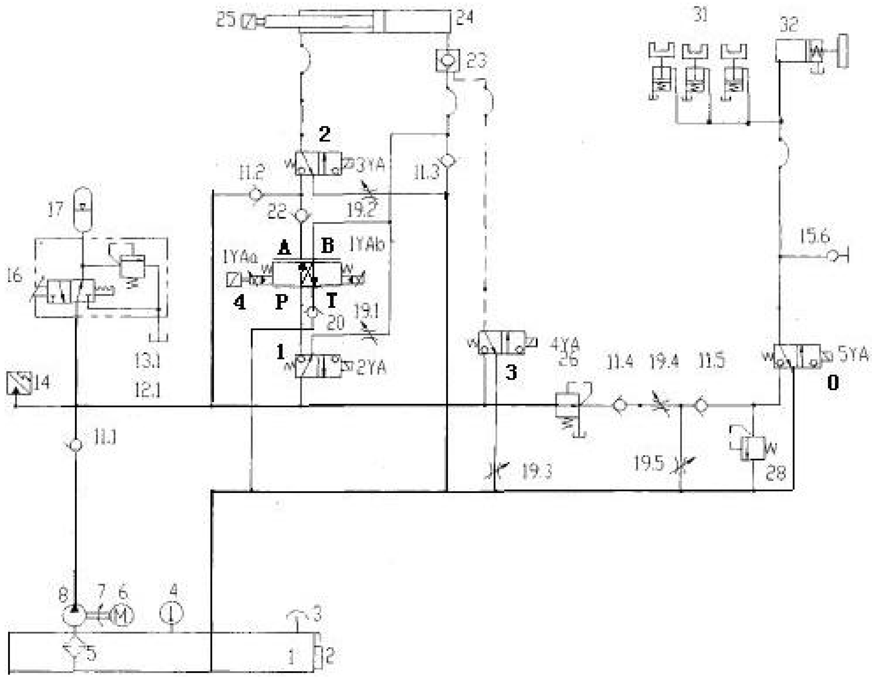
3.1. Working Process of a Hydraulic Variable Pitch System

The hydraulic system of the wind turbines performs the variable pitch operations and the braking to realize the speed control, power control and switching. Taking as an example the schematic diagram of the hydraulic variable pitch system of a VESTAS V39 wind turbine shown in Figure 3, the working process of a hydraulic variable pitch system is introduced as follows [16]:

Figure 3. Schematic diagram of hydraulic variable pitch system of VESTAS V39 wind turbine.

Figure 3. Schematic diagram of hydraulic variable pitch system of VESTAS V39 wind turbine.

Start-up process: after pressing the start-up button, reversing valve (0) is charged with electricity, while other hydraulic valves are not. The brake caliper (32) is opened after overcoming the spring force under the action of hydraulic pressure and the brake is loosed. Hydraulic oil flows into the rod-less cavity (24) of the oil cylinder to adjust the +90° pitch angle through the one-way valve (11.1), electromagnetic reversing valve (1), throttle valve (19.1) and hydraulic operated check valve (23). When the wind velocity reaches the threshold wind velocity, the electromagnetic reversing valves (1), (2) and (3) are charged with electricity. The hydraulic cylinder is regulated by the electric-hydraulic proportional reversing valve (4) to control the paddle pitch angle of the blades. Blades turn to the direction of 0° when the attack angle of the blades caused by airflow reaches a certain angle.

Power regulation process: at this time, electromagnetic reversing valves (1), (2), (3) and the electric-hydraulic proportional reversing valve (4) are charged with electricity. The hydraulically operated check valve (23) is set on two-way conducting library by pilot pressure.

When the wind turbines operate below their rated power, the electric-hydraulic proportional reversing valve (4) is set on “shoot-through” (P–A, B–T). Pressure oil flows into the rod cavity (25) of the hydraulic cylinder through the one-way valve (22) and electromagnetic reversing valve (2). The piston moves right and the blade pitch angle is adjusted to the direction of −5°. Then oil from the rod-less cavity (24) of the hydraulic cylinder backflows into the tank through the hydraulically operated check valve (23), electric-hydraulic proportional reversing valve (4) and one-way valve (20).

When the wind speed is increased causing the output power to increase, the electric-hydraulic proportional reversing valve (4) is set on “cross-modality” (P–B, A–T). Pressure oil flows into the rod-less cavity (24) of the hydraulic cylinder through the hydraulic operated check valve (23). Meanwhile, oil backflows to the pressure pipeline from the rod cavity (25) of the hydraulic cylinder through the electromagnetic reversing valve (2) and one-way valve (11.2).

Normal shutdown process: when a shutdown instruction is sent out, the electromagnetic reversing valve loses electricity. Pressure oil provided by the accumulator (17) and the hydraulic pump flows into the rod-less cavity (24) of the hydraulic cylinder through the electromagnetic reversing valve (1), throttle valve (19.1) and hydraulic operated check valve (23). Oil left in the hydraulic cylinder is discharged into the tank through the electromagnetic reversing valve (2) and throttle valve (19.2). When the blade pitch angle reaches +88 °, rotor speed is reduced and the reversing valve (0) loses electricity. Oil in the brake flows back to tank and the brake is locked under the action of spring force to brake the rotor.

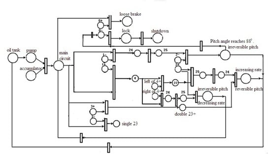
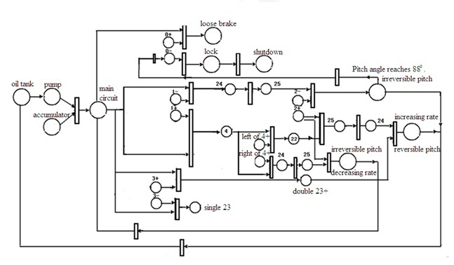
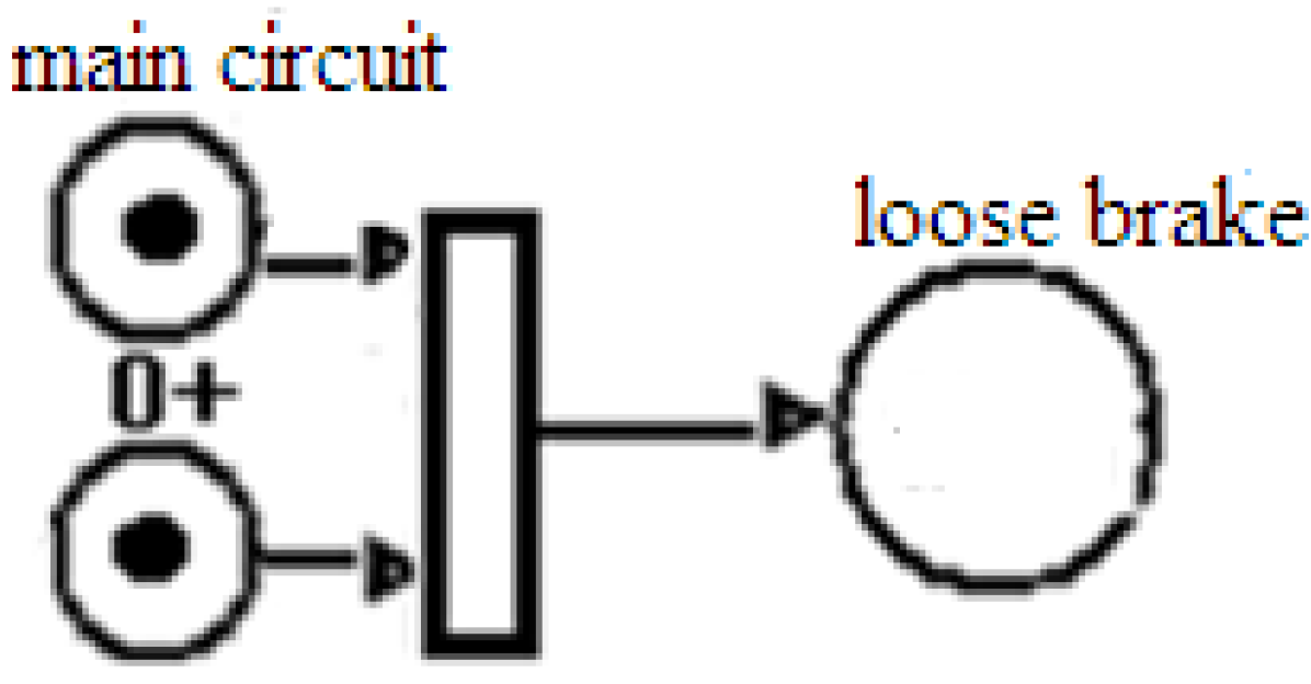
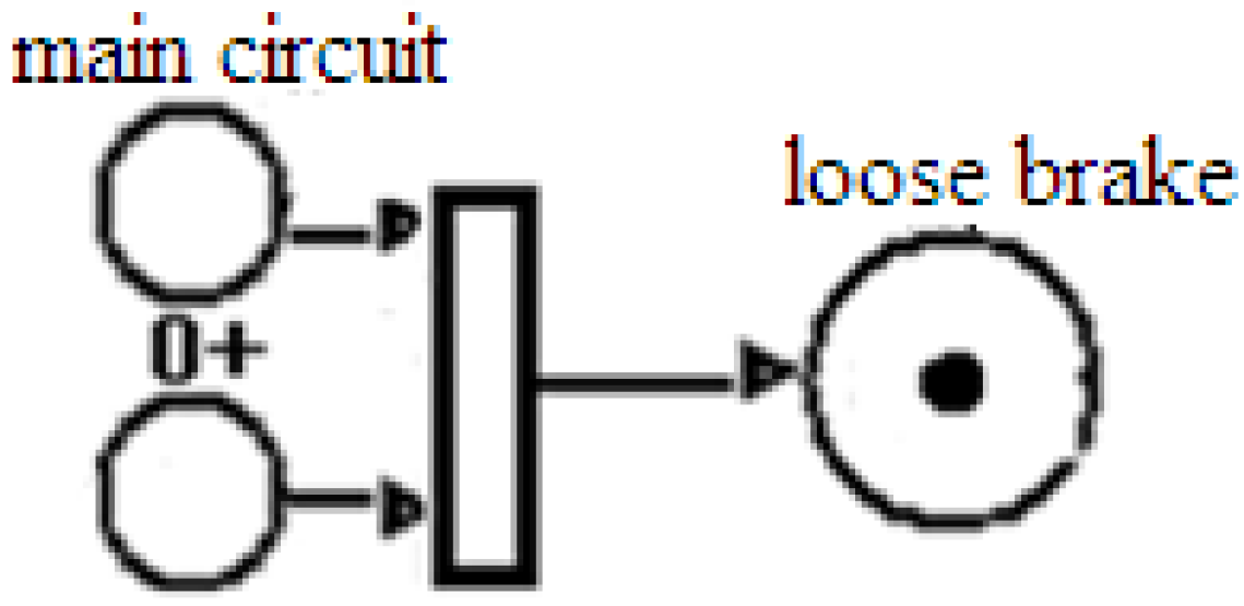
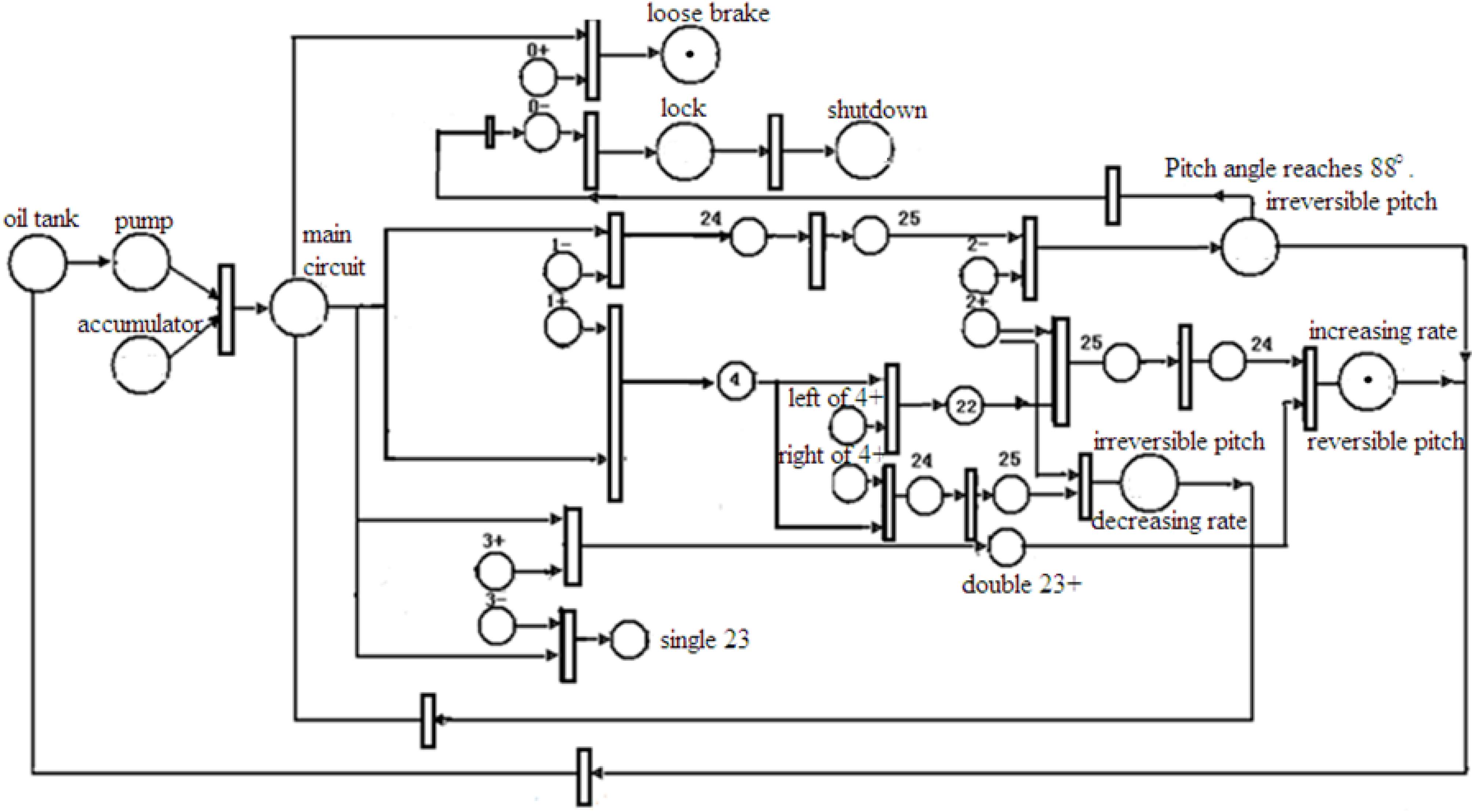
3.2. Basic Petri Net Model of a Hydraulic Variable Pitch System

The Petri net is composed of library, transition, tokens and the directional arc which is used to connect library and transition. The Petri net is a modeling method which can reveal a system’s structure and dynamic behavior with graphs. In these, the library is represented by a round knot, transition is represented by a rectangular knot, token is represented by a small black spot and directional arc is represented by a directed arrow. When a library contains a token, the library and its token will constitute a system logo. If a transition is pointed by all libraries which contain at least a token, the transition is a possible occurrence. If the transition is possible and the external logic conditions which make it happen are satisfied, the transition can launch. After the transition launch, a token is retrieved from each input library of the transition and a token is set in each output library of the transition. Then the system is on a new logo state [17].

Through analyzing whether the main electromagnetic valves are charged with electricity and logical relations among the working states of hydraulic variable pitch system, the basic Petri net of the hydraulic variable pitch system is obtained according to the basic principles of the Petri net. The corresponding figure is shown as Figure 4.

Figure 4. Basic Petri net of a variable pitch system.

Figure 4. Basic Petri net of a variable pitch system.

According to the working principle of the Petri net model, Figure 4 can represent whether the main electromagnetic valves are charged with electricity and logical relations among the working states of hydraulic variable pitch system. The working principles are analyzed as follows:

When the system is running normally, “main circuit” will contain a token.

Loose brake: Reversing valve (0) is charged with electricity and oil flows into the brake caliper (32). At this time, reversing valve (0) is charged with electricity and library “0+” contains a token. The “main circuit” library also contains a token. The states are as shown in Figure 5. When library “0+”and library “main circuit” all contain tokens, the “loose brake” library will contain a token. The states are shown as Figure 6. At this time, the loose braking action is finished.

Figure 5. Before transfer.

Figure 5. Before transfer.

Figure 6. After transfer.

Figure 6. After transfer.

Start-up and increasing power: in order to make the pole move correctly, it should work on the reversible pitch process. Electromagnetic reversing valves (1), (2), (3) and the left side of the electric-hydraulic proportional reversing valve (4) are charged with electricity. It works on the “shoot-through” state (P–A, B–T).

When the electromagnetic reversing valves (1), (2), (3) and the left side of the electric-hydraulic proportional reversing valve (4) are charged with electricity, these corresponding libraries all contain tokens. The states as are shown by Figure 7. When the “main circuit” library and “1+” library all contain tokens, library “4” will contain a token. Meanwhile the “left of 4+” library contains a token. Then library “22” contains a token. Library “22” and library “2+” containing tokens leads to library “25” containing a token. Then library “24” contains a token. At the same time, the “main circuit” and “3+” libraries contain tokens to lead to the “double 23+” library containing a token. Libraries of “double 23+” and “24” jointly have tokens, which makes the “increasing rate” library contain a token. The states are as shown in Figure 8. Then, the system will complete the process of start-up and increasing power.

Figure 7. Before transfer.

Figure 7. Before transfer.

Figure 8. After transfer.

Figure 8. After transfer.

Decreasing power: in order to make the pole move to the left, it should work on the irreversible pitch process. Electromagnetic reversing valves (1), (2), (3) and the right side of electric-hydraulic proportional reversing valve (4) are charged with electricity. It works on the “cross-modal” state (P–B, A–T) which is called the differential circuit. At this time, electromagnetic reversing valves (1), (2), (3) and the right side of the electric-hydraulic proportional reversing valve (4) are charged with electricity. Libraries “main circuit”, “1+” and “4” contain tokens. Libraries “4” and “right of 4+” contain tokens, which lead to libraries “24” and “25” containing tokens. Meanwhile, libraries “2+” and “decreasing rate” contain tokens. Then it will complete the process of decreasing power.

Shutdown: this is an irreversible pitch process and the electromagnetic reversing valves (1), (2), (3) and electric-hydraulic proportional reversing valve (4) lose electricity. When the pitch angle reaches +88°, the reversing valve (0) will lose electricity and the braking device will be locked.

Now none of the valves will be electricified. Libraries of “1−” and “main circuit” contain tokens, which leads to libraries “24” and “25” containing tokens. At the same time, library “2−” also contains a token to make the library of “irreversible pitch” contain a token. When the transition reaches the condition that pitch angle is 88°, reversing valve (0) will lose electricity and library “0−” contains a token to make library "lock" contain a token. This will complete the shutdown process.

The Petri net can represent each state of the abstract and discrete system with images and concrete models. It has graphical modeling and mathematics calculation capacity. The Petri net is unique in the system description and dynamic performance analysis [18].

4. Modeling Based on the Fault Petri Net of a Hydraulic Variable Pitch System

Petri nets reveal the structure and dynamic behavior of a system and establish the system’s model with graphical language. The fault diagnosis method based on Petri nets combines the knowledge representation with the diagnosis reasoning to complete the diagnosis reasoning of descriptive knowledge and process. In the fault detection and diagnosis field, Petri nets can be used to express the system logic relation and to complete the knowledge representation and the diagnosis reasoning. It also can be used to establish behavior model for diagnosed object and to use attribute of Petri nets to do model-based diagnosis reasoning.

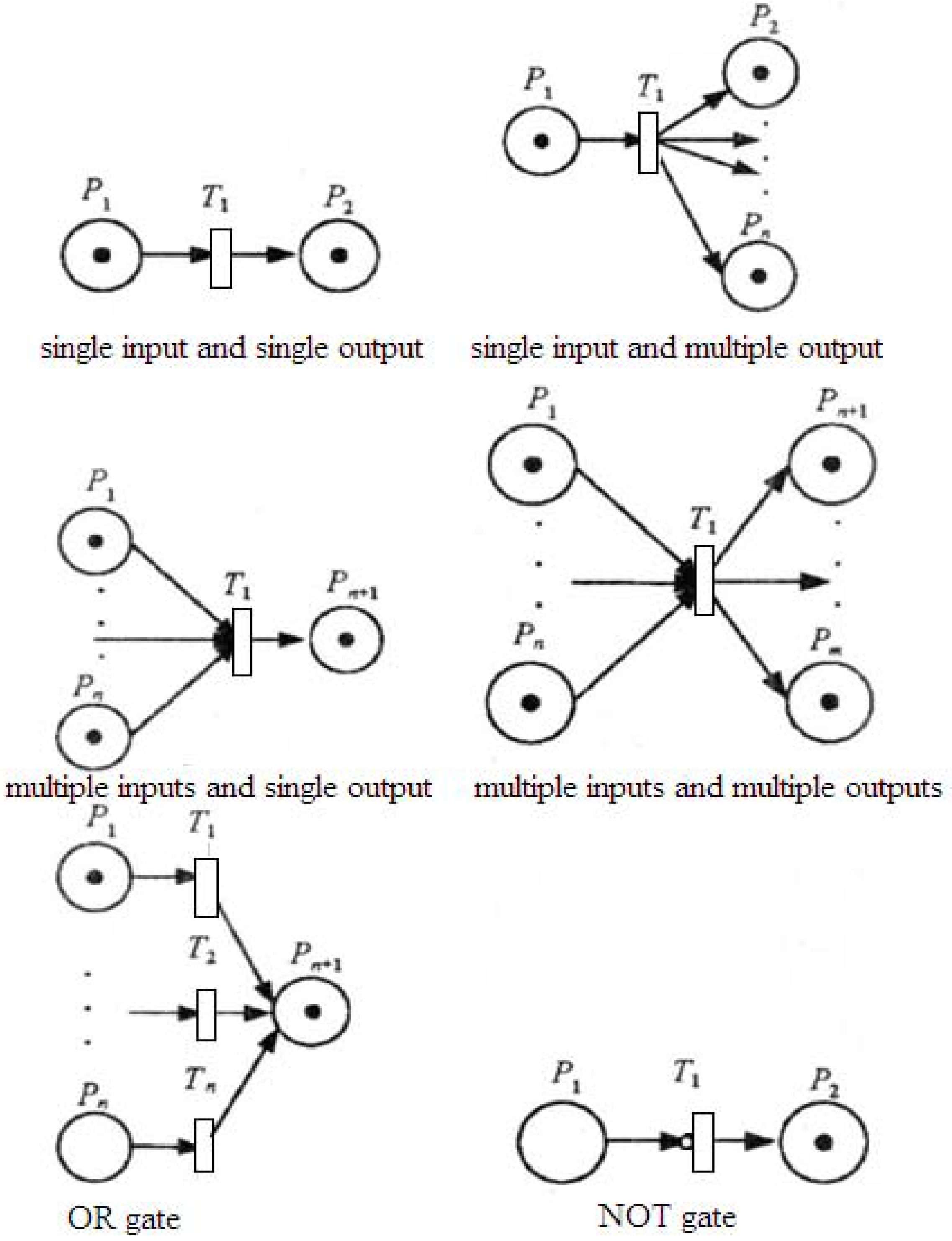
4.1. Difference between Fault Tree and Fault Petri Net

A fault tree is a special kind of a tree shape logic causality diagram that by setting events, logic gates and other symbols describes the causal relationships of various events. Fault tree analysis (FTA) is a useful tool of reliability analysis of large and complex systems, but as a kind of traditional system reliability analysis tool, the FTA method does not involve a large number of properties of dynamic system in engineering practice, so with the FTA approach it is difficult to describe and evaluate reliability problems of dynamic system including repair or control. In fault diagnosis, Petri nets have a series of advantages, such as fast reasoning and mathematical diagnosis process. Petri nets make full use of their mathematical foundations and convert diagnosed problems into mathematical matrix operations. A Petri nets model is similar to a fault tree. The graphical representation based on Petri nets model, can effectively describe the reason and relationships of events, focus on expressing the transmission relationships of various faults, and ignore the time factor. That is to say, the transitions of fault Petri nets are instant transitions. When all the input libraries contain tokens, transitions will be triggered immediately. According to the logical relationship based on fault Petri nets, the logic gates of fault Petri nets are different from the logic gates of fault trees. The differences are shown in Table 1.

Table 1. Logic representation of fault tree and corresponding fault Petri net.

Logical Relationship	Fault Tree Model	Petri Net Model
Logic OR Gate
Logic AND Gate
Logic BAN Gate
Logic NOT Gate

Table 1. Logic representation of fault tree and corresponding fault Petri net.

Logical Relationship	Fault Tree Model	Petri Net Model
Logic OR Gate
Logic AND Gate
Logic BAN Gate
Logic NOT Gate

4.2. Fault Diagnostic Principle Based on Fault Petri Net

The fault diagnostic technique based on fault Petri nets is based on a graph theory model. It combines the diagnosis problem based on the model with its property and reach-ability analysis. Using graphic language, Petri nets, which can analyze and describe the structure, function and process of the fault diagnosis system, have been applied more and more in the fault diagnosis field [19].

In Petri nets, a library represents a system event, a mark represents an event state and a transition represents a kind of relationship between libraries. We take the system fault as a top place and the system working state and the fault reason as a basic place. Then the fault Petri net model can be established. The fault diagnosis process can resemble a dynamic transition of the system state. Namely, we determine the transition process which leads to the top library being marked and the process of marking the system transition. Malfunction omens are represented by the input library and fault type is represented by the output library in the Petri net. When the input library contains a token, it will mean that a malfunction omen has occurred. When the output library contains a token, it will mean that a fault occurs. The fault diagnosis process is a process to obtain a network initial logo state according to the appearing malfunction omens and to transfer tokens to the output libraries through a series of transition launches. When output libraries contain tokens, the network will get new logo states. It means that the corresponding faults occur when the output libraries contain tokens.

The fault diagnosis process based on fault Petri nets is as follows: we establish a fault Petri net model which reflects the relationship of system faults, system working state and causes for the breakdown. Next, we determine the initial state of the system (namely, the initial mark). We determine whether the top library has been marked or not by the solution of the dynamic transition of the system state based on the Petri net model. If the top place has been marked that means there is a system fault.

Figure 9. Fault Petri net model of a hydraulic variable pitch system.

Figure 9. Fault Petri net model of a hydraulic variable pitch system.

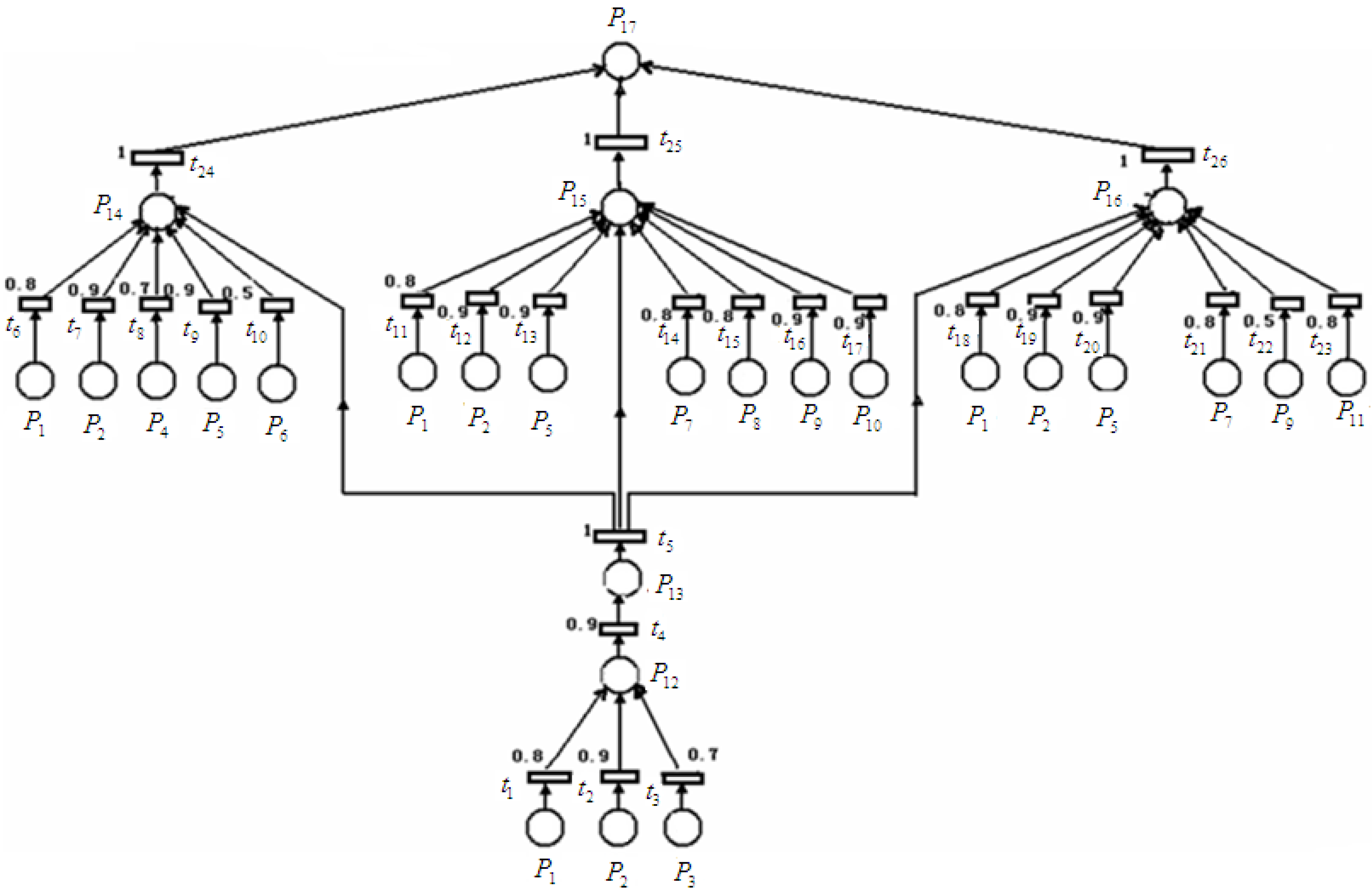
4.3. Modeling of the Fault Petri Net of a Hydraulic Variable Pitch System

In order to establish a fault Petri net model, the first thing is to determine the top events of the fault model, which are also called fault criteria. Fault criteria of a hydraulic variable pitch system are start-up faults, increasing power faults and decreasing power faults. The three criteria constitute the first level events of the fault Petri net model for a hydraulic variable pitch system. Analyzing the first level events, we find out the direct reason of each event which has happened and the logical relationship among fault sources. According to this method, the bottom fault source causing a system fault will be detected. The fault Petri net model of a hydraulic variable pitch system is shown in Figure 9. The meaning of each library in Figure 9 is shown in Table 2. The overhaul cycle of the hydraulic variable pitch system of wind turbines is about 5000 hours. In the life cycle, each probability of the bottom event is shown in brackets after the sequence number.

Table 2. Meaning and fault probability of each component place of hydraulic variable pitch system.

Positions of Bottom Events	Meaning of Positions	Middle Positions	Meaning of Middle Positions
P1 (0.0005)	Hydraulic pump provides less oil	P12	Pressure of return circuit is not enough, when brake is loosed
P2 (0.0005)	Pressure of accumulator is not enough	P13	The failure of loosing brake
P3 (0.06)	Sealing is not good after valve 0 is charged with electricity	P14	The fault of irreversible pitch on the process of start-up
P4 (0.036)	Valve 1 is not charged with electricity or 19.1 leaks oil	P15	The fault of increasing power or reversible pitch
P5 (0.01)	Piston is seriously abraded	P16	The fault of decreasing power or irreversible pitch
P6 (0.036)	Valve 2 is not charged with electricity or 19.2 leaks oil	P17	The fault of variable pitch for hydraulic variable pitch system
P7 (0.05)	The state fault of valve 1 with electricity
P8 (0.06)	The fault of valve 4 set on shoot-through
P9 (0.05)	The state fault of valve 2 with electricity
P10 (0.02)	Valve 3 leaks oil or double 23 is fault
P11 (0.06)	The state fault of valve 4 set on the cross-modality

Table 2. Meaning and fault probability of each component place of hydraulic variable pitch system.

Positions of Bottom Events	Meaning of Positions	Middle Positions	Meaning of Middle Positions
P1 (0.0005)	Hydraulic pump provides less oil	P12	Pressure of return circuit is not enough, when brake is loosed
P2 (0.0005)	Pressure of accumulator is not enough	P13	The failure of loosing brake
P3 (0.06)	Sealing is not good after valve 0 is charged with electricity	P14	The fault of irreversible pitch on the process of start-up
P4 (0.036)	Valve 1 is not charged with electricity or 19.1 leaks oil	P15	The fault of increasing power or reversible pitch
P5 (0.01)	Piston is seriously abraded	P16	The fault of decreasing power or irreversible pitch
P6 (0.036)	Valve 2 is not charged with electricity or 19.2 leaks oil	P17	The fault of variable pitch for hydraulic variable pitch system
P7 (0.05)	The state fault of valve 1 with electricity
P8 (0.06)	The fault of valve 4 set on shoot-through
P9 (0.05)	The state fault of valve 2 with electricity
P10 (0.02)	Valve 3 leaks oil or double 23 is fault
P11 (0.06)	The state fault of valve 4 set on the cross-modality

5. Reliability Analysis of a Fault Petri Net

5.1. Qualitative Analysis of a Fault Petri Net

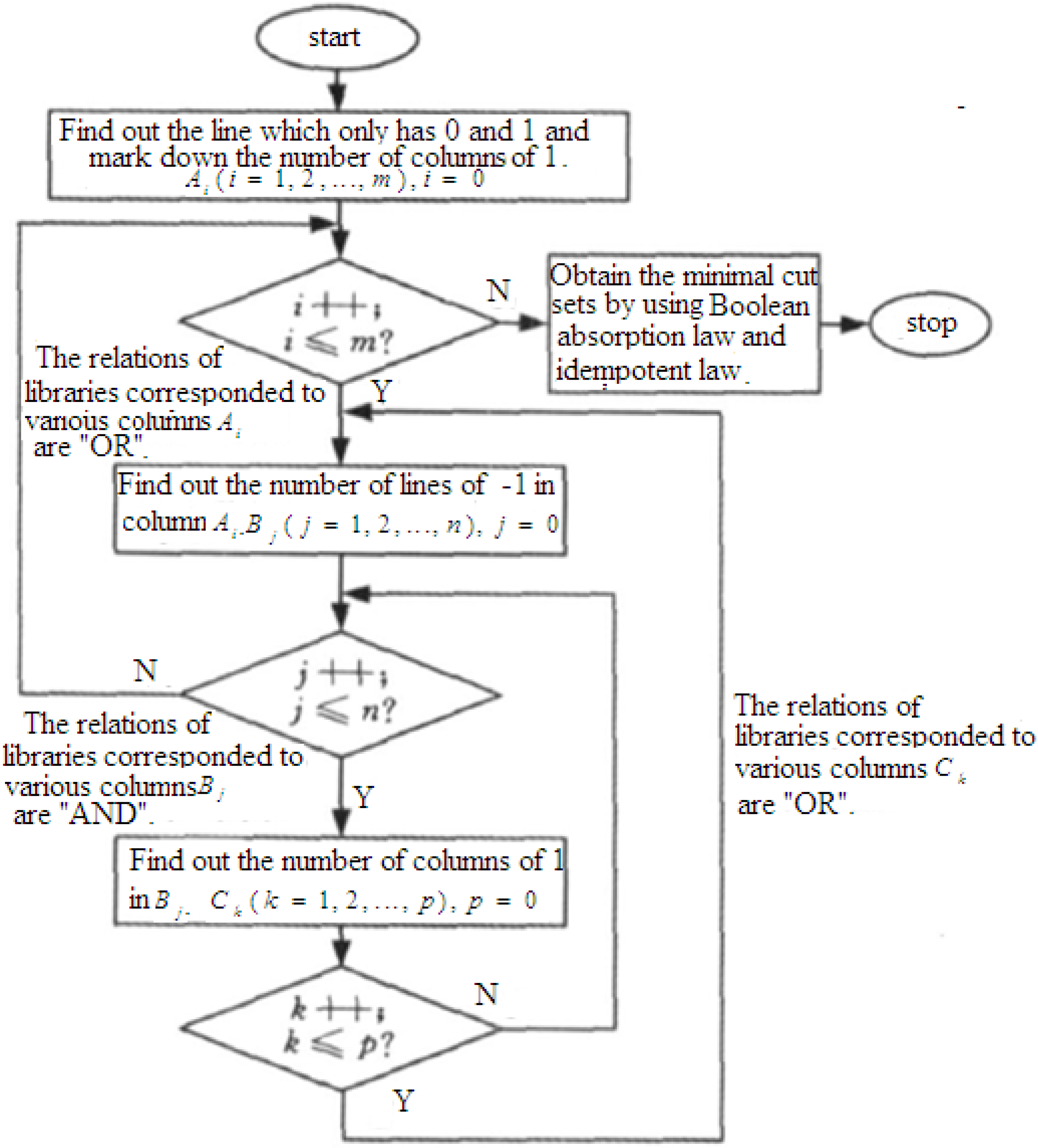
The qualitative analysis task of the fault Petri net is to find all the possible fault modes and when the state combinations causing top events (system faults) occurred. That is to say, find out all minimum cut sets of the fault Petri net. A minimum cut set contains the minimum quantity and the most necessary bottom events. If each bottom event occurs in the cut set, a top event will happen. Each cut set of the fault Petri net represents one kind of possible fault or failure mode. All the minimum cut sets of the fault Petri net represent all possibilities of top events happening. The whole minimum cut sets are the whole fault models. Minimum cut sets can reflect basic system faults which should be necessarily repaired and reflect the weakest link [20].

The minimum cut set of a fault Petri net is not only one. Finding out all minimum cut sets of the system is a significant task. According to the minimum cut sets, one can pertinently improve system design and create a maintenance strategy by using the most reasonable methods to enhance the system reliability level. The incidence matrix is one of main analytical methods. In a fault Petri net, input matrix I and output matrix O all can be represented by the nonnegative integer matrix n × m. The difference between the output matrix O and the input matrix is called the incidence matrix [21,22]. The difference can be represented by A^T (A^T = O − I). Next we can take Figure 10 as an example to seek out an incidence matrix.

Figure 10. Petri Net Model.

Figure 10. Petri Net Model.

From Figure 10, the input matrix can be shown as Formula (1) and the output matrix can be shown as Formula (2):

(1)

(2)

Then its incidence matrix can be represented by Formula (3):

(3)

According to above method, in Figure 9 the incidence matrix of the fault Petri net model of a variable pitch system can be shown as follows:

According to the incidence matrix, the step to seek out minimum cut sets can be as shown below:

(1)

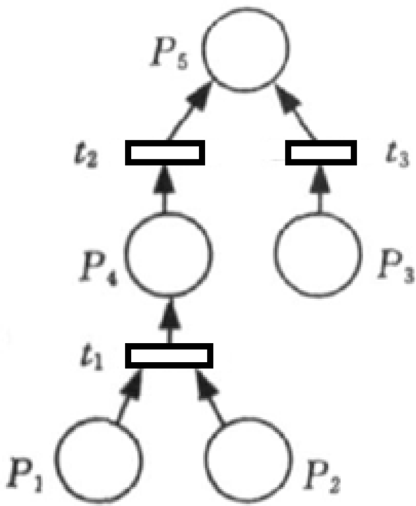
In the incidence matrix, find out the line which contains only 0 s and 1 s without −1 s. Then the library corresponding to that line is the top library. Start to search from this top library.

(2)

From 1 in the corresponding line of top library, −1 can be searched by column. Then the library which is represented by the corresponding line of −1s is an input library of the top library. If the column has multiple −1 s, the same transition will have multiple input libraries and these input libraries have an “AND” relationship.

(3)

According to the −1 which is searched by step (2), continue to search 1 by line. If there is a 1, the corresponding library is a middle library. Continue to search circularly as in step (2), until no 1s are found in the line. If there is no the line of 1s, the library will be a bottom library called basic event. If there are multiple 1s in a corresponding line, the corresponding library will have multiple transitions. From the corresponding line of 1 as step (2), find out the lines of −1 s. The corresponding libraries of these lines have the relationship of “OR”.

(4)

Continue to search as step (2) and step (3), until the most bottom libraries are found.

(5)

According to the above relationship of “AND” and “OR”, spread these bottom libraries and then get all cut sets.

(6)

Obtain minimum cut sets through Boolean absorption law, idempotent law and prime number method.

According to the above steps, we can compile a computer program as shown in the program flow chart of Figure 11. Use VC++ language to compile the below program:

(1)

Define a planar array to express the incidence matrix;

(2)

Transfer recursive function to search −1 by column and 1 by line;

(3)

Use a loop statement to express the relationship among cut sets.

Figure 11. Program flow chart.

Figure 11. Program flow chart.

According to the above method, all the minimum cut sets of the fault Petri net model of the wind turbine hydraulic variable pitch system are {P₁}, {P₂}, {P₃}, {P₄}, {P₅}, {P₆}, {P₇}, {P₈}, {P₉}, {P₁₀}, {P₁₁}.

In order to verify the correctness of above method, we will use another method to find the minimum cut sets. Liu, Chiou and others have proposed a minimum cut set matrix and non-intersect minimum cut set algorithm [23]. The steps of how this algorithm looks for minimum cut sets are as follows: (1) If an output library through multiple arcs is linked with many transitions, input libraries are marked by numbers in the form of a level arrangement; (2) If an output library is linked with a transition through a single curve, the input library is marked by numbers in the form of a perpendicular arrangement; (3) Middle libraries are instead of subordinate level to establish library array. If a library of public numbers exists between row and column, these libraries will be shared by row and column. The column of the array is cut set; (4) Removing a superset one can get minimum cut set. According to this method, all the minimum cut sets of the fault Petri net model for the wind turbine hydraulic variable pitch system are {P₁}, {P₂}, {P₃}, {P₄}, {P₅}, {P₆}, {P₇}, {P₈}, {P₉}, {P₁₀}, {P₁₁}. Comparing these two methods, we can easily conclude that the first method based on Visual C++ 6.0 is not only correct, but also more convenient for finding the minimal cut sets of the fault Petri net.

5.2. Quantitative Calculation of the Fault Petri Net

The fault Petri net is composed of seven-elements (P, T, I(t_j), O(t_j), f(I)_i, f(O)_j, μ_j). Among them, the finite set of libraries P = {p₁, p₂,…, p_n} expresses the fault state of components and system. The finite set of transitions T = {t₁, t₂,…, t_m} expresses the transfer process of fault states. Input function I(t_j) = p_i expresses the directional arc from library p_i to transition t_j. The input position of transition t_j is library p_i. The output function O(t_j) = p_i expresses the directional arc from transition t_j to library p_i. The output position of transition t_j is library p_i. f(I)_i is the failure probability set of the input function. f(O)_j which is the failure probability set of the output function is determined by the failure probability of the input function. μ_j is the incidence of transition t_j.

According to the logic relationship of fault events, basic models of fault Petri nets are single input and single output, single input and multiple output, multiple inputs and single output, multiple input and multiple output, NOT gate and OR gate. A fault Petri net model is composed of various minimal unit models. Various minimal unit models have been shown in Figure 12.

Fault logical relationships of engineering machinery hydraulic systems manifest the relationships of “and” and “or”. Transitions are mainly multiple input and single output, single input and single output.

For an output library of transitions with multiple inputs and a single output, the transition will occur only when all library conditions are satisfied. At this time, the failure probability set of the output function is shown by Formula (4):

(4)

For an output library of transition with a single input and a single output, the failure probability set of the output function is shown by Formula (5):

(5)

If the output library has transitions which have the numbers of k, the failure probability set of the output function is shown by Formula (6):

(6)

For an actual system, after establishing a fault Petri net model of the system, if the occurrence probabilities of all bottom events are known, the fault rate of any knot in the fault Petri net model will be obtained by using Formulas (4), (5) and (6). According to the fault Petri net model of the variable pitch system in Figure 9, a transition represents a single input and a single output, so the fault rate can be obtained by Formulas (5) and (6). For an overhaul period of 5000 hours, various fault probabilities of the system will be obtained by the fault probabilities of bottom events in Table 2. The fault probability of library P₁₂ is 0.038. The fault probability of P₁₄ is 0.09. The fault probability of P₁₅ is 0.18. The fault probability of P₁₆ is 0.14. The probability of the system top events (hydraulic variable pitch system fault) P₁₇ is 0.35. Therefore, the reliability of the hydraulic variable pitch system of wind turbines is 0.65.

Figure 12. Minimal unit model of a fault Petri net.

Figure 12. Minimal unit model of a fault Petri net.

6. Conclusions

In this paper, Petri net theory is adopted to build a model for each discrete state of the hydraulic pitch system operation process in wind turbines and a fault Petri net model is established at the same time. Through qualitative analysis and quantitative calculation, the system reliability index is obtained and it provides important references for the performance of the system. Not only does the Petri net describe the structure, function and process through a graphical language, but also the fault Petri net model can clearly express the logical relations among faults. The fault Petri net model has simple calculation and a broad application prospects. The reliability estimation based on a Petri net has provided a theoretical basis for determining the reliability of a hydraulic variable pitch system.

References

1. Galdi, V.; Piccolo, A.; Siano, P. Designing an adaptive fuzzy controller for maximum wind energy extraction. IEEE Trans. Energy Convers. 2008, 23, 559–569. [Google Scholar] [CrossRef]
2. Calderaro, V.; Galdi, V.; Piccolo, A.; Siano, P. A fuzzy controller for maximum energy extraction from variable speed wind power generation systems. Electr. Power Syst. Res. 2008, 78, 1109–1118. [Google Scholar] [CrossRef]
3. Galdi, V.; Piccolo, A.; Siano, P. Exploiting maximum energy from variable speed wind power generation systems by using an adaptive Takagi-Sugeno-Kang fuzzy model. Energy Convers. Manag. 2009, 50, 413–421. [Google Scholar] [CrossRef]
4. Ye, H.Y. Actuator of control system. In Control Technology of Wind Turbines; Ye, H.Y., Ed.; China Machine Press: Beijing, China, 2006; Volume 7, pp. 111–131. [Google Scholar]
5. Liu, X.; Zhang, X.M. Dynamic simulation of the supervisory control of variable speed pitch regulated wind turbines. Acta Energ. Sol. Sin. 2008, 29, 1008–1013. [Google Scholar]
6. Zhao, W.Z.; Qin, L.X.; Yao, X.J. Modeling research of MW wind turbine variable pitch system. Mach. Tool Hydraul. 2006, 6, 157–162. [Google Scholar]
7. Georgilakis, P.S.; Katsigiannis, J.A.; Valavanis, K.P.; Souflaris, A.T. A systematic stochastic Petri net based methodology for transformer fault diagnosis and repair actions. J. Intell. Robot. Syst. 2006, 45, 181–201. [Google Scholar] [CrossRef]
8. Katsigiannis, Y.A.; Georgilakis, P.S.; Tsinarakis, G.J. A novel colored fluid stochastic Petri net simulation model for reliability evaluation of wind/PV/diesel small isolated power systems. IEEE Trans. Syst. Man Cybern. Syst. Hum. 2010, 40, 1296–1309. [Google Scholar] [CrossRef]
9. Wu, Q.D.; Yan, J.W.; Zhang, H. Principle and Practical of Flexible Manufacturing Automation; Wu, Q.D., Yan, J.W., Zhang, H., Eds.; Tsinghua University Press: Beijing, China, 1997. [Google Scholar]
10. Ciardo, G.; Trivedi, K.S. A decomposition approach for stochastic Petri net models. In Fourth International Workshop of Petri Nets and Performance Models; Petri Nets and Performance Models: Melbourne, Australia, December 1991; pp. 74–83. [Google Scholar]
11. Berthelot, G.; Terrat, R. Petri nets theory for the correctness of protocols. IEEE Trans. Commun. 1982, COM-30, 2497–2505. [Google Scholar]
12. Kasai, T.; Miller, R.E. Homomorpisms between models of parallel computation. J. Comput. Syst. Sci. 1982, 25, 285–331. [Google Scholar] [CrossRef]
13. Genrich, H.J.; Thiagarajan, P.S. Atheory of bipolar synchronization schemes. Theoret. Comput. Sci. 1984, 30, 241–318. [Google Scholar] [CrossRef]
14. Wang, Q.; Zhang, W.J.; Sun, B.; Yang, R.Q. Object-oriented and Petri-net based simulation for robotic assembly system. Modul. Mach. Tool Autom. Manuf. Technol. 2002, 2, 5–7. [Google Scholar]
15. The Theory of Petri Net; Yuan, C.Y. (Ed.) Electronic Industry Press: Beijing, China, 1998.
16. Lin, Y.G.; Li, W. Study on the technology of pitch-control for large scale wind turbines. PhD Thesis, Zhejiang University, Hangzhou, China, 2005. [Google Scholar]
17. Wang, S.J.; Su, C.; Xu, Y.Q. Research on a hydraulic system’s reliability based on stochastic Petri net and Monte Carlo simulation. Mech. Sci. Technol. 2006, 10, 1206–1209. [Google Scholar]
18. Allard, B.; Morel, H.; Chante, J.P. Power electronic circuit simulation using bond graph and Petri network techniques. In Proceedings of the IEEE Annual Power Electronics Specialists Conference, Seattle, WA, USA, June 1993; pp. 27–32.
19. Portinale, L. Petri net reachability analysis meets model-based diagnosis and problem solving. In Proceeding of the IEEE International Conference on Systems, Man and Cybernetics, SMC 95, Vancouver, Canada, October 1995; pp. 1712–1717.
20. Su, C.; Shen, G.; Xu, Y.Q. Failure analysis and reliability evaluation of mono-bucket excavator’s hydraulic system. Lift. Transp. Mach. 2007, 1, 10–15. [Google Scholar]
21. Application of Petri Net in Modelling and Control of Manufacturing System; Jiang, Z.B. (Ed.) China Machine Press: Beijing, China, 2004.
22. Wang, H.Q. System reliability analysis based on Petri net. Beijing Inst. Light Ind. 1998, 16, 87–93. [Google Scholar]
23. Liu, T.S.; Choiu, S.B. The Application of Petri Nets to Failure Analysis. Reliab. Eng. Syst. Saf. 1997, 57, 129–142. [Google Scholar] [CrossRef]