A General Mathematical Framework for Calculating Systems-Scale Efficiency of Energy Extraction and Conversion: Energy Return on Investment (EROI) and Other Energy Return Ratios

Abstract

The efficiencies of energy extraction and conversion systems are typically expressed using energy return ratios (ERRs) such as the net energy ratio (NER) or energy return on investment (EROI). A lack of a general mathematical framework prevents inter-comparison of NER/EROI estimates between authors: methods used are not standardized, nor is there a framework for succinctly reporting results in a consistent fashion. In this paper we derive normalized mathematical forms of four ERRs for energy extraction and conversion pathways. A bottom-up (process model) formulation is developed for an n-stage energy harvesting and conversion pathway with various system boundaries. Formations with the broadest system boundaries use insights from life cycle analysis to suggest a hybrid process model/economic input output based framework. These models include indirect energy consumption due to external energy inputs and embodied energy in materials. Illustrative example results are given for simple energy extraction and conversion pathways. Lastly, we discuss the limitations of this approach and the intersection of this methodology with “top-down” economic approaches.

1. Introduction

The overall efficiency of our energy extraction and conversion systems strongly influences the economics of energy supply and the environmental impacts of the energy consumed by end users. This “systems scale” efficiency of energy production and processing is difficult to conceptualize and difficult to measure rigorously.

Net energy analysis (NEA) is a broad class of methods used to determine the effectiveness of energy capture and conversion systems [1]. In this sense, NEA is the systems-scale analog to efficiency analysis of technologies. The end result from NEA is often an energy return ratio (hereafter ERR), which compares the amount of energy consumed in extracting an energy resource to the amount of valuable energy provided to society (or to the next stage in the energy processing chain if a tighter system boundary is used). For example, a gas turbine might be characterized by a well-defined conversion efficiency (e.g., MJ electricity/MJ natural gas input, LHV basis), while the efficiency of a natural gas extraction, processing, and distribution pathway can be measured using an ERR. Numerous ERRs exist, and the usefulness of a given ratio depends on its formulation and the question of concern.

Net energy analysis rose and then fell from favor in the energy analysis community, with high interest occurring from ≈1975–1985 and again in recent years [1]. One factor in the declining interest in NEA in the 1980s were concerns that an ERR provides no additional information beyond economic analyses [2]. Also, NEA faced methodological difficulties without clear solutions. Recent interest has been spurred by concerns over oil depletion [3,4] and interest in the fundamental energetics of the transition to renewable resources [5,6]. This recent resurgence in interest in NEA sees current attention focused on a specific ERR known as the energy return on investment, or EROI [7].

In this paper we develop a general mathematical framework for calculating ERRs in a bottom-up fashion. We generate formulas for four ERRs for a general n-stage energy extraction and conversion pathway with varying system boundaries. These ERRs are calculated using both magnitudes of flows (a “flow-based” formulation) and processing efficiencies (an “efficiency-based” formulation). We then compute ERRs for simple illustrative conversion pathways, showing that the results conform to those expected from intuition. Lastly, we discuss the limitations of this approach and discuss extensions such as multi-fuel pathways and integration with top-down economic modeling.

2. Energy Ratios and Their Uses

2.1. Development of Energy Return Ratios

The net energy output from an energy extraction and conversion pathway is the energy made available from a natural resource in useful form less that energy consumed in extracting, upgrading, and distributing the energy [1]. Net energy analysis (NEA) seeks to compare this net output to the energy consumed in producing the output.

Historically, Hall developed the concept of energy return on investment (EROI) and applied it to migrating fish populations [8]. Other roots of NEA include the work of Odum on power flows in social and environmental systems [9]. An early formal framework was developed by the Colorado Energy Research Institute (CERI) [10], which outlined pathways (“trajectories” in their terminology) of energy conversion processes (“modules”) with a variety of primary energy input types. In the CERI framework, there are two types of inputs to each module: principal energy, or the energy resource undergoing extraction and refining, and external energy, or other energy types consumed in the pathway. Also, there are two types of energy that emerge from a given process: energy products, which represent the useful modified principal energy stream, and energy losses, which are outputs of energy in non-useful forms (waste heat or physical loss of product).

Later, Spreng illustrated a simple case of gross vs. net energy requirements in a one-energy-resource economy [11] (p. 132). Similar diagrams were developed by Hannon [12] and others. In these simple NEA models, there is only one energy type, and the extraction and refining of energy consumes energy of that type. This formulation can be used to construct “self net-energy ratios”, which assume that the process provides its own direct and indirect energy inputs.

A variety of complexities and additions to NEA models have been made over time, including differentiating the fractions of fossil and renewable energy used in a process [13], and including temporal aspects of energy return over time [12]. Recently, Spitzley and Keoleian [13] listed numerous published definitions of energy return ratios, starting with the work of Odum in the early 1970s, in a review focused on ratios that differentiate between fossil and renewable energy inputs. Modern efforts to standardize NEA methodologies have focused on standardization of EROI [14,15].

2.2. The Usefulness of Energy Return Ratios

Energy return ratios give different information depending on their formulation. For example the net energy ratio (NER) has as its numerator net output of refined energy to society, while the denominator contains all energy consumed in the energy production and refining process. In contrast, the denominator of the net external energy ratio (NEER) includes only those inputs that are consumed from the existing industrial energy system, excluding any “self use” (e.g., produced oil burned on site to power oil producing operations). Therefore, the NER is a more comprehensive measure of the total energy return from a production pathway, and will be closely correlated with environmental impacts of a pathway (such as greenhouse gas emissions). In contrast, the NEER is a more useful measure of the potential growth in energy supply to society because it only counts those inputs that must be produced and delivered externally through the existing energy supply system.

Useful information can be obtained by comparing the values of NER and NEER for a given process. This comparison indicates to what extent a conversion and extraction process is self-fueled. For example, recent studies of oil shale development in the Green River formation of Colorado found that NEER was significantly higher than the NER for in situ and mine-and-retort oil shale extraction schemes [16,17]. This is because the oil shale retorting processes studied were fueled primarily by the energy content of the shale itself (either through combusting the spent shale “char” or by using co-produced HC gases to fuel shale retorting), not by external energy inputs. Thus, while the total amount of energy used in extracting oil from oil shale is large, comparatively little of that is commercial energy that must be provided by the rest of the energy system (thus NEER ≫ NER and the process is largely self fueling).

Energy return ratios can also help illuminate two important aspects of an energy system: the quality of the energy resource being extracted, and the ingenuity with which humans extract that energy. A shift from high-quality resources (e.g., light, sweet conventional oil) to low-quality resources (e.g., Canadian oil sands) affects the efficiency of extraction, the cost of energy, and the overall environmental impacts from our energy system. Similarly, the sophistication with which we extract and convert energy affects the end cost to users and the environmental profile of energy use. In practice, it is difficult to disentangle technological factors from resource quality factors, and both will simultaneously affect the values of ERRs [18,19,20,21,22].

Some have argued that the historical transition to high-ERR resources, such as conventional fossil fuels, has driven much of the improvement in quality of life in recent centuries [23,24,25]. This transition to high-ERR resources is a complex interaction of economic growth, technological change, and capital investment. For example, Sorrell [26] describes the intertwined processes that occurred early in the industrial revolution, whereby some of the energy mined as coal was reinvested into coal extraction, either directly (e.g., to run steam engines in order to de-water deep coal mines) or indirectly (in the form of steel for railways used as coal transport infrastructure). This positive feedback, driven by a high ERR resource, allowed the industrial system to push coal energy supply into all forms of industrial activity.

2.3. The Limitations of Energy Return Ratios

One problematic feature of NEA is that the energy return ratios used are often poorly defined. Methods vary between authors, and authors often fail to state system boundaries explicitly or to report data on the magnitudes of flows used in deriving ERRs. Recent efforts have been made to define standard methods of computing EROI [14,15,27,28].

Also, methods that sum disparate energy types often do not capture valuable attributes of energy sources other than their energetic content [3]. This problem is profound for electricity, which has a per-MJ cost (and value) significantly higher than the primary fuels used to generate it (such as coal). Huettner argued that net energy analysis will achieve similar results to economic analysis when fuels are valued solely by their energy content (such assumptions are the basis of so-called “energy theories of value”) [2]. Since energy carriers are also valued by other characteristics (such as thermodynamic order, convenience, and cleanliness), energy theories of value are lacking as complete frameworks of analysis. Cleveland and others have addressed this limitation by weighting energy inputs and outputs by economic value [3].

More fundamentally, ERRs cannot be comprehensive indicators because energy is only one of a number of scarce factors that have fundamental economic value [29]. Other prominent factors include time, space, information, and organized (low-entropy) matter [30]. This causes economically-oriented critics to argue that NEA is only able to capture a subset of the information contained in an economic analysis [2,31]. Of course, other metrics for understanding energy systems (like conversion efficiencies) suffer from similar limitations. These limitations are offset by the fact that NEA is useful in understanding poorly monetized factors such as environmental impacts, as well as understanding the energetic usefulness of subsidized energy systems.

Another problematic aspect is that temporal aspect of energy flows is absent from simple NEA [12]. This can be illustrated by financial analogy: if a company offers investors a bond with a total monetary return on investment (say, MROI) of 1.2 (i.e., the investor receives $1.20 for each dollar invested), this could either be a good investment or a poor one: if it is a 10 year bond then this is a very low rate of return, while if it is a 3 month bond then this is an excellent rate of return. Thus, the total return on investment (whether monetary or energetic) is a less useful indicator without information on the time it takes to earn the return. Since all organisms, as well as our economy, are temporal entities that utilize flows of energy, total energy returns are only a partially useful indicator [1].

ERRs are only well defined in relation to a specific investment project with a well-specified start and end date over which the analysis is performed. Any system that is the combination of many such projects with staggered start and end dates (such as the global energy system), specifying any finite time-period of analysis will not capture the true energy return, since current production is a result of past investment (possibly made before the analysis began) and investment in the present is made to generate returns at some future date (perhaps after the analysis has finished). Definition of the ERR as the ratio of gross energy production during the time period, $t_0$ to $t_0+\Delta t$, over all investments into the energy production process during the same period, assumes that the system is at steady-state, i.e., is not changing in size. This may introduce important errors in rapidly growing systems [12].

Lastly, NEA suffers similar from the same general difficulties as life cycle analysis (LCA), of which it can be considered a sub-type. For example, ERRs are most useful when they are used to compare processes with equivalent final product outputs (e.g., comparing two methods of producing liquid fuels for spark-ignition internal combustion engines). NEA is often plagued, like LCA, by ambiguous or poorly defined system boundaries, and faces the danger of “truncation error” from failing to include upstream inputs [32,33]. For example, when computing the NER of a solar panel, should one include energy embodied in the aluminum frame surrounding the panel? What about the food consumed by workers mining the bauxite ore used in aluminum production [34]? There is also unavoidable uncertainty in dealing with co-product allocation. For example, oil and natural gas are often produced from the same well, and it is unclear whether the oil or the gas should be assigned the energy cost of drilling wells and pumping fluids. Also, should the cost be allocated between oil and gas based on proportional mass, energy content or economic value of the oil and gas? And lastly, there are ambiguities associated with accounting for internal energy usage vs. external energy usage. This is a sub-problem of the system boundaries issue [1,11,35,36].

2.4. Existing NEA Methods

Early methodological development of NEA defined two broad classes of methods for calculating ERRs for a given energy technology: “bottom-up” process analysis, and “top-down” economic input-output analysis [35]. Bottom-up analysis is derived from engineering process modeling. An energy production and conversion chain is divided into processing stages, each of which is modeled in order to determine mass and energy inputs and outputs. These energy inputs can then be summed to arrive at an estimate of total energy inputs per unit of energy output. In contrast, the top-down approach relies instead on the dollar cost of producing goods and services, and converts these cost components into energy quantities via approaches like economic input-output (EIO) analysis. This distinction between bottom-up and top-down modeling was the intellectual forerunner of the equivalent distinction in life cycle assessment (LCA) between process model LCA and economic input-output LCA [37,38].

A challenge with bottom-up process-model-based NEA is the inclusion of indirect energy costs, such as energy embodied in materials and services consumed during energy extraction. It is impractical to model indirect consumption comprehensively within a process-model approach, so two approaches are taken: tightening the system boundary to exclude indirect energy or include only the most energy intensive indirect sources (e.g., steel embodied energy), or using a “hybrid” approach whereby indirect consumption is modeled using economic-input-output based approaches [35,39,40]. In such a hybrid approach, engineering fundamentals are used to calculate direct consumption of energy and materials, and the energy consumed indirectly in making these inputs is modeled through EIO-based methods.

3. Developing a General Bottom-Up Model of ERRs

Here we outline a bottom-up framework for computing four ERRs for energy extraction and conversion pathways.

Model terminology is defined as follows. A pathway is an energy extraction and conversion pathway, made up of a series of processing stages and distribution points between processing stages. A principal energy flow follows a pathway during its extraction from the environment and any subsequent processing or upgrading before consumption in society, i.e., the main flow of energy through the system of concern. An external flow is a flow into the system of energy from a pathway other than the principal energy flow under consideration. For example, in an oil processing pathway, the primary flow is comprised of oil and oil products, while external flows of other energy types such as coal might be consumed as well. A processing stage is a technology or group of technologies that takes in a principal energy flow in its intake side, and consumes principal and external energy to achieve some modification of the principal energy flow.

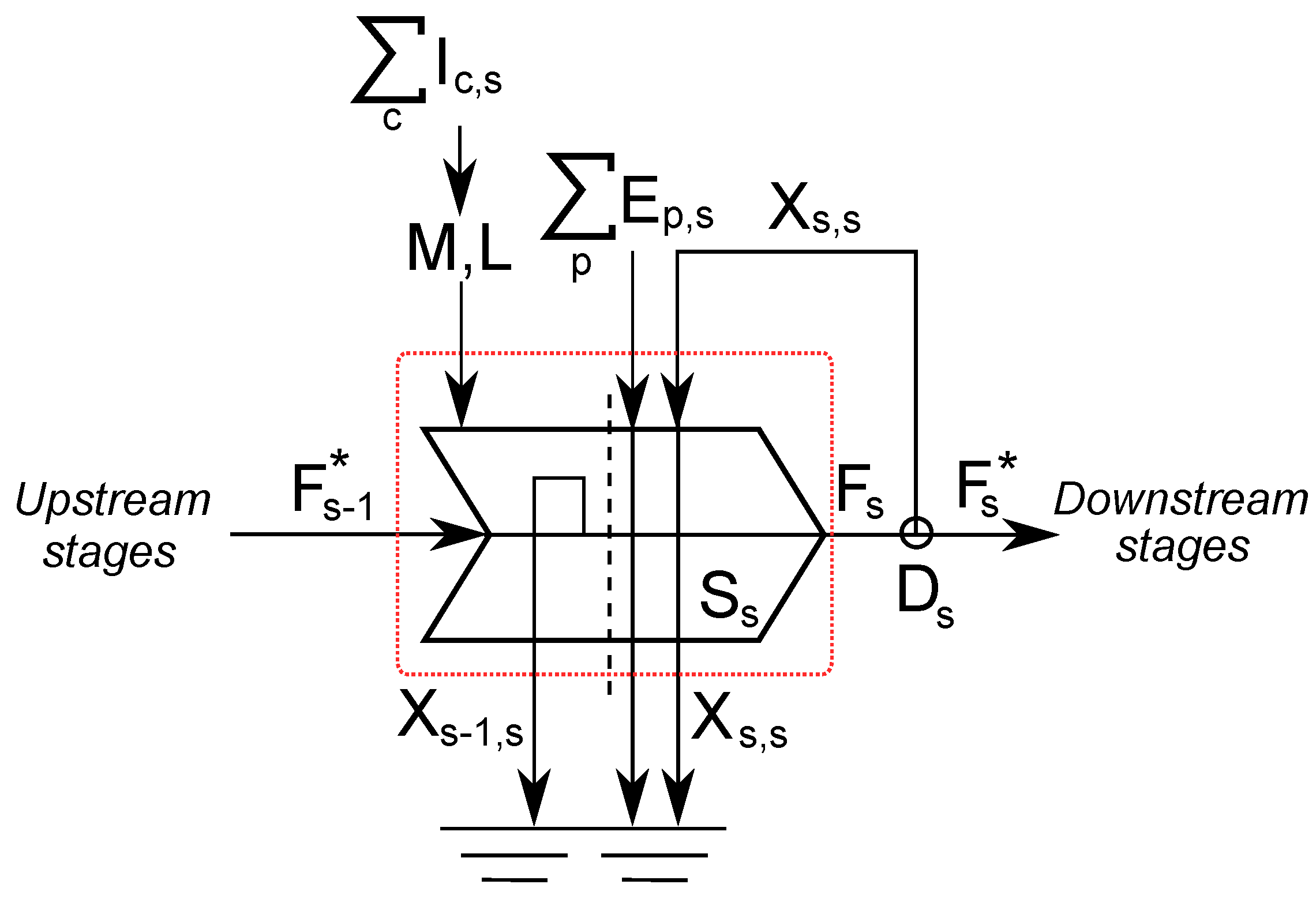
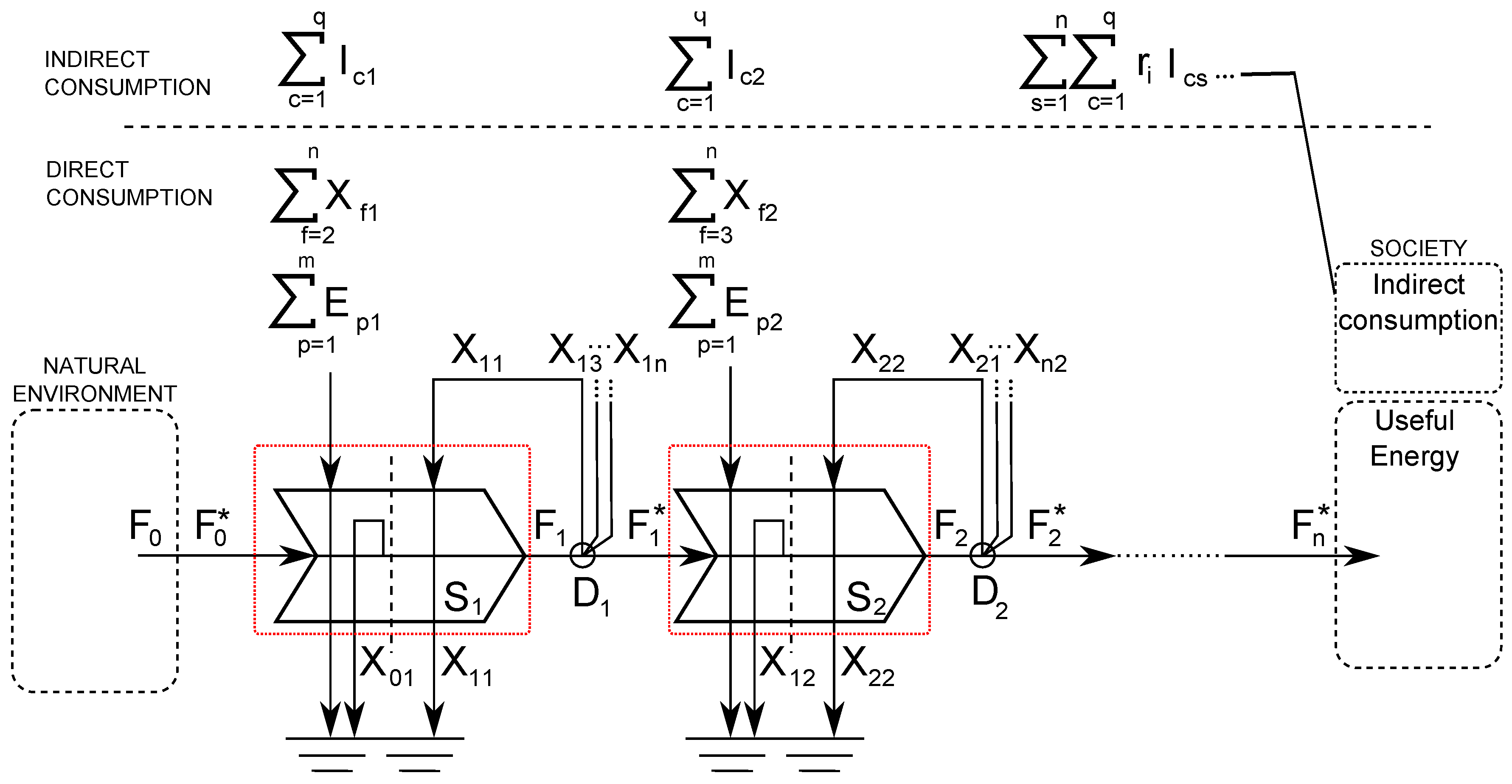
3.1. Types of Processing Stages

A processing stage in our model is a general term for any technology (or functionally grouped set of technologies) that transforms the principal energy flow through it. Our model recognizes five fundamental transformations that can be performed on a principal energy flow:

• Harvesting, capturing, or gathering of the primary energy carrier (the initial form of the principal energy flow) from the natural environment. This might include the lifting of crude oil from the subsurface or the conversion of energy contained in photons to electrical energy in a PV panel.
• Shifting energy availability in space. This includes the transport of a principal energy flow from one location in space to another, as in the movement of crude oil from an oil field to a refinery via pipeline or the transport of solar PV electricity from generators to consumers.
• Shifting energy availability in time. This is the shifting of a principal energy flow from one time period to another later time period (storage). Examples include the storage of solar-PV-generated electricity in batteries for use at night, or the storage of crude oil in oil tanks before processing.
• Upgrading or improvement in the quality of a principal energy flow. This is a chemical or physical conversion that does not change the fundamental character of the energy type, but improves its usefulness or quality. An example might be an oil refinery hydrotreating unit that removes sulfur from distillate fuels (e.g., creating ultra-low-sulfur diesel fuel from conventional diesel fuel). Another example might be the transformation of DC solar PV electricity to AC power in an inverter.
• Conversion from one fundamental energy type to another. This is the use of a technology to convert the principal energy flow from one physical form to another. This is typically a more profound and fundamental change than upgrading the principal energy flow. For example, this might involve the conversion from chemical potential energy in gasoline (which exists due to hydrocarbons being out of equilibrium with an oxygen-rich atmosphere) to rotational kinetic energy using a heat engine.

The scale of a processing stage is not specified in our model. Depending on the level of aggregation desired, a processing stage could be as complex as transport of electrons on a region-wide electricity grid, or as simple as a single inverter that converts DC power from a solar panel into grid-ready AC current. Some processing stages are multi-functional (e.g., an oil pipeline transports oil in both time and space) and therefore ambiguity can exist in trying to strictly classify a processing stage.

3.1.1. Example of a Processing Stage

Our framework for a processing stage is illustrated in Figure 1. Into the processing stage boundary (in this case for processing stage s) flows principal energy flow $F_{s-1}^{*}$. This is the flow of energy from the previous process stage (stage $s-1$) after principal energy flow to other stages is subtracted (see below). Within the processing stage boundary, some self-consumption of input primary energy flow (flow $X_{s-1,s}$) can occur in order to fuel the conversion process. At the black dashed line, we assume that the transformation or processing of the principal energy stream occurs. Out of processing stage s flows $F_s$, the altered principal energy flow (again, this transformation can be refining, upgrading, storing, transporting, or otherwise altering the principal energy flow). Some of this altered principal energy flow may be diverted back into the processing stage as flow $X_{s,s}$, reducing the amount of principal energy flow available to the next processing stage or to final consumption.

Figure 1. Schematic for flows within a single processing stage.

Figure 1. Schematic for flows within a single processing stage.

Note that the notation for self-consumption (X) flows records the principal flow type consumed, followed by the index for the flow type created. Alternatively, since flow $F_{s-1}$ can be thought of as the flow from the stage from which the principal energy flow arrived, and s is the stage into which the energy flows, the notation can be thought of as $X_{s-1,s}=X_{f,t}=X_{from,to}$. In the first stage of a processing chain ($s=1$) the principal energy flow is $F_0^{*}$ and any self-consumed raw energy from the environment is treated as flow $X_{01}$.

Using oil refining as a processing stage example, the refinery might take in crude oil ($F_{s-1}$), consume some of the energy in the crude oil in the process of refining ($X_{s-1,s}$) in order to generate a variety of refined products ($F_s$). If some of these finished products are fed back into the process, such as diesel fuel used in trucks on site at the refinery, then this would be labeled as self-consumption of finished product ($X_{s,s}$).

Note that our model assumes that consumption of finished energy occurs outside of the process boundary (i.e., $X_{s,s}$ flows out of the process as part of $F_s$ and then back into the process). This formulation is based on the CERI framework [10], which argues that external treatment of self-consumed finished energy is more explicit and avoids concealing energy consumption within the boundary that could otherwise be exported as finished energy (in principle, if not in practice).

After the processing stage s, a distribution point $D_s$ occurs where principal energy can be fed back into the process (or to other up- or down-stream stages) (see small circle). After this distribution point, the net output from the system $F_s^{*}$ can be computed (as compared to gross output $F_s$). These distinctions become important below when comparing net and gross energy return ratios.

In addition to self consumption of the principal energy flow (either before or after conversion), external energy E can be consumed in a processing stage. We draw a distinction between internal energy and external energy as follows: external inputs are derived from an energy extraction and conversion pathway other than the one under consideration, while internal energy inputs come from within the same pathway, even if they come from another stage in the pathway. External energy inputs E are indexed by the pathway that generated the external energy ($p=1,\dots ,m$) and the processing stage in which they are consumed (in this figure, stage s).

For example, an oil refinery might consume external energy in the form of electricity generated with multiple fuels (e.g., natural gas and coal-fired electricity), or as natural gas for hydrogen production (so $m=3$). Energy consumed that is generated downstream in the same pathway (e.g., gasoline consumed on site at the refinery) would be counted as an internal energy input X [41].

Also, in order to count all energy consumed by a processing stage, indirect energy use must be counted as well. This indirect consumption occurs outside of the system boundary of the process and is required to supply external energy (E), labor (L), and materials used directly (M) within the energy processing stage. These myriad indirect energy inputs are signified with I, indexed by the economic sector c in which the consumption occurs. These inputs therefore represent “embodied” energy within external energy and materials consumed in the processing stages.

The indirect use term I illustrates the requirement for consistent and well-defined system boundaries for processes. In our formulation, the system boundary for a process is a temporal and spatial boundary that separates the process from its surroundings (things that are not the process). Across this system boundary a variety of consumptive flows occur: energy can flow in to be consumed (internal and external energy), human labor and ingenuity are consumed, and materials are consumed in a consumptive fashion or for capital investment. Each of these flows can be associated with some energy consumption that occurs outside of the process boundary.

For example, a specialist consultant might work intermittently at an oil refinery. Any overhead energy required to support his professional practice could be allocated to the refinery as indirect energy consumption in proportion to the fraction of his services that it consumes (e.g., lighting and computer use in an off-site office). In contrast, electricity used on site by this consultant would be a direct energy consumptive activity, either an internal energy consumption (if it were co-generated on site using petroleum residues such as process gas) or an external energy consumption (if it comes from the wider grid).

Calculating indirect energy inputs comprehensively and accurately is difficult. Economic input-output (EIO) based life cycle assessment (EIO-LCA) has been used to track these direct and indirect consumptive factors [38]. Including this indirect consumption expands our model system boundaries from being a purely “bottom-up” process model to a “hybrid” process-EIO model, or a hybrid EROI calculation.

Returning to the example of an oil refinery, externally-purchased natural gas is often consumed in oil refining. EIO-LCA data suggest that consuming 1 MJ of natural gas directly results in approximate total lifecycle consumption (in all sectors of the economy) of 0.03 MJ coal, 1.04 MJ of natural gas, 0.01 MJ petroleum, 0.00 MJ of biomass and waste energy, and 0.01 MJ of non-fossil electricity [42]. Therefore, summing all of these coefficients results in an effective 0.08 MJ consumed indirectly per MJ of direct natural gas energy consumed [43]. In this model formulation, we assume that all external energy types are equivalent for simplicity—all energy types are summed using simple thermal equivalents [44].

Figure 2. Observed flows in US refining sector, 2008 [45], neglecting indirect (embodied) consumption. Deviation from our simple model occurs due to the inclusion of some energy content from external natural gas inputs into the principal energy stream in the form of H${}_2$ (called flow $dE$ in this figure). This flow exists in reality but is not included in our simple model of a processing stage. Flows are rounded independently and may not sum exactly to 100. Flow $X_{11}$ is of uncertain magnitude (refined products use within refinery process boundary, e.g., diesel fuel use on refinery site).

Figure 2. Observed flows in US refining sector, 2008 [45], neglecting indirect (embodied) consumption. Deviation from our simple model occurs due to the inclusion of some energy content from external natural gas inputs into the principal energy stream in the form of H${}_2$ (called flow $dE$ in this figure). This flow exists in reality but is not included in our simple model of a processing stage. Flows are rounded independently and may not sum exactly to 100. Flow $X_{11}$ is of uncertain magnitude (refined products use within refinery process boundary, e.g., diesel fuel use on refinery site).

The addition of indirect consumption in our processing stage inputs shifts our boundaries toward that of the life cycle efficiency, as defined by Denholm [46]. The life cycle efficiency of a given process is equal to the conventional efficiency, with additional allowance made for energy consumed indirectly in the life cycle of a process. For example, a combined cycle gas turbine used for power generation might have a rated efficiency of 50% on an LHV basis, while if you add in the energy costs of capital (e.g., steel, cement), materials inputs (repairs and maintenance), and other indirect inputs (e.g., fuel to transport maintenance crews to the turbine) then the life cycle efficiency might decline to, say, 48%.

As an example processing stage, energy flows for the US oil refining sector are shown in Figure 2. Note that this real-world case does not align exactly with our model: there is a flow $dE$ in the model that incorporates external energy in the form of natural gas into the principal energy flow.

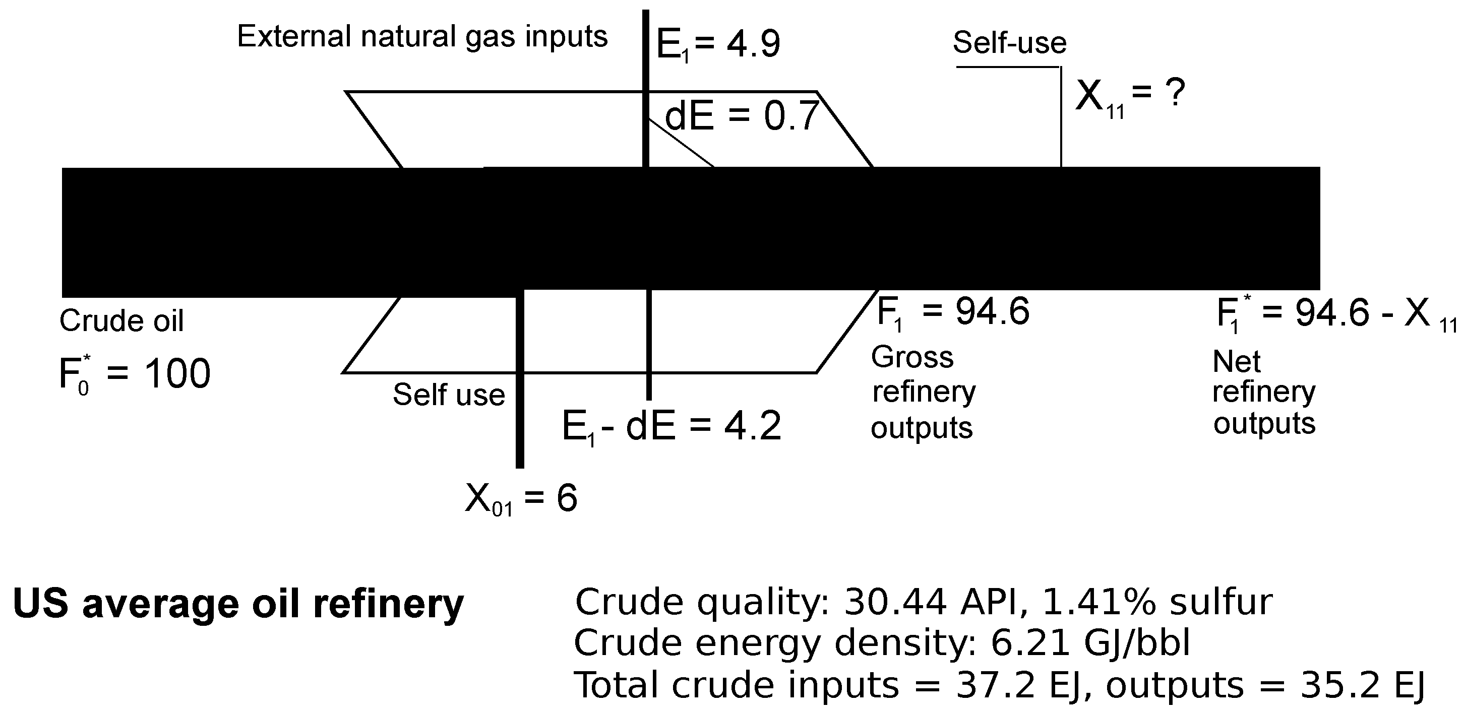
3.1.2. Processing Stage Efficiency

The efficiency of a processing stage can be defined in numerous ways. We define a number of efficiencies in order to usefully recast the ERRs defined below as functions of normalized process efficiency. Each efficiency is created by applying a consistent system boundary to a process with some subset of the flows included in the process (see appendix for derivation). By their nature, they are all equal to or less than 1 (less useful energy leaves a process than comes into the process). The simplest of these efficiencies neglects all of the “outside of boundary” inputs shown above, while the most comprehensive includes all direct and indirect inputs.

The most basic efficiency, called the flow-through efficiency, or ${\eta }^{\alpha }$ neglects all consumption that originates outside of the process boundary. For stage number 1 ($s=1$), ${\eta }^{\alpha }$ is defined as:

$${\eta }_1^{\alpha }=\frac{F_1}{F_0^{*}}$$

(1)

${\eta }^{\alpha }$ represents the fraction of the input energy $F_0$ that leaves as useful output energy $F_1$ after losses and self consumption (X) are subtracted [47]. It is also useful to define a second efficiency ${\eta }^{\beta }$, also called the consumptive efficiency:

$${\eta }_1^{\beta }=\frac{F_1}{F_0^{*}+{\displaystyle \sum _{f=1}^n}{X}_{f1}}$$

(2)

${\eta }^{\beta }$ is a broader metric, as it includes in the denominator the within-pathway energy consumed in the process as well as the primary energy input. Here n represents the total number of stages in the pathway (see below for discussion of energy extraction and conversion pathways).

Next, we can generalize the efficiency further to include direct consumption of external energy (therefore called the external efficiency) ${\eta }^{\gamma }$:

$${\eta }_1^{\gamma }=\frac{F_1}{F_0^{*}+{\displaystyle \sum _{f=1}^n}{X}_{f1}+{\displaystyle \sum _{p=1}^m}{E}_{p1}}$$

(3)

This external efficiency corresponds to what can be considered a gross stage efficiency: it represents total useful energy output divided by total useful energy inputs. For example, this might represent the total outputs of refined product from a refinery (before any self-consumption of refined product in the refinery is subtracted) divided by the total internal and external energy consumed in refining. As noted above, for simplicity we assume that all $E_p$ leave the stage as waste energy (i.e., are consumed) and none are incorporated into the primary energy stream.

Lastly, we generate the life cycle efficiency ${\eta }^{\delta }$, which is the most general efficiency metric for a process in that it also includes indirect consumption of energy:

$${\eta }_1^{\delta }=\frac{F_1}{F_0^{*}+{\displaystyle \sum _{f=1}^n}{X}_{f1}+{\displaystyle \sum _{p=1}^m}{E}_{p1}+{\displaystyle \sum _{c=1}^q}{I}_{c1}}$$

(4)

where in this case we include the term I for indirect consumption that occurs outside of the immediate location of the energy processing stage. The use of these efficiencies to derive efficiency-based ERRs is outlined in detail in the appendix.

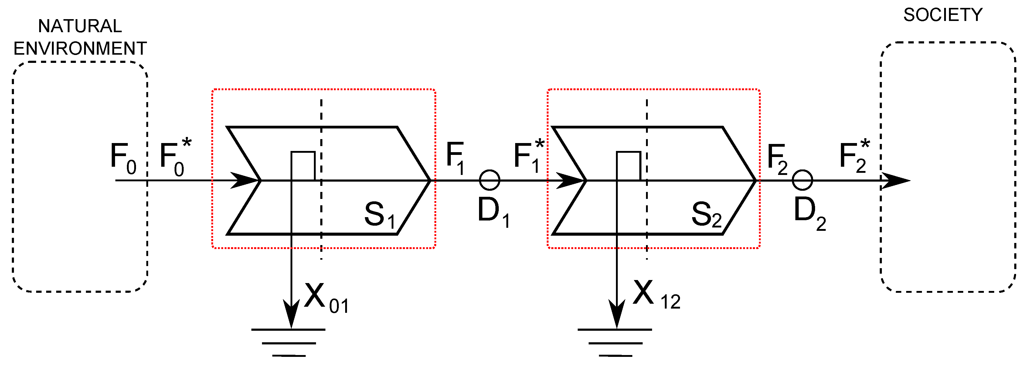
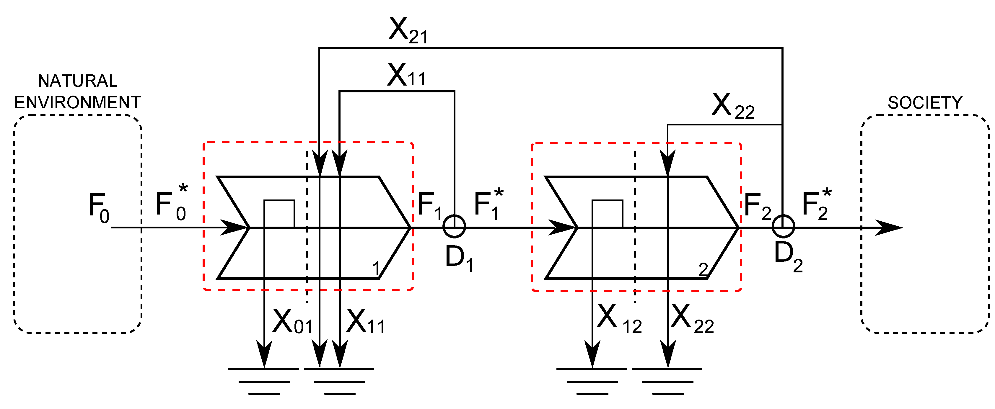
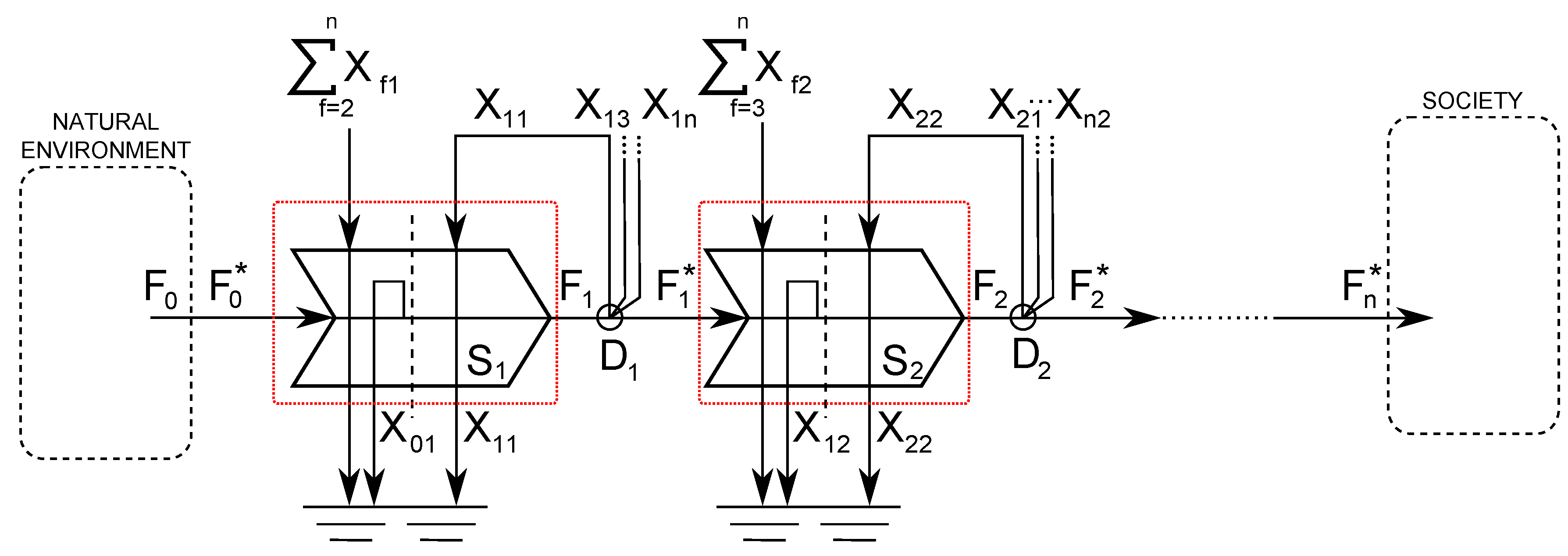
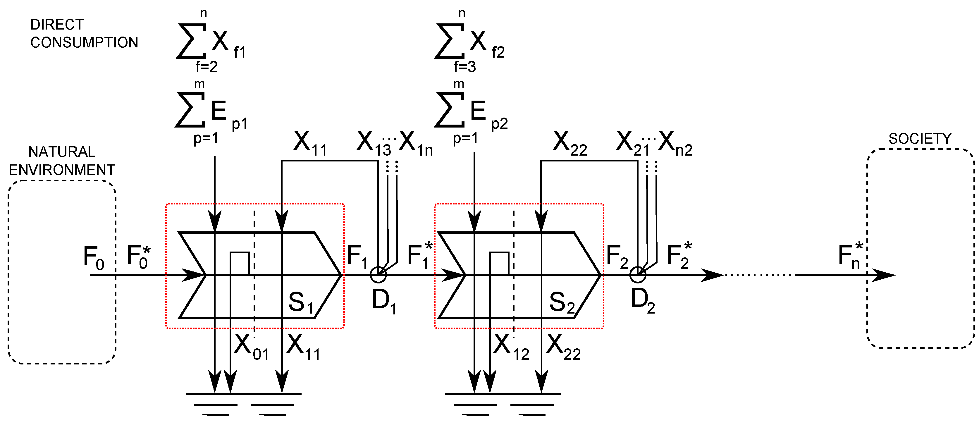
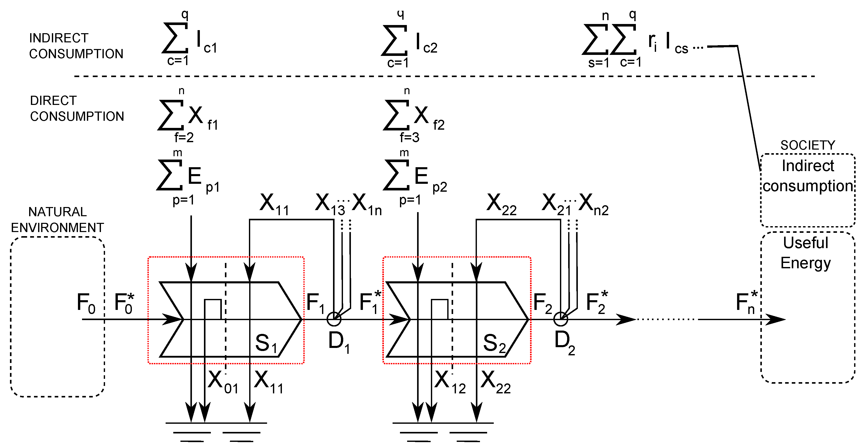
3.2. Energy Pathway Analysis

Using the above concept of a processing stage, energy extraction and conversion pathways (P) can be generated by chaining together a variety of stages (labeled $S_1\dots S_n$). A schematic n-stage model is illustrated in Figure 3. As the figure shows, an energy extraction and conversion pathway can be defined as a series of processing stages of varying characteristics, efficiencies and functions. Depending on the extent of data disaggregation, a pathway can include arbitrary numbers of processing stages, and each processing stage can be of varying complexity (e.g., an entire sector or a single device).

Figure 3. Energy production process with one pathway and n stages.

Figure 3. Energy production process with one pathway and n stages.

In between each processing stage a point of principal energy distribution (distribution point $D_1\dots D_n$) exists, which consumes no energy but serves as the point where the principal energy stream can be diverted to other stages. Energy is conserved across process boundaries and across distribution point boundaries (see appendix). Each distribution point is subject to its own pass-through ratio φ:

$${\varphi }_s=\frac{F_s^{*}}{F_s}$$

(5)

By tracking energy balances across each processing stage, the following information can be obtained:

• The flow of principal energy type $F_s$ leaving a given processing stage s;
• The total self consumption inputs to a stage s from all other stages within the pathway (${\displaystyle \sum _f}{X}_{fs}$);
• The total external inputs to a stage s from all external energy types (adjusted for indirect consumption, ${\displaystyle \sum _p}{E}_{ps}$);
• The total embodied energy induced in all economic sectors c due to external energy and materials consumed in stage s (${\displaystyle \sum _c}{I}_{cs}$).

These results can be summed across stages ($s=1,\dots ,n$) and compared to the output from the process in order to calculate ERRs.

We generate mathematical formulations for 4 ERRs below, including the net energy return (NER), the gross energy return (GER), the net external energy return (NEER) and the gross external energy return (GEER) [1,13].

The NER is the ratio of net outputs to society to the total amount of energy consumed in production [48]. In contrast, the GER uses the gross output from the final processing stage (before any self consumption of the final product is removed). The NEER is computed as the net final energy provided by a process, divided by the energy input to the process from only the external energy system, and the GEER computes the same but for gross energy output. NEER and GEER are indicators of the ability of a process to increase the energy supply to society [49].

These ERRs vary due to (a) the nature of the numerator (gross or net output); (b) the system boundary applied to the numerator (e.g., output of refined energy or output of raw energy from extraction); (c) the system boundary applied to the denominator; (d) the inclusion of all energy inputs in the denominator or inclusion of only external inputs; and (e) the specification of the ERR in terms of flow-based or efficiency-based variables.

First, ERRs can vary in whether they count gross or net output from the processing chain as the relevant output metric. For example, the GER for an oil pathway would count all energy products from a refinery as gross output, while an NER would subtract out all “backward” flows of refined oil products back into the process chain (e.g., diesel fuel consumed in drill rigs).

Second, ERRs can vary in whether they include downstream processing stages in the equation. That is, does the system boundary include further processing, or does it only include extraction? Some EROI calculations use “mine-mouth” system boundaries, where only raw extraction from the environment is included, while others include downstream processing. Our models focus on calculations that include all processing stages until an energy product ready to be used in society is produced.

Third, the system boundary applied to the pathway can be tightly-circumscribed, with internal self-consumption only, or very broad, with indirect energy use throughout the economy calculated using a hybrid-EIO approach. Our formulation below shows ERRs for three possible system boundaries, corresponding to the processing stage efficiencies presented above: consumptive ERRs include only self-use, representing the most restrictive system boundary; external ERRs add the direct consumption of external energy types; and life cycle ERRs add indirect consumption due to external energy consumption and embodied energy in materials.

Fourth, the denominator can vary depending on whether or not it counts internal (self) consumption as part of the production process input energy. An ERR can include all energy inputs to the process, which generates the NER or GER. Alternatively, if only external inputs are included (that is, internal energy inputs are ignored) then the NEER or GEER is calculated.

Lastly, ERRs can be specified using flow-based or efficiency-based variables. If the ERR is specified using absolute magnitudes of flows (such as $F_s$ and $X_{ft}$), we call this a flow-based ERR. If, in contrast, the efficiencies of processing stages (such as ${\eta }^{\alpha }$ and ${\eta }^{\beta }$) are used, then an efficiency-based ERR is calculated. ERRs calculated using flow-based and efficiency-based frameworks are mathematically equivalent, and differ only in the required data inputs. If magnitudes of energy throughput are available, then the flow-based ratios will be more useful, while if technology efficiencies are available, then efficiency-based metrics are more useful.

Using the above framework, n-stage models are generated for both flow-based and efficiency-based formulations. Formulations for NER and GER are presented in Table 1, while NEER and GEER are presented in Table 2. The flow-based and efficiency-based variables used in these formulations are defined in Table 3. The attached appendix gives a full derivation of the models, including derivation of simpler two-stage pathways used to explain the logic of the n-stage ratios.

A key feature of life cycle ERRs is the reduction of the numerator (output energy) by some amount of indirect consumption of the principal energy stream (${\displaystyle \sum _c}{\displaystyle \sum _s}{r}_i{I}_{cs}$). In any pathway, p, ERRs calculated using life cycle system boundaries must exclude the amount of principal energy from $F_n$ that is consumed (indirectly) in the production of external energy and materials consumed in pathway p. To develop these estimates, a hybrid process-EIO can be used (our model uses a single economy-wide factor for simplicity).

Again using the example of an oil refinery, consuming external natural gas in an oil refinery adds consumption to the denominator of the NER not only directly (through on-site consumption of natural gas) but also indirectly through upstream off-site consumption required to supply natural gas to the production process. Any indirect consumption of our principal energy flow (oil) due to the natural gas life cycle must be subtracted from the numerator. That is, some amount of finished oil product is consumed to supply external natural gas to the refinery processing stage (such as diesel fuel consumed in natural gas drilling rigs). This indirect self use lessens the net output of oil products to the rest of society from the oil extraction and processing pathway.

Most applications of EROI analysis in the literature aim for the life cycle flow-based GER (or NER in some cases), although often the method of computing EROI is not explicitly defined. We therefore include the EROI under the life cycle GER heading and consider the other forms of GER to be variants of EROI with different system boundaries [50].

Table 1. NER and GER formulations based on flows of energy (flow-based) and process stage efficiencies (efficiency-based). The EROI as generally practiced would fall under the heading of a life-cycle based GER.

ERR Type	Net Energy Return (NER)	Gross Energy Return (GER)
Consumptive (Flow)	${\displaystyle NE{R}_n^{\beta }=\frac{F_n^{*}}{X_{01}+{\displaystyle \sum _f}{\displaystyle \sum _t}{X}_{ft}}}$	${\displaystyle GE{R}_n^{\beta }=\frac{F_n}{X_{01}+{\displaystyle \sum _f}{\displaystyle \sum _t}{X}_{ft}}}$
Consumptive (Efficiency)	${\displaystyle NE{R}_n^{\beta }=\frac{{\displaystyle \prod _{s=1}^n}{\varphi }_s{\eta }_s^{\alpha }}{{\displaystyle \prod _{s=1}^1}{\varphi }_{s-1}{\eta }_s^{\alpha }\left(\frac{1}{{\eta }_1^{\beta }}-1\right)+\cdots +{\displaystyle \prod _{s=1}^n}{\varphi }_{s-1}{\eta }_s^{\alpha }\left(\frac{1}{{\eta }_n^{\beta }}-1\right)}}$	${\displaystyle GE{R}_n^{\beta }=\frac{{\displaystyle \prod _{s=1}^n}{\varphi }_{s-1}{\eta }_s^{\alpha }}{{\displaystyle \prod _{s=1}^1}{\varphi }_{s-1}{\eta }_s^{\alpha }\left(\frac{1}{{\eta }_1^{\beta }}-1\right)+\cdots +{\displaystyle \prod _{s=1}^n}{\varphi }_{s-1}{\eta }_s^{\alpha }\left(\frac{1}{{\eta }_n^{\beta }}-1\right)}}$
External (Flow)	${\displaystyle NE{R}_n^{\gamma }=\frac{F_n^{*}}{X_{01}+{\displaystyle \sum _f}{\displaystyle \sum _t}{X}_{ft}+{\displaystyle \sum _p}{\displaystyle \sum _s}{E}_{ps}}}$	${\displaystyle GE{R}_n^{\gamma }=\frac{F_n}{X_{01}+{\displaystyle \sum _f}{\displaystyle \sum _t}{X}_{ft}+{\displaystyle \sum _p}{\displaystyle \sum _s}{E}_{ps}}}$
External (Efficiency)	${\displaystyle NE{R}_n^{\gamma }=\frac{{\displaystyle \prod _{s=1}^n}{\varphi }_s{\eta }_s^{\alpha }}{{\displaystyle \prod _{s=1}^1}{\varphi }_{s-1}{\eta }_s^{\alpha }\left(\frac{1}{{\eta }_1^{\gamma }}-1\right)+\cdots +{\displaystyle \prod _{s=1}^n}{\varphi }_{s-1}{\eta }_s^{\alpha }\left(\frac{1}{{\eta }_n^{\gamma }}-1\right)}}$	${\displaystyle GE{R}_n^{\gamma }=\frac{{\displaystyle \prod _{s=1}^n}{\varphi }_{s-1}{\eta }_s^{\alpha }}{{\displaystyle \prod _{s=1}^1}{\varphi }_{s-1}{\eta }_s^{\alpha }\left(\frac{1}{{\eta }_1^{\gamma }}-1\right)+\cdots +{\displaystyle \prod _{s=1}^n}{\varphi }_{s-1}{\eta }_s^{\alpha }\left(\frac{1}{{\eta }_n^{\gamma }}-1\right)}}$
Life cycle (Flow) [EROI]	${\displaystyle NE{R}_n^{\delta }=\frac{F_n^{*}-r_i{\displaystyle \sum _c}{\displaystyle \sum _s}{I}_{cs}}{X_{01}+{\displaystyle \sum _f}{\displaystyle \sum _t}{X}_{ft}+{\displaystyle \sum _p}{\displaystyle \sum _s}{E}_{ps}+{\displaystyle \sum _c}{\displaystyle \sum _s}{I}_{cs}}}$	${\displaystyle GE{R}_n^{\delta }=\frac{F_n}{X_{01}+{\displaystyle \sum _f}{\displaystyle \sum _t}{X}_{ft}+{\displaystyle \sum _p}{\displaystyle \sum _s}{E}_{ps}+{\displaystyle \sum _c}{\displaystyle \sum _s}{I}_{cs}}}$
Life cycle (Efficiency)	${\displaystyle NE{R}_n^{\delta }=\frac{{\displaystyle \prod _{s=1}^n}{\varphi }_s{\eta }_s^{\alpha }-r_i{\displaystyle \sum _{j=1}^n}\left[{\displaystyle \prod _{s=1}^j}{\varphi }_{s-1}{\eta }_s^{\alpha }\left(\frac{1}{{\eta }_j^{\delta }}-\frac{1}{{\eta }_j^{\gamma }}\right)\right]}{{\displaystyle \prod _{s=1}^1}{\varphi }_{s-1}{\eta }_s^{\alpha }\left(\frac{1}{{\eta }_1^{\delta }}-1\right)+\cdots +{\displaystyle \prod _{s=1}^n}{\varphi }_{s-1}{\eta }_s^{\alpha }\left(\frac{1}{{\eta }_n^{\delta }}-1\right)}}$	${\displaystyle GE{R}_n^{\delta }=\frac{{\displaystyle \prod _{s=1}^n}{\varphi }_{s-1}{\eta }_s^{\alpha }}{{\displaystyle \prod _{s=1}^1}{\varphi }_{s-1}{\eta }_s^{\alpha }\left(\frac{1}{{\eta }_1^{\delta }}-1\right)+\cdots +{\displaystyle \prod _{s=1}^n}{\varphi }_{s-1}{\eta }_s^{\alpha }\left(\frac{1}{{\eta }_n^{\delta }}-1\right)}}$

Table 1. NER and GER formulations based on flows of energy (flow-based) and process stage efficiencies (efficiency-based). The EROI as generally practiced would fall under the heading of a life-cycle based GER.

ERR Type	Net Energy Return (NER)	Gross Energy Return (GER)
Consumptive (Flow)	${\displaystyle NE{R}_n^{\beta }=\frac{F_n^{*}}{X_{01}+{\displaystyle \sum _f}{\displaystyle \sum _t}{X}_{ft}}}$	${\displaystyle GE{R}_n^{\beta }=\frac{F_n}{X_{01}+{\displaystyle \sum _f}{\displaystyle \sum _t}{X}_{ft}}}$
Consumptive (Efficiency)	${\displaystyle NE{R}_n^{\beta }=\frac{{\displaystyle \prod _{s=1}^n}{\varphi }_s{\eta }_s^{\alpha }}{{\displaystyle \prod _{s=1}^1}{\varphi }_{s-1}{\eta }_s^{\alpha }\left(\frac{1}{{\eta }_1^{\beta }}-1\right)+\cdots +{\displaystyle \prod _{s=1}^n}{\varphi }_{s-1}{\eta }_s^{\alpha }\left(\frac{1}{{\eta }_n^{\beta }}-1\right)}}$	${\displaystyle GE{R}_n^{\beta }=\frac{{\displaystyle \prod _{s=1}^n}{\varphi }_{s-1}{\eta }_s^{\alpha }}{{\displaystyle \prod _{s=1}^1}{\varphi }_{s-1}{\eta }_s^{\alpha }\left(\frac{1}{{\eta }_1^{\beta }}-1\right)+\cdots +{\displaystyle \prod _{s=1}^n}{\varphi }_{s-1}{\eta }_s^{\alpha }\left(\frac{1}{{\eta }_n^{\beta }}-1\right)}}$
External (Flow)	${\displaystyle NE{R}_n^{\gamma }=\frac{F_n^{*}}{X_{01}+{\displaystyle \sum _f}{\displaystyle \sum _t}{X}_{ft}+{\displaystyle \sum _p}{\displaystyle \sum _s}{E}_{ps}}}$	${\displaystyle GE{R}_n^{\gamma }=\frac{F_n}{X_{01}+{\displaystyle \sum _f}{\displaystyle \sum _t}{X}_{ft}+{\displaystyle \sum _p}{\displaystyle \sum _s}{E}_{ps}}}$
External (Efficiency)	${\displaystyle NE{R}_n^{\gamma }=\frac{{\displaystyle \prod _{s=1}^n}{\varphi }_s{\eta }_s^{\alpha }}{{\displaystyle \prod _{s=1}^1}{\varphi }_{s-1}{\eta }_s^{\alpha }\left(\frac{1}{{\eta }_1^{\gamma }}-1\right)+\cdots +{\displaystyle \prod _{s=1}^n}{\varphi }_{s-1}{\eta }_s^{\alpha }\left(\frac{1}{{\eta }_n^{\gamma }}-1\right)}}$	${\displaystyle GE{R}_n^{\gamma }=\frac{{\displaystyle \prod _{s=1}^n}{\varphi }_{s-1}{\eta }_s^{\alpha }}{{\displaystyle \prod _{s=1}^1}{\varphi }_{s-1}{\eta }_s^{\alpha }\left(\frac{1}{{\eta }_1^{\gamma }}-1\right)+\cdots +{\displaystyle \prod _{s=1}^n}{\varphi }_{s-1}{\eta }_s^{\alpha }\left(\frac{1}{{\eta }_n^{\gamma }}-1\right)}}$
Life cycle (Flow) [EROI]	${\displaystyle NE{R}_n^{\delta }=\frac{F_n^{*}-r_i{\displaystyle \sum _c}{\displaystyle \sum _s}{I}_{cs}}{X_{01}+{\displaystyle \sum _f}{\displaystyle \sum _t}{X}_{ft}+{\displaystyle \sum _p}{\displaystyle \sum _s}{E}_{ps}+{\displaystyle \sum _c}{\displaystyle \sum _s}{I}_{cs}}}$	${\displaystyle GE{R}_n^{\delta }=\frac{F_n}{X_{01}+{\displaystyle \sum _f}{\displaystyle \sum _t}{X}_{ft}+{\displaystyle \sum _p}{\displaystyle \sum _s}{E}_{ps}+{\displaystyle \sum _c}{\displaystyle \sum _s}{I}_{cs}}}$
Life cycle (Efficiency)	${\displaystyle NE{R}_n^{\delta }=\frac{{\displaystyle \prod _{s=1}^n}{\varphi }_s{\eta }_s^{\alpha }-r_i{\displaystyle \sum _{j=1}^n}\left[{\displaystyle \prod _{s=1}^j}{\varphi }_{s-1}{\eta }_s^{\alpha }\left(\frac{1}{{\eta }_j^{\delta }}-\frac{1}{{\eta }_j^{\gamma }}\right)\right]}{{\displaystyle \prod _{s=1}^1}{\varphi }_{s-1}{\eta }_s^{\alpha }\left(\frac{1}{{\eta }_1^{\delta }}-1\right)+\cdots +{\displaystyle \prod _{s=1}^n}{\varphi }_{s-1}{\eta }_s^{\alpha }\left(\frac{1}{{\eta }_n^{\delta }}-1\right)}}$	${\displaystyle GE{R}_n^{\delta }=\frac{{\displaystyle \prod _{s=1}^n}{\varphi }_{s-1}{\eta }_s^{\alpha }}{{\displaystyle \prod _{s=1}^1}{\varphi }_{s-1}{\eta }_s^{\alpha }\left(\frac{1}{{\eta }_1^{\delta }}-1\right)+\cdots +{\displaystyle \prod _{s=1}^n}{\varphi }_{s-1}{\eta }_s^{\alpha }\left(\frac{1}{{\eta }_n^{\delta }}-1\right)}}$

Table 2. NEER and GEER formulations based on flows of energy (flow-based) and process stage efficiencies (efficiency-based).

ERR Type	Net External Energy Return (NEER)	Gross External Energy Return (GEER)
Consumptive (Flow)	${\displaystyle NEE{R}_n^{\beta }=\frac{F_n^{*}}{0}=\infty }$	${\displaystyle GEE{R}_n^{\beta }=\frac{F_n}{0}=\infty }$
Consumptive (Efficiency)	${\displaystyle NEE{R}_n^{\beta }=\frac{{\displaystyle \prod _{s=1}^n}{\varphi }_s{\eta }_s^{\alpha }}{0}}$	${\displaystyle GEE{R}_n^{\beta }=\frac{{\displaystyle \prod _{s=1}^n}{\varphi }_{s-1}{\eta }_s^{\alpha }}{0}}$
External (Flow)	${\displaystyle NEE{R}_n^{\gamma }=\frac{F_n^{*}}{{\displaystyle \sum _p}{\displaystyle \sum _s}{E}_{ps}}}$	${\displaystyle GEE{R}_n^{\gamma }=\frac{F_n}{{\displaystyle \sum _p}{\displaystyle \sum _s}{E}_{ps}}}$
External (Efficiency)	${\displaystyle NEE{R}_n^{\beta }=\frac{{\displaystyle \prod _{s=1}^n}{\varphi }_s{\eta }_s^{\alpha }}{{\displaystyle \prod _{s=1}^1}{\varphi }_{s-1}{\eta }_s^{\alpha }\left(\frac{1}{{\eta }_1^{\gamma }}-\frac{1}{{\eta }_1^{\beta }}\right)+\cdots +{\displaystyle \prod _{s=1}^n}{\varphi }_{s-1}{\eta }_s^{\alpha }\left(\frac{1}{{\eta }_n^{\gamma }}-\frac{1}{{\eta }_n^{\beta }}\right)}}$	${\displaystyle GEE{R}_n^{\beta }=\frac{{\displaystyle \prod _{s=1}^n}{\varphi }_{s-1}{\eta }_s^{\alpha }}{{\displaystyle \prod _{s=1}^1}{\varphi }_{s-1}{\eta }_s^{\alpha }\left(\frac{1}{{\eta }_1^{\gamma }}-\frac{1}{{\eta }_1^{\beta }}\right)+\cdots +{\displaystyle \prod _{s=1}^n}{\varphi }_{s-1}{\eta }_s^{\alpha }\left(\frac{1}{{\eta }_n^{\gamma }}-\frac{1}{{\eta }_n^{\beta }}\right)}}$
Life cycle (Flow) [EROI]	${\displaystyle NEE{R}_n^{\delta }=\frac{F_n^{*}-r_i{\displaystyle \sum _c}{\displaystyle \sum _s}{I}_{cs}}{{\displaystyle \sum _p}{\displaystyle \sum _s}{E}_{ps}+{\displaystyle \sum _c}{\displaystyle \sum _s}{I}_{cs}}}$	${\displaystyle GEE{R}_n^{\delta }=\frac{F_n}{{\displaystyle \sum _p}{\displaystyle \sum _s}{E}_{ps}+{\displaystyle \sum _c}{\displaystyle \sum _s}{I}_{cs}}}$
Life cycle (Efficiency)	${\displaystyle NEE{R}_n^{\beta }=\frac{{\displaystyle \prod _{s=1}^n}{\varphi }_s{\eta }_s^{\alpha }-r_i{\displaystyle \sum _{j=1}^n}\left[{\displaystyle \prod _{s=1}^j}{\varphi }_{s-1}{\eta }_s^{\alpha }\left(\frac{1}{{\eta }_j^{\delta }}-\frac{1}{{\eta }_j^{\gamma }}\right)\right]}{{\displaystyle \prod _{s=1}^1}{\varphi }_{s-1}{\eta }_s^{\alpha }\left(\frac{1}{{\eta }_1^{\delta }}-\frac{1}{{\eta }_1^{\beta }}\right)+\cdots +{\displaystyle \prod _{s=1}^n}{\varphi }_{s-1}{\eta }_s^{\alpha }\left(\frac{1}{{\eta }_n^{\delta }}-\frac{1}{{\eta }_n^{\beta }}\right)}}$	${\displaystyle GEE{R}_n^{\beta }=\frac{{\displaystyle \prod _{s=1}^n}{\varphi }_{s-1}{\eta }_s^{\alpha }}{{\displaystyle \prod _{s=1}^1}{\varphi }_{s-1}{\eta }_s^{\alpha }\left(\frac{1}{{\eta }_1^{\delta }}-\frac{1}{{\eta }_1^{\beta }}\right)+\cdots +{\displaystyle \prod _{s=1}^n}{\varphi }_{s-1}{\eta }_s^{\alpha }\left(\frac{1}{{\eta }_n^{\delta }}-\frac{1}{{\eta }_n^{\beta }}\right)}}$

Table 2. NEER and GEER formulations based on flows of energy (flow-based) and process stage efficiencies (efficiency-based).

ERR Type	Net External Energy Return (NEER)	Gross External Energy Return (GEER)
Consumptive (Flow)	${\displaystyle NEE{R}_n^{\beta }=\frac{F_n^{*}}{0}=\infty }$	${\displaystyle GEE{R}_n^{\beta }=\frac{F_n}{0}=\infty }$
Consumptive (Efficiency)	${\displaystyle NEE{R}_n^{\beta }=\frac{{\displaystyle \prod _{s=1}^n}{\varphi }_s{\eta }_s^{\alpha }}{0}}$	${\displaystyle GEE{R}_n^{\beta }=\frac{{\displaystyle \prod _{s=1}^n}{\varphi }_{s-1}{\eta }_s^{\alpha }}{0}}$
External (Flow)	${\displaystyle NEE{R}_n^{\gamma }=\frac{F_n^{*}}{{\displaystyle \sum _p}{\displaystyle \sum _s}{E}_{ps}}}$	${\displaystyle GEE{R}_n^{\gamma }=\frac{F_n}{{\displaystyle \sum _p}{\displaystyle \sum _s}{E}_{ps}}}$
External (Efficiency)	${\displaystyle NEE{R}_n^{\beta }=\frac{{\displaystyle \prod _{s=1}^n}{\varphi }_s{\eta }_s^{\alpha }}{{\displaystyle \prod _{s=1}^1}{\varphi }_{s-1}{\eta }_s^{\alpha }\left(\frac{1}{{\eta }_1^{\gamma }}-\frac{1}{{\eta }_1^{\beta }}\right)+\cdots +{\displaystyle \prod _{s=1}^n}{\varphi }_{s-1}{\eta }_s^{\alpha }\left(\frac{1}{{\eta }_n^{\gamma }}-\frac{1}{{\eta }_n^{\beta }}\right)}}$	${\displaystyle GEE{R}_n^{\beta }=\frac{{\displaystyle \prod _{s=1}^n}{\varphi }_{s-1}{\eta }_s^{\alpha }}{{\displaystyle \prod _{s=1}^1}{\varphi }_{s-1}{\eta }_s^{\alpha }\left(\frac{1}{{\eta }_1^{\gamma }}-\frac{1}{{\eta }_1^{\beta }}\right)+\cdots +{\displaystyle \prod _{s=1}^n}{\varphi }_{s-1}{\eta }_s^{\alpha }\left(\frac{1}{{\eta }_n^{\gamma }}-\frac{1}{{\eta }_n^{\beta }}\right)}}$
Life cycle (Flow) [EROI]	${\displaystyle NEE{R}_n^{\delta }=\frac{F_n^{*}-r_i{\displaystyle \sum _c}{\displaystyle \sum _s}{I}_{cs}}{{\displaystyle \sum _p}{\displaystyle \sum _s}{E}_{ps}+{\displaystyle \sum _c}{\displaystyle \sum _s}{I}_{cs}}}$	${\displaystyle GEE{R}_n^{\delta }=\frac{F_n}{{\displaystyle \sum _p}{\displaystyle \sum _s}{E}_{ps}+{\displaystyle \sum _c}{\displaystyle \sum _s}{I}_{cs}}}$
Life cycle (Efficiency)	${\displaystyle NEE{R}_n^{\beta }=\frac{{\displaystyle \prod _{s=1}^n}{\varphi }_s{\eta }_s^{\alpha }-r_i{\displaystyle \sum _{j=1}^n}\left[{\displaystyle \prod _{s=1}^j}{\varphi }_{s-1}{\eta }_s^{\alpha }\left(\frac{1}{{\eta }_j^{\delta }}-\frac{1}{{\eta }_j^{\gamma }}\right)\right]}{{\displaystyle \prod _{s=1}^1}{\varphi }_{s-1}{\eta }_s^{\alpha }\left(\frac{1}{{\eta }_1^{\delta }}-\frac{1}{{\eta }_1^{\beta }}\right)+\cdots +{\displaystyle \prod _{s=1}^n}{\varphi }_{s-1}{\eta }_s^{\alpha }\left(\frac{1}{{\eta }_n^{\delta }}-\frac{1}{{\eta }_n^{\beta }}\right)}}$	${\displaystyle GEE{R}_n^{\beta }=\frac{{\displaystyle \prod _{s=1}^n}{\varphi }_{s-1}{\eta }_s^{\alpha }}{{\displaystyle \prod _{s=1}^1}{\varphi }_{s-1}{\eta }_s^{\alpha }\left(\frac{1}{{\eta }_1^{\delta }}-\frac{1}{{\eta }_1^{\beta }}\right)+\cdots +{\displaystyle \prod _{s=1}^n}{\varphi }_{s-1}{\eta }_s^{\alpha }\left(\frac{1}{{\eta }_n^{\delta }}-\frac{1}{{\eta }_n^{\beta }}\right)}}$

Table 3. Definitions of model terms for quantities with magnitudes and dimensionless ratios.

Stages and Flows
Pathways	$P_p$	$P_1,P_2,\dots ,P_m$	m other energy extraction and conversion pathways, with counter index p	Energy extraction and processing pathways
Stages	$S_s$	$S_1,S_2,\dots ,S_n$	n stages counted with counter index s (or $s1,s2$)	Energy extraction and processing stages
Distribution points	$D_s$	$D_1,D_2,\dots ,D_n$	n distribution points counted with counter index s	Energy distribution points for principal energy flows
Flows	$F_s$	$F_1,F_2,\dots ,F_n$	n flows leaving energy extraction and processing stages (counter index s)	Flows of principal energy (MJ of principal energy type s)
Self consumption	$X_{ft}$	$X_{11},X_{12},\dots ,X_{nn}$	$n\times n$ flows leaving energy extraction and processing stage f and going into stage t ($f=1,\dots ,n$, $t=1,\dots ,n$)	Flows of principal energy (MJ of principal energy type f)
External consumption	$E_{ps}$	$E_{11},E_{12},\dots ,E_{mn}$	$m\times n$ flows leaving energy extraction and conversion pathway m into stage s	Flows of principal energy of type m (MJ of principal energy type m)
Indirect consumption	$I_{cs}$	$I_{11},I_{12},\dots ,I_{qn}$	$q\times n$ flows induced in economic sector c due to direct consumption of materials and energy in stage s	Indirect consumption of all energy types in sector c (MJ of all energy types)
Dependent Variables and Efficiencies
Distribution fraction	${\varphi }_s$	${\varphi }_1$, ${\varphi }_2$, …, ${\varphi }_n$	Ratio of outflow $F_s^{*}$ from distribution point s to inflow $F_s$	Dimensionless ratio
Flow efficiency	${\eta }_s^{\alpha }$	${\eta }_1^{\alpha }$, ${\eta }_2^{\alpha }$, …, ${\eta }_n^{\alpha }$	Ratio of outflow $F_s$ from stage s to inflow $F_{s-1}^{*}$	Dimensionless ratio
Consumptive efficiency	${\eta }_s^{\beta }$	${\eta }_1^{\beta }$, ${\eta }_2^{\beta }$, …, ${\eta }_n^{\beta }$	Ratio of outflow $F_{s_2}$ from stage $s_2$ to sum of inflow $F_{s_2-1}^{*}$ and energy consumed from within pathway (${\sum }_{s1}{X}_{s_1{s}_2}$)	Dimensionless ratio
External efficiency	${\eta }_s^{\gamma }$	${\eta }_1^{\gamma }$, ${\eta }_2^{\gamma }$, …, ${\eta }_n^{\gamma }$	Ratio of outflow $F_{s_2}$ from stage $s_2$ to sum of inflow $F_{s_2-1}^{*}$ and energy consumed from within pathway (${\sum }_{s1}{X}_{s_1{s}_2}$) and from outside the pathway (${\sum }_p{E}_{p{s}_2}$)	Dimensionless ratio
Life cycle efficiency	${\eta }_s^{\delta }$	${\eta }_1^{\delta }$, ${\eta }_2^{\delta }$, …, ${\eta }_n^{\delta }$	Ratio of outflow $F_{s_2}$ from stage $s_2$ to sum of inflow $F_{s_2-1}^{*}$ and energy consumed from within pathway (${\sum }_{s1}{X}_{s_1{s}_2}$) and from outside the pathway (${\sum }_p{E}_{p{s}_2}$) as well as indirect consumption in other economic sectors (${\sum }_c{I}_{c{s}_2}$)	Dimensionless ratio
Indirect self-use ratio	$r_i$	–	The fraction of indirect energy consumed that originally arose from the pathway in question. Can be determined using society-wide energy mix or sector-specific energy mixes.	Dimensionless ratio

Table 3. Definitions of model terms for quantities with magnitudes and dimensionless ratios.

Stages and Flows
Pathways	$P_p$	$P_1,P_2,\dots ,P_m$	m other energy extraction and conversion pathways, with counter index p	Energy extraction and processing pathways
Stages	$S_s$	$S_1,S_2,\dots ,S_n$	n stages counted with counter index s (or $s1,s2$)	Energy extraction and processing stages
Distribution points	$D_s$	$D_1,D_2,\dots ,D_n$	n distribution points counted with counter index s	Energy distribution points for principal energy flows
Flows	$F_s$	$F_1,F_2,\dots ,F_n$	n flows leaving energy extraction and processing stages (counter index s)	Flows of principal energy (MJ of principal energy type s)
Self consumption	$X_{ft}$	$X_{11},X_{12},\dots ,X_{nn}$	$n\times n$ flows leaving energy extraction and processing stage f and going into stage t ($f=1,\dots ,n$, $t=1,\dots ,n$)	Flows of principal energy (MJ of principal energy type f)
External consumption	$E_{ps}$	$E_{11},E_{12},\dots ,E_{mn}$	$m\times n$ flows leaving energy extraction and conversion pathway m into stage s	Flows of principal energy of type m (MJ of principal energy type m)
Indirect consumption	$I_{cs}$	$I_{11},I_{12},\dots ,I_{qn}$	$q\times n$ flows induced in economic sector c due to direct consumption of materials and energy in stage s	Indirect consumption of all energy types in sector c (MJ of all energy types)
Dependent Variables and Efficiencies
Distribution fraction	${\varphi }_s$	${\varphi }_1$, ${\varphi }_2$, …, ${\varphi }_n$	Ratio of outflow $F_s^{*}$ from distribution point s to inflow $F_s$	Dimensionless ratio
Flow efficiency	${\eta }_s^{\alpha }$	${\eta }_1^{\alpha }$, ${\eta }_2^{\alpha }$, …, ${\eta }_n^{\alpha }$	Ratio of outflow $F_s$ from stage s to inflow $F_{s-1}^{*}$	Dimensionless ratio
Consumptive efficiency	${\eta }_s^{\beta }$	${\eta }_1^{\beta }$, ${\eta }_2^{\beta }$, …, ${\eta }_n^{\beta }$	Ratio of outflow $F_{s_2}$ from stage $s_2$ to sum of inflow $F_{s_2-1}^{*}$ and energy consumed from within pathway (${\sum }_{s1}{X}_{s_1{s}_2}$)	Dimensionless ratio
External efficiency	${\eta }_s^{\gamma }$	${\eta }_1^{\gamma }$, ${\eta }_2^{\gamma }$, …, ${\eta }_n^{\gamma }$	Ratio of outflow $F_{s_2}$ from stage $s_2$ to sum of inflow $F_{s_2-1}^{*}$ and energy consumed from within pathway (${\sum }_{s1}{X}_{s_1{s}_2}$) and from outside the pathway (${\sum }_p{E}_{p{s}_2}$)	Dimensionless ratio
Life cycle efficiency	${\eta }_s^{\delta }$	${\eta }_1^{\delta }$, ${\eta }_2^{\delta }$, …, ${\eta }_n^{\delta }$	Ratio of outflow $F_{s_2}$ from stage $s_2$ to sum of inflow $F_{s_2-1}^{*}$ and energy consumed from within pathway (${\sum }_{s1}{X}_{s_1{s}_2}$) and from outside the pathway (${\sum }_p{E}_{p{s}_2}$) as well as indirect consumption in other economic sectors (${\sum }_c{I}_{c{s}_2}$)	Dimensionless ratio
Indirect self-use ratio	$r_i$	–	The fraction of indirect energy consumed that originally arose from the pathway in question. Can be determined using society-wide energy mix or sector-specific energy mixes.	Dimensionless ratio

4. Results and Discussion

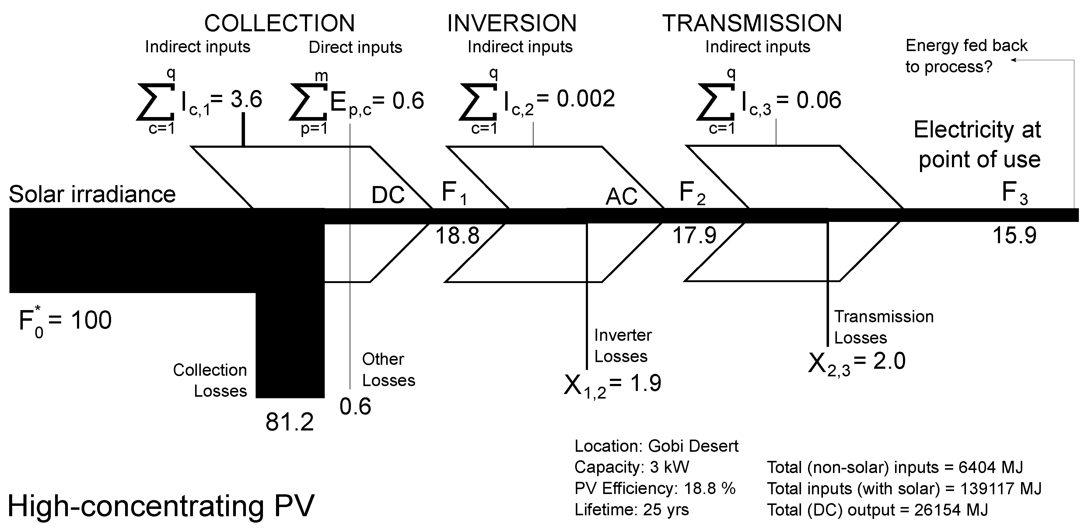
4.1. A Simple Applied Example: Solar Photovoltaic Energy Capture and Processing

A sample implementation of such a model for a photovoltaic electricity processing (collection, inversion and distribution) pathway is shown in Figure 4. There are large losses (81.2%) during the conversion of incoming solar photons to DC electrical output. The inclusion of incoming solar irradiance tends to paint PV in a bad light. To make a completely fair analysis, this should be compared with recovery (extraction) factors for crude oil which are often between 40% and 80% of oil in place in a field recovered as crude [51,52]. This initial collection loss shall not be included for computing the efficiencies nor the energy return ratios however, the CERI report suggests calculating an energy ratio which takes such losses into account for fossil fuels since unrecovered resources may be lost to future generations [10]. Subsequent conversion stages have efficiencies of 95% and 89% for inversion (conversion of DC to AC) and transmission, respectively. External energy inputs are small. Indirect (material) inputs to the collection stage are comparatively large. We may now use these values to calculate the various efficiencies and energy ratios defined earlier for each of the collection (1), inversion (2) and transmission (3) stages and for the whole system (sys) [53].

Figure 4. Electricity production from a PV panel with data from [54,55,56] modeled as an energy extraction and conversion pathway. Collection losses are neglected in this case (see text for discussion). In reality a proportion of the finished product would be fed back into the production process. Unfortunately no data are available on this.

Figure 4. Electricity production from a PV panel with data from [54,55,56] modeled as an energy extraction and conversion pathway. Collection losses are neglected in this case (see text for discussion). In reality a proportion of the finished product would be fed back into the production process. Unfortunately no data are available on this.

The resulting efficiencies and ERRs are shown in Table 4. Note that a traditional energy balance for the first process stage in this figure will result in more energy inputs than outputs. This is because the indirect consumption values I do not enter the spatial system boundary around a process (e.g., energy consumed to make steel for a solar panel frame is consumed offsite and therefore will not enter into a traditional energy balance with finite spatial boundaries). Since the production of the product does require the indirect energy consumption, it must be allocated to the processing stage of interest, despite the fact that it would not cross a traditional system boundary.

Table 4. Efficiencies and energy return ratios for the example PV production process. As discussed in the text, collection losses are omitted from the analysis.

	System Boundary
Ratios	α	β	γ	δ
${\eta }_1$	$\frac{18.8}{18.8}=1.00$	$\frac{18.8}{18.8}=1.00$	$\frac{18.8}{18.8+0.6}=0.97$	$\frac{18.8}{18.8+0.6+3.6}=0.82$
${\eta }_2$	$\frac{17.9}{18.8}=0.95$	$\frac{17.9}{18.8}=0.95$	$\frac{17.9}{18.8}=0.95$	$\frac{17.9}{18.8+0.002}=0.95$
${\eta }_3$	$\frac{15.9}{17.9}=0.89$	$\frac{15.9}{17.9}=0.89$	$\frac{15.9}{17.9}=0.89$	$\frac{15.9}{17.9+0.06}=0.89$
$GE{R}_{sys}$	-	$\frac{15.9}{1.9+2.0}=4.08$	$\frac{15.9}{1.9+2.0+0.6}=3.53$	$\frac{15.9}{1.9+2.0+0.6+3.6+0.002+0.06}=1.95$
$NE{R}_{sys}$	-	$4.08$	$3.53$	$1.95$
$GEE{R}_{sys}$	-	$\frac{15.9}{0}=\infty$	$\frac{15.9}{0.6}=26.5$	$\frac{15.9}{0.6+3.6+0.002+0.06}=3.73$
$NEE{R}_{sys}$	-	∞	$26.5$	$3.73$

Table 4. Efficiencies and energy return ratios for the example PV production process. As discussed in the text, collection losses are omitted from the analysis.

	System Boundary
Ratios	α	β	γ	δ
${\eta }_1$	$\frac{18.8}{18.8}=1.00$	$\frac{18.8}{18.8}=1.00$	$\frac{18.8}{18.8+0.6}=0.97$	$\frac{18.8}{18.8+0.6+3.6}=0.82$
${\eta }_2$	$\frac{17.9}{18.8}=0.95$	$\frac{17.9}{18.8}=0.95$	$\frac{17.9}{18.8}=0.95$	$\frac{17.9}{18.8+0.002}=0.95$
${\eta }_3$	$\frac{15.9}{17.9}=0.89$	$\frac{15.9}{17.9}=0.89$	$\frac{15.9}{17.9}=0.89$	$\frac{15.9}{17.9+0.06}=0.89$
$GE{R}_{sys}$	-	$\frac{15.9}{1.9+2.0}=4.08$	$\frac{15.9}{1.9+2.0+0.6}=3.53$	$\frac{15.9}{1.9+2.0+0.6+3.6+0.002+0.06}=1.95$
$NE{R}_{sys}$	-	$4.08$	$3.53$	$1.95$
$GEE{R}_{sys}$	-	$\frac{15.9}{0}=\infty$	$\frac{15.9}{0.6}=26.5$	$\frac{15.9}{0.6+3.6+0.002+0.06}=3.73$
$NEE{R}_{sys}$	-	∞	$26.5$	$3.73$

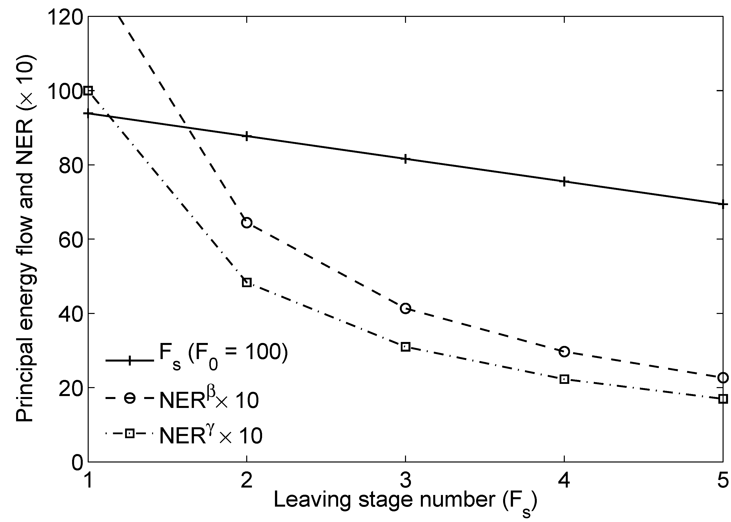
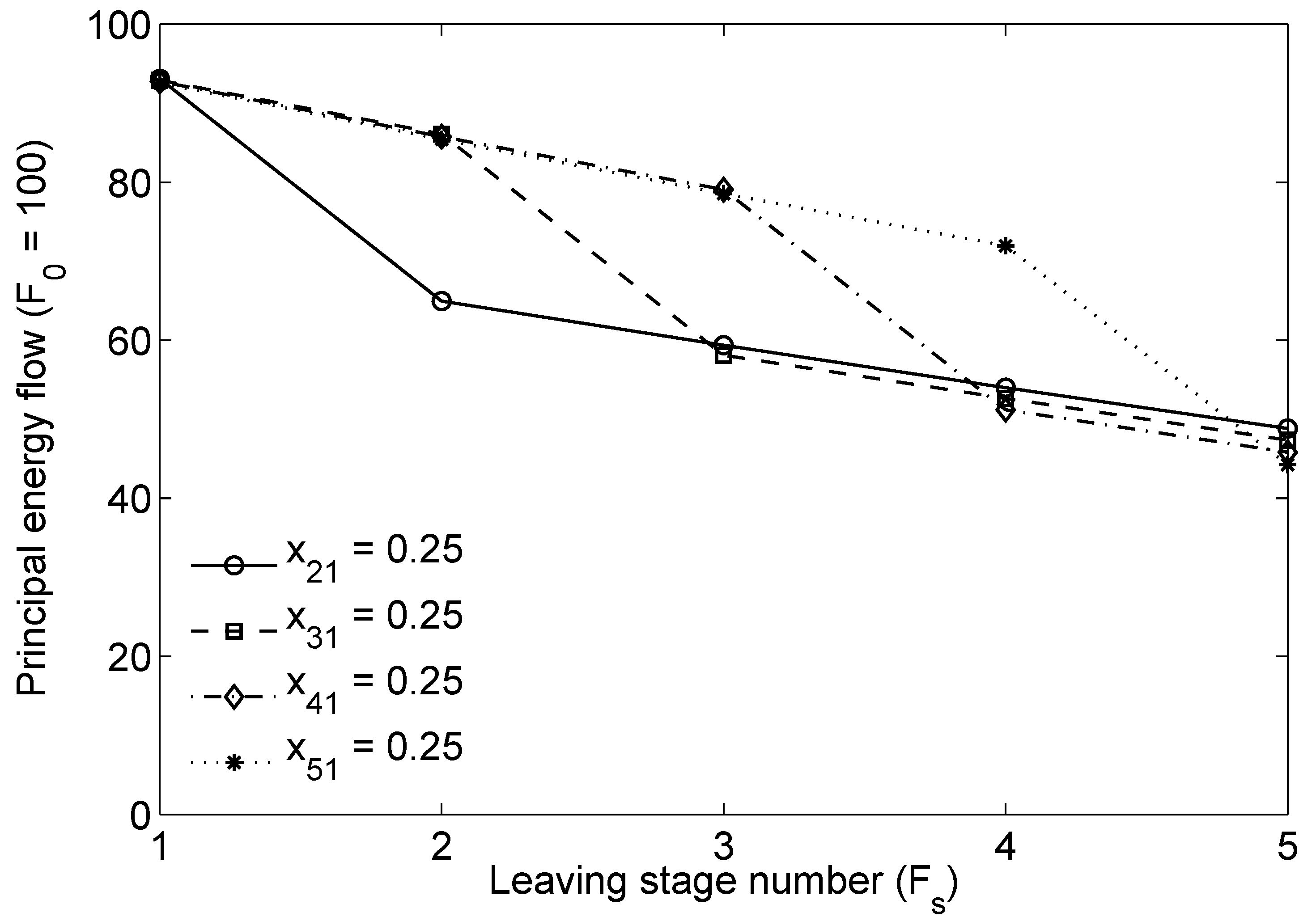
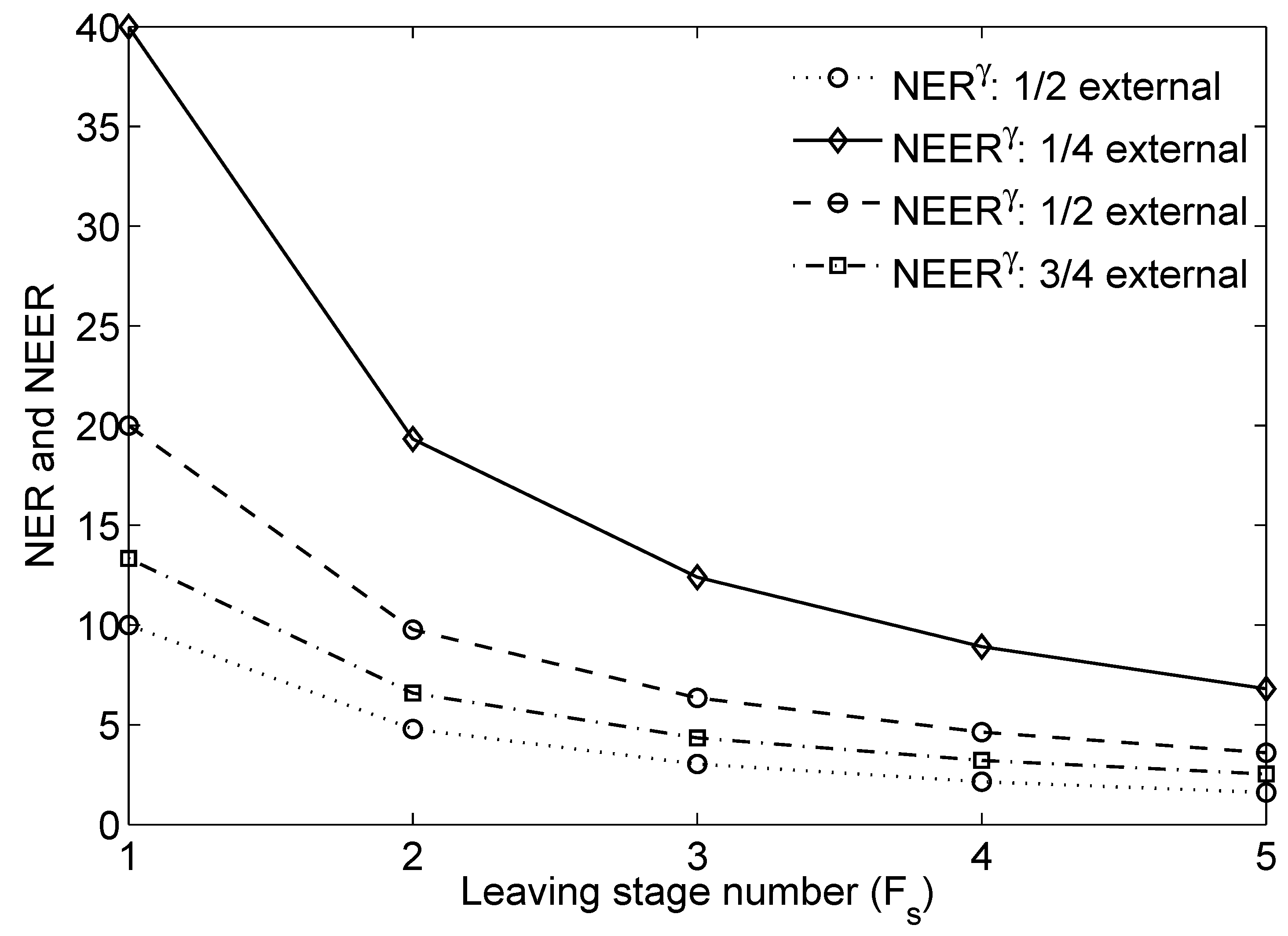
4.2. Application of Mathematical form to a Generic Energy Processing Chain

An example energy processing chain is defined below and the NER and NEER are calculated. Changes in ERRs are investigated as a function of changes in the number of processing stages, the efficiency of each stage, and the changing efficiencies at different points in the processing chain.

Figure 5 shows the reduction in principal energy flow $F_s$ as a function of processing stage s. In each stage s, all $X_{ss}$ = 0.05, while all other $X_{ft,f\ne t\ne s}$ = 0.01 (i.e., each processing stage is identical) and $X_{01}=0$. We see that by increasing the numbers of repeated identical energy processing stages, the final output $F_n^{*}$ declines linearly and the NER declines more rapidly. This behavior should be expected: as the complexity of an energy extraction and conversion pathway increases (e.g., the number of intermediate processing stages increases) the overall system NER declines because the numerator is declining while the denominator is increasing.

Figure 5. Comparison of NER${}^{\beta }$, NER${}^{\gamma }$ and $F_s$ as a function of processing stage s.

Figure 5. Comparison of NER${}^{\beta }$, NER${}^{\gamma }$ and $F_s$ as a function of processing stage s.

Figure 6 shows the effect of changing a processing stage efficiency at the beginning of a pathway and at the end of a pathway. From each stage there is a large backward flow to stage 1. As we can see, endpoint flow $F_n^{*}$ declines more if the increased energy consumption occurs at the end of the processing chain. This is because increased consumption at the end of the processing chain is amplified into a larger required volume as it moves “back up” the processing chain. Returning to our example of the oil pathway, reducing gasoline consumption by 100 units reduces total primary energy consumption by more than 100 units due to the upstream burdens of supplying primary energy to extract and refine oil into gasoline.

Figure 6. Comparison of final energy output given changes in location of large processing energy input. Note that a processing intensive technology further in the processing chain results in less final energy output.

Figure 6. Comparison of final energy output given changes in location of large processing energy input. Note that a processing intensive technology further in the processing chain results in less final energy output.

Next, Figure 7 shows the effect of keeping the overall efficiency of each processing chain constant using the broadest efficiency metric ${\eta }^{\delta }$ but substituting external energy consumption for internal. In this case, we see a divergence between NER and NEER, due to changing emphasis on internal and external sources of energy. The NEER becomes an increasingly less accurate metric of overall system consumption as a larger fraction of the energy is provided internally.

Figure 7. Comparison between EER${}^{\gamma }$ and NER${}^{\gamma }$ with changes in the makeup of consumption between internal (X) and external (E) consumption. In all cases indirect consumption is equal to 0.

Figure 7. Comparison between EER${}^{\gamma }$ and NER${}^{\gamma }$ with changes in the makeup of consumption between internal (X) and external (E) consumption. In all cases indirect consumption is equal to 0.

5. Discussion of Formulation Limitations and Next Steps

The formulations derived here aim to provide rigorous frameworks for bottom-up ERRs. This is a step forward, as the specification of these ratios is often not stated explicitly by authors when calculating values of ERRs. Future work will investigate the alignment of our model with previously published standards for EROI methods and explore additional ERRs that have been proposed in the literature.

Limitations remain in generating robust, unambiguous figures for ERRs. External ERRs are uncertain due to the fact that each external energy source has its own associated pathway, with losses and processing stages similar to those in the pathway being analyzed. Stated differently, it is somewhat simplistic to separate out a single energy extraction and conversion pathway from others, because the NER of a given energy extraction and conversion pathway is dependent on the NER of all other input energy types that are directly and indirectly consumed in it. The application of hybrid-EIO methods from the life cycle analysis literature serves to address these concerns. Alternatively, a simultaneous multi-pathway model could be specified for all major energy extraction and conversion pathways. This would increase the complexity of the model significantly.

Second, life cycle ERRs suffer similar difficulties as life cycle analysis in general [32,33]: system boundary truncation, uncertainty, co-product allocation, and others. The use of a hybrid-EIO LCA model addresses some of these concerns, but faces its own limitations [38]. For example, EIO-based models are inherently linear in scaling, they are static snapshots of a single period in time, and are limited by the granularity of the dataset underlying the model (in the Carnegie Mellon University EIO-LCA model, the economy is divided into ≈500 sectors, which limits the specificity with which indirect materials and services burdens can be modeled) [43].

Third, the current model does not account for the quality of energy resources of different types. It sums all energy types by their thermal energy equivalents, and does not adjust for the thermodynamic quality or convenience of the resource. A useful extension of the model would be to adjust all flows by their thermodynamic quality (e.g., exergy) [57] or by the economic divisia index [58,59].

Next, in reality, all of these functions are dynamic and effectively correlated across years: the expenditure of energy embodied in steel allows for expansion of production or transformation in future years. Or in another case, a lower NER today can correspond to a higher NER in the future if capital investment is used to increase the efficiency of a process. In order to address this “auto-catalytic” dynamic aspect of the system, a much more complex dynamic model would be required. This is left as future work.

Fifth, the complexity of energy extraction and conversion pathways is typically greater than the simple linear pathway assumed here. For example, in an oil extraction and conversion pathway, after the refining stage, the resulting flows are separated and consumed in a variety of end-use sectors (e.g., LPG vs. bunker fuels used in international shipping). This results in a fragmentation of the pathway. One consistent approach to deal with this difficulty would be to generate a series of pathways, each defined by a different end-product energy type that is consumed by society.

Lastly, systems analysis of the sort practiced in NEA is subject to irreducible uncertainties associated with data availability, the complexity of energy extraction and conversion pathways, and the ever-shifting nature of energy technologies. Therefore any energy return ratio calculated is only an approximation, even if a specific and unambiguous calculation framework is used.

6. Appendix: Derivation of Multi-Stage, Single-Pathway Models

This appendix outlines in detail the derivation of the functional forms presented in Table 1, Table 2, and Table 3.

In each model, two activities take place. In a processing stage some energy is consumed (or, more properly, the exergy contained in the energy is consumed, and the energy source is brought into equilibrium with the environment). At a distribution point no energy is consumed, but the flow of principal energy is divided for consumption elsewhere in the system.

6.1. Two Stage Pathways with Only Internal Consumption

The simplest pathway contains two processing stages that can only consume principal energy internally as it passes through the processing stages (see Figure 8).

Figure 8. Energy production process with one pathway and two stages of only internal consumption.

Figure 8. Energy production process with one pathway and two stages of only internal consumption.

6.1.1. Energy Balance

The energy balance across the processing stages are as follows:

$$S_1:\stackrel{IN}{\overbrace{F_0^{*}}}=\stackrel{OUT}{\overbrace{F_1+X_{01}}}$$

(6)

$$S_2:\stackrel{IN}{\overbrace{F_1^{*}}}=\stackrel{OUT}{\overbrace{F_2+X_{12}}}$$

(7)

where F terms are the principal energy flow that is being processed and X is self-energy consumed in the process (e.g., principal energy flow that is consumed within the processing stage). Flow $X_{01}$ will often not be used because the energy extracted cannot be used in the first process before it is harvested (e.g., crude oil in the ground cannot be used before it is lifted from the ground, or energy from sunlight must first be harvested before it can be used). Examples of $X_{01}$ include reservoir energy (pressure) used for lifting crude oil that is not part of the chemical energy content of the crude, or oil production processes based on in situ combustion.

The energy balance across the distribution points are simple:

$$D_1:\stackrel{IN}{\overbrace{F_1}}=\stackrel{OUT}{\overbrace{F_1^{*}}}$$

(8)

$$D_2:\stackrel{IN}{\overbrace{F_2}}=\stackrel{OUT}{\overbrace{F_2^{*}}}$$

(9)

6.1.2. Efficiencies

It is useful to define an efficiency of conversion for the processing stages. ${\eta }^{\alpha }$ is called the flow through efficiency because this simple model only considers principal energy flowing through the stages. It is defined as the ratio of useful energy outputs to total energy inputs:

$${\eta }_1^{\alpha }=\frac{F_1}{F_0^{*}}$$

(10)

$${\eta }_1^{\alpha }=\frac{F_2}{F_1^{*}}$$

(11)

Also, we can define a normalized fraction φ for the distribution point that represents how much of the principal energy stream leaves the distribution point to the next processing stage (as compared to being used for consumption elsewhere in the chain):

$${\varphi }_1=\frac{F_1^{*}}{F_1}=1$$

(12)

$${\varphi }_2=\frac{F_2^{*}}{F_2}=1$$

(13)

While these ratios are perhaps uninteresting in this simple case, they become useful in more complex cases.

6.1.3. Net Energy Ratio and Other Energy Return Ratios

We are now able to define the net energy ratio in terms of the absolute magnitudes of energy consumed

$$NE{R}_2^{\alpha }=\frac{F_2^{*}}{X_{01}+X_{12}}$$

(14)

$$GE{R}_2^{\alpha }=\frac{F_2}{X_{01}+X_{12}}$$

(15)

Note that these quantities are identical in the current case (they will diverge in more complex models below). Using our relationships derived above, NER and GER can also be defined in terms of our normalized quantities (efficiencies and distribution point fractional pass-through):

$$NE{R}_2^{\alpha }=\frac{{\varphi }_1{\varphi }_2{\eta }_1^{\alpha }{\eta }_2^{\alpha }}{1-{\varphi }_1{\eta }_1^{\alpha }{\eta }_2^{\alpha }}$$

(16)

Although not needed here, we leave in the φ terms (=1) for congruence with later model versions. The gross energy ratio is defined similarly:

$$GE{R}_2^{\alpha }=\frac{{\varphi }_1{\eta }_1^{\alpha }{\eta }_2^{\alpha }}{1-{\varphi }_1{\eta }_1^{\alpha }{\eta }_2^{\alpha }}$$

(17)

The external energy ratios are defined simply because there are no external inputs to our isolated system:

$$NEE{R}_1^{\alpha }=\frac{F_1^{*}}{0}=\infty$$

(18)

$$GEE{R}_1^{\alpha }=\frac{F_1}{0}=\infty$$

(19)

6.2. Two Stage Pathways with only Within-Pathway Consumption

The model above can be generalized to two stages that include within-pathway consumption, as shown in Figure 9. The consideration of system boundaries discussed above is relevant here to the specification of the self consumption flow X. Note that we consider the output energy that is self-consumed by the process to be an external energy flow that leaves the system and then returns. In this case we follow the CERI convention in considering consumption of energy output from the process as external to the processing stage boundary [10].

Figure 9. Energy production process with one pathway and two stages.

Figure 9. Energy production process with one pathway and two stages.

6.2.1. Energy Balance

There are now two energy balance terms, one for each processing stage P:

$$S_1:\stackrel{IN}{\overbrace{F_0^{*}+X_{11}+X_{21}}}=\stackrel{OUT}{\overbrace{F_1+X_{01}+X_{11}+X_{21}}}$$

(20)

$$S_2:\stackrel{IN}{\overbrace{F_1^{*}+X_{22}}}=\stackrel{OUT}{\overbrace{F_2+X_{12}+X_{22}}}$$

(21)

Or, simplifying these equations:

$$S_1:\stackrel{IN}{\overbrace{F_0^{*}}}=\stackrel{OUT}{\overbrace{F_1+X_{01}}}$$

(22)

$$S_2:\stackrel{IN}{\overbrace{F_1^{*}}}=\stackrel{OUT}{\overbrace{F_2+X_{12}}}$$

(23)

These equations are dependent on each other (each contains (implicitly) $F_1$) and therefore must be solved simultaneously [60].

The distribution points have the following energy balances:

$$D_1:\stackrel{IN}{\overbrace{F_1}}=\stackrel{OUT}{\overbrace{F_1^{*}+X_{11}}}$$

(24)

$$D_2:\stackrel{IN}{\overbrace{F_2}}=\stackrel{OUT}{\overbrace{F_2^{*}+X_{21}+X_{22}}}$$

(25)

6.2.2. Efficiencies

${\eta }^{\alpha }$ is defined similarly as above: ${\eta }_1^{\alpha }=\frac{F_1}{F_0}$, ${\eta }_2^{\alpha }=\frac{F_2}{F_1^{*}}$. ${\eta }^{\beta }$ is also defined similarly as above:

$${\eta }_1^{\beta }=\frac{F_1}{F_0+X_{11}+X_{21}},{\eta }_2^{\beta }=\frac{F_2}{F_1^{*}+X_{22}}$$

(26)

The distribution fractional pass-through terms are defined as above:

$${\varphi }_1=\frac{F_1^{*}}{F_1},{\varphi }_2=\frac{F_2^{*}}{F_2}$$

(27)

6.2.3. Net Energy Ratio and Other Energy Return Ratios

Using the above η and φ terms, the GER and NER can now be defined easily in both flow formulation and efficiency formulation:

$$\begin{array}{ccc}\hfill NE{R}_2^{\beta }& =& \frac{F_2^{*}}{X_{11}+X_{12}+X_{21}+X_{22}}\hfill \end{array}$$

(28)

$$\begin{array}{ccc}& =& \frac{{\varphi }_1{\varphi }_2{\eta }_1^{\alpha }{\eta }_2^{\alpha }}{{\eta }_1^{\alpha }(\frac{1}{{\eta }_1^{\beta }}-1)+{\varphi }_1{\eta }_1^{\alpha }{\eta }_2^{\alpha }(\frac{1}{{\eta }_2^{\beta }}-1)}\hfill \end{array}$$

(29)

$$\begin{array}{ccc}\hfill GE{R}_2^{\beta }& =& \frac{F_2}{X_{11}+X_{12}+X_{21}+X_{22}}\hfill \end{array}$$

(30)

$$\begin{array}{ccc}& =& \frac{{\varphi }_1{\eta }_1^{\alpha }{\eta }_2^{\alpha }}{{\eta }_1^{\alpha }(\frac{1}{{\eta }_1^{\beta }}-1)+{\varphi }_1{\eta }_1^{\alpha }{\eta }_2^{\alpha }(\frac{1}{{\eta }_2^{\beta }}-1)}\hfill \end{array}$$

(31)

While ${\eta }_1^{\alpha }$ can be factored out of the numerator and denominator of the efficiency formulation, we leave it here because it is useful in the n-stage model for writing the model in compact notation. If we revert to the simpler formulation above (only internal consumption) then ${\eta }^{\beta }={\eta }^{\alpha }$ and the NER and GER functions revert to their forms derived above.

The external energy ratios are still not useful metrics due to the lack of external energy inputs:

$$GEE{R}_2^{\beta }=\frac{F_2}{0}=\infty$$

(32)

$$NEE{R}_2^{\beta }=\frac{F_2^{*}}{0}=\infty$$

(33)

6.3. One Pathway, n Stages

The above results can be generalized to an $n-$stage process (this derivation is as above), as shown in Figure 10.

Figure 10. Energy production process with one pathway and n stages.

Figure 10. Energy production process with one pathway and n stages.

6.3.1. Energy Balance

For a given process stage s of the n total processes in the pathway:

$$S_s:\stackrel{IN}{\overbrace{F_{s-1}^{*}+\sum _{f=1}^n{X}_{fs}-X_{s-1,s}}}=\stackrel{OUT}{\overbrace{F_s+\sum _{f=1}^n{X}_{fs}}}$$

(34)

or

$$S_s:\stackrel{IN}{\overbrace{F_{s-1}^{*}}}=\stackrel{OUT}{\overbrace{F_s+X_{s-1,s}}}$$

(35)

With the exception of the last distribution point, the distribution points have energy balances such that:

$$D_s:\stackrel{IN}{\overbrace{F_s}}=\stackrel{OUT}{\overbrace{F_s^{*}+\sum _{t=1}^n{X}_{st}-X_{s,s+1}}}$$

(36)

while the last distribution point has the following energy balance:

$$D_n:\stackrel{IN}{\overbrace{F_n}}=\stackrel{OUT}{\overbrace{F_n^{*}+\sum _{t=1}^n{X}_{nt}}}$$

(37)

6.3.2. Efficiencies and Normalized Quantities

Flow efficiency for stage s:

$${\eta }_s^{\alpha }=\frac{F_s}{F_{s-1}}$$

(38)

Downstream flow efficiencies are the product of the upstream flow efficiencies. This result is to be expected due to the cumulative losses from upstream stages affecting all downstream stages as well. For example, for the last stage n:

$$\frac{F_n^{*}}{F_0}=\prod _{s=1}^n{\varphi }_s{\eta }_s^{\alpha }$$

(39)

For all stages except the first, the consumptive efficiencies are defined as:

$${\eta }_s^{\beta }=\frac{F_s}{F_{s-1}^{*}+{\displaystyle \sum _{f=1}^n}{X}_{fs}-X_{s-1,s}}$$

(40)

While the consumptive efficiency for the first stage is defined as:

$${\eta }_1^{\beta }=\frac{F_1}{F_0^{*}+{\displaystyle \sum _{f=0}^n}{X}_{f1}}$$

(41)

6.3.3. Energy Return Ratios

Defining the NER and GER using absolute magnitudes is straightforward:

$$NE{R}_n^{\beta }=\frac{F_n^{*}}{X_{01}+{\displaystyle \sum _{f=1}^n}{\displaystyle \sum _{t=1}^n}{X}_{ft}}$$

(42)

$$GE{R}_n^{\beta }=\frac{F_n}{X_{01}+{\displaystyle \sum _{f=1}^n}{\displaystyle \sum _{t=1}^n}{X}_{ft}}$$

(43)

We can generalize to n-stages using our efficiency based notation:

$$NE{R}_n^{\beta }=\frac{{\displaystyle \prod _{s=1}^n}{\varphi }_s{\eta }_s^{\alpha }}{{\displaystyle \prod _{s=1}^1}{\varphi }_{s-1}{\eta }_s^{\alpha }\left(\frac{1}{{\eta }_1^{\beta }}-1\right)+\cdots +{\displaystyle \prod _{s=1}^n}{\varphi }_{s-1}{\eta }_s^{\alpha }\left(\frac{1}{{\eta }_n^{\beta }}-1\right)}$$

(44)

In this case, note that we define a special term ${\varphi }_0$ for allowing compact notation. In this case, ${\varphi }_0$ represents the fraction of incoming raw energy that enters the first process, and is equal to 1 in all cases. That is, we assume that raw energy cannot be diverted to be used in other process stages before it is produced using the first process stage. This is despite the fact that some raw energy can be used in the production of raw energy (e.g., oil field pressure consumed in producing oilfield fluids).

This derivation shows the expected result that ERRs are a function only of the efficiencies of processes η, and the number of conversion processes, as should be expected. Intuitively, the more energy conversions applied between the primary energy resource and the final energy type, the less efficient the entire conversion pathway (assuming all else equal).

As should be expected, the NEER and GEER from above do not change and are undefined (equivalently $=\infty$).

6.4. One Pathway, n Stages, with External Energy Inputs

Given that each energy processing sector does not exist in isolation from all other sectors, allowance must be made for external energy inputs (e.g., energy inputs from other principal flows and pathways than the one currently under consideration). One example would be the use of coal-fired electricity in the production of PV solar panels.

An illustration of adding external energy inputs is shown in Figure 11.

Figure 11. Energy production process with one pathway and n stages and external energy inputs from outside the production pathway.

Figure 11. Energy production process with one pathway and n stages and external energy inputs from outside the production pathway.

6.4.1. Energy Balance

For process s of the n total processes in the single energy sector:

For a general process stage:

$$S_s:\stackrel{IN}{\overbrace{F_{s-1}^{*}+\sum _{f=1}^n{X}_{fs}-X_{s-1,s}+\sum _{p=1}^m{E}_{ps}}}=\stackrel{OUT}{\overbrace{F_s+\sum _{f=1}^n{X}_{fs}+\sum _{p=1}^m{E}_{ps}}}$$

(45)

where there are m other indirect energy inputs types E, defined with a counter index $p\in 1,\dots ,m$. Because we assume (as above) that external energy inputs are not incorporated into the main process flow, all external energy consumed E must leave as waste heat:

$$S_s:\stackrel{IN}{\overbrace{F_{s-1}^{*}}}=\overbrace{F_s-X_{s-1,s}}$$

(46)

This assumption may limit the ability to accurately model some pathways. For example, energy from purchased natural gas finds its way into the crude oil stream. In most cases, this simplification will not have a major effect of the EROI, and neglecting this possibility simplifies the formulation considerably. Future work can address this issue.

6.4.2. Efficiencies

The flow efficiency remains as above. The consumptive efficiency now becomes (all stages except stage 1):

$${\eta }_s^{\gamma }=\frac{F_s}{F_{s-1}^{*}+{\displaystyle \sum _{f=1}^n}{X}_{fs}-X_{s-1,s}+{\displaystyle \sum _{p=1}^m}{E}_{ps}}$$

(47)

and the first stage ${\eta }^{\gamma }$ can be defined as shown above from the energy balance.

6.4.3. Net Energy Ratio

The NER and GER in flow formulation change to include external energy inputs:

$$NE{R}_n^{\gamma }=\frac{F_n^{*}}{X_{01}+{\displaystyle \sum _{f=1}^n}{\displaystyle \sum _{t=1}^n}{X}_{ft}+{\displaystyle \sum _{p=1}^m}{\displaystyle \sum _{s=1}^n}{E}_{ps}}$$

(48)

$$GE{R}_n^{\gamma }=\frac{F_n}{X_{01}+{\displaystyle \sum _{f=1}^n}{\displaystyle \sum _{t=1}^n}{X}_{ft}+{\displaystyle \sum _{p=1}^m}{\displaystyle \sum _{s=1}^n}{E}_{ps}}$$

(49)

Or, in efficiency notation notation by simply replacing ${\eta }^{\beta }$ with ${\eta }^{\gamma }$:

$$NE{R}_n^{\beta }=\frac{{\displaystyle \prod _{s=1}^n}{\varphi }_s{\eta }_s^{\alpha }}{{\displaystyle \prod _{s=1}^1}{\varphi }_{s-1}{\eta }_s^{\alpha }\left(\frac{1}{{\eta }_1^{\gamma }}-1\right)+\cdots +{\displaystyle \prod _{s=1}^n}{\varphi }_{s-1}{\eta }_s^{\alpha }\left(\frac{1}{{\eta }_n^{\gamma }}-1\right)}$$

(50)

The GEER and NEER can now be defined in both flow and efficiency notation because external energy inputs now exist:

$$NEE{R}_n^{\gamma }=\frac{F_n^{*}}{{\displaystyle \sum _{p=1}^m}{\displaystyle \sum _{s=1}^n}{E}_{ps}}$$

(51)

$$GEE{R}_n^{\gamma }=\frac{F_n}{{\displaystyle \sum _{p=1}^m}{\displaystyle \sum _{s=1}^n}{E}_{ps}}$$

(52)

Or in efficiency notation:

$$NEE{R}_n^{\beta }=\frac{{\displaystyle \prod _{s=1}^n}{\varphi }_s{\eta }_s^{\alpha }}{{\displaystyle \prod _{s=1}^1}{\varphi }_{s-1}{\eta }_s^{\alpha }\left(\frac{1}{{\eta }_1^{\gamma }}-\frac{1}{{\eta }_1^{\beta }}\right)+\cdots +{\displaystyle \prod _{s=1}^n}{\varphi }_{s-1}{\eta }_s^{\alpha }\left(\frac{1}{{\eta }_n^{\gamma }}-\frac{1}{{\eta }_n^{\beta }}\right)}$$

(53)

6.4.4. Pathways with Indirect Consumption of Energy

Figure 12 shows for the first time a differentiation between final energy use to the rest of society and final energy use consumed indirectly in the energy sector itself (called indirect consumption). This indirect consumption arises because energy is required to supply the external energy inputs and materials consumed in the processing stages. In general, indirect consumption can arise from two sources:

• Indirect consumption of all energy types due to external energy consumption;
• Indirect consumption of all energy types due to materials consumption in the energy system.

Additionally, this indirect consumption has two effects on energy ratios:

• Indirect consumption of all energy types must be added to the denominator of the NER, GER and EER equivalents;
• Indirect consumption of the principal energy flow must be subtracted from that energy available due to the production process (e.g., must be removed from the numerator of the ratios).

Indirect consumption is difficult to model. Economic input-output (EIO) based life cycle assessment (EIO-LCA) has been used to track these direct and indirect consumptive factors [38]. Including these shifts our model system boundaries from being a purely “bottom-up” process model to a “hybrid” process-EIO model, or a hybrid EROI calculation. Indirect consumption is included in our model with symbol I. It can occur due to production of materials and energy, and therefore there is a different number of indirect consumption sources (q total) than external energy inputs.

After the total amount of energy consumed is increased through indirect consumption, the amount of this indirect energy that comes from our pathway of interest must be removed from the numerator. That is, indirect consumption not only increases the total amount of energy consumed but also reduces the useful output energy available to the rest of society. For example, in an oil pathway model, we must remove the amount of gasoline and diesel from $F_n^{*}$ that were consumed (indirectly) in the production of coal and natural gas that were consumed as external energy in our pathway, as well as any gasoline and diesel consumed to make the steel used in our process stages. Again, a hybrid process-EIO would be a methodology to use here.

Figure 12. Energy production process with one pathway and n stages, including external (E) and indirect (I) energy inputs.

Figure 12. Energy production process with one pathway and n stages, including external (E) and indirect (I) energy inputs.

We consider the term $r_i$ the fraction of indirect energy that is derived from our pathway of interest. This fractional consumption value is dependent on the action of the economy. In our simplified case, the total primary energy shares in the economy are used. For example, if 40% of total primary energy supply to society comes from oil ($r_i=0.4$), 40% of the energy burden of cement or other material input embodied energy can be removed from the useful oil output. More rigorously, economic input output analysis could be used to generate a sector-specific breakdown between energy inputs to a type of material input [38]. This rigorous approach is an application of a “hybrid” process-model EIO-LCA approach to material flow accounting. As an example of the deviation from economy-wide averages, while oil represents approximately 40% of total primary energy supply, it only represents some 15% of the energy inputs per dollar of output from the cement industry [38]. We leave the mathematical treatment of that problem for future work.

6.4.5. Energy Balance

Because indirect energy is consumed offsite and (generally) at a different time than the operation of the process, for process s of the n total processes in the single energy sector the energy balance does not change:

$$S_s:\stackrel{IN}{\overbrace{F_{s-1}^{*}+\sum _{f=1}^n{X}_{fs}-X_{s-1,s}+\sum _{p=1}^m{E}_{ps}}}=\stackrel{OUT}{\overbrace{F_s+\sum _{f=1}^n{X}_{fs}+\sum _{p=1}^m{E}_{ps}}}$$

(54)

6.4.6. Efficiencies

Our efficiencies are extended to a life cycle efficiency from above to include indirect energy consumption due to external energy inputs and materials energy inputs (all stages except first stage):

$${\eta }_s^{\delta }=\frac{F_s}{F_{s-1}+{\displaystyle \sum _{f=1}^n}{X}_{fs}-X_{s-1,s}+{\displaystyle \sum _{p=1}^m}{E}_{ps}+{\displaystyle \sum _{c=1}^q}{I}_{cs}}$$

(55)

The efficiency of the first stage is defined analogously to the above derivation.

6.4.7. Net Energy Ratio and Gross Energy Ratio

Similarly to above, the NER must change to account for the fact that the useful energy that the non-energy sector portions of the economy can access are less than the output from the final stage $F_n$, due to indirect consumption of the final energy product during materials manufacture. For example, if production pathway being analyzed produces oil, any oil consumed in making cement and steel for oil field facilities should be subtracted from $F_n$.

$$NE{R}_n^{\delta }=\frac{F_n^{*}-r_i{\displaystyle \sum _{c=1}^q}{\displaystyle \sum _{s=1}^n}{I}_{cs}}{X_{01}+{\displaystyle \sum _{f=1}^n}{\displaystyle \sum _{t=1}^n}{X}_{ft}+{\displaystyle \sum _{p=1}^m}{\displaystyle \sum _{s=1}^n}{E}_{ps}+{\displaystyle \sum _{c=1}^q}{\displaystyle \sum _{s=1}^n}{I}_{cs}}$$

(56)

$$GE{R}_n^{\delta }=\frac{F_n}{X_{01}+{\displaystyle \sum _{f=1}^n}{\displaystyle \sum _{t=1}^n}{X}_{ft}+{\displaystyle \sum _{p=1}^m}{\displaystyle \sum _{s=1}^n}{E}_{ps}+{\displaystyle \sum _{c=1}^q}{\displaystyle \sum _{s=1}^n}{I}_{cs}}$$

(57)

Or, converting NER to an efficiency-based metric:

$$NE{R}_n^{\beta }=\frac{{\displaystyle \prod _{s=1}^n}{\varphi }_s{\eta }_s^{\alpha }-r_i{\displaystyle \sum _{j=1}^n}\left[{\displaystyle \prod _{s=1}^j}{\varphi }_{s-1}{\eta }_s^{\alpha }\left(\frac{1}{{\eta }_j^{\delta }}-\frac{1}{{\eta }_j^{\gamma }}\right)\right]}{{\displaystyle \prod _{s=1}^1}{\varphi }_{s-1}{\eta }_s^{\alpha }\left(\frac{1}{{\eta }_1^{\delta }}-1\right)+\cdots +{\displaystyle \prod _{s=1}^n}{\varphi }_{s-1}{\eta }_s^{\alpha }\left(\frac{1}{{\eta }_n^{\delta }}-1\right)}$$

(58)

6.4.8. External Energy Ratio

The net external energy ratio can be easily defined:

$$NEE{R}_n^{\beta }=\frac{{\displaystyle \prod _{s=1}^n}{\varphi }_s{\eta }_s^{\alpha }-r_i{\displaystyle \sum _{j=1}^n}\left[{\displaystyle \prod _{s=1}^j}{\varphi }_{s-1}{\eta }_s^{\alpha }\left(\frac{1}{{\eta }_j^{\delta }}-\frac{1}{{\eta }_j^{\gamma }}\right)\right]}{{\displaystyle \prod _{s=1}^1}{\varphi }_{s-1}{\eta }_s^{\alpha }\left(\frac{1}{{\eta }_1^{\delta }}-\frac{1}{{\eta }_1^{\beta }}\right)+\cdots +{\displaystyle \prod _{s=1}^n}{\varphi }_{s-1}{\eta }_s^{\alpha }\left(\frac{1}{{\eta }_n^{\delta }}-\frac{1}{{\eta }_n^{\beta }}\right)}$$

(59)

References and Notes

1. Herendeen, R.A. Net energy analysis: Concepts and methods. In Encyclopedia of Energy; Ayres, R.U., Costanza, R., Goldemberg, J., Ilic, M.D., Jochem, E., Kaufmann, R., Lovins, A.B., Munasinghe, M., Pachauri, R.K., Pardo, C.S., Peterson, P., Schipper, L., Slade, M., Smil, V., Worrell, E., Cleveland, C.J., Eds.; Elsevier: Amsterdam, The Netherlands, 2004. [Google Scholar]
2. Huettner, D.A. Net energy analysis: An economic assessment. Science 1976, 192, 101–104. [Google Scholar] [CrossRef] [PubMed]
3. Cleveland, C.J. Energy quality and energy surplus in the extraction of fossil fuels in the US. Ecol. Econ. 1992, 1992, 139–162. [Google Scholar] [CrossRef]
4. Cleveland, C.J. Net energy from the extraction of oil and gas in the United States. Energy 2005, 30, 769–782. [Google Scholar] [CrossRef]
5. Pacca, S.; Sivaraman, D.; Keoleian, G.A. Parameters affecting the life cycle performance of PV technologies and systems. Energy Policy 2007, 35, 3316–3326. [Google Scholar] [CrossRef]
6. Knapp, K.; Jester, T. Empirical investigation of the energy payback time for photovoltaic modules. Sol. Energy 2001, 71, 165–172. [Google Scholar] [CrossRef]
7. EROI is sometimes called the energy return on energy invested, or EROEI.
8. Hall, C.A.S.; Balogh, S.; Murphy, J. What is the minimum EROI that a sustainable society must have? Energies 2009, 2, 25–47. [Google Scholar] [CrossRef]
9. Odum, H.T. Environment, Power, and Society; Wiley-Interscience: New York, NY, USA, 1971. [Google Scholar]
10. CERI. Net Energy Analysis: An Energy Balance Study of Fossil Fuel Resources; Colorado Energy Research Institute: Golden, CO, USA, 1976. [Google Scholar]
11. Spreng, D.T. Net Energy Analysis and the Energy Requirements of Energy Systems; Praeger Publishers: New York, NY, USA, 1988. [Google Scholar]
12. Hannon, B. Energy discounting. In Energetics and Systems; Mitsch, W.J., Ragade, R., Bosserman, R.W., Dillion, J.A.J., Eds.; Ann Arbor Science: Ann Arbor, MI, USA, 1982. [Google Scholar]
13. Spitzley, D.V.; Keoleian, G. Life Cycle Environmental and Economic Assessment of Willow Biomass Electricity: A Comparison with Other Renewable and Non-Renewable Sources; Technical Report CSS04-05R; University of Michigan: Ann Arbor, MI, USA, 2004. [Google Scholar]
14. Mulder, K.; Hagens, N.J. Energy return on investment: Toward a consistent framework. AMBIO: J. Hum. Environ. 2008, 37, 74–79. [Google Scholar] [CrossRef]
15. Murphy, D.J.; Hall, C.A.S.; Cleveland, C.J. Order from chaos: A preliminary protocol for determining EROI for fuels. In Presented at the Association for Study of Peak Oil-USA Conference, Boston, MA, USA, 25–27 October 2006.
16. Brandt, A.R. Converting oil shale to liquid fuels: Energy inputs and greenhouse gas emissions of the Shell in situ conversion process. Environ. Sci. Technol. 2008, 42, 7489–7495. [Google Scholar] [CrossRef] [PubMed]
17. Brandt, A.R. Converting oil shale to liquid fuels with the Alberta Taciuk Processor: Energy inputs and greenhouse gas emissions. Energy & Fuels 2009, 23, 6253–6258. [Google Scholar]
18. Norgaard, R.B. Output, Input and Productivity Change in U.S. Petroleum Development: 1939–1968. Ph.D. Thesis, University of Chicago, Chicago, IL, USA, 1971. [Google Scholar]
19. Norgaard, R.B. Resource scarcity and new technology in U.S. petroleum development. Nat. Resour. J. 1975, 15, 265–282. [Google Scholar]
20. Norgaard, R.B.; Leu, G.J. Petroleum accessibility and drilling technology-an analysis of United-States development costs from 1959 to 1978. Land Econ. 1986, 62, 14–25. [Google Scholar] [CrossRef]
21. Livernois, J.R. Empirical-evidence on the characteristics of extractive technologies-the case of oil. J. Environ. Econ. Manag. 1987, 14, 72–86. [Google Scholar] [CrossRef]
22. Livernois, J.R.; Uhler, R.S. Extraction costs and the economics of nonrenewable resources. J. Political Econ. 1987, 95, 195–203. [Google Scholar] [CrossRef]
23. Ayres, R.; Warr, B. Accounting for growth: The role of physical work. Struct. Change Econ. Dyn. 2005, 16, 181–209. [Google Scholar] [CrossRef]
24. Ayres, R. Exergy, power and work in the US economy, 1900–1998. Energy 2003, 28, 219–273. [Google Scholar] [CrossRef]
25. Ayres, R.U. Energy efficiency, sustainability, and economic growth. Energy 2007, 32, 634–638. [Google Scholar] [CrossRef]
26. Sorrell, S. Energy, Growth, and Sustainability: Five Propositions; SPRU-Science and Technology Policy Research: Colorado, CO, USA, 2010. [Google Scholar]
27. King, C.; Zarnikau, J.; Henshaw, P. Defining a Standard Measure for Whole System EROI Combining Economic “Top-Down” and LCA “Bottom-Up” Accounting. In Proceedings of the ASME 2010 4th International Conference on Energy Sustainability (ES2010), Phoenix, AZ, USA, 17–22 May 2010.
28. Henshaw, P.; King, C.; Zarnikau, J. System energy assessment (SEA), defining a standard measure of EROI for energy businesses as whole systems. Sustainability 2011, in press. [Google Scholar] [CrossRef]
29. Boulding, K. The unimportance of energy. In Energetics and Systems; Mitsch, W.J., Ragade, R., Bosserman, R.W., Dillion, J.A.J., Eds.; Ann Arbor Science: Ann Arbor, MI, USA, 1982. [Google Scholar]
30. Boulding [29] cites 7 basic “factors” or elements that are of fundamental value to an economy (or an organism): space, time, matter, energy, information, “know-how”, and “know-what”. These factors are traded off by organisms and economies, such that a company might deploy capital (at matter and energy cost) to save human labor (time). Note that fundamental theories of value can be constructed around a number of of these factors (e.g., labor theory of value).
31. Leach, G. Net energy analysis-is it any use? Energy Policy 1975, 1975, 332–344. [Google Scholar] [CrossRef]
32. Reap, J.; Roman, F.; Duncan, S.; Bras, B. A survey of unresolved problems in life cycle assessment—Part 1: Goal and scope and inventory analysis. Int. J. Life Cycle Assess. 2008, 13, 290–300. [Google Scholar] [CrossRef]
33. Reap, J.; Roman, F.; Duncan, S.; Bras, B. A survey of unresolved problems in life cycle assessment—Part 2: Impact assessment and interpretation. Int. J. Life Cycle Assess. 2008, 13, 374–388. [Google Scholar] [CrossRef]
34. The issue of worker food consumption raises important systems boundary questions. Does one count the energy content of the workers’ food (i.e., food calories), the embodied fossil energy in the food (e.g., fertilizer energy inputs), or neither input because the worker would have eaten anyway without the energy project?
35. Bullard, C.W.; Penner, P.S.; Pilati, D.A. Net energy analysis: Handbook for combining process and input-output analysis. Resour. Energy 1978, 1, 267–313. [Google Scholar] [CrossRef]
36. An excellent analysis of the effect of system boundaries on internal vs. external accounting is given by CERI [10] (p. III-25).
37. Hendrickson, C.T.; Horvath, A.; Joshi, S.; Klausner, M.; Lave, L.B.; McMichael, F.C. Comparing two life cycle assessment approaches: A process model-vs. economic input-output-based assessment. Proceedings of the 1997 IEEE International Symposium on Electronics and the Environment 1997, 412, 176–181. [Google Scholar]
38. Hendrickson, C.T.; Lave, L.B.; Scott, M.H. Environmental Life Cycle Assessment of Goods and Services: An Input-Output Approach; Resources for the Future: Washington, DC, USA, 2006. [Google Scholar]
39. Herendeen, R.A. Input-output techniques and energy cost of commodities. Energy Policy 1978, 6, 162–165. [Google Scholar] [CrossRef]
40. It is noted here that energy is never truly “consumed” due to the first law of thermodynamics. This terminology is used throughout to refer to the degradation of useful energy to waste heat, or the destruction of exergy during an energy conversion process.
41. Note that we assume that no external energy inputs Ep end up contained within the principal energy flow Fs. This is a simplification made for ease of exposition and solution of the resulting mathematics. Also, we note that flow Xs,s also cannot be incorporated into the output energy stream. In some real-world cases, this assumption is violated, as when an oil refinery incorporates energy from natural-gas-derived hydrogen into the finished product stream.
42. Using the EIO LCA tool, very little biomass energy is consumed indirectly in natural gas production. In rounding to two significant figures, no biomass energy is consumed.
43. CMU-GDI. Economic Input-Output Life Cycle Assessment (EIO-LCA). US 2002 Industry Benchmark model. 2008. Available online: http://www.eiolca.net/ (accessed on 17 Auguest 2011).
44. If we were building a simultaneous multi-pathway model, the specific types of secondary energy resources consumed would have to be accounted in the model through other pathways. Also, thermal energy could be weighted by a physical or economic quality-weighting factor (see discussion below).
45. Wang, M.Q. Estimation of Energy Efficiencies of U.S. Petroleum Refineries (Plus Associated Spreadsheet); Center for Transportation Research, Argonne National Laboratory: Argonne, IL, USA, 2008.
46. Denholm, P.; Kulcinski, G.L. Life cycle energy requirements and greenhouse gas emissions from large scale energy storage systems. Energy Convers. Manag. 2004, 45, 2153–2172. [Google Scholar] [CrossRef]
47. ηα is derived from an energy balance on a pathway with no external consumption, as illustrated in the appendix.
48. This quantity has been called by a number of names, including Process Net Energy Ratio (PNER) [10], energy yield ratio (EYR) and net energy ratio (NER). The same CERI report also defines a related metric called the Resource Net Yield Ratio that includes in the denominator energy lost or rendered unrecoverable through the extraction process. Metrics also differ by whether they consider the gross or net output from a process.
49. In other studies, this quantity is variously called the incremental energy ratio, or IER [1], or the external net energy ratio (ENER) [10].
50. Note that methods for calculating EROI have varied significantly to date, but this metric seems the most congruent with the general goals of EROI analysis.
51. Tzimas, E.; Georgakaki, A.; Cortes, C.; Peteves, S. Enhanced Oil Recovery using Carbon Dioxide in the European Energy System; Report EUR 21895 EN; European Commission Joint Research Centre: Brussels, Belgium, December 2005. [Google Scholar]
52. Green, D.; Willhite, G. Enhanced Oil Recovery; Society of Petroleum Engineers: Richardson, TX, UAS, 1998. [Google Scholar]
53. Since there are no measured Xj,k flows between stages within the pathway under study, ηα = ηβ. Likewise, the NER, GER and the NEER and GEER are equal, since X3,j flows are unknown.
54. Ray, S. Electrical Power Systems: Concepts, Theory and Practice; Printice-Hall of India: New Delhi, India, 2007. [Google Scholar]
55. Nishimura, A.; Hayashi, Y.; Tanaka, K.; Hirota, M.; Kato, S.; Ito, M.; Araki, K.; Hu, E. Life cycle assessment and evaluation of energy payback time on high-concentration photovoltaic power generation system. Appl. Energy 2010, 87, 2797–2807. [Google Scholar] [CrossRef]
56. King, D.; Gonzalez, S.; Galbraith, G.; Boyson, W. Performance Model for Grid-Connected Photovoltaic Inverters; Sandia Report, SAND2007-5036; Sandia National Laboratories: Livermore, CA, USA, 2007. [Google Scholar]
57. Hermann, W. Quantifying global exergy resources. Energy 2006, 31, 1349–1366. [Google Scholar] [CrossRef]
58. Cleveland, C.J.; Kaufman, R.K.; Stern, D.I. Aggregation and the role of energy in the economy. Ecol. Econ. 2000, 32, 301–317. [Google Scholar] [CrossRef]
59. Cleveland, C.J.; Kaufmann, R.K.; Stern, D.L. Aggregation of energy. In Encyclopedia of Energy; Ayres, R.U., Costanza, R., Goldemberg, J., Ilic, M.D., Jochem, E., Kaufmann, R., Lovins, A.B., Munasinghe, M., Pachauri, R.K., Pardo, C.S., Peterson, P., Schipper, L., Slade, M., Smil, V., Worrell, E., Cleveland, C.J., Eds.; Elsevier: Amsterdam, The Netherlands, 2004; Volume 1. [Google Scholar]
60. This is a common feature of mathematical models with “recycle” loops (e.g., chemical engineering systems with recycle of unreacted product).