Forecasting Electricity Demand in Thailand with an Artificial Neural Network Approach

Abstract

Demand planning for electricity consumption is a key success factor for the development of any countries. However, this can only be achieved if the demand is forecasted accurately. In this research, different forecasting methods—autoregressive integrated moving average (ARIMA), artificial neural network (ANN) and multiple linear regression (MLR)—were utilized to formulate prediction models of the electricity demand in Thailand. The objective was to compare the performance of these three approaches and the empirical data used in this study was the historical data regarding the electricity demand (population, gross domestic product: GDP, stock index, revenue from exporting industrial products and electricity consumption) in Thailand from 1986 to 2010. The results showed that the ANN model reduced the mean absolute percentage error (MAPE) to 0.996%, while those of ARIMA and MLR were 2.80981 and 3.2604527%, respectively. Based on these error measures, the results indicated that the ANN approach outperformed the ARIMA and MLR methods in this scenario. However, the paired test indicated that there was no significant difference among these methods at α = 0.05. According to the principle of parsimony, the ARIMA and MLR models might be preferable to the ANN one because of their simple structure and competitive performance

1. Introduction

Electric energy is a significant driving force for economic development, while the accuracy of demand forecasts is an important factor leading to the success of efficiency planning. For this reason, energy analysts need a guideline to better choose the most appropriate forecasting techniques in order to provide accurate forecasts of electricity consumption trends. The outcome of the study might be used by the appropriate national agency in Thailand (e.g., Energy Policy and Planning Office (EPPO), Ministry of Energy) as a means to develop energy policies as well as measures on energy conservation and alternative energy. However, there are many techniques that contribute to the prediction of future electricity demand. In this study, different forecasting techniques were utilized to forecast the electricity consumption in Thailand and a comparison of these techniques was conducted to choose the best approach in this situation.

The determination of an appropriate forecasting model was based on historical data, while the error criteria such as mean squared error (MSE) and mean absolute percentage error (MAPE) were utilized as measures to justify the appropriate model. In addition to minimizing the errors, one of the most important conditions was that the residual from the forecasting model had to satisfy all the assumptions or pass the model adequacy checking (normally and independently distributed: NID). According to the literature, most forecasting models were determined from three popular methods, i.e., autoregressive integrated moving average (ARIMA), artificial neural network (ANN) and multiple linear regression (MLR) model. For time series analysis, the autoregressive integrated moving average (ARIMA) model is a stochastic difference equation that is frequently utilized to model stochastic disturbances [1]. Some specific forms of the ARIMA model were utilized to represent autocorrelated disturbances, e.g., autoregressive order one, ARIMA (1,0,0) or AR (1) for stationary disturbances, while an integrated moving average, ARIMA (0,1,1) or IMA (1,1) are used to represent non-stationary disturbances, as recommended by Montgomery, Keats, Runger and Messina [2] and Box and Luceno [3].

Ediger and Akar [4] utilized both the ARIMA and seasonal ARIMA (SARIMA) models to estimate the future primary energy demand of Turkey from 2005 to 2020. The ARIMA method was also deployed by Abdel-Aal and Al-Garni [5] to forecast monthly domestic electric energy consumption in the eastern province of Saudi Arabia and the optimum model in this case was the first ordered ARIMA with a multiplicative combination of seasonal and non-seasonal autoregressive parts. Zhou, Ang and Poh [6] improved the accuracy of electricity demand predictions by combining the traditional grey model GM (1,1) with the trigonometric residual modification technique. Additionally, Cho, Hwang and Chen [7] compared the results of the univariate ARIMA and the traditional regression models to forecast the short-term load by considering weather-load relationships.

Another forecasting approach was the utilization of the ANN method to derive a prediction model. The development of ANN models was based on studying the relationship between input variables and output variables. For application in forecasting, Hsu and Chen [8] assessed the performance of ANN approach (based on three inputs, i.e., GDP, population and temperature) to forecast the regional peak load in Taiwan. The historical data was the annual power load in each region from 1981 to 2000 and the performance of ANN method was compared with the regression method. The study showed that the error of ANN model was significantly lower than that of the regression model. Moreover, Catalao, Mariano, Mendes and Ferreira [9] successfully applied the ANN for forecasting next-week prices in the electricity market of Spain and State of California short-term electricity prices. The hourly price data of 42 days prior to the week whose prices were forecasted was used as the historical data. The error criterion (MAPE) of the ANN model was compared with the one from ARIMA model and the results indicated that the ANN outperformed the ARIMA model. Similarly, Bakirtzis, Petridis, Klartzis and Alexladis [10] developed an artificial neural network to forecast daily loads with a lead time of one to seven days. The seasonality effect from high energy usage on holidays was included in the model by utilizing the seasonal training (training the ANN with the historical holiday data).

The multiple linear regression method is still an interesting forecasting option because of its simplicity. Mohamed and Bodger [11] used a multiple linear regression model to forecast the electricity consumption of New Zealand where the independent variables were gross domestic product (GDP), electricity price and population. The genetic algorithm (GA) was integrated with an ANN in the study of Azadeh, Ghaderi, Tavedian and Saberi [12] to forecast the monthly electricity demand in Iran. The estimated errors (MAPE) were used as the measure of errors, while the results showed that the MAPE of the proposed method was less than those of regression and time series models. Moreover, Azadeh, Ghaderi and Sohrabkhani [13] also assessed the performance of an ANN model to forecast monthly electricity consumption by utilizing analysis of variance (ANOVA). Four treatments of the experiment were: actual data, time series, ANN and simulation-based ANN. According to the empirical study, ANN was superior to the time series and simulation-based ANN.

Hong [14] suggested the utilization of a support vector model (SVM) as an alternative to an ANN for forecasting electric consumption. According to the empirical study, the performance of SVM was superior to other methods, regression and ANN models. Ekonomou [15] compared the ability to predict the Greek-long term energy consumption of these three methods: ANN, regression and SVM. The results indicated that both ANN and SVM were able to forecast the consumption with great accuracy. Pappas, Ekonomou, Karamousantas, Chatzarakis, Katsikas and Liatsis [16] introduced the utilization of traditional methodology, i.e., an ARIMA model, to predict the electricity demand. Different ARIMA models were selected and the criteria (Akaike Information Criterion: AIC and Bayesian Information Criterion: BIC) were utilized to justify the most appropriate one.

Since there are no empirical or exact rules to derive the best forecasting model, the most appropriate one was selected by choosing the model with the lowest error. Mostly, the error margins of the candidate forecasting methods were slightly different. Moreover, a handful of works have contributed to compare whether there was a significant difference between the errors from each method. In this research, the performance of ANN approach and the traditional methods, i.e., ARIMA and MLR, was assessed and compared using a set of data regarding the total electricity consumption in Thailand from 1986 to 2010. For MLR, some critical factors such as the amount of exports and stock index which significantly affected the consumption were included in the forecasting model. The error (MAPE) from each method was calculated and used to rank the top performer, followed by the runner-ups. Afterwards, the Wilcoxson sign rank test and paired t-test were utilized to compare the errors from each pair of methods.

2. Historical Data

Electricity consumption (GWh) is influenced by many factors: population, gross domestic product (GDP), stock index (SET index) and total revenue from exporting industrial products (export). The historical data set regarding these factors was collected annually from 1986 to 2010 and is shown in Table 1. It was utilized as a basis to determine a forecasting model for future electricity demand.

Table 1. Energy Data of Thailand from 1986 to 2010.

Year	Population	GDP	SET Index	Export (million baht)	Electricity Consumption (GWh)
1986	52511000	1257177	207.2	364017.25	10162.7
1987	53427000	1376847	284.94	455991.43	11319.4
1988	54326000	1559804	386.73	462426.83	11942.38
1989	55214000	1749952	879.19	562426.76	14328.1
1990	55839000	1945372	612.86	683946.13	16717.23
1991	56574000	2111862	711.36	725448.79	19406.02
1992	57294000	2282572	893.42	824643.29	21641.01
1993	58010000	2470908	1682.85	940862.59	24321.28
1994	58713000	2692973	1360.09	1137601.65	27758.43
1995	59401000	2941736	1280.81	1153489	31870.37
1996	60003000	3115338	831.57	1153894.61	34607.29
1997	60602000	3072615	372.69	1492331.29	36981.24
1998	61201000	2749684	355.81	1854500.09	35154.99
1999	61806000	2871980	481.92	1871544.78	36275.13
2000	62236000	3008401	269.19	2378191.26	39546.26
2001	62836000	3073601	303.85	2454987.54	41658.51
2002	63419000	3237042	356.48	2506442.96	44805.66
2003	63982000	3468166	772.15	2857191.85	48293.79
2004	64531000	3688189	668.1	3361360.69	50810.54
2005	65099000	3858019	713.73	3897247.1	53894.12
2006	65574000	4054504	679.84	4305406.71	56994.75
2007	66041000	4259026	858.1	4691207.01	59436.12
2008	66482000	4364833	449.96	5149902.76	60266.29
2009	66903000	4263139	734.54	4619810.05	59401.92
2010	67209942.8	4595809	1032.76	5476766.65	60315.04

Source: Bank of Thailand, Department of Export Promotion, Energy Policy and Planning Office (EPPO) and Stock Exchange of Thailand.

Table 1. Energy Data of Thailand from 1986 to 2010.

Year	Population	GDP	SET Index	Export (million baht)	Electricity Consumption (GWh)
1986	52511000	1257177	207.2	364017.25	10162.7
1987	53427000	1376847	284.94	455991.43	11319.4
1988	54326000	1559804	386.73	462426.83	11942.38
1989	55214000	1749952	879.19	562426.76	14328.1
1990	55839000	1945372	612.86	683946.13	16717.23
1991	56574000	2111862	711.36	725448.79	19406.02
1992	57294000	2282572	893.42	824643.29	21641.01
1993	58010000	2470908	1682.85	940862.59	24321.28
1994	58713000	2692973	1360.09	1137601.65	27758.43
1995	59401000	2941736	1280.81	1153489	31870.37
1996	60003000	3115338	831.57	1153894.61	34607.29
1997	60602000	3072615	372.69	1492331.29	36981.24
1998	61201000	2749684	355.81	1854500.09	35154.99
1999	61806000	2871980	481.92	1871544.78	36275.13
2000	62236000	3008401	269.19	2378191.26	39546.26
2001	62836000	3073601	303.85	2454987.54	41658.51
2002	63419000	3237042	356.48	2506442.96	44805.66
2003	63982000	3468166	772.15	2857191.85	48293.79
2004	64531000	3688189	668.1	3361360.69	50810.54
2005	65099000	3858019	713.73	3897247.1	53894.12
2006	65574000	4054504	679.84	4305406.71	56994.75
2007	66041000	4259026	858.1	4691207.01	59436.12
2008	66482000	4364833	449.96	5149902.76	60266.29
2009	66903000	4263139	734.54	4619810.05	59401.92
2010	67209942.8	4595809	1032.76	5476766.65	60315.04

Source: Bank of Thailand, Department of Export Promotion, Energy Policy and Planning Office (EPPO) and Stock Exchange of Thailand.

3. Data Analysis

The data analysis was performed using three methodologies, ARIMA, ANN and MLR.

3.1. ARIMA Model

The general form of the ARIMA model is shown in Equation (1):

(1)

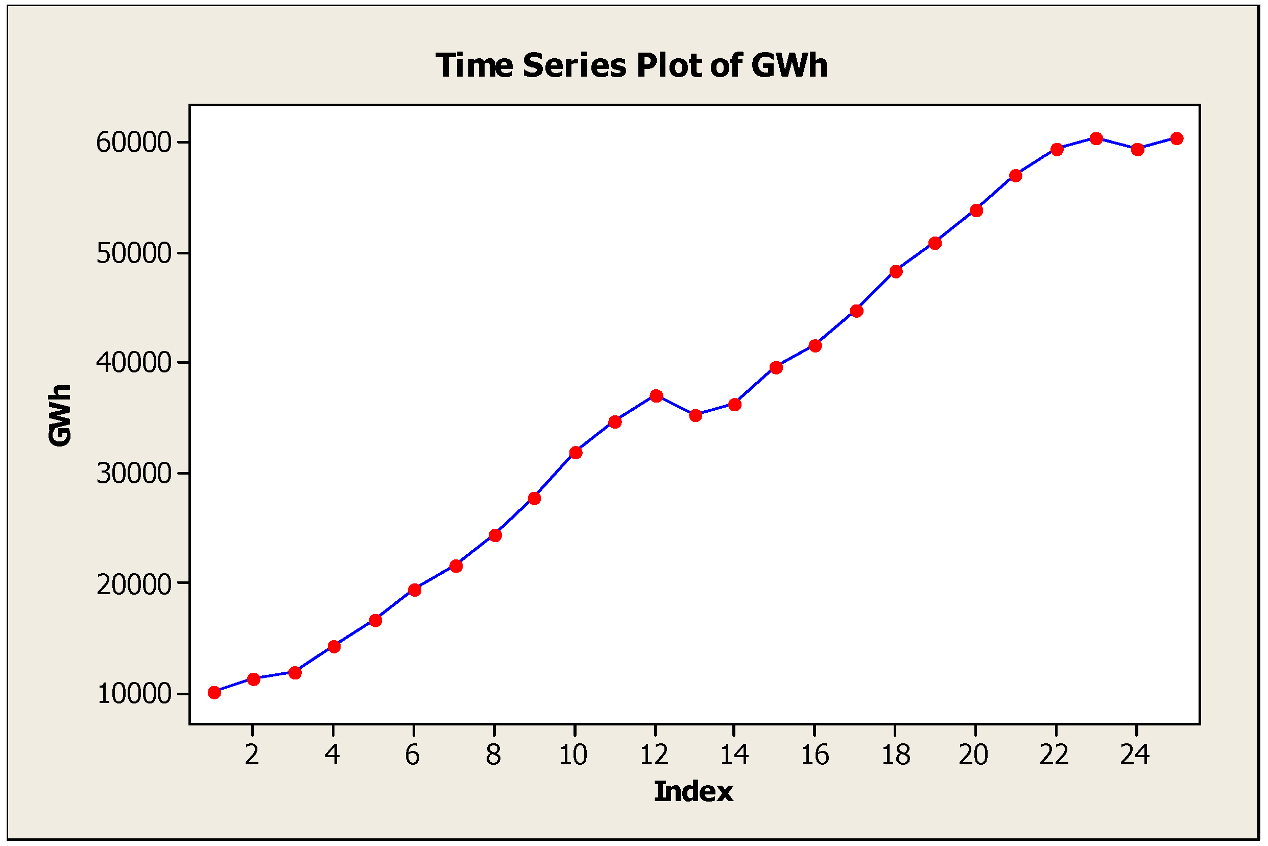
The order of an ARIMA model is normally identified in the form of (p, d, q), where p indicates the order of the autoregressive part, while d is for the amount of difference and q for the order of the moving average part. The electricity demand time series was plotted in Figure 1 in order to study the data structure before determining the appropriate ARIMA model. The plot showed that there was a constant growth rate of trend as time increased. However, no seasonality might exist in this case since there was no repeated pattern over time. Therefore, this set of data was not stationary and had a trend.

Figure 1. Time series plot of electricity demand.

Figure 1. Time series plot of electricity demand.

The concrete assumption of non-stationary data was supported by considering the correlogram of the demand (Figure 2) and it signified that the data was highly correlated at lag 1 and 2.

Figure 2. Correlogram of electricity demand.

Figure 2. Correlogram of electricity demand.

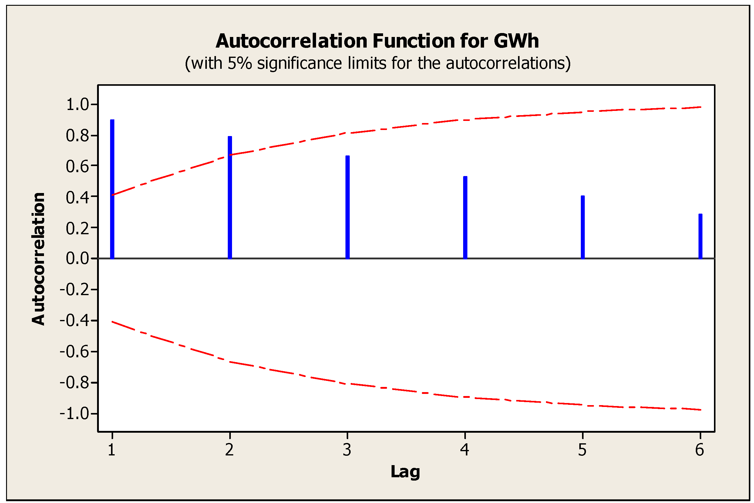
Therefore, since the correlation was embedded in the data, the ARIMA model was an interesting choice utilized to explain the data structure. A statistical package, StatGraphics Centurion version 14, was deployed to determine an ARIMA model and four different models were selected by the package based on their MAPEs (Table 2). The results indicated that the most appropriate ARIMA model to forecast the demand was ARIMA (0,2,2).

Table 2. Four different ARIMA models.

Model	MAPE
ARIMA (0,2,2)	2.80981
ARIMA (1,2,1)	3.02891
ARIMA (1,1,0)	3.34578
ARIMA (0,2,0)	3.30197

Table 2. Four different ARIMA models.

Model	MAPE
ARIMA (0,2,2)	2.80981
ARIMA (1,2,1)	3.02891
ARIMA (1,1,0)	3.34578
ARIMA (0,2,0)	3.30197

Equation (1) was rewritten as: where and . Let . The amount of p and q as well as β₁ in the ARIMA (p, 0, q) model: were calculated by a Box Jenkins method and AIC criterion where . Afterwards, let , and , the parameter of ARIMA (0,d,0) model: was estimated by applying the log Gaussian likelihood function as: where R = Covariance matrix of . The ARIMA (0,2,2) model coefficients are given in Table 3.

Table 3. Coefficients of ARIMA (0,2,2).

Parameter	Estimate
MA(1)	0.434155
MA(2)	0.488944

Table 3. Coefficients of ARIMA (0,2,2).

Parameter	Estimate
MA(1)	0.434155
MA(2)	0.488944

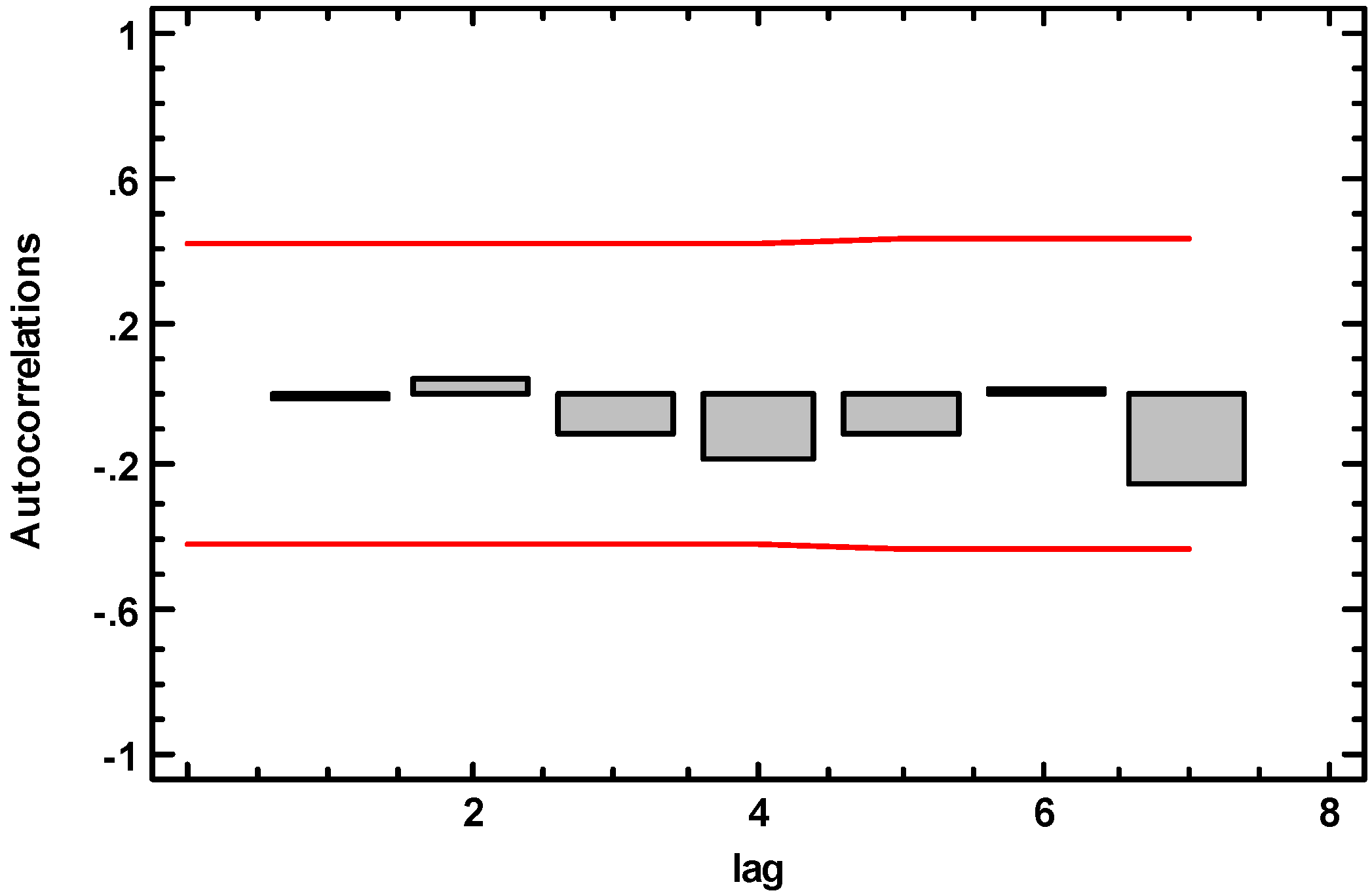
After the model was derived, the correlogram in Figure 3 was used to verify whether the residual was correlated or not. According to the correlogram, the correlations of each lag were not significant because they were still in the confidence interval.

Figure 3. Correlogram of the residual.

Figure 3. Correlogram of the residual.

3.2. Artificial Neural Network

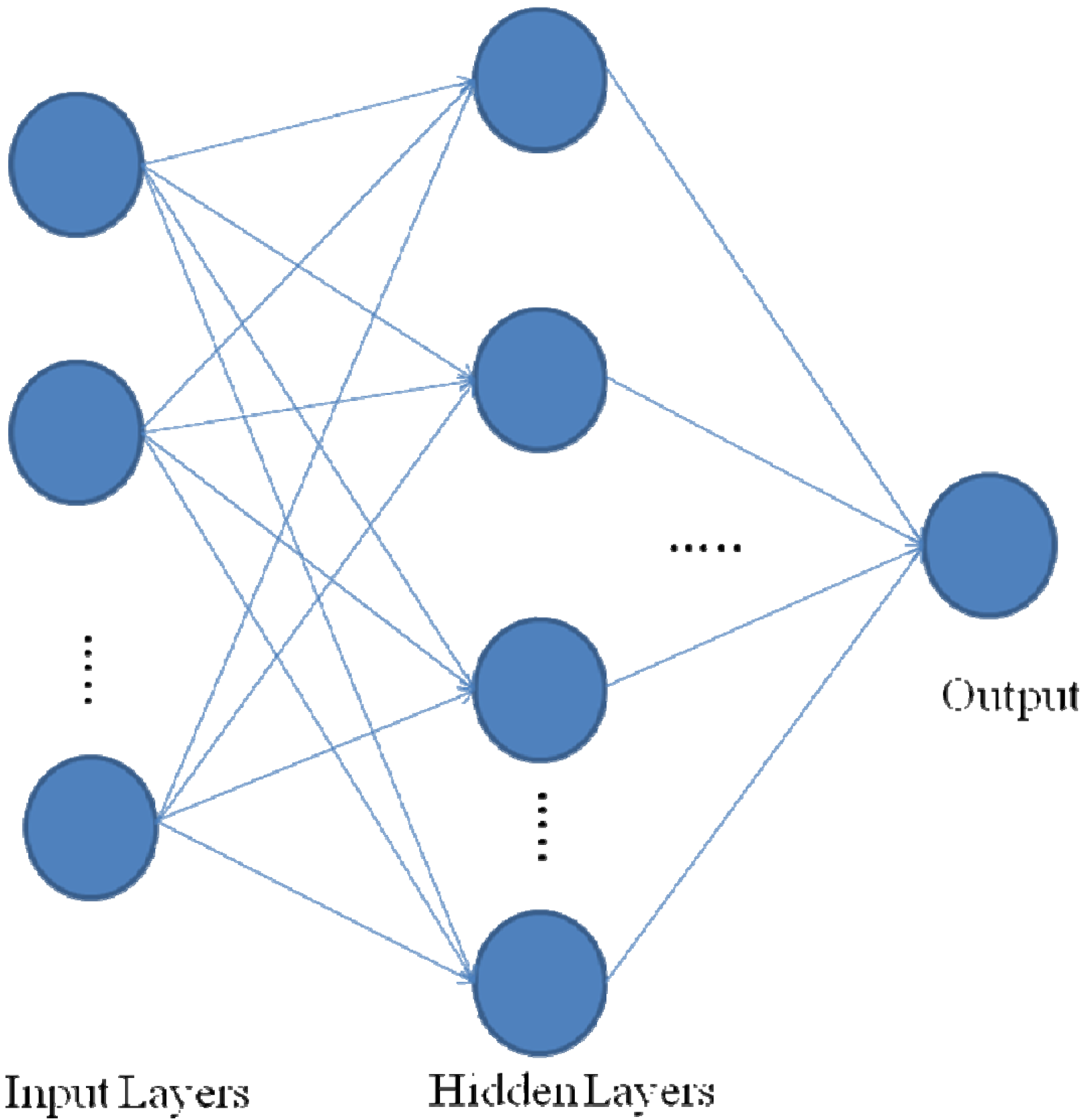
Basically, the neural architecture consists of three or more layers i.e., input layer, output layer and hidden layer, as shown in Figure 4.

Figure 4. The architecture of a neural network.

Figure 4. The architecture of a neural network.

The function of this network was described as follows:

(2)

where Y_j is the output of node j, f (.) is the transfer function, w_ij the connection weight between node j and node i in the lower layer and X_ij is the input signal from the node i in the lower layer to node j.

As shown in Equation (2), the network was a biased weighted sum of the inputs and passed the activation level through a transfer function to produce the output. The units of a network were arranged in the form of layered feedforward structure. In conclusion, any neural network was interpreted as a form of input-output model with the weights and free parameters of the model. For data analysis, the same set of data was divided into 25 cases with four input variables: population, SET index, GDP and Export, while the output variable was GWh. Two of the most popular neural network architectures, multilayer perceptrons (MLP) and radial basis function (RBF), were utilized for the regression purpose.

Normally, the ANN structure is based on the MLP architecture in which the number of layers and number of units in each layer are selected while the weights of networks and thresholds are set so as to minimize the prediction error. For RBF, its networks have a static Gaussian function as the nonlinearity for the hidden layer elements. The advantage of the RBF network was that it establishes the input to output map using local approximators which require few weights. For this reason, the networks were trained extremely fast and required fewer training samples.

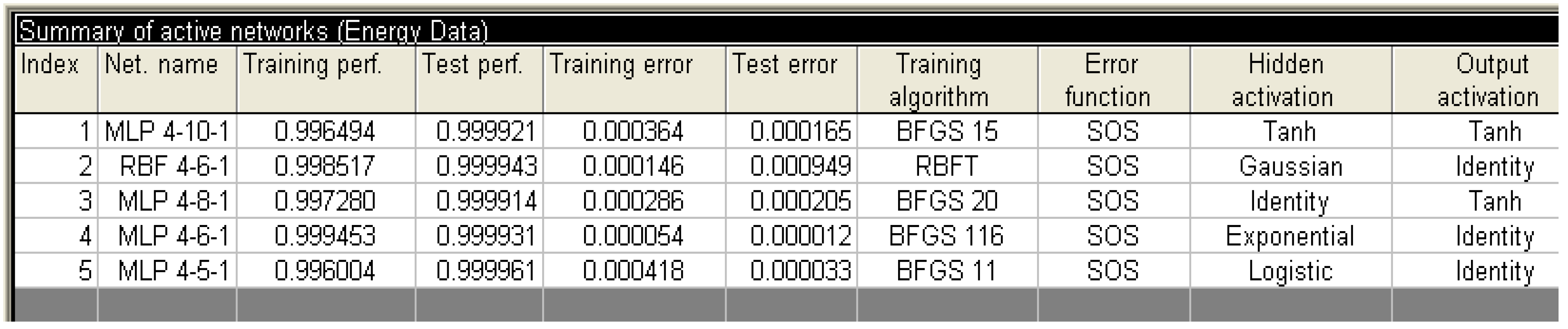
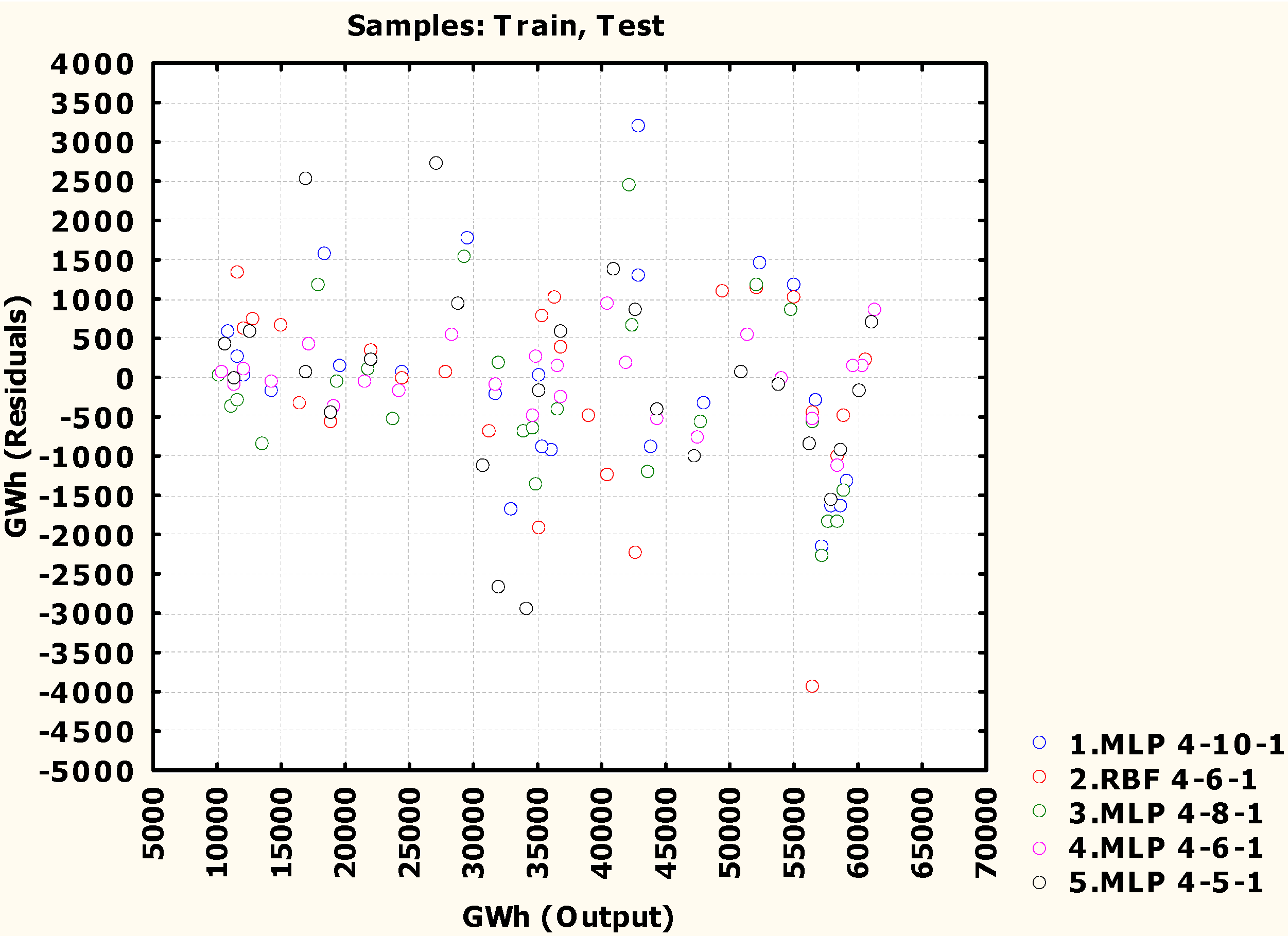
In this research, the amount of networks used to train was set at 200 while the top performing five networks were retained and shown in Table 4. STATISTICA version 8 was deployed to analyze the data and the results are illustrated in Figure 5. The results pointed out that the MLP network outperformed RBF when the number of hidden layers ranged from 5 to 10. The hidden neuron activation functions of the retained five networks were identity (the activation of the neuron was passed on directly as the output), Gaussian, Exponential and Logistic while the tangent hyperbolic (tanh) and identity functions were assigned to the output neuron activation functions. Moreover, the training algorithm of the MLP network employed to build the models was the Broyden-Fletcher-Goldfarb-Shanno (BFGS) algorithm with the number of cycles used to train the model ranging from 11 to 116 cycles. According to the MAPE in Table 4, MLP (4,6,1) model had the lowest error among all other models.

Table 4. Different neural networks and their MAPEs.

Model	MAPE
MLP (4,10,1)	2.770
RBF (4,6,1)	3.033
MLP (4,8,1)	2.598
MLP (4,6,1)	0.996
MLP (4,5,1)	3.2938

Table 4. Different neural networks and their MAPEs.

Model	MAPE
MLP (4,10,1)	2.770
RBF (4,6,1)	3.033
MLP (4,8,1)	2.598
MLP (4,6,1)	0.996
MLP (4,5,1)	3.2938

Figure 5. The ANN analysis results.

Figure 5. The ANN analysis results.

Due to Figure 6, the plot between errors and fitted values showed that the data was randomly scattered along the center line and there was no developed pattern like a funnel shape so the residual was uncorrelated with zero mean and constant variance.

Figure 6. Residuals vs. fitted plot.

Figure 6. Residuals vs. fitted plot.

3.3. Multiple Linear Regression

The general form of a multiple regression model was shown as follows:

(3)

where y_i is the dependent variable, x_.i is the independent variable, β_i is the regression coefficient of x_.i and ε_i is the random error. In order to construct the regression model, the independent variables (x_.i) were population, SET index, GDP and Export, while the dependent variable (y_i) was GWh. In order to estimate the coefficients of the model, the predicted response was shown in Equation (4):

(4)

The residuals between the observed and predicted responses were:

(5)

The sum square of residuals (SSE) was:

(6)

Then, taking the partial derivative of SSE with respect to each b_i and let it equal to zero. This yielded Equation (7):

(7)

n is the number of pairs (x₁, y₁), … , (x_n, y_n). The coefficients b₀, b₁, b₂, …, b_k were obtained by solving Equation (7). As a result, the regression equation was computed as follows:

GWh = − 91411 + 0.00170 × population + 0.00794 × GDP − 2.57 × SET Index + 0.00114 × Export

Figure 7. The normal probability plot of residuals.

Figure 7. The normal probability plot of residuals.

After the regression equation was derived, the model adequacy checking was performed. The normal probability plot in Figure 7 shows that the data points randomly formed a straight line so the errors were normally distributed. After the model was fitted to the data, the calculated error (MAPE) was 3.2604527.

4. Results

The errors from the above three methods are compared in Table 5. The results showed that the error minimization capability of the ANN model (0.996%) outperformed the other two approaches (2.80981% and 3.2604527%, respectively). However, the performance of ANN model was compared with those of the ARIMA and MLR models by utilizing two dependent samples tests. Therefore, the Wilcoxson signed-rank test and paired t-test were performed to assess the significant difference of the errors from these pairs: ANN:MLR and ANN:ARIMA.

Table 5. The comparison of errors from the three methods.

Model	MAPE
ARIMA (0,2,2)	2.80981
MLP (4,6,1)	0.996
MLR	3.2604527

Table 5. The comparison of errors from the three methods.

Model	MAPE
ARIMA (0,2,2)	2.80981
MLP (4,6,1)	0.996
MLR	3.2604527

The results of the Wilcoxson signed-rank test in Table 6 showed that there was no significant difference between the errors of ANN-MLR and ANN-ARIMA since their p-values (0.819095 and 0.784289 respectively) were much higher than 0.05. Due to Table 7, the paired t-test indicated the same results as the ones from signed-rank test.

Table 6. Wilcoxson signed-rank test for each pair of forecasting methods.

Pairs of Methods	p-value
ANN-MLR	0.819095
ANN-ARIMA	0.784289

Table 6. Wilcoxson signed-rank test for each pair of forecasting methods.

Pairs of Methods	p-value
ANN-MLR	0.819095
ANN-ARIMA	0.784289

Table 7. Paired t-test for each pair of forecasting methods.

Pairs of Methods	p-value
ANN-MLR	0.785697
ANN-ARIMA	0.927594

Table 7. Paired t-test for each pair of forecasting methods.

Pairs of Methods	p-value
ANN-MLR	0.785697
ANN-ARIMA	0.927594

5. Discussion

Although the artificial neural network has the best performance in this study (considering its MAPE solely), the matched pair tests did not indicate that there is a difference between the errors of each method. For this reason, the bottom line is that the decision should not depend on only one criterion to judge which method is the most appropriate one in each scenario. The critical issue in developing an ANN model is that its computation time is much higher than the other two because of its sophisticated architecture.

Moreover, its accuracy might be jeopardized from overfitting because of the limited number of available training cases. Another important issue is that it is quite difficult for practitioners to utilize and interpret an ANN model. On the other hand, the great advantage of using the ARIMA model is that it only needs the information regarding one variable to build a model. However, it will take time to choose the optimal coefficients, especially if the statistical package used lacks the capability of searching for the right coefficient. For MLR, although its accuracy is the lowest among all proposed methods, the algorithm is the simplest one. Additionally, it uses less calculation time to generate the regression model than the other two methods. As a result, users need to evaluate the trade-off between forecasting accuracy and limitation of the method before switching from traditional methods to ANN. This is an interesting issue since the important aspect of the forecasting is the principle of parsimony. If all models are equal, simple models will be preferred to complex models. For this reason, both ARIMA and MLR might be preferred to the ANN model since the structure of both methods is simpler than the one of ANN.

6. Conclusions

Three methodologies, ARIMA, ANN and MLR, were deployed to forecast the electricity demand in Thailand based on the historical data from 1986 to 2010. For the ARIMA approach, the results indicated that the ARIMA (0,2,2) was the best model to fit the historical data while the multilayer perceptrons (MLP) method was selected to use as the architecture for the ANN model. Four factors, i.e., amount of population, stock exchange index, GDP and amount of export were utilized to construct a MLR model. Although the results based on the error measurement showed that ANN model was superior to other approaches, paired tests pointed out that there was no significant difference among these errors. As a result, other factors should be utilized to determine the most appropriate model.

References

- Box, G.E.P.; Jenkins, G.M. Time Series Analysis: Forecasting and Control; Holden-Day: San Francisco, CA, USA, 1970; pp. 5–10. [Google Scholar]
- Montgomery, D.C.; Keats, J.B.; Runger, G.C.; Messina, W.S. Integrating statistical process control and engineering process control. J. Qual. Technol. 1994, 26, 79–87. [Google Scholar]
- Box, G.E.P.; Luceno, A. Statistical Control by Monitoring and Feedback Adjustment; John Wiley & Sons: New York, NY, USA, 1997. [Google Scholar]
- Ediger, V.S.; Akar, S. ARIMA forecasting of primary energy demand by fuel in Turkey. Energy Policy 2007, 35, 1701–1708. [Google Scholar] [CrossRef]
- Abdel-Aal, R.E.; Al-Garni, A.Z. Forecasting monthly electric energy consumption in eastern saudi arabia using univariate time-series analysis. Energy 1997, 22, 1059–1069. [Google Scholar] [CrossRef]
- Zhou, P.; Ang, B.W.; Poh, K.L. A trigonometry grey prediction approach to forecasting electricity demand. Energy 2006, 31, 2839–2847. [Google Scholar] [CrossRef]
- Cho, M.Y.; Hwang, J.C.; Chen, C.S. Customer Short Term Load Forecasting by Using ARIMA Transfer Function Model. In Proceedings of the International Conference on Energy Management and Power Delivery, EMPD’95, Singapore, 20–23 November 1995; pp. 317–322.
- Hsu, C.-C.; Chen, C.-Y. Regional load forecasting in Taiwan-applications of artificial neural networks. Energy Convers. Manag. 2003, 44, 1941–1949. [Google Scholar] [CrossRef]
- Catalao, J.P.S.; Mariano, S.J.P.S.; Mendes, V.M.F.; Ferreira, L.A.F.M. Short-term electricity prices forecasting in a competitive market: A neural network approach. Electr. Power Syst. Res. 2007, 77, 1297–1304. [Google Scholar] [CrossRef]
- Bakirtzis, A.G.; Petridis, V.; Klartzis, S.J.; Alexladis, M.C. A neural network short term load forecasting model for the greek power system. IEEE Trans. Power Syst. 1996, 11, 858–863. [Google Scholar] [CrossRef]
- Mohamed, Z.; Bodger, P. Forecasting electricity consumption in New Zealand using economic and demographic variables. Energy 2005, 30, 1833–1843. [Google Scholar] [CrossRef]
- Azadeh, A.; Ghaderi, S.F.; Tarverdian, S.; Saberi, M. Intergraion of artificial neural networks and genetic algorithm to predict electrical energy consumption. Appl. Math. Comput. 2007, 186, 1731–1741. [Google Scholar] [CrossRef]
- Azadeh, A.; Ghaderi, S.F.; Sohrabkhani, S. A simulated-based neural network algorithm for forecasting electrical energy consumption in Iran. Energy Policy 2008, 36, 2637–2644. [Google Scholar] [CrossRef]
- Hong, W.-C. Electric load forecasting by support vector model. Appl. Math. Model. 2009, 33, 2444–2454. [Google Scholar] [CrossRef]
- Ekonomou, L. Greek long-term energy consumption prediction using artificial neural networks. Energy 2010, 35, 512–517. [Google Scholar] [CrossRef]
- Pappas, S.S.; Ekonomou, L.; Karamousantas, D.C.; Chatzarakis, G.E.; Katsikas, S.K.; Liatsis, P. Electricity demand loads modeling using autoregressive moving average (ARIMA) models. Energy 2008, 33, 1353–1360. [Google Scholar] [CrossRef]
© 2011 by the authors; licensee MDPI, Basel, Switzerland. This article is an open access article distributed under the terms and conditions of the Creative Commons Attribution license (http://creativecommons.org/licenses/by/3.0/).
Share and Cite
MDPI and ACS Style
Kandananond, K. Forecasting Electricity Demand in Thailand with an Artificial Neural Network Approach. Energies 2011, 4, 1246-1257. https://doi.org/10.3390/en4081246
AMA Style
Kandananond K. Forecasting Electricity Demand in Thailand with an Artificial Neural Network Approach. Energies. 2011; 4(8):1246-1257. https://doi.org/10.3390/en4081246
Chicago/Turabian StyleKandananond, Karin. 2011. "Forecasting Electricity Demand in Thailand with an Artificial Neural Network Approach" Energies 4, no. 8: 1246-1257. https://doi.org/10.3390/en4081246