Temporal and Spatial Analysis of Integrated Energy and Environment Efficiency in China Based on a Green GDP Index

Abstract
:1. Introduction
2. Green GDP Index
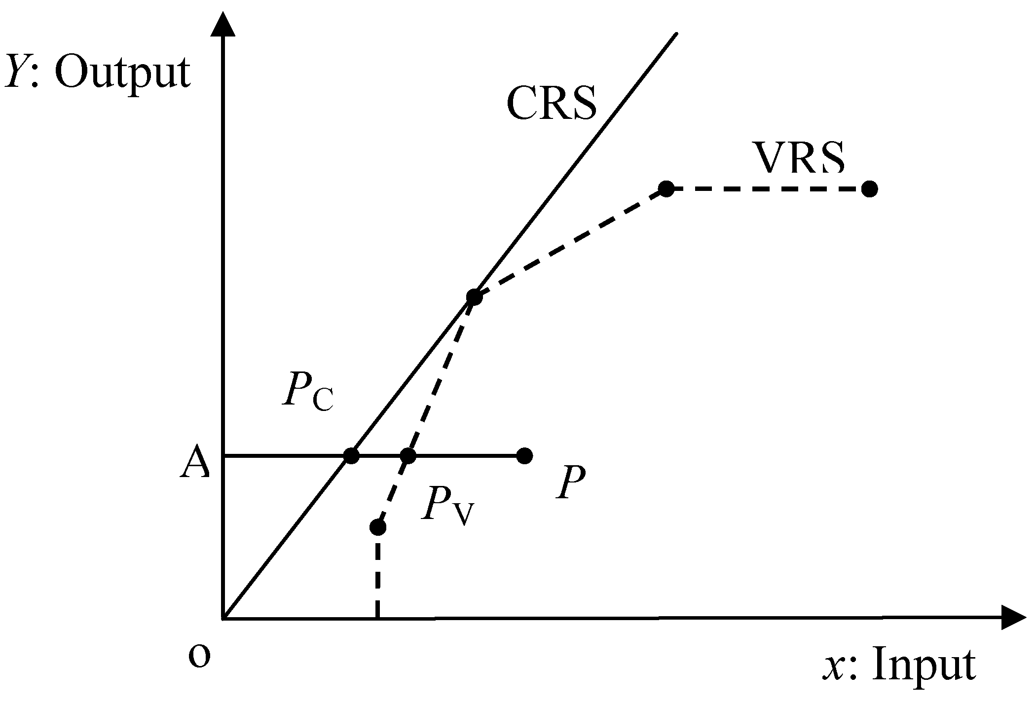
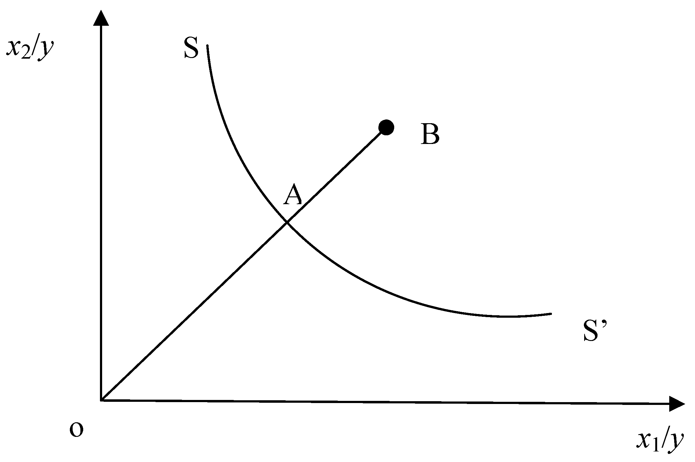
2.1. DEA Model

2.2. Malmquist Index
2.3. Data Sources
3. Results and Discussion
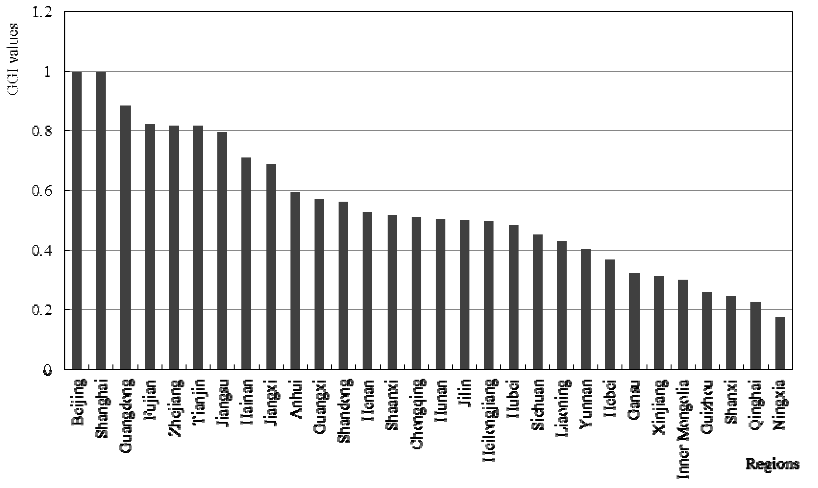
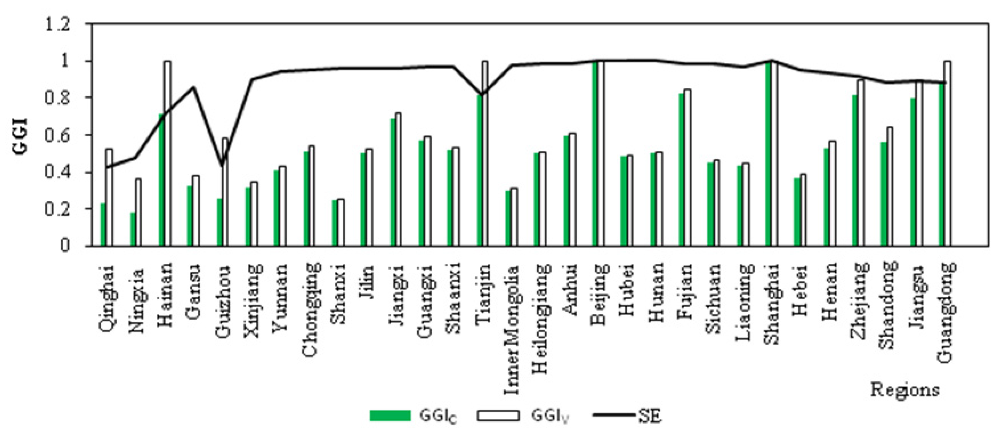
3.1. Regional Discrepancies

| Regions (DMUs) | GGIC | GGIV | SE | Stage | Regions (DMUs) | GGIC | GGIV | SE | Stage |
|---|---|---|---|---|---|---|---|---|---|
| Beijing | 1 | 1 | 1 | constant | Hunan | 0.504 | 0.506 | 0.996 | decreasing |
| Shanghai | 1 | 1 | 1 | constant | Jilin | 0.501 | 0.522 | 0.958 | increasing |
| Guangdong | 0.885 | 1 | 0.885 | decreasing | Heilongjiang | 0.498 | 0.506 | 0.984 | increasing |
| Fujian | 0.825 | 0.841 | 0.981 | decreasing | Hubei | 0.485 | 0.486 | 0.998 | decreasing |
| Zhejiang | 0.818 | 0.892 | 0.917 | decreasing | Sichuan | 0.453 | 0.463 | 0.98 | decreasing |
| Tianjin | 0.817 | 1 | 0.817 | increasing | Liaoning | 0.43 | 0.446 | 0.964 | increasing |
| Jiangsu | 0.796 | 0.892 | 0.892 | decreasing | Yunnan | 0.406 | 0.431 | 0.941 | decreasing |
| Hainan | 0.713 | 1 | 0.713 | increasing | Hebei | 0.37 | 0.391 | 0.947 | decreasing |
| Jiangxi | 0.689 | 0.716 | 0.962 | increasing | Gansu | 0.325 | 0.379 | 0.857 | increasing |
| Anhui | 0.596 | 0.605 | 0.985 | increasing | Xinjiang | 0.314 | 0.348 | 0.9 | increasing |
| Guangxi | 0.573 | 0.595 | 0.963 | increasing | Inner Mongolia | 0.302 | 0.31 | 0.975 | increasing |
| Shandong | 0.564 | 0.641 | 0.881 | decreasing | Guizhou | 0.258 | 0.584 | 0.441 | increasing |
| Henan | 0.529 | 0.566 | 0.935 | decreasing | Shanxi | 0.247 | 0.257 | 0.958 | increasing |
| Shaanxi | 0.517 | 0.536 | 0.965 | increasing | Qinghai | 0.226 | 0.525 | 0.43 | increasing |
| Chongqing | 0.513 | 0.539 | 0.951 | increasing | Ningxia | 0.175 | 0.364 | 0.481 | increasing |
| Average | 0.544 | 0.611 | 0.889 | ||||||


3.2. GGI Trends
| Year | 2006 | 2007 | 2008 | 2009 | Average | |
|---|---|---|---|---|---|---|
| DMUs | ||||||
| Beijing | 1.491 | 1.194 | 1.355 | 1.072 | 1.268 | |
| Tianjin | 1.116 | 1.073 | 1.126 | 1.057 | 1.093 | |
| Hebei | 1.032 | 1.042 | 1.068 | 1.053 | 1.049 | |
| Shanxi | 1.02 | 1.047 | 1.08 | 1.062 | 1.052 | |
| Inner Mongolia | 1.026 | 1.047 | 1.068 | 1.074 | 1.053 | |
| Liaoning | 1.037 | 1.042 | 1.054 | 1.053 | 1.047 | |
| Jilin | 1.035 | 1.046 | 1.053 | 1.063 | 1.049 | |
| Heilongjiang | 1.034 | 1.043 | 1.05 | 1.059 | 1.047 | |
| Shanghai | 1.106 | 1.247 | 1.153 | 1.143 | 1.161 | |
| Jiangsu | 1.036 | 1.044 | 1.062 | 1.054 | 1.049 | |
| Zhejiang | 1.037 | 1.044 | 1.058 | 1.057 | 1.049 | |
| Anhui | 1.031 | 1.043 | 1.047 | 1.057 | 1.044 | |
| Fujian | 1.041 | 1.098 | 1.076 | 1.037 | 1.062 | |
| Jiangxi | 1.033 | 1.044 | 1.063 | 1.047 | 1.047 | |
| Shandong | 1.036 | 1.048 | 1.069 | 1.055 | 1.052 | |
| Henan | 1.031 | 1.043 | 1.054 | 1.064 | 1.048 | |
| Hubei | 1.033 | 1.042 | 1.072 | 1.061 | 1.052 | |
| Hunan | 1.035 | 1.046 | 1.072 | 1.053 | 1.051 | |
| Guangdong | 1.03 | 1.033 | 1.045 | 1.043 | 1.038 | |
| Jiangxi | 1.026 | 1.034 | 1.041 | 1.046 | 1.037 | |
| Hainan | 1.011 | 1.008 | 1.027 | 1.028 | 1.019 | |
| Chongqing | 1.035 | 1.046 | 1.052 | 1.058 | 1.048 | |
| Sichuan | 1.033 | 1.046 | 1.042 | 1.062 | 1.046 | |
| Guizhou | 1.031 | 1.042 | 1.068 | 1.041 | 1.046 | |
| Yunnan | 1.015 | 1.041 | 1.05 | 1.048 | 1.039 | |
| Shaanxi | 1.035 | 1.048 | 1.063 | 1.047 | 1.048 | |
| Gansu | 1.027 | 1.043 | 1.053 | 1.073 | 1.049 | |
| Qinghai | 0.994 | 1.031 | 1.043 | 1.069 | 1.034 | |
| Ningxia | 1.01 | 1.037 | 1.073 | 1.064 | 1.046 | |
| Xinjiang | 1.011 | 1.032 | 1.032 | 1.015 | 1.022 | |
| Average | 1.046 | 1.055 | 1.071 | 1.057 | 1.057 | |
| Year | GDP (1 billion yuan) | Energy Intensity (tce/10,000 yuan) | SO2 (10,000 ton) | Soot (10,000 ton) | Dust (10,000 ton) | COD (10,000 ton) | Ammonia Nitrogen (10,000 ton) |
|---|---|---|---|---|---|---|---|
| 2006 | 20,838.10 | 1.24 | 2234.8 | 864.5 | 808.4 | 541.5 | 42.5 |
| 2007 | 23,789.28 | 1.18 | 2140 | 771.1 | 698.7 | 511.1 | 34.1 |
| 2008 | 26,081.29 | 1.12 | 1991.4 | 670.7 | 584.9 | 457.6 | 29.7 |
| 2009 | 28,457.20 | 1.08 | 1865.9 | 604.4 | 523.6 | 439.7 | 27.4 |
| Average | 24,791.47 | 1.155 | 2058.025 | 727.675 | 653.9 | 487.475 | 33.425 |
| Change rate | 36.56% | 12.90% | 16.51% | 30.09% | 35.23% | 18.80% | 35.53% |
| Region | Change in Relative Green Index | Change in Green Frontier | Change in Pure Green Index | Change in Scale Effect | Change in Green Index |
|---|---|---|---|---|---|
| Beijing | 1 | 1.268 | 1 | 1 | 1.268 |
| Tianjin | 1.011 | 1.081 | 1.051 | 0.962 | 1.093 |
| Hebei | 0.981 | 1.069 | 0.994 | 0.987 | 1.049 |
| Shanxi | 0.984 | 1.069 | 0.991 | 0.993 | 1.052 |
| Inner Mongolia | 0.985 | 1.069 | 0.987 | 0.998 | 1.053 |
| Liaoning | 0.979 | 1.069 | 0.988 | 0.991 | 1.047 |
| Jilin | 0.981 | 1.069 | 0.987 | 0.995 | 1.049 |
| Heilongjiang | 0.979 | 1.069 | 0.981 | 0.998 | 1.047 |
| Shanghai | 1 | 1.161 | 1 | 1 | 1.161 |
| Jiangsu | 0.981 | 1.069 | 1.009 | 0.972 | 1.049 |
| Zhejiang | 0.981 | 1.069 | 1.002 | 0.979 | 1.049 |
| Anhui | 0.977 | 1.069 | 0.979 | 0.998 | 1.044 |
| Fujian | 0.994 | 1.069 | 0.998 | 0.995 | 1.062 |
| Jiangxi | 0.979 | 1.069 | 0.985 | 0.994 | 1.047 |
| Shandong | 0.984 | 1.069 | 1.011 | 0.973 | 1.052 |
| Henan | 0.98 | 1.069 | 0.996 | 0.984 | 1.048 |
| Hubei | 0.984 | 1.069 | 0.984 | 1 | 1.052 |
| Hunan | 0.984 | 1.069 | 0.984 | 0.999 | 1.051 |
| Guangdong | 0.971 | 1.069 | 1 | 0.971 | 1.038 |
| Guangxi | 0.97 | 1.069 | 0.975 | 0.995 | 1.037 |
| Hainan | 0.953 | 1.069 | 1 | 0.953 | 1.019 |
| Chongqing | 0.98 | 1.069 | 0.987 | 0.993 | 1.048 |
| Sichuan | 0.978 | 1.069 | 0.983 | 0.995 | 1.046 |
| Guizhou | 0.978 | 1.069 | 1.035 | 0.945 | 1.046 |
| Yunnan | 0.972 | 1.069 | 0.981 | 0.991 | 1.039 |
| Shaanxi | 0.981 | 1.069 | 0.985 | 0.996 | 1.048 |
| Gansu | 0.981 | 1.069 | 1.005 | 0.976 | 1.049 |
| Qinghai | 0.967 | 1.069 | 1.016 | 0.952 | 1.034 |
| Ningxia | 0.978 | 1.069 | 1.029 | 0.95 | 1.046 |
| Xinjiang | 0.956 | 1.069 | 0.973 | 0.983 | 1.022 |
| Average | 0.980 | 1.079 | 0.996 | 0.984 | 1.057 |
| Object | Studying Period | Production Efficiency | References |
|---|---|---|---|
| Integrated energy and environmental efficiency of China | 2009 | 54.4 | This paper |
| Industrial energy efficiency of Chinese industrial system | 2006 | 47.67 | [16] |
| Resource efficiency of Chinese industrial system | 2004 | 49.8 | [20] |
| Environmental efficiency of Chinese industrial system | 2004 | 55.53 | [20] |
| Resource efficiency of China | 2006 | 42.15 | [25] |
4. Conclusions
- (1)
- The integrated energy and environment efficiencies of these regions vary greatly. Beijing and Shanghai have the lowest energy consumptions and environment pollutions during the GDP growth process, with a green index of 1. The green indexes of the developed eastern regions like Guangdong, Fujian, Zhejiang, Tianjin, Jiangsu and Hainan are in the top ranking, while those of the northeastern and middle regions relatively fall behind. There are severe energy and environment problems in the northwest and south areas such as Ningxia, Qinghai, Shanxi, Guizhou and Inner Mongolia, which are far from the green frontier, with GGIs all being below 0.3.
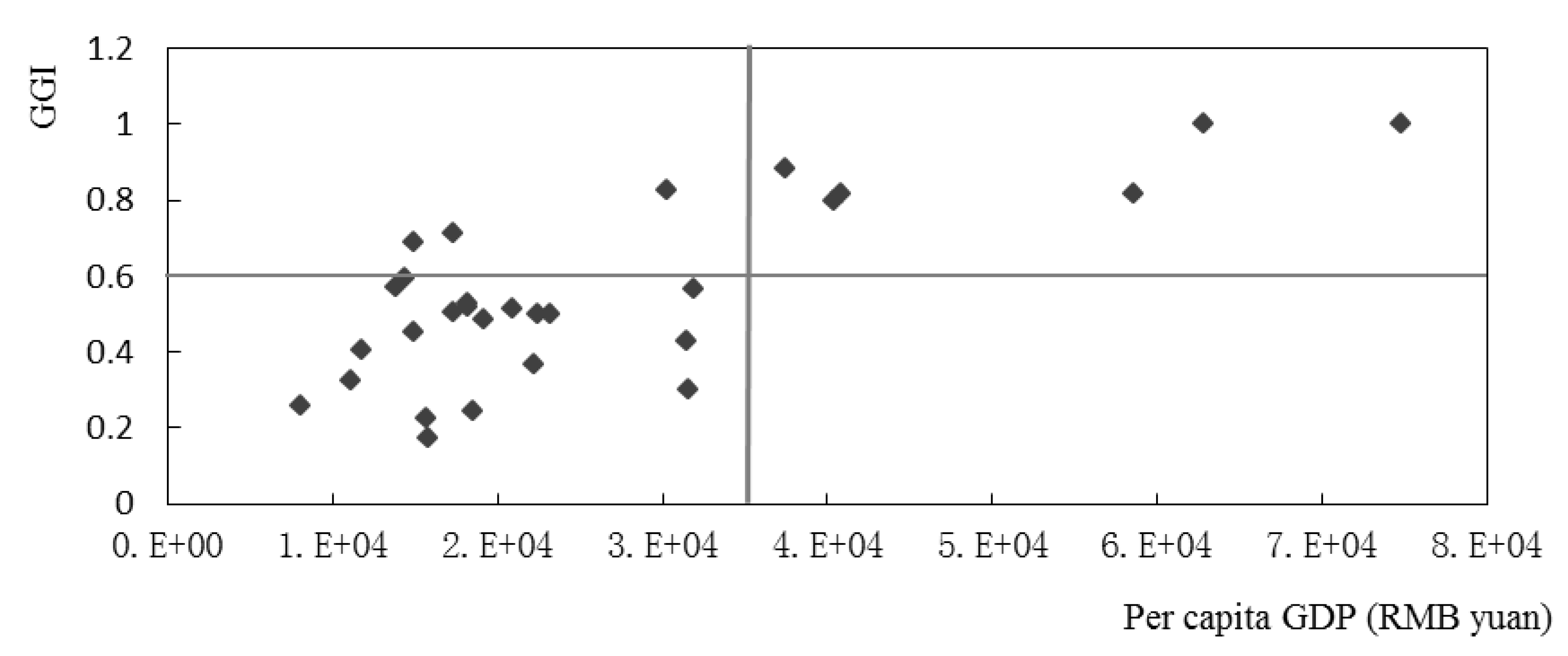
- (2)
- The provincial differences between GGIs reflect the specific development modes, which depend on the varying level of development of each area. There is an obvious positive correlation between the green index and per capita GDP, with the correlation coefficient being 0.75. Almost all the green indexes are above 0.6 in the regions with per capita GDP of more than 0.35 million yuan, while the green indexes are below 0.6 in the regions whose per capita GDP are below 0.35 million yuan, indicating that dependence of economic growth on energy consumption and environmental pollution will gradually decrease.
- (3)
- Increases of different degree in GGIs of all DMUs are found from 2006 to 2008, which represent the great achievements of the Energy Conservation & Emission Reduction movement in China. However, GGIs of these provinces have not converged to the green frontier, showing a more or less divergent trend.
Acknowledgements
References
- Chen, B.; Chen, G.Q. Ecological footprint accounting based on emergy—A case study of the Chinese society. Ecol. Model 2006, 198, 101–114. [Google Scholar] [CrossRef]
- Chen, B.; Chen, G.Q.; Yang, Z.F.; Jiang, M.M. Ecological footprint accounting for energy and resource in China. Energy Policy 2007, 35, 1599–1609. [Google Scholar] [CrossRef]
- Chen, B.; Chen, G.Q. Modified ecological footprint accounting and analysis based on embodied exergy—a case study of the Chinese society 1981–2001. Ecol. Econ. 2007, 61, 355–376. [Google Scholar] [CrossRef]
- Zhang, L.X.; Chen, B.; Yang, Z.F.; Chen, G.Q.; Jiang, M.M.; Liu, G.Y. Comparison of typical mega cities in China using emergy synthesis. Commun. Nonlinear Sci. Numer. Simul. 2009, 14, 2827–2836. [Google Scholar] [CrossRef]
- Chen, B.; Chen, G.Q. Resource analysis of the Chinese society 1980–2002 based on exergy—Part 2: Renewable energy sources and forest. Energy Policy 2007, 35, 2051–2064. [Google Scholar] [CrossRef]
- Chen, B.; Chen, G.Q. Resource analysis of the Chinese society 1980–2002 based on energy—Part 5: Resource structure and intensity. Energy Policy 2007, 35, 2087–2095. [Google Scholar] [CrossRef]
- Chen, Z.M.; Chen, G.Q.; Zhou, J.B.; Jiang, M.M.; Chen, B. Ecological input–output modeling for embodied resources and emissions in Chinese economy 2005. Commun. Nonlinear Sci. Numer. Simul. 2010, 15, 1942–1965. [Google Scholar] [CrossRef]
- Zhou, P.; Ang, B.W.; Poh, K.L. A survey of data envelopment analysis in energy and environmental studies. Eur. J. Oper. Res. 2008, 189, 1–18. [Google Scholar] [CrossRef]
- Farrell, M.J. The Measurement of productive efficiency. J. R. Stat. Soc. A Stat. Part 3 1957, 20, 253–290. [Google Scholar] [CrossRef]
- Burley, H. Productive efficiency in U.S. manufacturing: A linear programming approach. Rev. Econ. Stat. 1980, 11, 619–622. [Google Scholar]
- Banker, R.D.; Charnes, A.; Cooper, W.W. Some models for estimating technical and scale inefficiencies in data envelopment analysis. Manag. Sci. 1984, 30, 1078–1092. [Google Scholar] [CrossRef]
- Färe, R.; Grosskopf, S.; Norris, M.; Zhang, Z. Productivity Growth, Technical progress, and efficiency changes in industrialised countries. Am. Econ. Rev. 1994, 84, 66–83. [Google Scholar]
- Lovell, C.A.K. Linear programming approaches to the measurement and analysis of productive efficiency. Top 1994, 2, 175–248. [Google Scholar] [CrossRef]
- Coelli, T.J. A multi-stage methodology for the solution of orientated DEA models. Oper. Res. Lett. 1998, 23, 143–149. [Google Scholar] [CrossRef]
- Mousavi-Avval, S.H.; Rafiee, S.; Jafari, A.; Mohammadi, A. Improving energy use efficiency of canola production using data envelopment analysis (DEA) approach. Energy 2011, 36, 2765–2772. [Google Scholar] [CrossRef]
- Shi, G.M.; Bi, J.; Wang, J.N. Chinese regional industrial energy efficiency evaluation based on a DEA model of fixing non-energy inputs. Energy Policy 2010, 38, 6172–6179. [Google Scholar] [CrossRef]
- Ramanathan, R. A holistic approach to compare energy efficiencies of different transport modes. Energy Policy 2000, 28, 743–747. [Google Scholar] [CrossRef]
- Färe, R.; Grosskopf, S.; Lovell, C.A.K.; Pasurka, C. Multilateral productivity comparisons when some outputs are undesirable: a nonparametric approach. Rev. Econ. Statis. 1989, 71, 90–98. [Google Scholar] [CrossRef]
- Tyteca, D. Linear programming models for the measurement of environmental performance of firms-concepts and empirical results. J. Prod. Anal. 1997, 8, 183–197. [Google Scholar] [CrossRef]
- Zhang, B.; Bi, J.; Fan, Z.Y.; Yuan, Z. W.; Ge, J.J. Eco-efficiency analysis of industrial system in China: A data envelopment analysis approach. Ecol. Econ. 2008, 68, 306–316. [Google Scholar] [CrossRef]
- Sueyoshi, T.; Goto, M.; Ueno, T. Performance analysis of US coal-fired power plants by measuring three DEA efficiencies. Energy Policy 2010, 38, 1675–1688. [Google Scholar] [CrossRef]
- Zhou, P.; Ang, B.W.; Han, J.Y. Total factor carbon emission performance: a Malmquist index analysis. Energy Econ. 2010, 32, 194–201. [Google Scholar] [CrossRef]
- Guo, X.D.; Zhu, L.; Fan, Y.; Xie, B.C. Evaluation of potential reductions in carbon emissions in Chinese provinces based on environmental DEA. Energy Policy 2011, 39, 2352–2360. [Google Scholar] [CrossRef]
- Hall, B.; Kerr, M.L. 1991–1992 Green Index: A State-by-State Guide to the Nation’s Environmental Health; Island Press: Washington, DC, USA, 1991. [Google Scholar]
- Bian, Y.W.; Yang, F. Resource and environment efficiency analysis of provinces in China: A DEA approach based on Shannon’s entropy. Energy Policy 2010, 38, 1909–1917. [Google Scholar] [CrossRef]
- China Energy Statistical Yearbook 2010; China Statistics Press: Beijing, China, 2010.
- China Environment Statistical Yearbook 2010; China Statistics Press: Beijing, China, 2010.
© 2011 by the authors; licensee MDPI, Basel, Switzerland. This article is an open access article distributed under the terms and conditions of the Creative Commons Attribution license (http://creativecommons.org/licenses/by/3.0/).
Share and Cite
Lin, W.; Yang, J.; Chen, B. Temporal and Spatial Analysis of Integrated Energy and Environment Efficiency in China Based on a Green GDP Index. Energies 2011, 4, 1376-1390. https://doi.org/10.3390/en4091376
Lin W, Yang J, Chen B. Temporal and Spatial Analysis of Integrated Energy and Environment Efficiency in China Based on a Green GDP Index. Energies. 2011; 4(9):1376-1390. https://doi.org/10.3390/en4091376
Chicago/Turabian StyleLin, Weibin, Jin Yang, and Bin Chen. 2011. "Temporal and Spatial Analysis of Integrated Energy and Environment Efficiency in China Based on a Green GDP Index" Energies 4, no. 9: 1376-1390. https://doi.org/10.3390/en4091376