Steady State Assessment of Shunt Compensated EHV Insulated Cables by Means of Multiconductor Cell Analysis (MCA)

Abstract

The author has already presented some papers which allow studying cable systems by means of the multiconductor cell analysis (MCA). This method considers the cable system in its real asymmetry without simplified and approximated hypotheses. The multiconductor matrix procedure based on the use of admittance matrices, which account for the line cells (with earth return currents), different types of screen bonding, possible multiple circuits (single and double circuit or more), allows predicting the steady-state regime of any cable system. In the previous papers, these matrix algorithms have been presented with reference to a short extra-high voltage (EHV) double-circuit cross-bonded (CB) underground cable (UGC) system. Since the cable link was short, the shunt reactive compensation was not necessary and consequently not considered. In this paper the procedure is generalized in order to take into account three single-phase (or also one three-phase) reactors installed at the cable ends or also at intermediate locations.

1. Introduction

Insulated cables constitute complex cases of multiconductor systems, which cannot be studied in detail by means of a simplified single-phase equivalent circuit. In electrical system research, the multiconductor theory is used in several situations, e.g., analysis of electromagnetic interferences between systems of different kind. Obviously, the modelling used for the abovementioned electromagnetic compatibility studies cannot be applied to multiconductor analysis inside a unique power system where besides the overhead lines, there are also UGCs with their metallic screens. Hence it is easy to understand how, by considering the physical reality of the power networks, it can be questionable to assume purely three-phase configurations and perfectly symmetrical ones, so to use the three sequence modelling. In many cases, multiconductor analysis becomes necessary, since it allows one to achieve great precision results, thus offering a powerful tool in order to validate approximated and simplified computation methods. The whole exposition of the MCA can be found in [1,2] or, with a more didactical approach, in a book [3].

2. Brief Recalls to Shunt Compensation Features

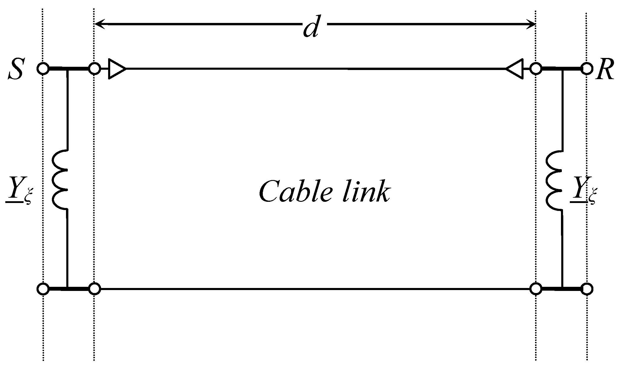
It is absolutely known that the kilometric cable capacitive susceptance has such a high value to determine (chiefly with great lengths, voltages and sections) in the network steady state and transient regimes that it could become very severe or even unacceptable, unless a suitable shunt compensation is adopted. The compensation of the uniformly distributed cable capacitive susceptance would theoretically require the insertion of uniformly distributed inductive susceptance. Since this is merely theoretical, the compensation is lumped. 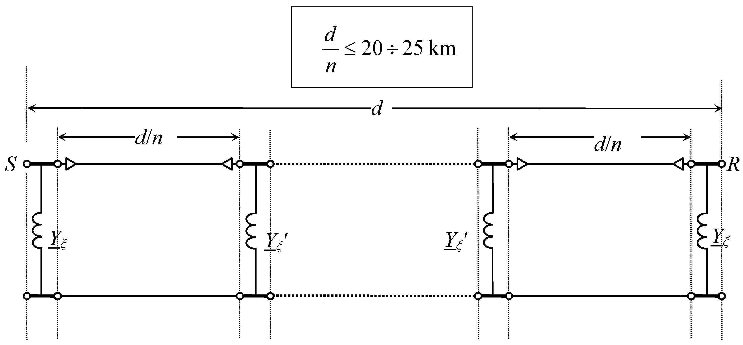In order to give the reader some brief context, the lumped compensation can be performed both at the two ends (see Figure 1) or also at intermediate locations (see Figure 2). If the cable to be compensated has a length greater than $20÷25$ km it is suitable to also install shunt reactors at intermediate sections, provided with individuating n sections within the limits shown in Figure 2. The value Y_ξ depends upon the shunt compensation degree, whose value can be computed by means of the criteria developed in the next subsection, which refer to the single-phase circuit. The value of Y_ξ is obviously different depending upon these two different situations. In case of Figure 1, Y_ξ can be computed as in Equation (1):

$${\underset{¯}{Y}}_{\xi }=-j\omega c{\xi }_{sh}\frac{d}{2}$$

(1)

where:

• ξ_sh = shunt compensation degree;
• c = UGC kilometric capacitance (F/km);
• d = cable line length (km).

Figure 1. Lumped shunt compensation at the two ends.

Figure 1. Lumped shunt compensation at the two ends.

Figure 2. Lumped shunt compensation at the ends and at intermediate locations.

Figure 2. Lumped shunt compensation at the ends and at intermediate locations.

The computation of Y_ξ and Y_ξ' in case of lumped compensation also at intermediate locations (see Figure 2) becomes:

$${{\underset{¯}{Y}}^{\prime }}_{\xi }=2{\underset{¯}{Y}}_{\xi }=-j\omega c{\xi }_{sh}\frac{d}{n}$$

(2)

The Determination of Shunt Compensation Degree by Means of Single-Phase Circuit

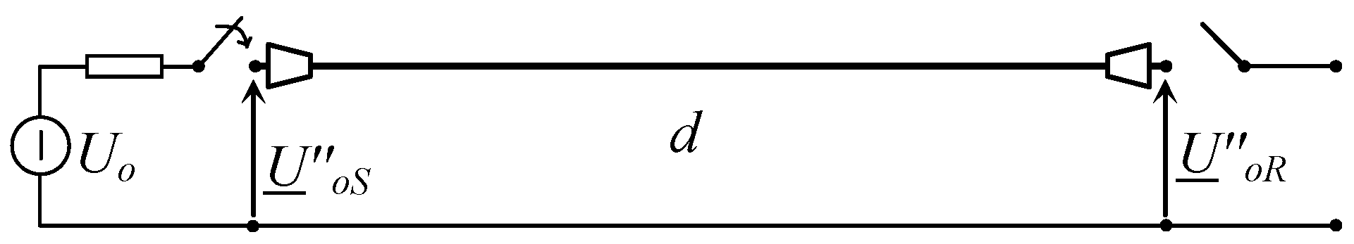
It is worth remembering that during network operation, very frequently recurring events of the greatest concern are the energization and de-energization of a no-load line since they are always necessary to prepare the operating structure of the grid. The simple sketch of Figure 3 shows the switch-on of the circuit breaker in S in order to energize the cable and serves as a first, not complete but meaningful approach devoted to highlight the limit conditions for line energisation at no-load. In a generic network, the power supply in S can be modelled as an equivalent generator which is characterized by its electromotive force U_o (assumed U_o = 230 kV) and the short-circuit subtransient impedance Z'' (for simplicity purely inductive Z'' = jX'').

Figure 3. No load energization at port S.

Figure 3. No load energization at port S.

The magnitude of no-load power frequency sub-transient voltage ${\underset{¯}{U}}_{oR}^{″}$ at R, due to the closing at S, constitutes a reference (“indicial” value) to foresee the peak value of switching surges due to subsequent evolution of the phenomena and is completely defined through the following formulae:

(3)

(4)

(5)

being A and C the transmission hybrid parameters and A/C the impedance (almost completely capacitive) as seen from S with R at no-load. Equation (4) expresses the Ferranti effect. With regard to Z'' = jX'' evaluation, it is possible to refer to the subtransient impedance U_o/I''_sc (from network studies): since the values of subtransient short circuit current I''_sc (three-phase at S) in EHV networks can be foreseen in the range 10 $÷$ 50 kA, X'' corresponds to 23 $÷$ 4.6 Ω. In order to respect the standard switching levels (e.g., 1050 kV) with a conservative margin, it seems advisable that the phasor U''_oR does not exceed the magnitude U_m/ $\sqrt{3}$ = 242.5 kV: such target can be reached by introducing in (5) a suitable compensation degree which suitably modifies the parameters A and C. In the hypothesis that, once the transient phenomena have extinguished, the voltage regulation restores again at port S the rated value U_o = 230 kV, it is possible to compute:

(6)

which expresses the no-load steady state (almost entirely capacitive) current I_NL (which the circuit breaker b must interrupt in case of de-energization of the no-load cable): for this current the Standards on the Circuit Breaker (§ 4.107 of [4]) suggest the limit value of 400 A. After all, both the following additional constraints must be fulfilled (by assigning a suitable compensation degree ξ_sh):

U''_oR ≤ 242.5 kV

(7)

|I_NL| ≤ 400 A

(8)

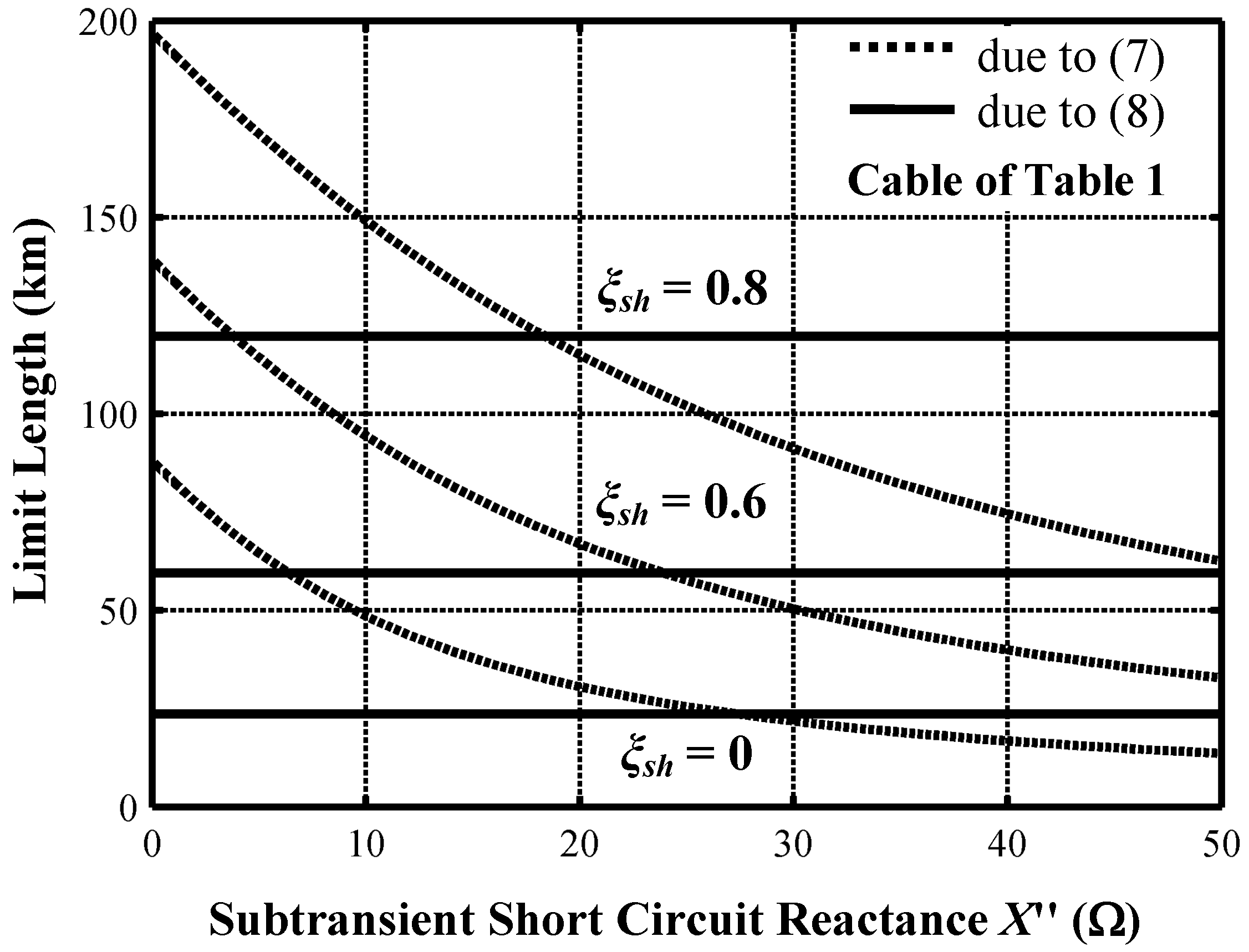
The curves of Figure 4 and Figure 5 are computed for the cable of Table 1: both show that the constraint (8) is almost always decisive for the determination of ξ_sh, unless there is an agreement with the manufacturer for a circuit breaker with higher I_NL.

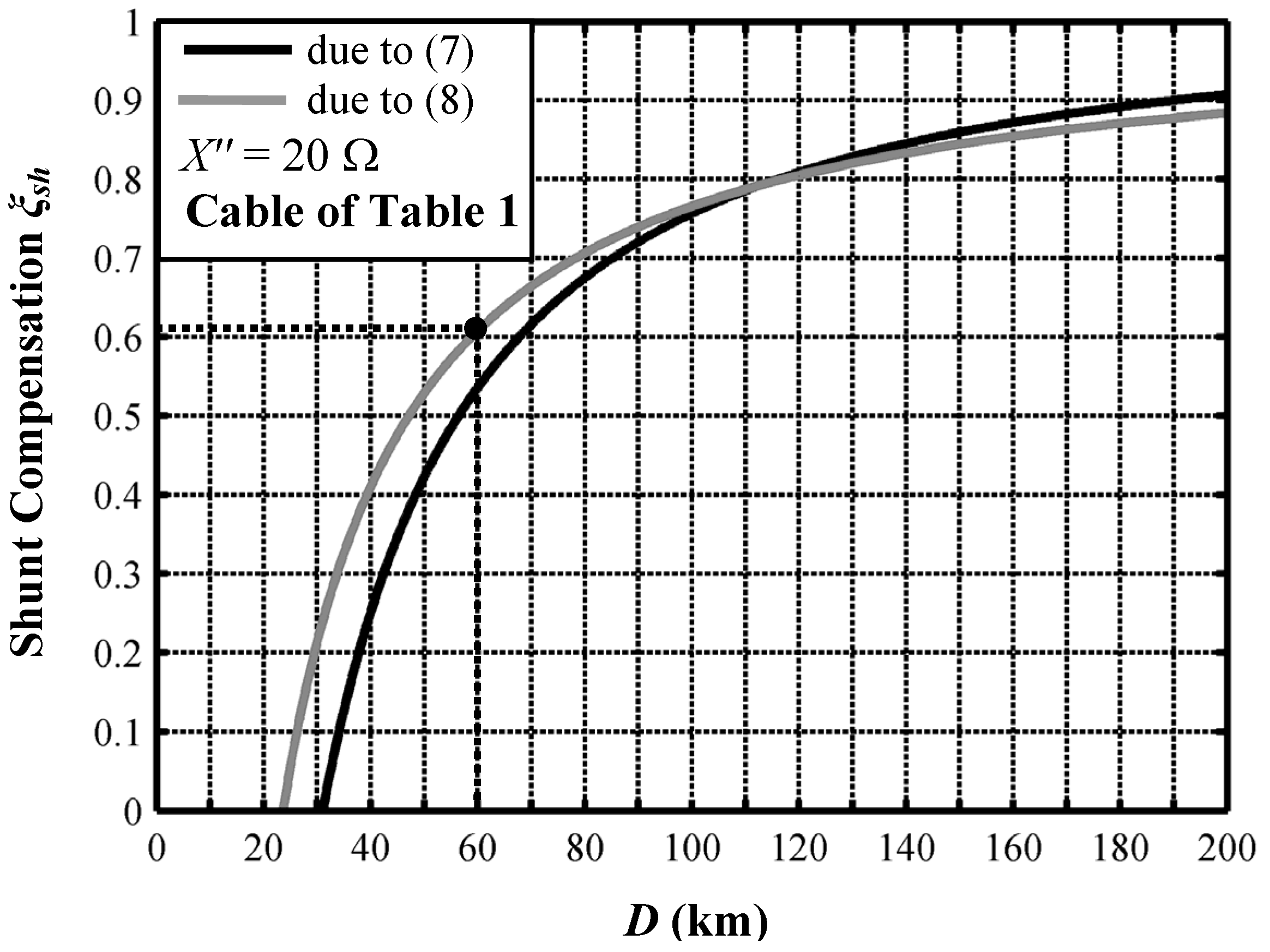
Figure 5 clearly defines the values of shunt reactive compensation degree ξ_sh which fulfills the relations (7) or (8): it shows which is the more limiting criterion as a function of the line length. It appears almost trivial to note that the considerations regarding the additional constraint of (7) must be performed also for the energization by the port R, by introducing for the parameters U_o and X^" suitable values in consideration of the supply grid linked to R: the detection and the choice of the “best end switching” [5] are mentioned by CEGB as effective experienced practices in network operations. Moreover, the cases where the steady state capacitive power absorbed by the cables (Q_NL = 3U_o I_NL) exceeds the ability of synchronous generators (dangerous self-excitation conditions), located in close proximity of the cable installation, must be avoided. In any case, it is advisable that the TSO, when planning a new link, performs both detailed power flows and network simulations.

Figure 4. Limit lengths due to the constraints (7) and (8) for cable of Table 1.

Figure 4. Limit lengths due to the constraints (7) and (8) for cable of Table 1.

Figure 5. Reactive compensation degree as a function of cable length due to the constraints (7) and (8) for cable of Table 1 and X'' = 20 Ω.

Figure 5. Reactive compensation degree as a function of cable length due to the constraints (7) and (8) for cable of Table 1 and X'' = 20 Ω.

Table 1. EHV AC Cable under study.

Cable cross-sectional area	mm2	2500 Cu
Conductor diameter (Milliken type with six sectors)	mm	63.4
XLPE insulation diameter	mm	119.9
Metallic screen diameter	mm	130.1 Al
Screen cross-sectional area	mm2	$\cong$ 500
PE jacket diameter	mm	141.7
Total mass	kg/m	37

Table 1. EHV AC Cable under study.

Cable cross-sectional area	mm2	2500 Cu
Conductor diameter (Milliken type with six sectors)	mm	63.4
XLPE insulation diameter	mm	119.9
Metallic screen diameter	mm	130.1 Al
Screen cross-sectional area	mm2	$\cong$ 500
PE jacket diameter	mm	141.7
Total mass	kg/m	37

3. Insertion of Shunt Reactors in the MCA

Once the model of CB UGC is completed in the MCA [1 ÷ 3], it is necessary to consider the presence of lumped shunt reactive compensation.

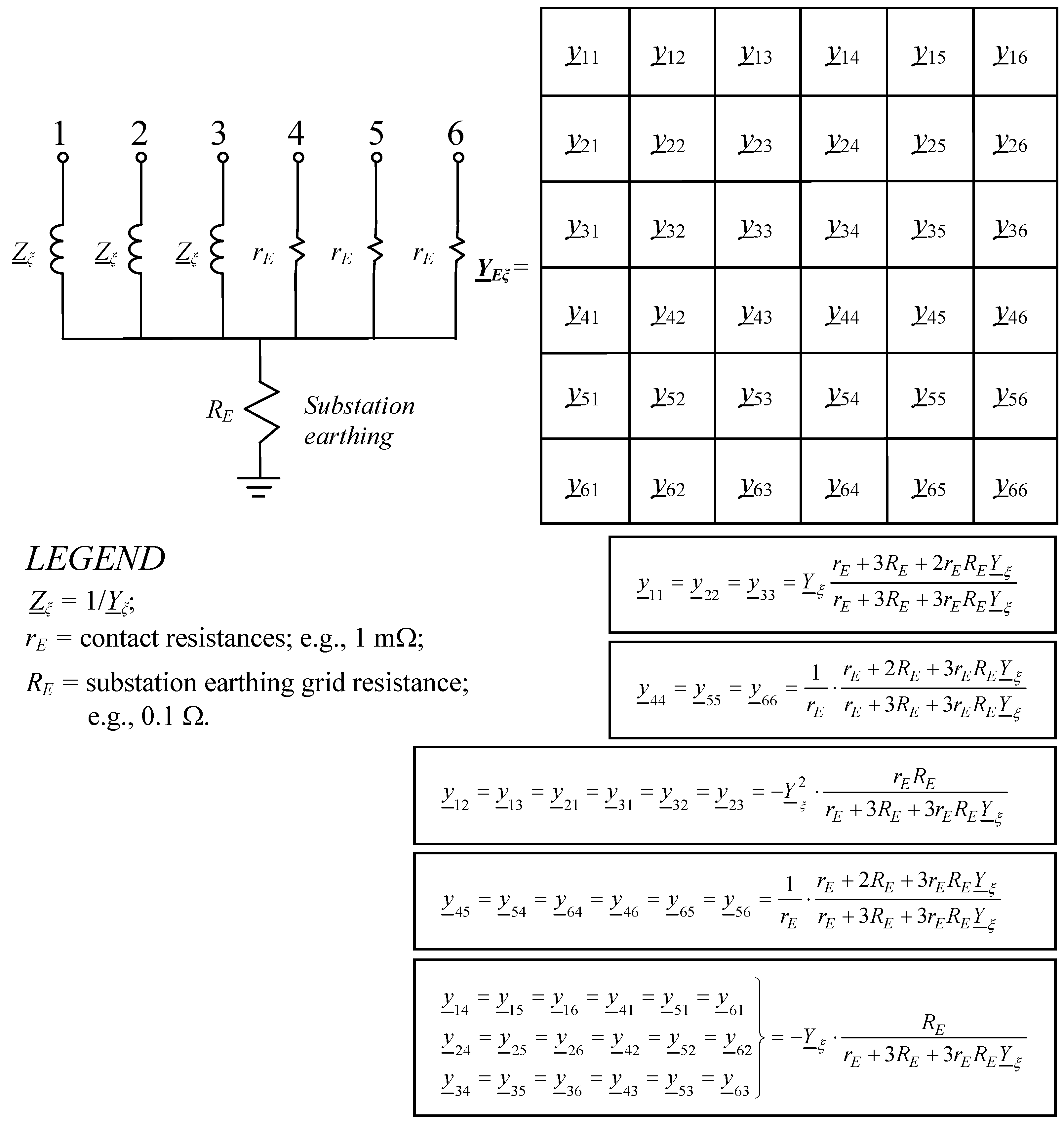
Figure 6. Admittance matrix Y_Eξ for shunt reactors and screen earthing.

Figure 6. Admittance matrix Y_Eξ for shunt reactors and screen earthing.

The insertion between phases 1, 2, 3 and the earth of three single-phase reactors (or three-phase ones with unchained magnetic flux) can be easily accounted for by means of the admittance matrix Y_Eξ to be overlapped in the right locations. There are two methods to compute the admittance matrix Y_Eξ; the former is a direct calculation by the inspection method as in Figure 6. The latter is computing firstly the matrix Z_Eξ (6 × 6), as shown in (9), where Z_ξ = 1/Y_ξ. Successively by matrix inversion, it is possible to obtain the admittance matrix Y_Eξ = (Z_Eξ)⁻¹. The computation of the shunt susceptance Y_ξ has been already presented in Section 2.

Once the matrix Y_Eξ has been computed, it must be overlapped in the suitable positions (i.e., only at the two ends or also at intermediate locations) on the general admittance matrix which accounts for the cable [1,2,3].

(9)

4. Case Study

The abovementioned theory is applied to a directly buried (see Figure 7, Table 1 and Table 2) shunt compensated long UGC (d = 60 km) (as highlighted with a dot in Figure 5, for d = 60 km it yields ξ_sh = 0.608). The UGC is cross-bonded (CB) with phase transpositions (PTs).

Table 2. Data assumed in MCA.

Multiconductor cell length		km	0.125
Cable drum (Minor section)		km	0.625
Cross-bonding section Length (Major section)		km	1.875
Substation earthing	RE	Ω	0.1
Earth resistivity	ρsoil	Ω m	100
Cross-bonded box resistance	R	Ω	10
Screen resistance at 78.2 °C (50 Hz)	rsh	mΩ/km	70.0
Link resistance	rE	mΩ	1
Shunt compensation degree	ξsh		0.608
Number of shunt compensation stations			4 (or 2)
Ampacity		A	1788
Load at receiving-end		MW + jMvar	1214 + j0

Table 2. Data assumed in MCA.

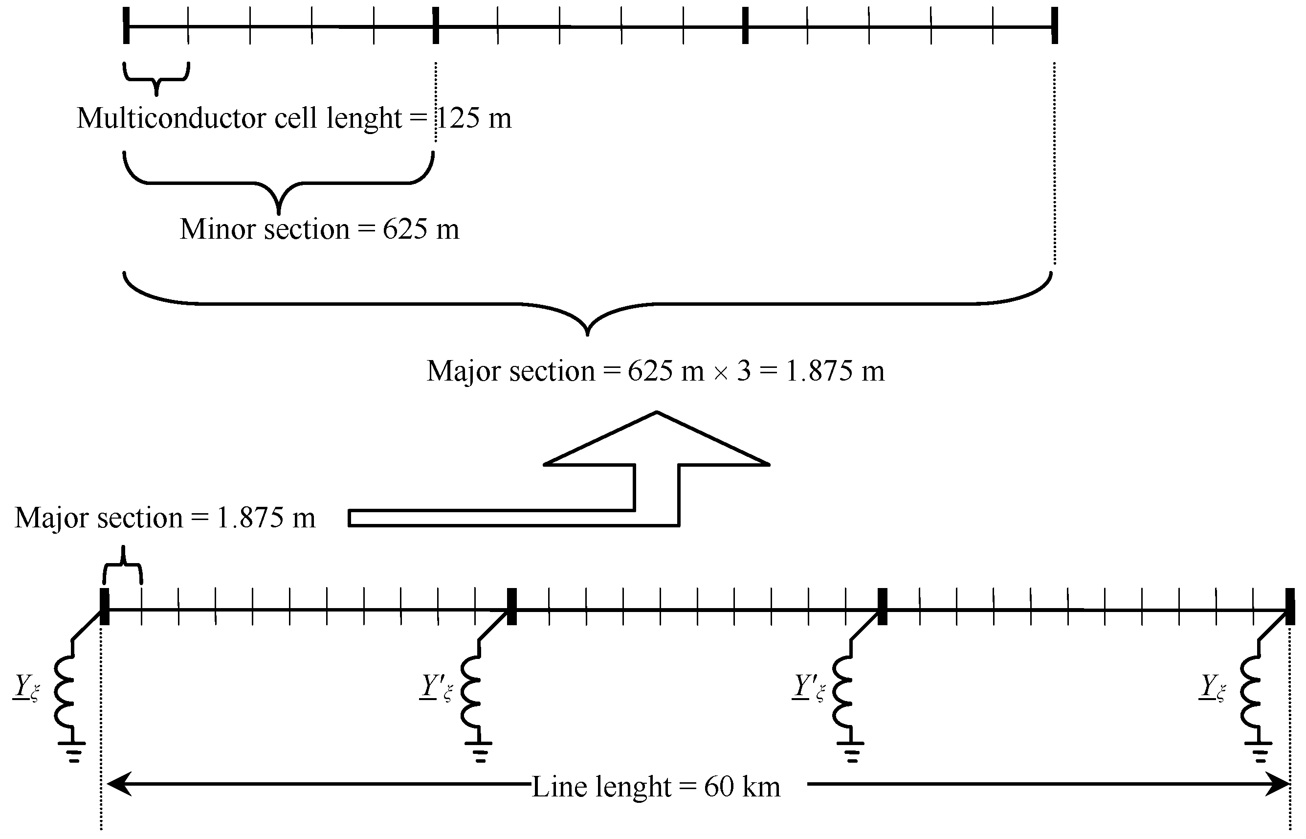
Multiconductor cell length		km	0.125
Cable drum (Minor section)		km	0.625
Cross-bonding section Length (Major section)		km	1.875
Substation earthing	RE	Ω	0.1
Earth resistivity	ρsoil	Ω m	100
Cross-bonded box resistance	R	Ω	10
Screen resistance at 78.2 °C (50 Hz)	rsh	mΩ/km	70.0
Link resistance	rE	mΩ	1
Shunt compensation degree	ξsh		0.608
Number of shunt compensation stations			4 (or 2)
Ampacity		A	1788
Load at receiving-end		MW + jMvar	1214 + j0

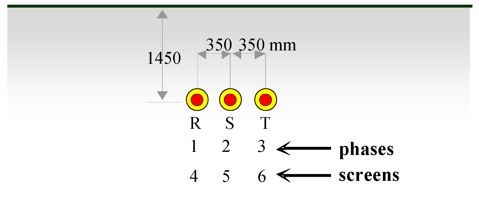
Figure 7. Single-circuit CB UGC.

Figure 7. Single-circuit CB UGC.

The whole multiconductor system is shown in Figure 8, which helps visualizing both the cable subdivision in elementary cells (with indication of minor and major sections) and the lumped shunt compensation locations. In this case, the minor sections have all equal lengths but this method also suits very well the case of different lengths (as in the real installations).

Figure 8. Subdivision of the CB single-circuit cable line with indication of lumped shunt compensation locations.

Figure 8. Subdivision of the CB single-circuit cable line with indication of lumped shunt compensation locations.

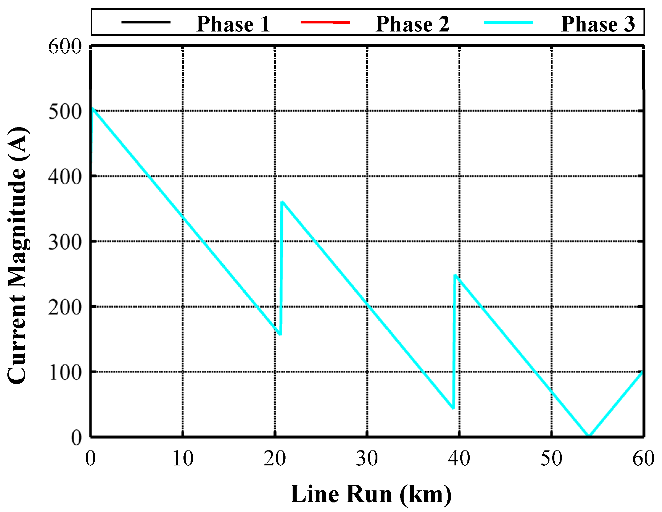
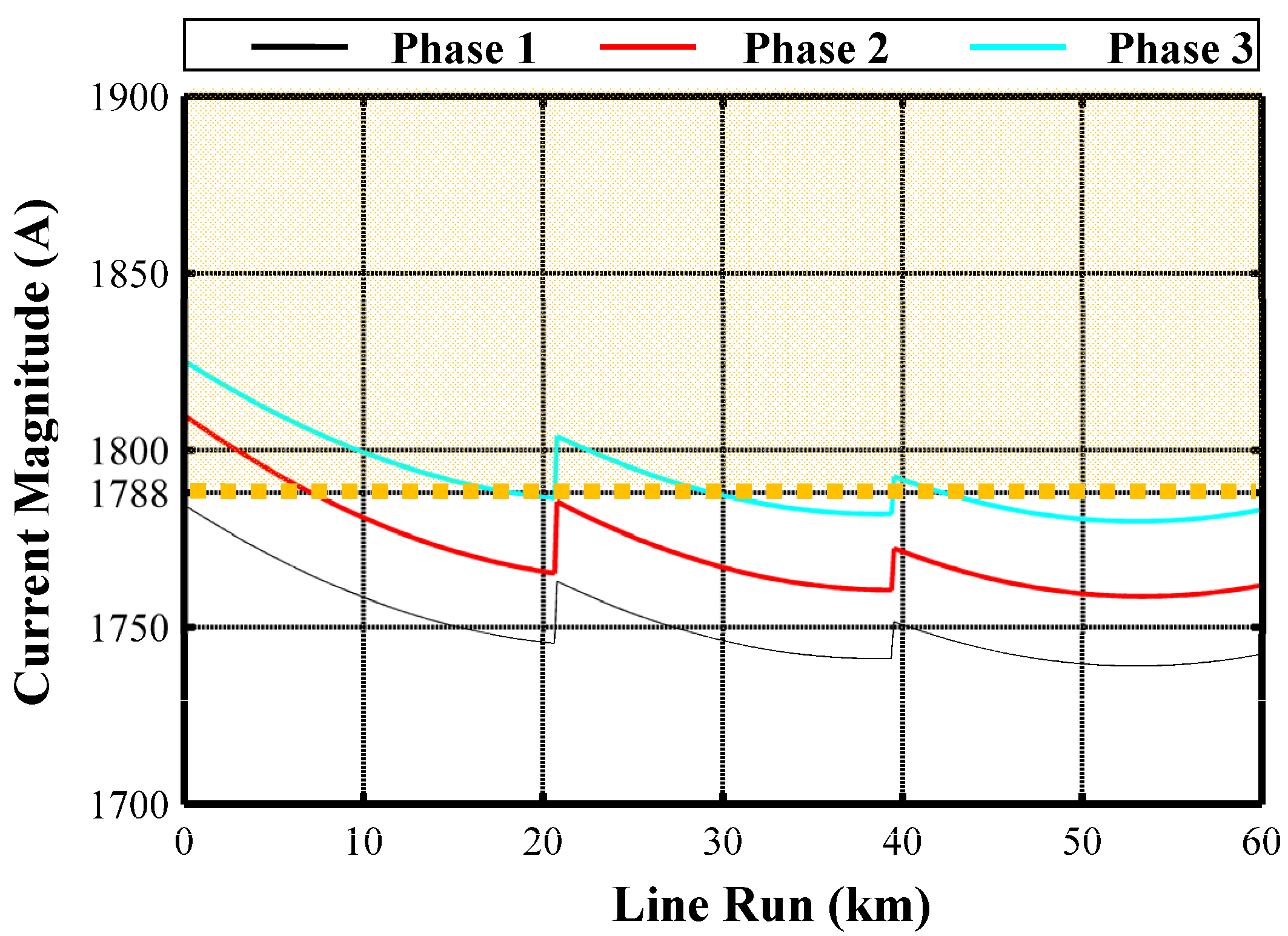
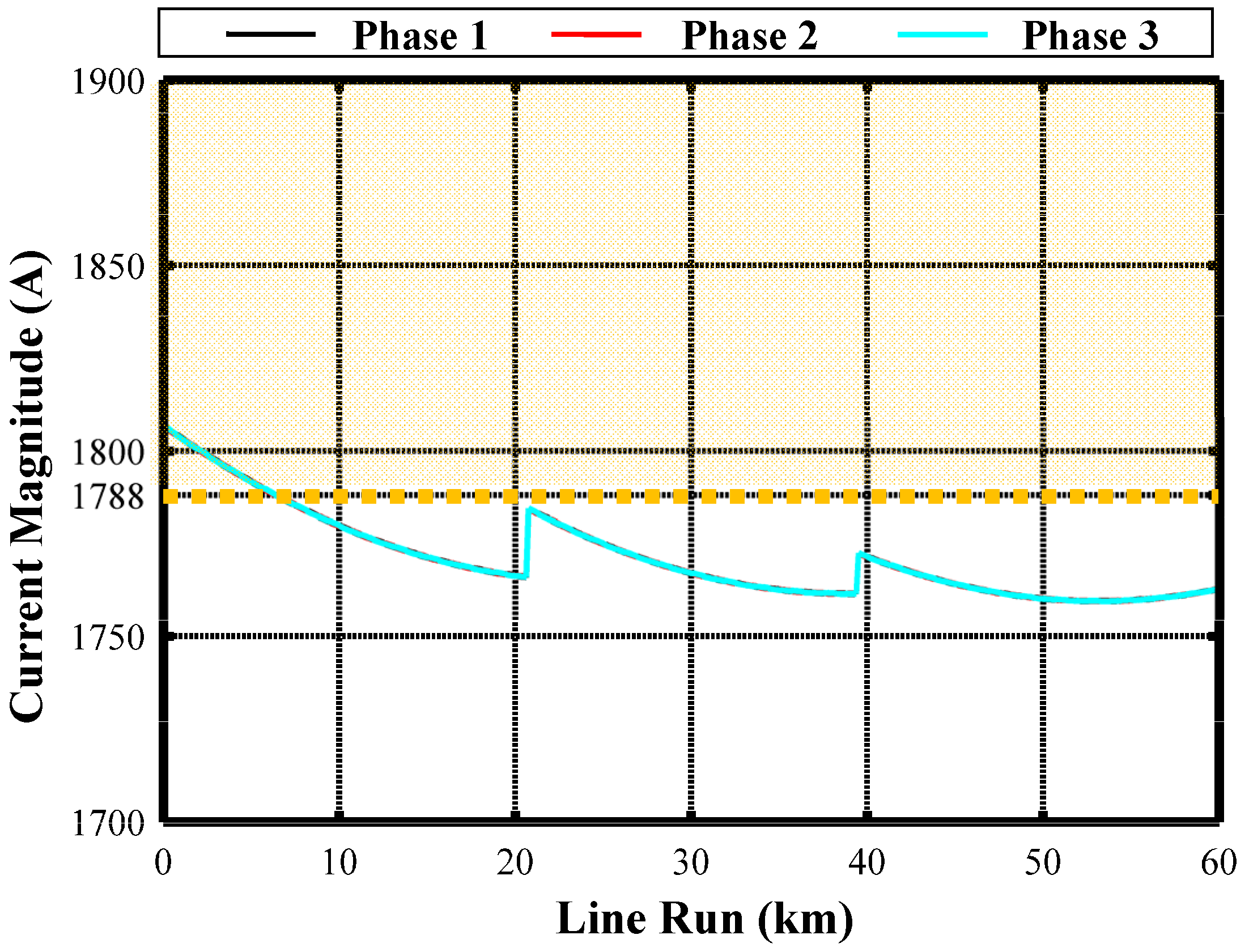
Figure 9 shows the phase current magnitudes along the cable: they are in whole accordance with those obtained by means of the single-circuit positive sequence analysis [3]. Obviously, the multiconductor analysis gives a higher accuracy of the system knowledge. Figure 9 shows a light exceeding of the ampacity (grey zone) in the first kilometres, but it is not problematic when consideration is given to the natural fluctuations of the line operation.

Figure 9. Phase current magnitudes along the compensated single-circuit cable, in CB with PTs.

Figure 9. Phase current magnitudes along the compensated single-circuit cable, in CB with PTs.

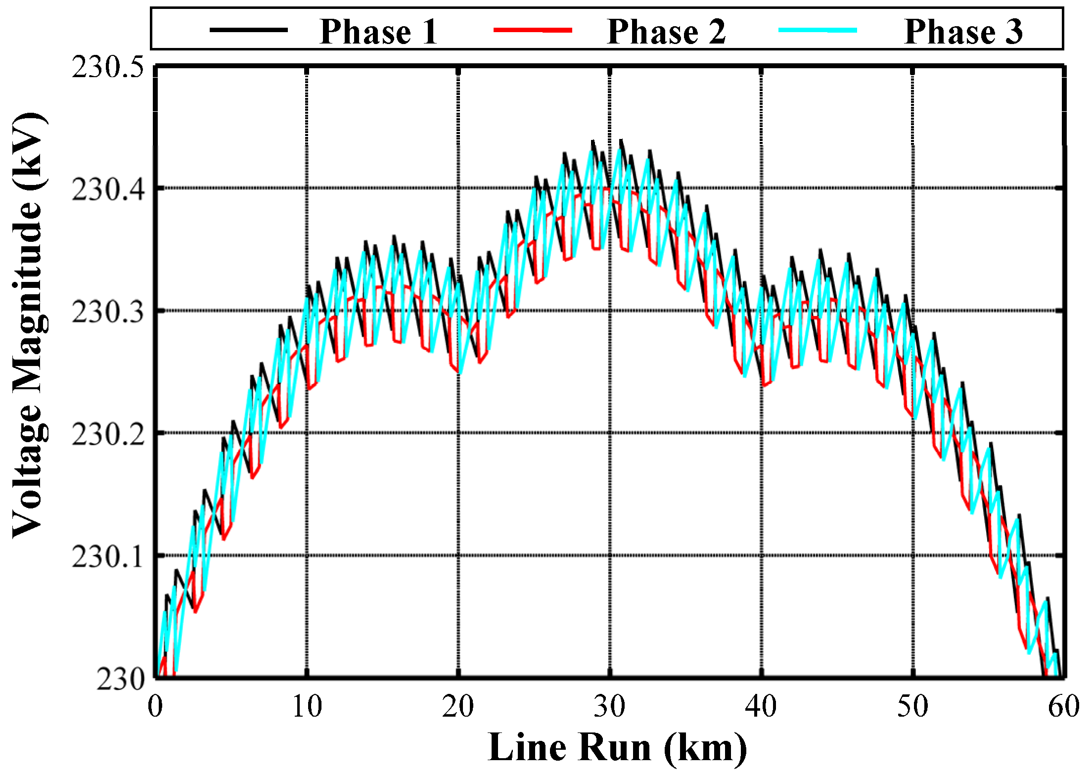
Figure 10 shows the phase voltage magnitudes which are in whole accordance with those obtained by means of single-circuit positive sequence analysis: nevertheless, Figure 10 shows the great accuracy and detail of MCA and a negligible voltage asymmetry.

Figure 10. Phase voltage magnitudes along the compensated single-circuit cable in CB with PTs.

Figure 10. Phase voltage magnitudes along the compensated single-circuit cable in CB with PTs.

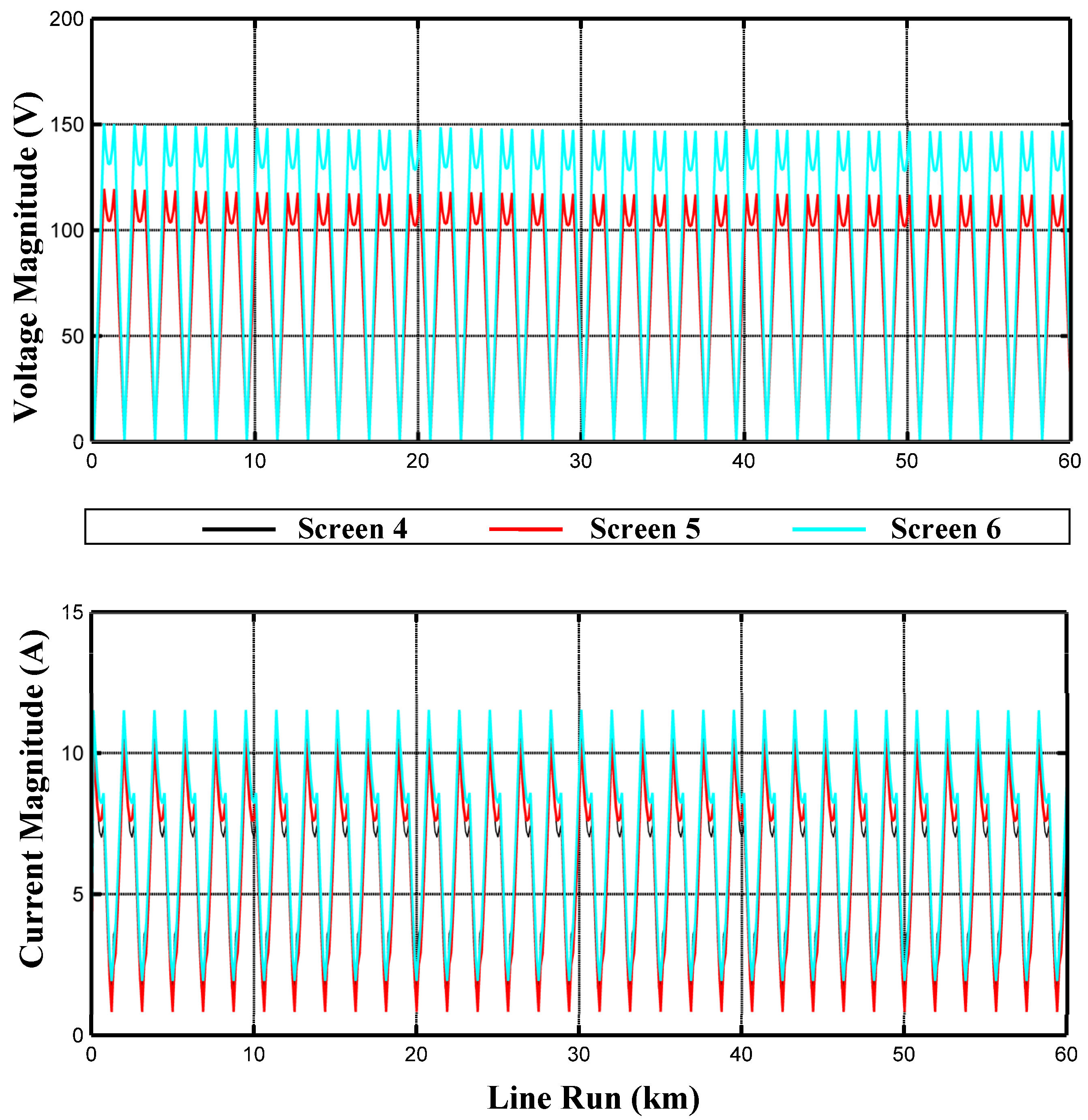
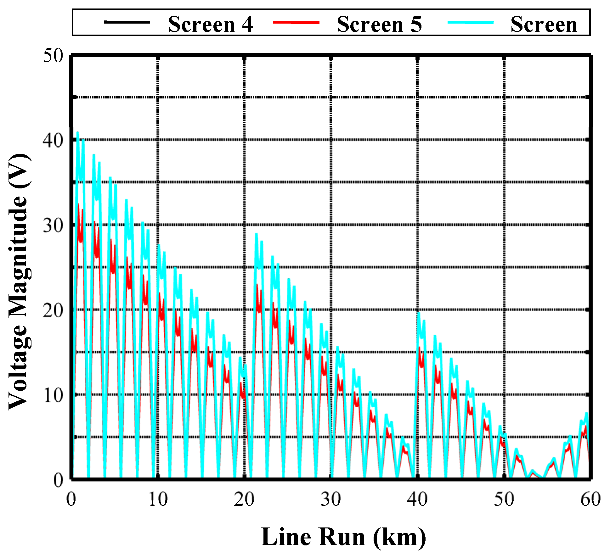
One of the great possibilities offered by the multiconductor analysis is the knowledge of the screen electric behaviours. Figure 11 shows the screen voltage and current magnitudes along the cable.

Figure 11. Screen voltage and current magnitudes along the compensated single-circuit cable in CB with PTs.

Figure 11. Screen voltage and current magnitudes along the compensated single-circuit cable in CB with PTs.

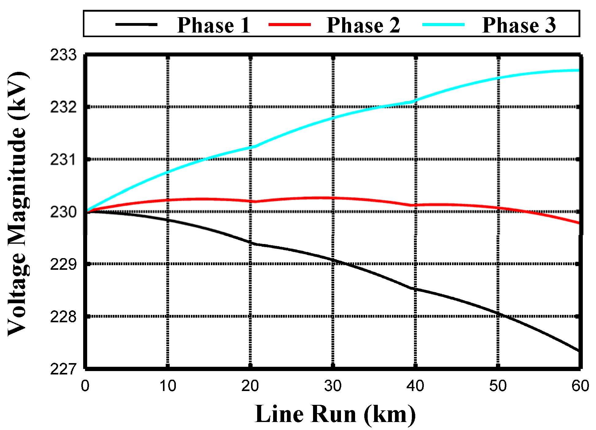
The screen currents of induced nature are extremely low so demonstrating the effectiveness of CB arrangement: the residue currents are those of capacitive nature. The no-load steady-state regime has also been investigated: Figure 12 shows the phase current magnitudes along UGC. Since the use of PTs, the behaviours of the three phases are very similar to those derived by means of single-phase positive sequence circuit: therefore, they are visible as a unique curve. Moreover in Figure 13 the screen voltage magnitudes are shown: the induced voltages in the screens are strictly depended upon the inducing phase currents.

Figure 12. Phase current magnitudes along the compensated UGC in CB with PTs at no-load.

Figure 12. Phase current magnitudes along the compensated UGC in CB with PTs at no-load.

Figure 13. Screen voltage magnitudes along the compensated single-circuit cable in CB with PTs at no-load.

Figure 13. Screen voltage magnitudes along the compensated single-circuit cable in CB with PTs at no-load.

All the abovementioned situations can be studied also with a single-phase positive sequence model even if the MCA allows a deeper knowledge of the power system. In the following more asymmetrical situations are shown. In fact, as well-known, the CB performed without PTs (many TSOs do not perform phase transpositions) has a higher level of asymmetry so that, in these cases, the MCA becomes an unavoidable tool for engineering investigations.

In order to demonstrate this assertion, Figure 14 and Figure 15 (which must be compared with Figure 9 and Figure 10) are shown.

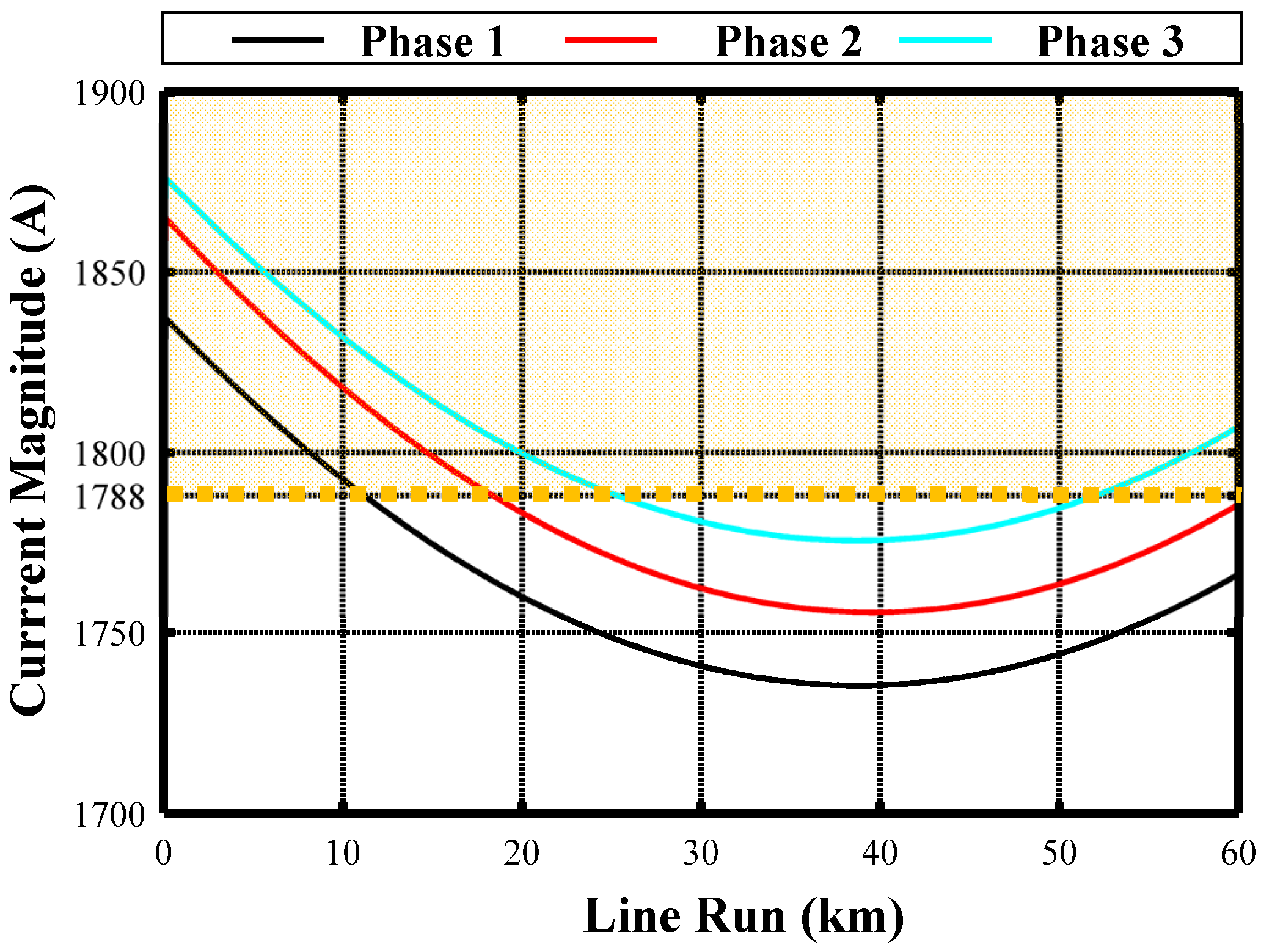
Figure 14. Phase current magnitudes along the compensated single-circuit cable in CB without PTs.

Figure 14. Phase current magnitudes along the compensated single-circuit cable in CB without PTs.

Figure 15. Phase voltage magnitudes along the compensated single-circuit cable in CB without PTs.

Figure 15. Phase voltage magnitudes along the compensated single-circuit cable in CB without PTs.

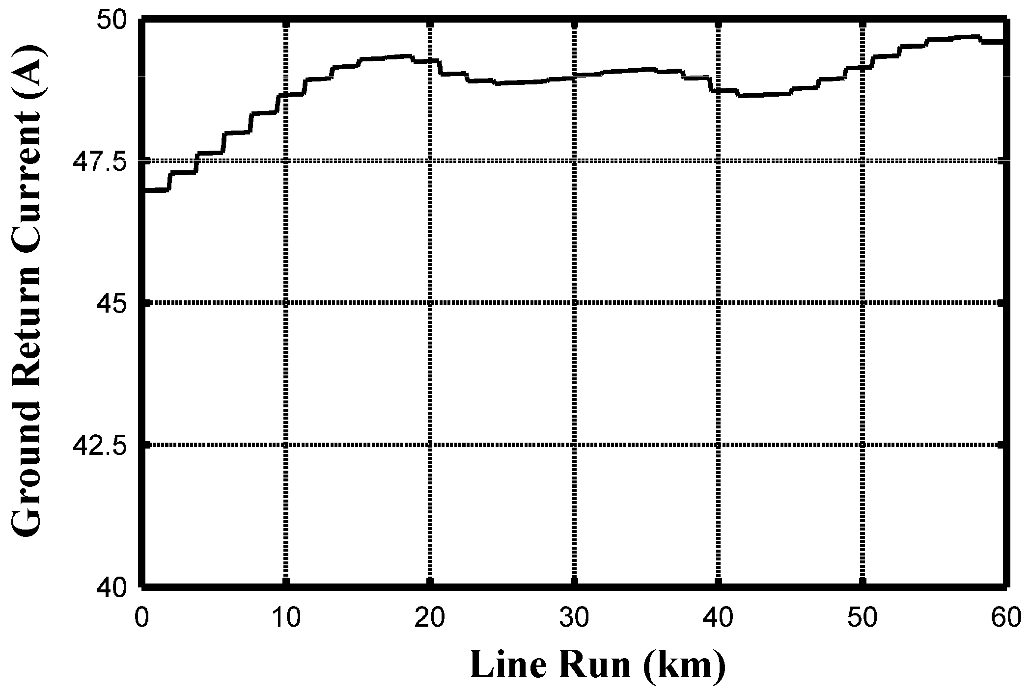
They represent phase current and voltage magnitudes, respectively, for CB performed without PTs. The behaviours of the three phases 1, 2, 3 are rather different and in the case of Figure 14 the ampacity limit is exceeded by both phase 2 and 3. Another important feature of CB without PTs is the fact that it implies a ground return current, as Figure 16 shows. It is worth noting that this current is always present in steady-state operation so that possible electromagnetic interferences could arise with nearby parallel metallic systems. The shunt compensation only at the two ends is possible but it gives wider stretches of ampacity exceeding as Figure 17 clearly shows. In this case, the ampacity is exceeded (grey zone) by all the three phases and for a long stretch of UGC length. Moreover, power losses (average value equal to 135 kW/km) are higher than those due to the shunt compensation also at intermediate locations (average value equal to 133 kW/km).

Figure 16. Ground return current magnitude for CB UGC without PTs.

Figure 16. Ground return current magnitude for CB UGC without PTs.

Figure 17. Phase current magnitudes along the compensated single-circuit cable in CB without PTs and compensated only at the two ends (as in Figure 1).

Figure 17. Phase current magnitudes along the compensated single-circuit cable in CB without PTs and compensated only at the two ends (as in Figure 1).

5. Conclusions

The power of the self-made MCA is the applicability to very different systems, e.g., HVDC armoured cables [6], gas insulated lines [7,8,9], overhead lines with one or more earth-wires [10,11] and ac high speed railways [12]. In this paper, the MCA has been applied to a single-core CB UGC with shunt compensation. The single-phase positive sequence analysis can be sufficient for engineering purposes, but the paper has demonstrated that there are some cases (i.e., CB without phase transpositions) where only the MCA provides a full understanding of the power system. Moreover, the paper has shown that the shunt compensation only at the two ends is also possible for long UGC, but the use of intermediate shunt compensation stations gives both lower power losses and less wide stretches of exceeded ampacity.