Effects of a Green Space Layout on the Outdoor Thermal Environment at the Neighborhood Level

Abstract

This study attempted to address the existing urban design needs and computer-aided thermal engineering and explore the optimal green space layout to obtain an acceptable thermal environment at the neighborhood scale through a series of building energy and computational fluid dynamics (CFD) simulations. The building-energy analysis software eQUEST and weather database TMY2 were adopted to analyze the electric energy consumed by air conditioners and the analysis results were incorporated to derive the heat dissipated from air conditioners. Then, the PHOENICS CFD software was used to analyze how the green space layout influences outdoor thermal environment based on the heat dissipated from air conditioners and the solar heat reemitted from the built surfaces. The results show that a green space located in the center of this investigated area and at the far side of the downstream of a summer monsoon is the recommended layout. The layouts, with green space in the center, can decrease the highest temperature by 0.36 °C.

1. Introduction

In recent years, the amount of people immigrating to urban area keeps on increasing and urbanization has become the trend in developed or developing countries. Due to the growing population demands, the presence of more buildings and more people begins to transform the landscape and such an activity will have an impact on the urban environment [1]. The so called urban heat island effect causes rising temperatures in an urban area. Takahashi et al. [2] argue that the causes for the rising temperature in an urban area are: decreasing green space, low wind velocity caused by dense building, and pavement materials. For the research of urban heat island effect, many adopt computational fluid dynamics (CFD) to analyze the distribution of buildings and environmental factors in different types of urban area, and to then study the changes of temperature and wind field [3,4]. Urban heat islands are considered to be a cumulative consequence of all the above mentioned impacts. Oke [5] offers a concise description of atmospheric layers that is highly related to heat island research in a variety of disciplines.

Urban heat islands are formed by the temperature rise in any human-made area in comparison to the lower temperature levels of the nearby natural landscape of the area. If city block configurations are in coordination with the arrangement of the infrastructure (urban design elements: blue and green belts), the degree of the urban heat island effect and the microenvironment around the block will be influenced. Jeong and Yoon [6] investigated green building cases to quantify the outdoor thermal comfort and heat island potential change throughout a day according to several design variables (building type, site planning type, façade direction, and landscape ratio). Chen et al. [7] performed coupled simulations of convection, radiation and conduction to evaluate the outdoor thermal environment over different urban blocks, including a high-rise area and a mid-rise area in Tokyo, Japan, to compare the effects of measures such as the heat release point and means of air-conditioning, greening, high surface albedo, and traffic volume. Synnefa et al. [8] used CFD simulation for evaluating the thermal and energy impact of applying different samples of materials on outdoor spaces (roads). The results show that surface and air temperatures are decreased colored thin layer samples are applied.

The objective of the present study was to provide insights into urban design alternatives that will improve the considered above-mentioned thermal environment, for which little or no information is available. In so doing, the eQUEST software was used to estimate the heat dissipated from air conditioners, and then a CFD simulation was adopted to examine how city block configurations influence the outdoor thermal environment at the neighborhood scale to explore the possibility of reducing the heat effect.

2. From the Energy Consumption of Buildings to the Urban Heat Island Effect

2.1. Study Objective

Computer-based simulation is accepted by many studies as a tool for evaluating a building’s energy. There are many different types of computer-based simulation tools that are available for performing whole-building simulations. For example, the DOE2 software application is an expert system supporting energy auditing. The QUick Energy Simulation Tool (eQUEST), a quick energy simulation tool developed by Doe2.com, is a sophisticated, yet easy to use, freeware building energy use analysis tool that provides professional-level results with an affordable level of effort (eQUEST is available from the U.S. Department of Energy, please see http://www.doe2.com [9] for documentation).

In this study, eQUEST Version 3.63 was adopted as an analysis tool, and a residence in an urban area was chosen as the object of study. Simulations were performed, and then, in accordance with the effectiveness factors of an air conditioner, the air conditioner energy consumption was converted to a heat emission source and became one of the heat sources of the outdoor environment.

The simulated area (as shown in Figure 1a) is the Zhengzeliao consolidation zone in Tainan City because it is a newly planned and densely populated residential area, most of the families are small and there are neighborhood parks (green space plus simple facilities) in accordance with the urban plan. City blocks in the Zhengzeliao consolidation zone (as shown in Figure 1b) were modified into rectangles and rearranged with green spaces (assuming that the area of a green space equals one city block) to form a nine-box (3 × 3) configuration. The size of a city block composed of reinforced concrete (RC) buildings is 80 × 22 m (as shown in Figure 1c), and the width of the asphalt road is 13 m. A west-facing building in the city block was taken as the simulation object (the area defined by black dotted lines in Figure 1c), because it shows the worst solar heat gain conditions. In the building, there is a living room, a kitchen, a bedroom, a bathroom, a balcony and a public space. The floor plan of the building is shown in Figure 2. The weather database TMY2, based on the data system of the Central Meteorology Bureau of Taiwan, was used in the simulation work.

Figure 1. Object of research: (a) The area of this research (yellow dotted lines); (b) Modified area of research; (c) A city block composed by buildings.

Figure 1. Object of research: (a) The area of this research (yellow dotted lines); (b) Modified area of research; (c) A city block composed by buildings.

Figure 2. Floor plans of the main simulation target (not to scale): (a) 1st floor; (b) 2nd floor; (c) 3rd floor; (d) 4th floor.

Figure 2. Floor plans of the main simulation target (not to scale): (a) 1st floor; (b) 2nd floor; (c) 3rd floor; (d) 4th floor.

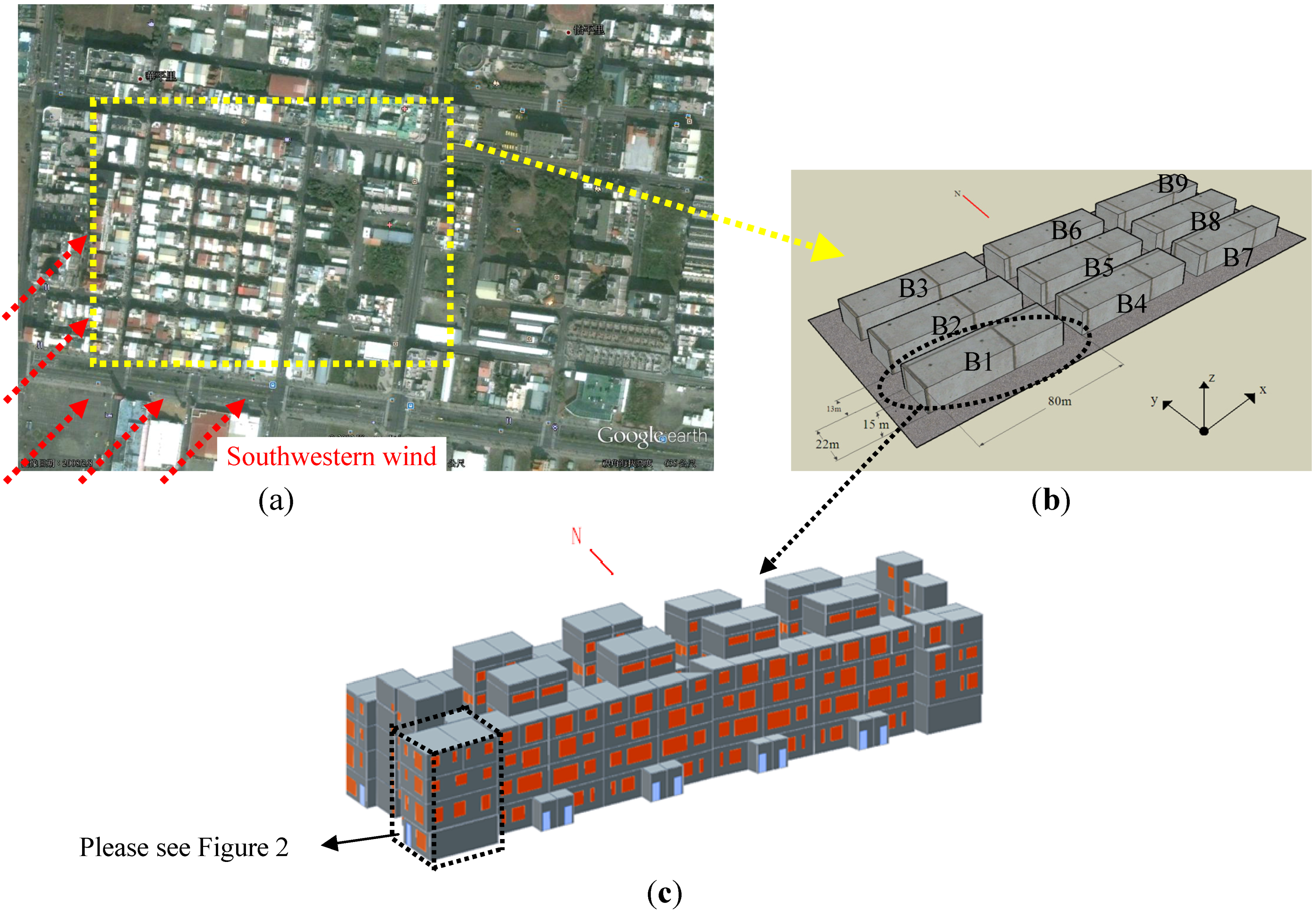
2.2. Building Materials and Conditions of Space Use

2.2.1. Structure Materials

Most Taiwanese residences are RC structures. Although steel structures are increasingly used, they are mostly used to build tall buildings, therefore, the structural material used in this study is RC. In terms of window glass, it is assumed to be a clear glass with a thermal transmittance (U-value) of 5.67 W/(m² K), a shading coefficient (SC) of 0.88, and a visible light transmittance (VT) of 0.86. Table 1 and Table 2 show the detailed illustrations and thermal properties of the roof and the external wall.

Table 1. Details of the RC roof and the thermal properties of each layer of material.

Illustration	Detailed construction	Thermal conductivity [W/(m K)]	Thickness [cm]	U-value [W/(m² K)]
	Outdoor convection	23	-	1.141
	Insulation bricks	1.5	3.5
	Styrofoam	0.040	2
	PU layer	0.05	0.2
	Cement mortar	1.5	1.5
	RC	1.4	15
	Cement mortar	1.5	1.5
	Indoor convection	7	-

Table 1. Details of the RC roof and the thermal properties of each layer of material.

Illustration	Detailed construction	Thermal conductivity [W/(m K)]	Thickness [cm]	U-value [W/(m² K)]
	Outdoor convection	23	-	1.141
	Insulation bricks	1.5	3.5
	Styrofoam	0.040	2
	PU layer	0.05	0.2
	Cement mortar	1.5	1.5
	RC	1.4	15
	Cement mortar	1.5	1.5
	Indoor convection	7	-

Table 2. Details of the RC exterior wall and the thermal properties of each layer of material.

Illustration	Detailed construction	Thermal conductivity [W/(m K)]	Thickness [cm]	U-value [W/(m² K)]
	Outdoor convection	23	-	3.497
	Ceramic tile	1.3	1
	Cement mortar	1.5	1.5
	RC	1.4	15
	Cement mortar	1.5	1
	Indoor convection	9	-

Table 2. Details of the RC exterior wall and the thermal properties of each layer of material.

Illustration	Detailed construction	Thermal conductivity [W/(m K)]	Thickness [cm]	U-value [W/(m² K)]
	Outdoor convection	23	-	3.497
	Ceramic tile	1.3	1
	Cement mortar	1.5	1.5
	RC	1.4	15
	Cement mortar	1.5	1
	Indoor convection	9	-

2.2.2. Residence Members

In accordance with statistics from the Directorate-General of Budget, Accounting and Statistics, Executive Yuan, the average number of members in each residence in Taiwan is between 3.47 and 3.61. It was assumed that there are four members in each residence, including parents and two school-aged children.

2.2.3. Basic Electrical Appliances

Due to different living conditions and needs, it is difficult to list all of the electrical appliances in each residence. Thus, in the simulation, only the most necessary and frequently used appliances were taken into consideration (as shown in Table 3).

Table 3. Electricity consumption of household appliances.

Space	Power consumed [W]	Illumination density [W/m²]
Living room	Television: 130	8.07
Kitchen	Cooker: 600, range hood: 350, microwave oven: 1200, refrigerator: 130, electric pot: 750, dishwasher: 200	6
Master bedroom	Television: 130	6.5
Bedroom	Computer: 120	6
Bathroom	Hair dryer: 800	6.5
Balcony	Washing machine: 420	5
Public space	None	6

Table 3. Electricity consumption of household appliances.

Space	Power consumed [W]	Illumination density [W/m²]
Living room	Television: 130	8.07
Kitchen	Cooker: 600, range hood: 350, microwave oven: 1200, refrigerator: 130, electric pot: 750, dishwasher: 200	6
Master bedroom	Television: 130	6.5
Bedroom	Computer: 120	6
Bathroom	Hair dryer: 800	6.5
Balcony	Washing machine: 420	5
Public space	None	6

2.2.4. Occupation Period of Major Spaces

The typical daily occupation periods of major spaces in the target building are shown in Table 4.

Table 4. Daily occupation period of major spaces (00:00 to 23:00).

Interior spaces	Time
In workdays	0	1	2	3	4	5	6	7	8	9	10	11	12	13	14	15	16	17	18	19	20	21	22	23
Living room/kitchen
Main bedroom
Bedroom
On weekend	0	1	2	3	4	5	6	7	8	9	10	11	12	13	14	15	16	17	18	19	20	21	22	23
Living room/kitchen
Main bedroom
Bedroom

Table 4. Daily occupation period of major spaces (00:00 to 23:00).

Interior spaces	Time
In workdays	0	1	2	3	4	5	6	7	8	9	10	11	12	13	14	15	16	17	18	19	20	21	22	23
Living room/kitchen
Main bedroom
Bedroom
On weekend	0	1	2	3	4	5	6	7	8	9	10	11	12	13	14	15	16	17	18	19	20	21	22	23
Living room/kitchen
Main bedroom
Bedroom

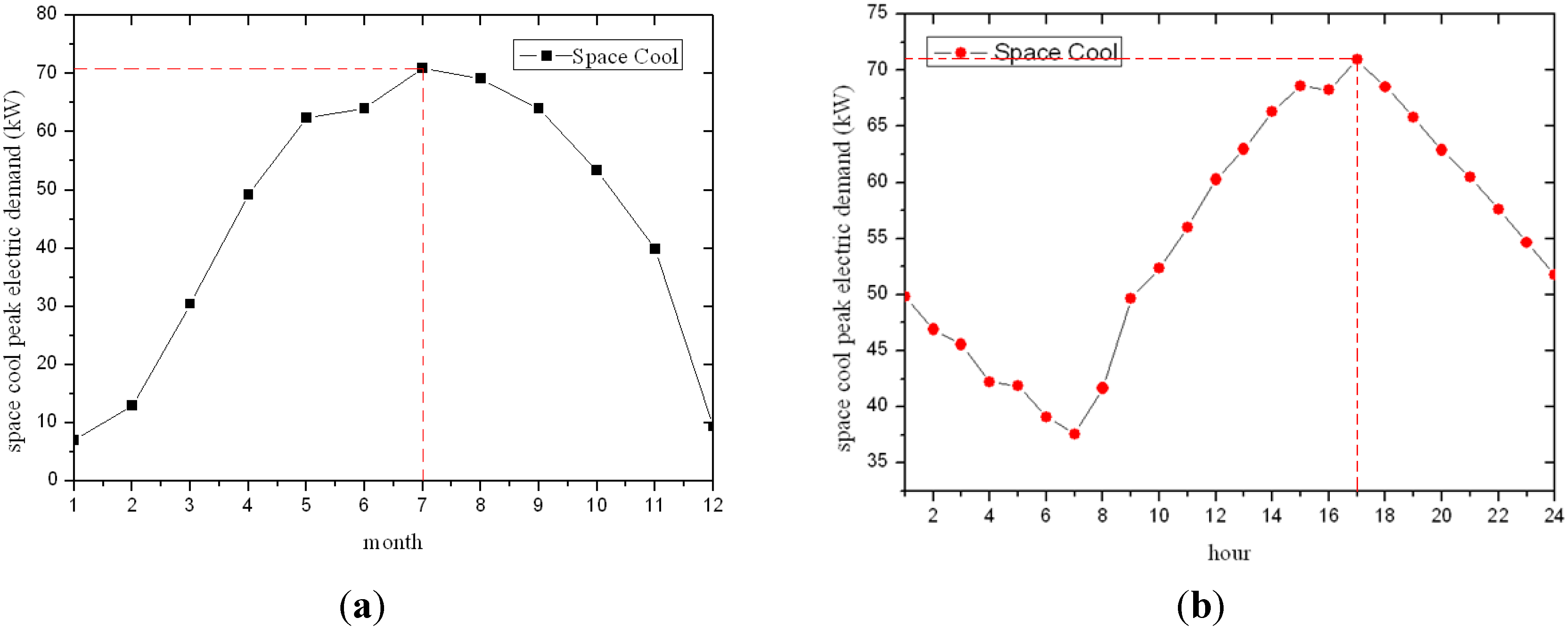
2.2.5. Air Conditioner Capacities and Their Operating Periods

Air conditioners come in various types. In general, they can be classified as a window-type, a packaged-type, a separate-type or centralized systems. For the buildings in Taiwan’s urban areas, separate-type air conditioners have the advantages of reducing indoor noise and having a high mobility for installation. This type of air conditioner includes an indoor unit and an outdoor unit, or one outdoor unit combined with multiple indoor units, and it is the most common type of air conditioner selected by families. The cooling capacity is approximately 2000–10,000 kcal/h. The type of air conditioner applied in this study was the one-to-one separate type, and the operating periods were based on the assumed time sections in Table 4. The system automatically activated when the temperature was higher than 28 °C within the indicated time periods; the room temperature was maintained at 26 °C once activated. The Energy Efficiency Ratio (EER) value of the air conditioners was set at 3.45 (W/W) for the simulation according to the latest regulations of the Bureau of Energy, Taiwan, in 2011. The lowest EER value for separate-type air conditioners was less than 4.0 kW.

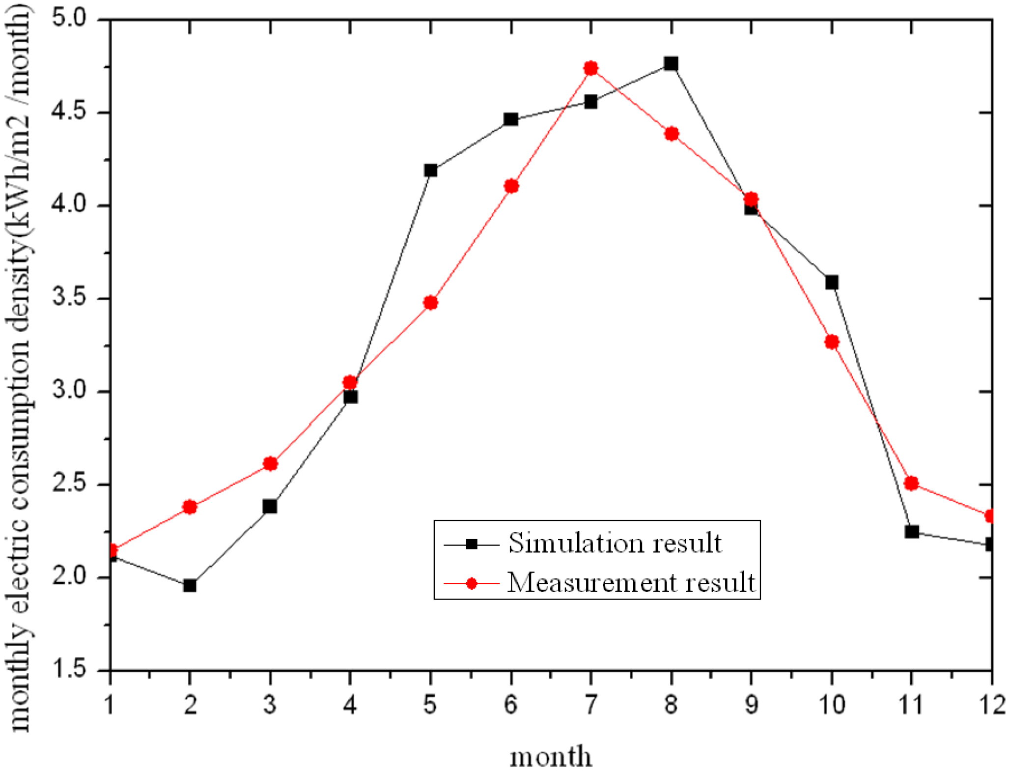
2.3. Comparison of Energy Consumption between Simulation and Measured Results

The study compared the simulation results of residential buildings with the largest energy consumption (facing west) to the measured values [10,11], as shown in Figure 3. Because the scenario during the simulation may not be completely consistent with the actual usage conditions of a residential building, and the field measurement uncertainty may be sources of error, the simulation values did not exactly match the measured values. However, the monthly energy consumption trends were consistent with the measurements and indicated only a small difference between the values. By comparison, we were able to confirm that the simulation results by eQUEST have an acceptable reliability.

Figure 3. Comparison between eQUEST simulation and the measured results.

Figure 3. Comparison between eQUEST simulation and the measured results.

2.4. Heat Dissipation Rate of an Air Conditioner Deduced from eQUEST Simulations

The simulation results regarding the electric consumption of a building (as shown in Figure 4a) indicate that the highest peak cool load is in July at 70.92 kW. From a more detailed analysis (as shown in Figure 4b), the highest peak cooling load occurs at 5:00 p.m. on 12 July, when urban buildings and roads begin to dissipate their solar heat gain. Therefore, the heat dissipation rate of an air conditioner based on this highest cooling load was estimated in this study.

Figure 4. Cooling load simulations: (a) Monthly cool load and (b) Hourly cool load (12 July).

Figure 4. Cooling load simulations: (a) Monthly cool load and (b) Hourly cool load (12 July).

The heat dissipated from an air conditioner condenser is one of the heat sources of the urban thermal environment. Heat dissipation [Qh (kW)] is equal to the cooling capacity [Qc (kW)] added to the electricity consumed by the compressor [Wc (kW)], and the Energy Efficiency Ratio, EER = Qc/Wc. Thus, Qh = Qc + Wc = Wc × EER + Wc = Wc (1 + EER). From this equation, the heat dissipation of the air conditioner condenser can be calculated. The heat dissipation density of the air conditioners in this neighborhood block is 240 W/m². (Here, EER value of the air conditioner = 3.45 (kW/kW); total floor area = 1304.42 m²).

3. CFD Simulations of the Outdoor Thermal Environment

3.1. Boundary Conditions

Along with the heat dissipation of an air conditioner and a building structure, this study aims to use CFD software to analyze how the layout of a green space influences the temperature, wind direction and wind velocity in the microenvironment of the neighborhood. There are 10 groups of objects in the simulation, as shown in Figure 5. G0 represents the condition without green space, while G1 to G9 are typical green space layouts in a land consolidation zone.

Figure 5. Green space layout of the CFD-simulated object.

Figure 5. Green space layout of the CFD-simulated object.

All the boundary conditions of the ten modes in Figure 5 were the same, except for the with/without and locations of the green space. The air flow in all cases is assumed to be three-dimensional and turbulent. Possible outlets at the computational boundary were set to be Neumann boundary condition. The environmental pressure was 1 atm. The walls and the roof were made of concrete.

The main heat source in the simulated area is the heat dissipation of the air conditioner condenser and the reemission after the solar heat gain from the roofs and the road asphalt. The size of a RC building is 80 m × 22 m × 15 m, and the air conditioner heat dissipation density of a city block composed of RC buildings is 240 W/m². In terms of the reemission after a building absorbs solar heat gain, only the solar irradiation reflected by the roof is taken into consideration. Assume that the solar irradiation reflection rate is 65% and that the solar irradiation at 5:00 p.m. is 300 W/m². In this case, the reflected solar irradiation is set to be 195 W/m². Another heat source is the solar irradiation reflection from the asphalt road. In this study, the solar irradiation reflection rate was set to be 10%, based on the fact that the solar irradiation reflection rate is between 5% and 10%. Therefore, the heat dissipation of the asphalt road is 30 W/m².

Because the vegetation in green spaces can mediate the temperature of the surrounding environment, in the CFD software, the green space is flat, and its surface temperature is set to be constant at 25 °C. In accordance with the Central Weather Bureau, the average air temperature of the Tainan area in July from 1981 to 2010 was 31 °C. Thus, the initial temperature was set to 31 °C. The wind velocity was set to 3 m/s in the southwestern direction. The wind velocity as a function of the height above the ground is assumed to follow the power law. The exponent was set at 0.25, which is the typical value in the area. The parameters used in the following CFD simulations are shown in Table 5.

Table 5. Parameters used in the CFD simulations.

Parameter	Value
Outdoor temp.	31 °C
Wind velocity (wind direction)	3 m/s (SW)
Wind profile vertical distribution index	0.25
Computational domain	312 × 138 × 33 m
City block size	80 × 22 × 15 m
Settings of heat source
City block	Heat dissipation density of air conditioner: 240 W/m2
	Solar radiation reflected from roof: 195 W/m2
	Structure surface temperature: 40 °C
Asphalt road	Solar radiation reflection: 30 W/m2
Green space	Surface temperature: 25 °C

Table 5. Parameters used in the CFD simulations.

Parameter	Value
Outdoor temp.	31 °C
Wind velocity (wind direction)	3 m/s (SW)
Wind profile vertical distribution index	0.25
Computational domain	312 × 138 × 33 m
City block size	80 × 22 × 15 m
Settings of heat source
City block	Heat dissipation density of air conditioner: 240 W/m2
	Solar radiation reflected from roof: 195 W/m2
	Structure surface temperature: 40 °C
Asphalt road	Solar radiation reflection: 30 W/m2
Green space	Surface temperature: 25 °C

3.2. Numerical Methods

Numerical simulations of the physical problem under consideration were performed using a finite volume method to solve the governing equations and the boundary conditions mentioned above. A commercial CFD code, PHOENICS, was used to simulate the airflow and temperature distributions. The governing equations solved by PHOENICS include the three-dimensional, time-dependent incompressible Navier-Stokes equation; the time-dependent convection diffusion equation; and the commonly-used standard k-ε turbulence equations [12]. These formulated equations can be found in the PHOENICS user’s manual [13] and in any CFD textbook. For the k-ε turbulence equation, the empirical turbulence coefficients were assigned as σ_k = 1.0, σ_ε = 1.22, σ_ε1 = 1.44, σ_ε2 = 1.92 and Cμ = 0.09. These values are widely accepted in the CFD k-ε model. To bridge the steep dependent variable gradients close to the solid surface, the “general wall function” was employed. The iterative calculation was continued until a prescribed relative convergence of 10⁻³ was satisfied for all of the field variables in this problem. The numerical simulation accuracy depends on the resolution of the computational mesh, and a finer grid leads to more accurate solutions. In this study, a grid system with approximately 52 × 162 × 120 cells was used for the numerical simulation. Increasing the number of cells will provide information that is more accurate. However, increasing the number of cells will also increase the computational resources required. Because the width and the height of the computational domain influence the output, the size of the computational domain was determined before the formal simulation was performed by observing the air flow pattern and the temperature distribution. Thus, in this study, the computational domain was conservatively set as 312 × 138 × 33 m.

3.3. Overall Comparison

The average air temperature for the cases with a green space layout is lower than that for the cases without a green space, but the temperature reduction effectiveness depends on where the green space is located. In addition to the local climate, when considering the layout of the RC buildings, the distance between city blocks and their heights should also be taken into consideration. There is a common phenomenon between the simulation results of G0 to G9, namely, the air temperature above the asphalt roads increases northwards within a city block (as shown in Figure 6a). From the encircled part of the right side of Figure 6, it can also be seen that the airflow pattern on the asphalt road is a closed air circulation situation. It is the disadvantage of bringing heat and polluted air out of that area, and thus the air temperature near the roof is relatively high. Because the condenser of a separate air conditioner is on the roof and the higher air temperature is near the roof, the condensing temperature will be influenced, the effectiveness of the condenser will be affected and the condenser will consume more energy. This result can also be applied to window air conditioners on the higher floors.

Figure 6. Air temperature and flow pattern on an asphalt road (G9 layout; X = 250 cm). (a) Air temperature distribution and (b) Air flow pattern.

Figure 6. Air temperature and flow pattern on an asphalt road (G9 layout; X = 250 cm). (a) Air temperature distribution and (b) Air flow pattern.

Figure 7a demonstrates the comparison between the average temperature at different heights of the G1–G3 layouts (with the green space on the left side) with that of the G0 layout. The average temperature at the second floor and below is in reverse proportion to the height and is directly proportional to the height at the third floor and above. The temperature on the roof (15 m high) reaches the highest average temperature. The temperature distributions of the G1 to G3 layouts are almost identical.

Figure 7b shows a comparison between the average temperatures at different heights of the G7–G9 layouts (each has the green space on the right side) with that of the G0 layout. Below the height of the first floor (approximately lower than 3 m), the G8 and G9 layouts have lower temperature distribution than that of the G7 layout, and most human activities take place at this height. In terms of the height of 4.5 m, the average temperature increases quickly in the G9 layout and finally reaches a temperature even higher than that of the G7 layout.

Figure 7. Simulated temperatures in different heights: (a) G0 and G1–G3; (b) G0 and G7–G9.

Figure 7. Simulated temperatures in different heights: (a) G0 and G1–G3; (b) G0 and G7–G9.

Considering the sum of the difference of average air temperature between G1–G9 layouts and G0 layout, the G4 and G5 layouts (with the green space in the center) and the G7 and G8 layouts (with the greens space on the right side) all perform well. While considering the highest temperature difference around the blocks, the G8 layout for green space arrangement is optimal and highly recommended for reducing the average temperature in the land reconsolidation zone.

The highest temperature of the different green space layouts was obtained by using the highest temperature of the G0 layout (without green space) as a reference point. It was found that the G4 to G6 layouts (with green space in the center) better minimize the heat effect, as they decrease the highest temperature by 0.36 °C. In terms of the highest temperature, the optimal layout is the one in which the green space is located in the center of the high temperature zone.

4. Conclusions

The purpose of this study was to find the optimal neighborhood green space layout to obtain an acceptable outdoor thermal environment through a series of simulations. The building energy analysis software eQUEST was adopted to analyze the electric energy consumed by air conditioners in a neighborhood area, and the analysis results were used to derive the heat dissipated from air conditioners. Then, CFD technique was adopted to analyze how the green space layout influences the outdoor thermal environment based on the solar reemission dissipated from the building surfaces and asphalt roads. The following are the summarized conclusions:

(1)

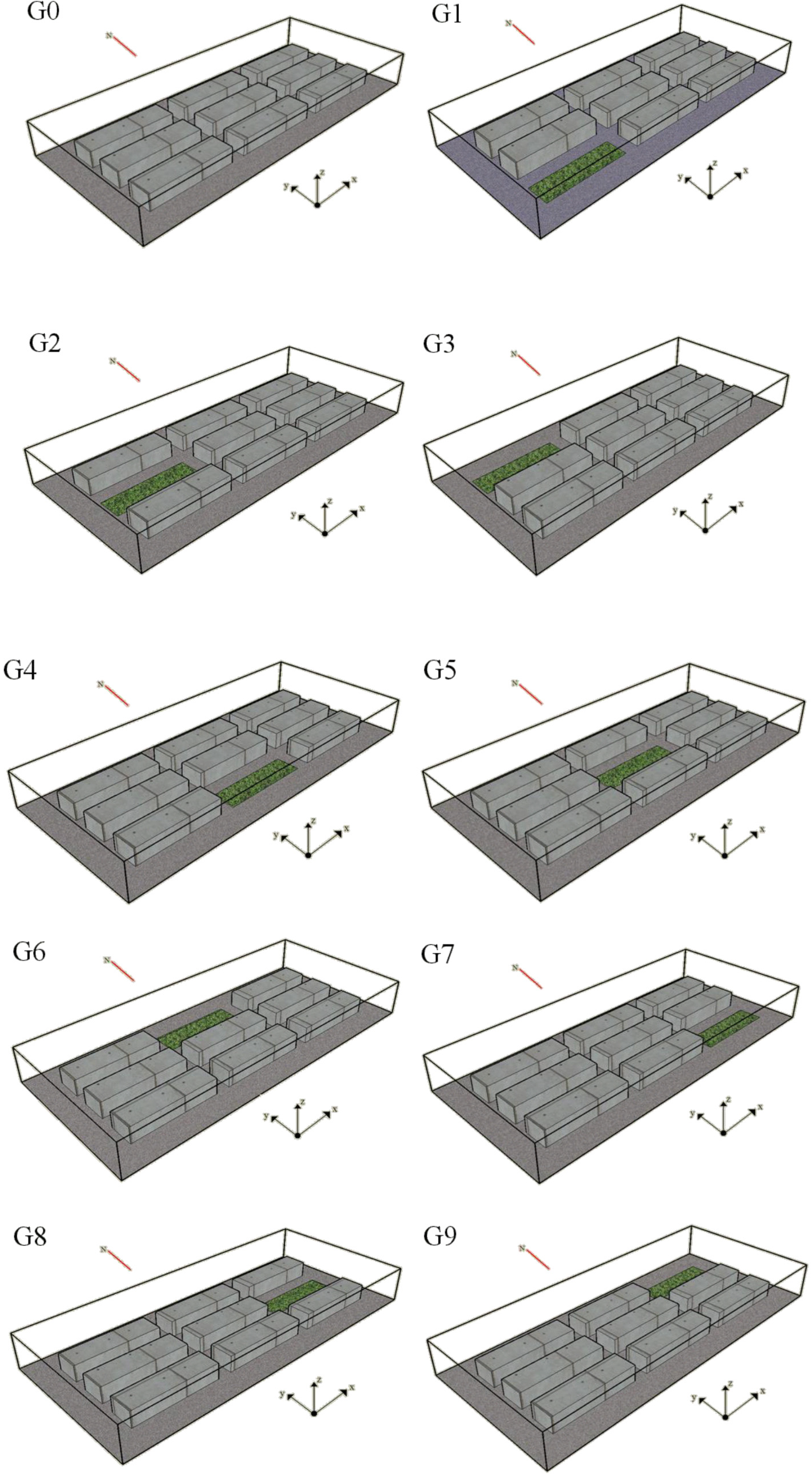
The location of green spaces in a land reconsolidation zone will influence the distribution of the microclimate in this zone. The green space in a city block can reduce the local average temperature to some degree.

(2)

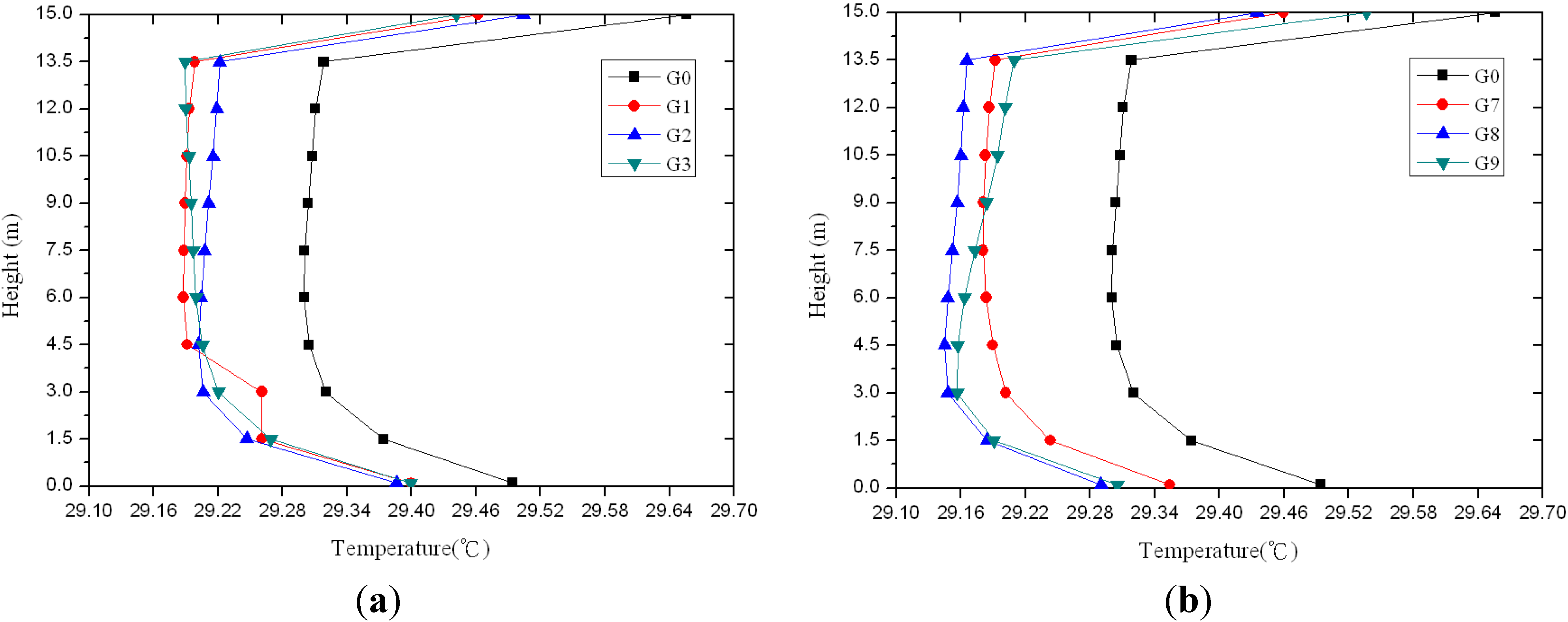
Based on the simulated climate conditions and location used in this research, a green space located in the center of this area and at the far side of the downstream area of a summer monsoon is the recommended layout to reduce the temperature at the low wind area, the average temperature of this area. In the G8 layout, the average temperature can be reduced by 0.19 °C at a height of 1.5 m above the asphalt road by using this optimal layout. The G4 layout with a green space in the center is best for reducing the highest temperature and can reduce the intensity of the heat effect by 0.36 °C.

(3)

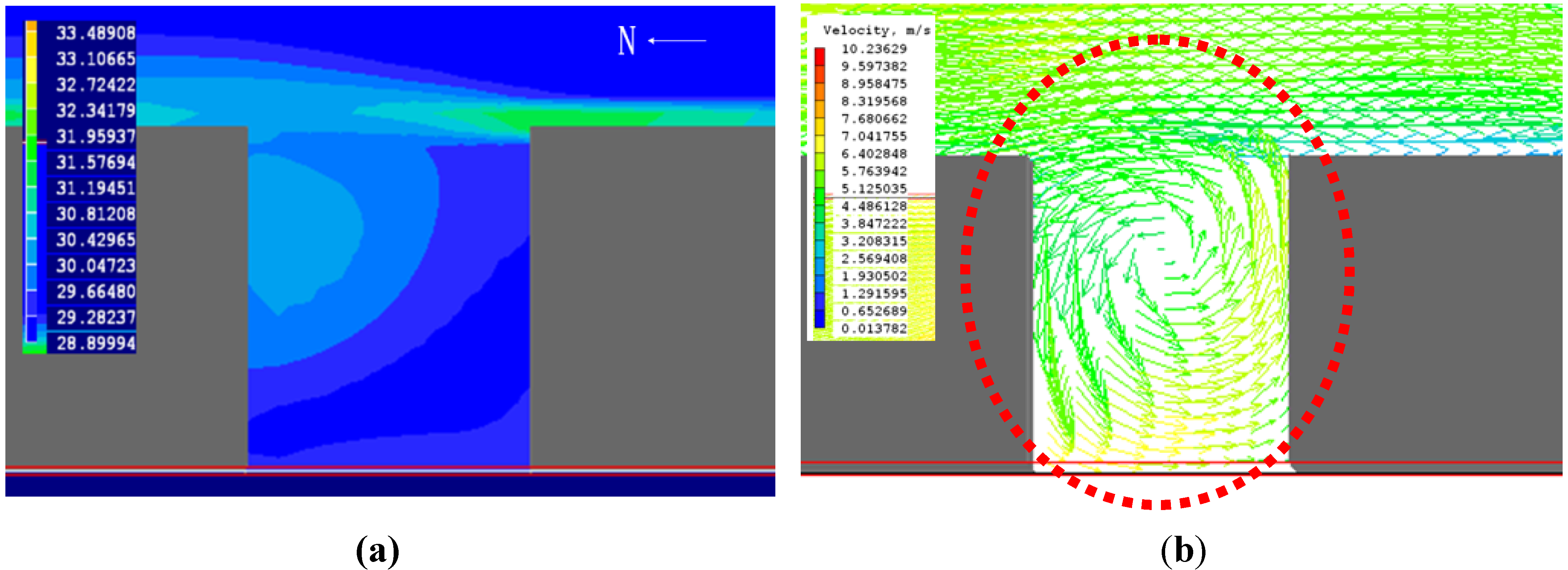
When considering where to establish a green space in a neighborhood area, factors such as the local climate, the building use conditions and the airflow patterns should be taken into consideration. In terms of the airflow pattern, from the simulation results, it can be seen that heat will accumulate in the northeastern part where there is also an area with a lower wind velocity. Therefore, before the overall site planning takes place, the airflow pattern should be fully understood, and thus the optimal green space layout can be determined.

In this study, only the heat dissipation of the air conditioner condenser and the reemission after the solar heat gain from the roofs and the road asphalt was taken into account in the calculations. Future work to address effects of radiation reflected from the surrounding walls of the city block, solar radiation absorbed and re-emitted as long wave radiation from the adjacent surfaces, potential convective heat transfer effects, evapotranspiration effects around the green area, etc. is definitely needed, which are necessary steps towards developing more reliable predictive tools for the heat island research.

References

1. Mirzaei, P.; Haghighat, F. Approaches to urban heat island-abilities and limitations. Build. Environ. 2010, 45, 2192–2201. [Google Scholar] [CrossRef]
2. Takahashi, K.; Yoshida, H.; Tanaka, Y. Measurement of thermal environment in Kyoto city and its prediction by CFD simulation. Energy Build. 2004, 36, 771–779. [Google Scholar] [CrossRef]
3. Mirzaei, P.A.; Haghighat, F. A novel approach to enhance outdoor air quality: Pedestrian ventilation system. Build. Environ. 2010, 45, 1582–1593. [Google Scholar] [CrossRef]
4. Priyadarsini, R.; Hien, W.N.; David, C.K.W. Microclimatic modeling of the urban thermal environment of Singapore to mitigate urban heat island. Sol. Energy 2008, 82, 727–745. [Google Scholar] [CrossRef]
5. Oke, T.R. Boundary Layer Climates, 2nd ed.; Routledge: London, UK, 2002. [Google Scholar]
6. Jeong, S.Y.; Yoon, S.H. Method to quantify the effect of apartment housing design parameters on outdoor thermal comfort in summer. Build. Environ. 2012, 53, 150–158. [Google Scholar] [CrossRef]
7. Chen, H.; Ooka, R.; Huang, H.; Tsuchiya, T. Study on mitigation measures for outdoor thermal environment on present urban blocks in Tokyo using coupled simulation. Build. Environ. 2009, 44, 2290–2299. [Google Scholar] [CrossRef]
8. Synnefa, A.; Karlessi, T.; Gaitani, N.; Santamouris, M.; Assimakopoulos, D.N.; Papakatsikas, C. Experimental testing of cool colored thin layer asphalt and estimation of its potential to improve the urban microclimate. Build. Environ. 2011, 46, 38–44. [Google Scholar] [CrossRef]
9. eQUEST. DOE2.com Homepage. Available online: http://www.doe2.com (accessed on 21 September 2012).
10. Kuo, B.Y. A Study on Electricity Consumption of Residential Buildings in Taiwan [in Chinese]. M.Sc. Thesis, National Cheng Kung University, Tainan, Taiwan, 2005. [Google Scholar]
11. Lai, C.M.; Wang, Y.H. Energy-saving potential of building envelope designs in residential houses in Taiwan. Energies 2011, 4, 2061–2076. [Google Scholar] [CrossRef]
12. Chen, Q. Comparison of different k-ε models for indoor air flow computations. Numer. Heat Transf. Part B Fundam. 1995, 28, 353–369. [Google Scholar] [CrossRef]
13. Spalding, D.B. The PHOENICS Encyclopedia; CHAM Ltd.: London, UK, 1994. [Google Scholar]