3.2.1. Peak Over Threshold Extrapolation Method
In case of a peak extrapolation method, there are three different ways to extract peaks from 10 min time series: global maxima, block maxima, and peak over threshold. If global maxima is used, only the largest peak within a 10 min time series is extracted. For block maxima, the time series are divided into equally distributed time blocks and from each block the largest peak is extracted. The Peak Over Threshold (POT) method extracts several peaks in every 10 min time series. Thereby, the largest value between each successive upcrossing of the threshold is extracted. Investigations have shown that the POT method yields superior results in comparison to the other methods [
11,
12]. In the literature and in the IEC standard it is recommended to choose a threshold which is the mean value plus 1.4 times the standard deviation (
) [
4,
9]. Moreover, determining an optimal threshold can lead to better fits of the distributions [
11]. The aggregation of the peaks at each individual mean wind speed can be done by means of two procedures “fitting before aggregation” or “aggregation before fitting”. Toft
et al. [
12] showed that the “fitting before aggregation” approach yields the best results. For the extracted and aggregated peaks, local distribution functions have to be fitted for each given mean wind speed
v. In the literature, several distribution functions are used: three parameter Weibull (W3P), Weibull, normal, Rayleigh, Gumbel,
etc. However, in general a W3P distribution function is preferred for the local distributions [
5,
11,
12,
27]:
where
x is the considered load of the OWT and
τ is the length of each time series. Based on the local distribution, the short-term distribution for the maximum load within a time series of the length
τ is given as
where
is the average number of independent peaks at the mean wind speed
v within the time interval
. Then, the long-term distribution can be approximately determined by integrating over the mean wind speeds given by the density function
:
Furthermore, it is assumed that
is truncated to the interval
[
12]. Under the assumption that the individual time series are independent, the probability for the characteristic extreme load
with a recurrence period of
(years) is then defined as
The method considered in the present paper can be summarized as follows: POT extraction with a threshold
, “aggregation before fitting” and a W3P distribution to fit the local distributions. In order to ensure that the extracted peaks are independent, the independency is tested by Blum’s test [
28], which is also used by Fogle
et al. [
7]. Blum’s test uses a test statistic
B that has to be lower than a critical value
. For a significance level of 1% the critical value is
. For the different input configurations, the mean
B values are estimated for each wind speed bin. The values of the flapwise bending moment are lower than
, which is also lower than the critical value. In addition, the sample correlation coefficients
ρ are determined. It turns out that all coefficients are lower than
. Therefore, independency of the extracted flapwise bending moments can be assumed. In terms of the edgewise bending moment, bins with a low wind speed have mean
B values up to
while for higher wind speeds the mean values are also significantly lower than the critical value. The sample correlation coefficients show a similar characteristic, with correlation coefficients up to
for bins with a low wind speed and less than
for high wind speeds. For high wind speeds, it can be assumed that the extracted edgewise bending moments are independent. The independency of the extracted edgewise bending moments at low wind speeds could be improved by adding a minimum separation time between the peaks. According to Ragan and Manuel [
11], the requirement of a minimum separation time between the extracted peaks only has a small effect on the extrapolated long-term load predictions. Moreover, it would significantly reduce the amount of available data and the procedure would be more complicated. Due to this and due to the reason that the peak loads at low wind speeds have only a small effect on the extrapolated loads, no separation time is used. As already mentioned above, 30 time series of 10 min duration are available for each input configuration.
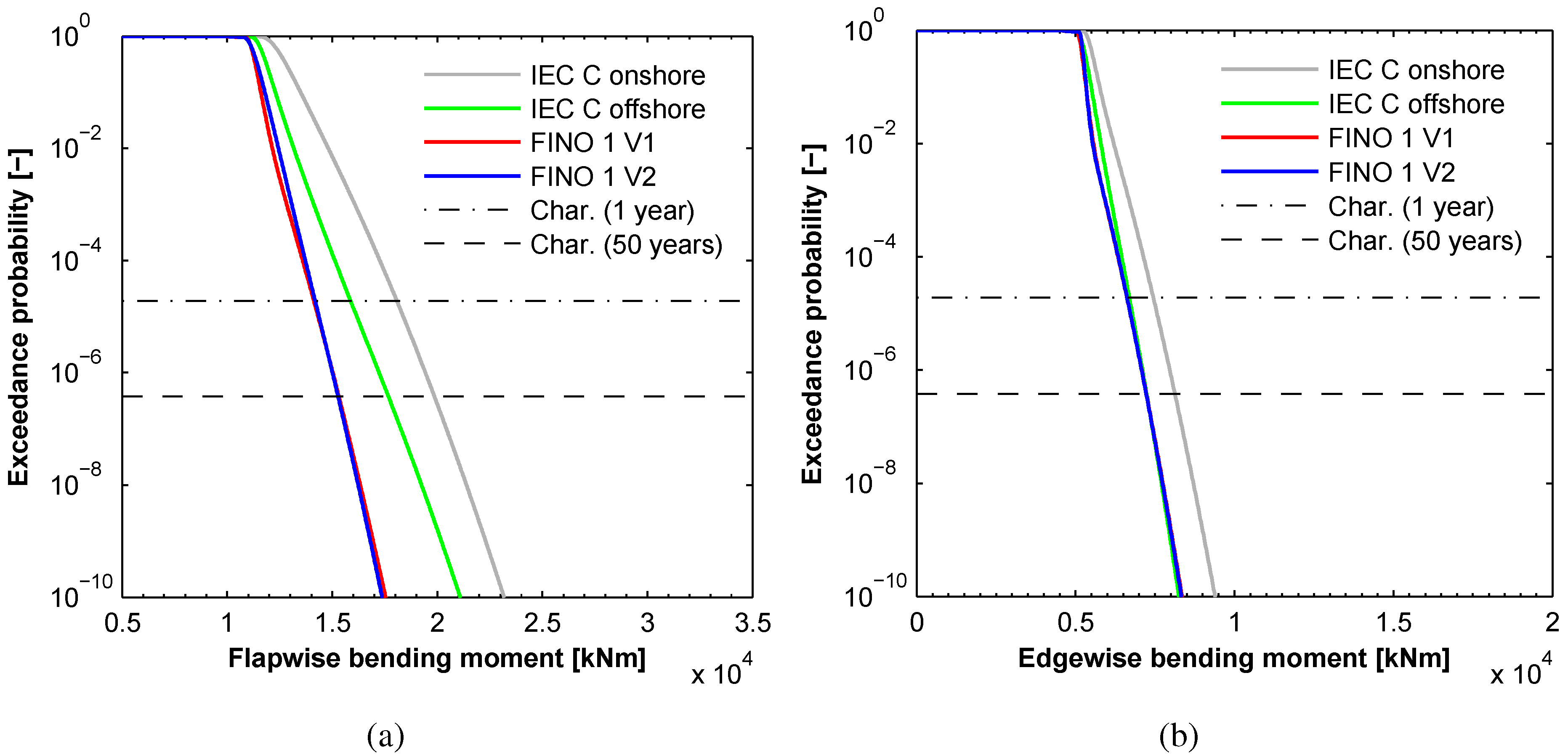
Figure 6.
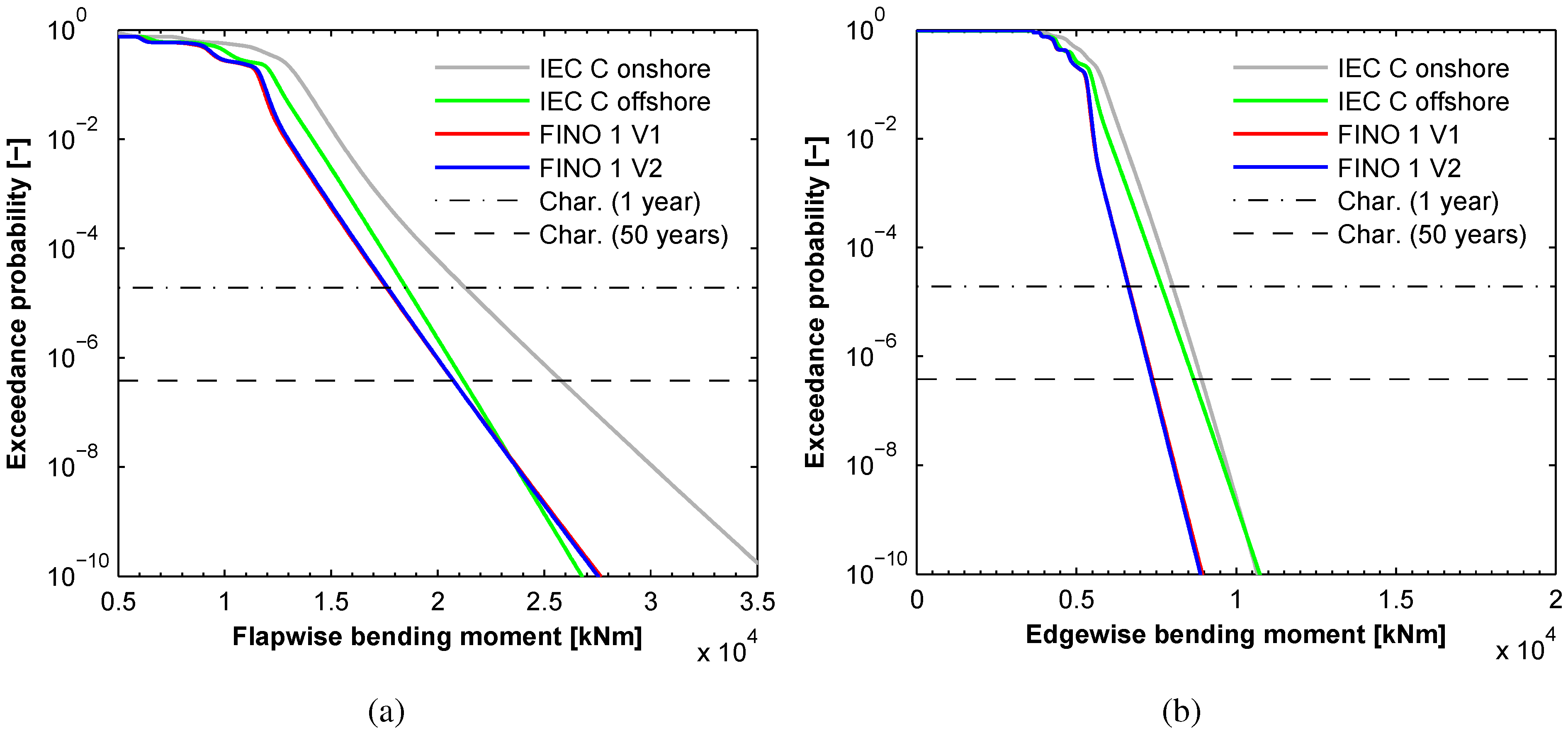
Long-term exceedance probability distribution of the bending moments at the blade root calculated by means of the POT method. (a) Flapwise; (b) Edgewise.
Figure 6.
Long-term exceedance probability distribution of the bending moments at the blade root calculated by means of the POT method. (a) Flapwise; (b) Edgewise.
Figure 6 shows the resulting long-term exceedance probability distributions of the flapwise and edgewise bending moments at the blade root. In addition to this,
Table 2 shows the characteristic extreme loads with a recurrence period of 1 year and 50 years. There are almost no differences between the characteristic extreme loads of FINO 1 V1 and V2. Therefore, the extreme loads are also more affected by the turbulence intensity than the wind shear. In comparison to the characteristic extreme flapwise bending moment (50 years recurrence period) of the FINO 1 data, the IEC C offshore value is 2% higher and the IEC C onshore value is 24% higher. In terms of the edgewise bending moment, the increases are about 17% and 21%, respectively. Typically, the edgewise bending moments are mainly dominated by gravity forces, so that such a high increase could not be expected. The fits of the local distribution functions based on the IEC C simulations are worse compared to the FINO 1 data. Especially, for the wind speed
the local distribution function significantly overestimates the tail of the extracted edgewise bending moments of the IEC C simulations (
Figure 10). This leads also to an overestimation of the characteristic extreme edgewise bending moment and therefore to a large difference between IEC C and FINO 1 results.
Table 2.
Characteristic extreme loads calculated by means of the POT method.
Table 2.
Characteristic extreme loads calculated by means of the POT method.
| | Flapwise bending moment [kNm] | Edgewise bending moment [kNm] |
|---|
| Characteristic | 1 year | 50 years | 1 year | 50 years |
|---|
| IEC C onshore | 21,292 | 25,798 | 8,023 | 8,916 |
| IEC C offshore | 18,520 | 21,204 | 7,672 | 8,672 |
| FINO 1 V1 | 17,607 | 20,735 | 6,643 | 7,386 |
| FINO 1 V2 | 17,654 | 20,739 | 6,628 | 7,358 |
3.2.2. Average Conditional Exceedance Rates
A novel extrapolation method for predicting characteristic extreme loads with a certain recurrence period is based on Average Conditional Exceedance Rates (ACER). This method was developed by Naess and Gaidai [
17,
18] and was already applied to estimate extreme wind speeds [
29] or to determine extreme loads of wind turbines [
5]. In the following a short overview is given in terms of the estimation of empirical ACER functions. For the theoretical background it is referred to [
5,
17,
18,
29]. If
M simulated time series of the length
τ with
N extracted peaks are available, the exceedance rate can be empirically estimated by counting the number of conditional exceedances of the load level
η. The exceedance rate, which is conditioned on the
previous non-exceedances, can be empirically estimated for each time series by [
5]:
The variables
Q and
R describe an ergodic process and a time-invariant non-ergodic field, respectively. Furthermore,
is a random function
for
and
, where
denotes the peak value of the load series at a certain time and
is the indicator function of a random process
. Based on the empirically estimated exceedance rate (Equation 11), the ACER function for
M simulations is given by:
In order to approximate the empirically estimated ACER function, an appropriate asymptotic extreme value distribution of the Gumbel type with four parameters is used [
5]:
To reach better fits of the ACER function, a tail marker
is introduced, because exceedance rates at small load levels
η are not very representative for the extreme value distribution. The optimal values of the parameters
a,
b,
c and
q can be determined by minimizing the following mean square error function [
5,
18,
29]:
where
L is the number of considered load levels and
is a weight factor based on the 95% confidence interval
of the empirically estimated ACER function, which puts more emphasis on the more reliable data points with a low level of uncertainty:
Based on Equation 16, load levels with small relative confidence intervals of the empirically estimated ACER function get higher weight factors. As described in [
5,
18,
29], the minimization of Equation 15 can be done by using the Levenberg–Marquardt least square optimization method. The success of this optimization highly depends on the chosen start values of the individual parameters. A procedure to define reasonable initial guesses is presented for example in [
5].
In the present study, the only ergodic variable in
Q is the mean wind speed
v. Due to reasons of simplicity, the time-invariant non-ergodic variables
R, which represent the model and statistical uncertainty, are not taken into account [
5]. Then, the reduced distribution function for the long-term extreme loads
is given as
The expected value with respect to the mean wind speed
v can be determined by
In the present study, the expected value is calculated numerically based on 12 different mean wind speeds. For each wind speed 30 time series with 10 min duration are used, where each is divided into 20 time intervals with the same length. Then, the maximum peak in each interval is extracted. The results of Toft
et al. [
5] show that there are only small differences between the unconditional ACER (
) and conditional ACER functions (
;
) for the tail values. Because of this, only unconditional exceedance rates (
) are used in the following. In order to fit the ACER function, the tail marker is chosen by means of a simple optimization. In only a few cases the optimization performs poorly. Then, the tail marker is defined manually in the way that the remaining data is sufficient for the fit.
Figure 7 shows the resulting long-term exceedance probability distributions of the flapwise and edgewise bending moments at the blade root. Furthermore, in
Table 3 the corresponding characteristic extreme loads are presented with a recurrence period of 1 year and 50 years, respectively. Corresponding to the results of the POT methods, almost no differences can be identified between the characteristic extreme loads of FINO 1 V1 and V2. Compared to the data based on FINO 1, the characteristic flapwise bending moments (50 years recurrence period) of the IEC standard conditions are 15% to 30% higher. The characteristic edgewise bending moments of FINO 1 and IEC C offshore are nearly identical. Compared with that, the characteristic edgewise bending moment of IEC C onshore is about 12% higher.
Figure 7.
Long-term exceedance probability distribution of the bending moments at the blade root calculated by means of the ACER method. (a) Flapwise; (b) Edgewise.
Figure 7.
Long-term exceedance probability distribution of the bending moments at the blade root calculated by means of the ACER method. (a) Flapwise; (b) Edgewise.
Table 3.
Characteristic extreme loads calculated by means of the ACER method.
Table 3.
Characteristic extreme loads calculated by means of the ACER method.
| | Flapwise bending moment [kNm] | Edgewise bending moment [kNm] |
|---|
| Characteristic | 1 year | 50 years | 1 year | 50 years |
|---|
| IEC C onshore | 18,078 | 19,861 | 7,447 | 8,126 |
| IEC C offshore | 15,876 | 17,669 | 6,692 | 7,234 |
| FINO 1 V1 | 14,129 | 15,313 | 6,617 | 7,227 |
| FINO 1 V2 | 14,189 | 15,276 | 6,619 | 7,223 |
3.2.3. Convergence Criteria
As mentioned above, based on the results of Fogle
et al. [
7] and Moriarty
et al. [
9], for each input configuration (mean wind speed, turbulence intensity, wind shear exponent) 30 simulations are performed. In general it can be stated that more simulations lead to a larger number of extracted peaks, which can help to get a better fit for the tail of the short-term distributions. This will reduce the uncertainty of the aggregated long-term distribution and also of the extrapolated extreme loads [
7]. In order to show that 30 simulations for each input configuration are sufficient and an acceptable uncertainty level is reached, a convergence criterion in form of a normalized confidence interval is used:
where the denominator
represents the
p-quantile load of the empirical short-term load distribution and the numerator represents the
confidence interval on the
p-quantile load. The variable
q describes the maximum acceptable percentage error permitted on the normalized confidence interval [
7]. In the IEC standard 61400-1 [
4]
q is 15%, and in case of global maxima, the normalized 90% confidence interval on the 84th-quantile load is considered. If more load peaks are extracted within a 10 min time series by means of the block maxima or the POT method, the
p-quantile with
must be chosen, where
is the average number of independent peaks at the mean wind speed
v within the 10 min time interval. In the IEC standard [
4], the bootstrap method is one of the recommended methods to estimate the confidence interval on the
p-quantile load. Based on the original sample (extracted load peaks), the bootstrap method creates a large number of random resamplings with replacement which have the same size as the original sample. The
p-quantile can be determined for each newly created sample and based on these the confidence interval can be estimated. An extensive description of the bootstrap method is given in [
30]. In the present study, 5000 resamplings are used to estimate the 90% confidence intervals on the
p-quantile loads. The bootstrap method is based on a random process, therefore the bootstrap simulation is repeated 10 times for each mean wind speed.
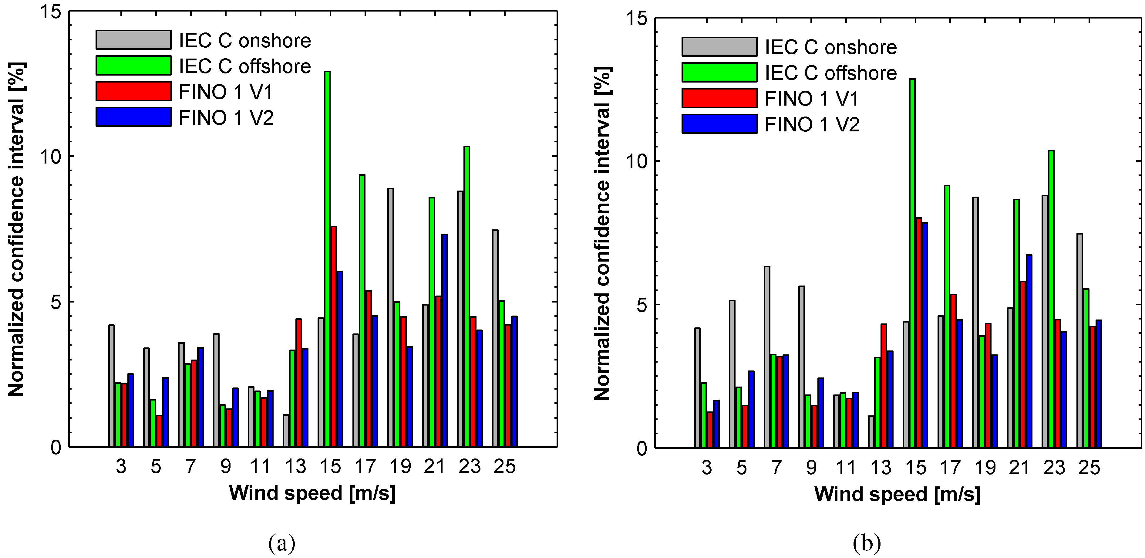
Figure 8 shows the mean values of the normalized 90% confidence intervals on the
p-quantile of the flapwise bending moments for the POT and ACER method.
Figure 8.
Normalized 90% confidence interval on the p-quantile of the flapwise bending moment based on (a) POT; (b) ACER method.
Figure 8.
Normalized 90% confidence interval on the p-quantile of the flapwise bending moment based on (a) POT; (b) ACER method.
For all wind speeds, the mean values of the confidence interval are lower than 15%. Due to a low standard deviation in all cases, the maximum value of the confidence interval is also lower than 15%. The normalized confidence intervals of the edgewise bending moments are lower than 10%. Thus, it can be assumed that 30 simulations are sufficient in the present study.
3.2.4. Comparison
The results of the POT method and the ACER method (
Table 2 and
Table 3) show that the characteristic extreme loads obtained by the POT method are generally larger. Furthermore, the characteristic of the long-term exceedance distributions differ significantly (compare
Figure 6 and
Figure 7). In comparison to the ACER method, an increase of the flapwise bending moment leads to minor changes in the exceedance probability based on the POT method. Reasons for this are the differences of the POT and ACER method itself as well as the different distribution functions used. The three parameter Weibull distribution is generally preferred in literature for the POT method and also yields consistently good results in the present study. According to [
5], the Gumbel distribution is used for the ACER method. In
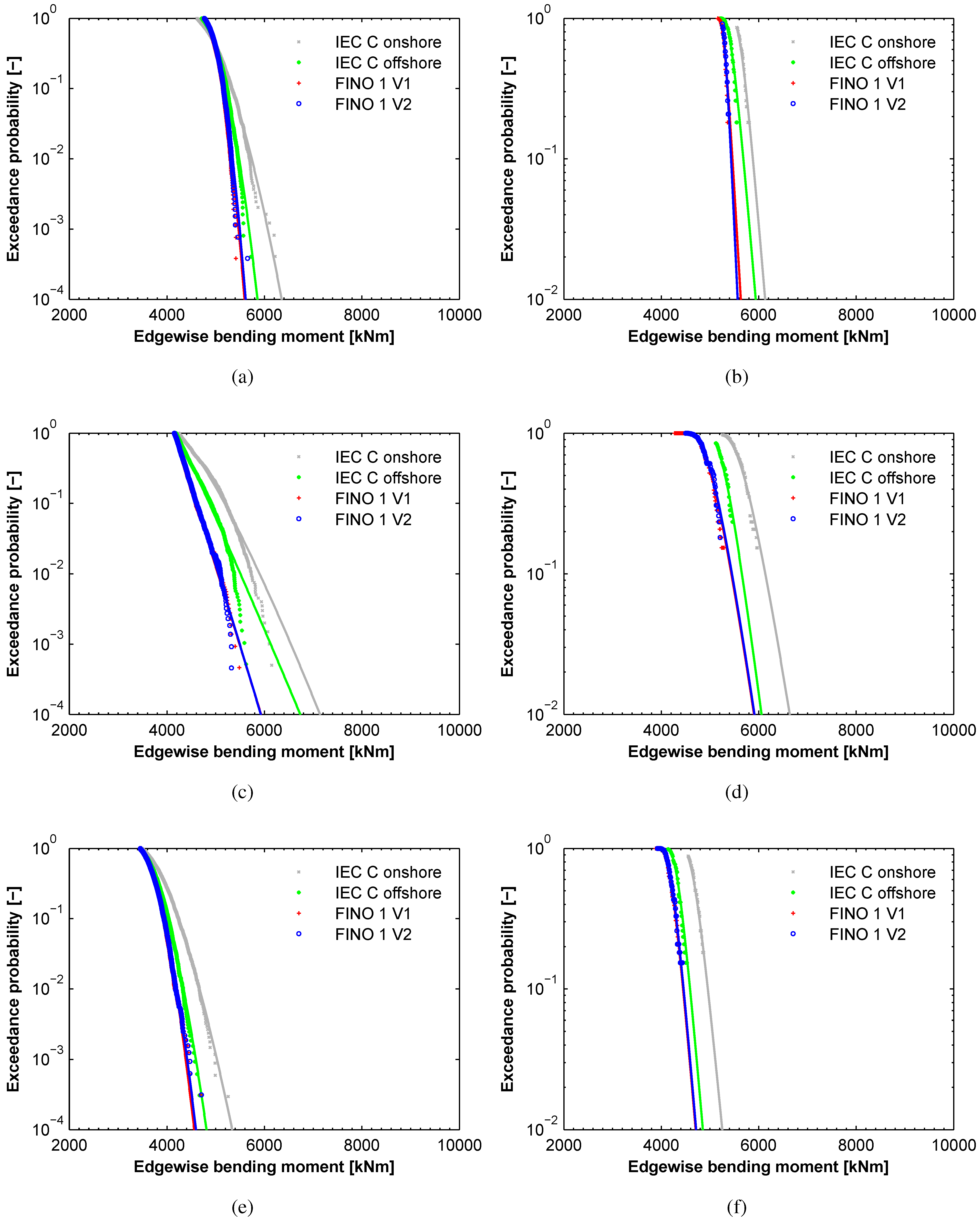
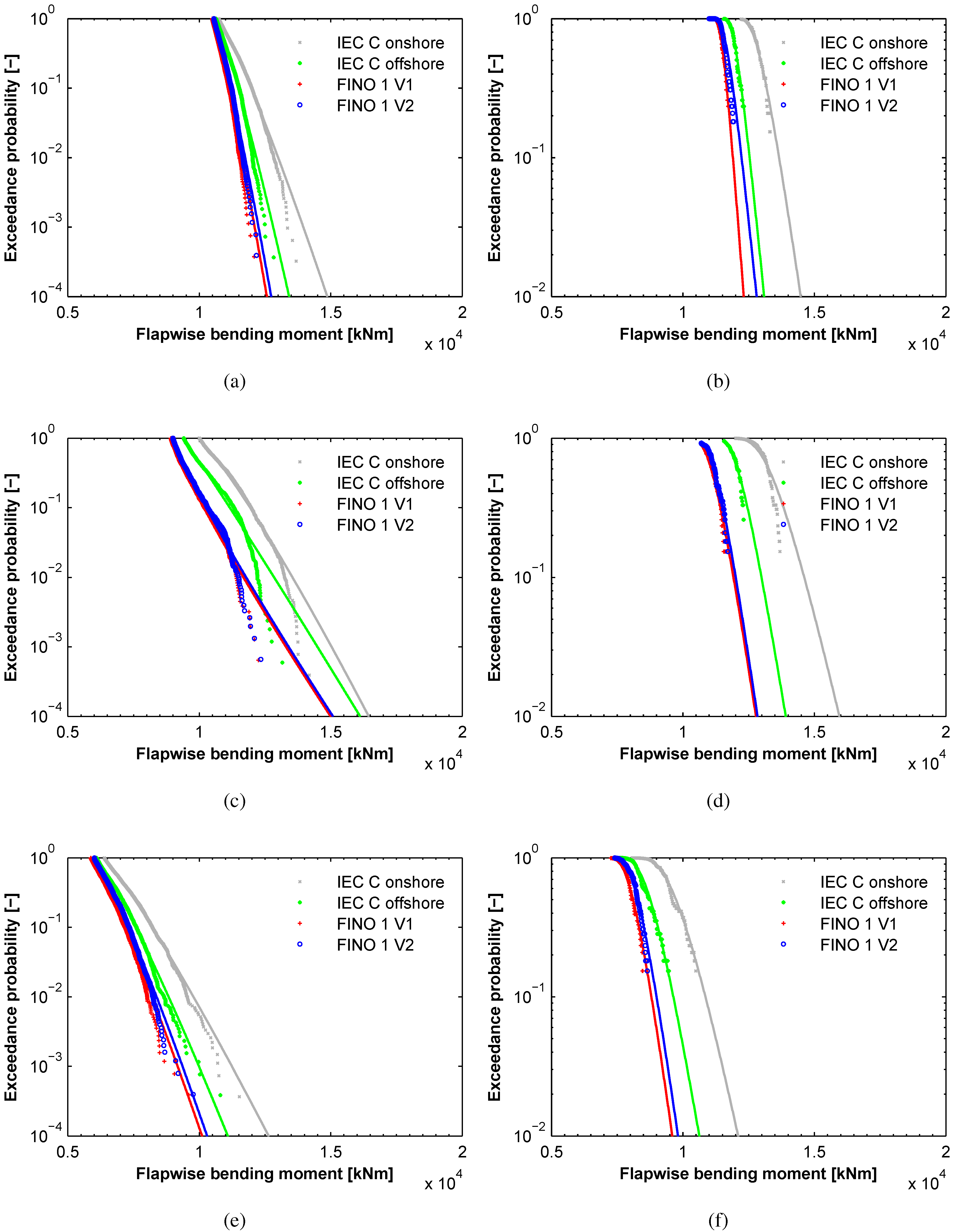
Figure 9, it is shown that the data fits of the POT method are worse compared with fits of the ACER method. Except for the wind speed
, the empirical ACER functions are fitted very well. In contrast to that, the local distribution functions overestimate the tail of the extracted data based on the POT method. In
Figure 10, this is also seen for the local distributions of the edgewise bending moments. Therefore, it is assumed that the characteristic loads obtained by means of the ACER method are more plausible.
Figure 9.
Local exceedance probability distribution for the flapwise bending moment at the blade root (please notice the different scales of the y-axis). (a) POT, ; (b) ACER, ; (c) POT, ; (d) ACER, ; (e) POT, ; (f) ACER, .
Figure 9.
Local exceedance probability distribution for the flapwise bending moment at the blade root (please notice the different scales of the y-axis). (a) POT, ; (b) ACER, ; (c) POT, ; (d) ACER, ; (e) POT, ; (f) ACER, .
Figure 10.
Local exceedance probability distribution for the edgewise bending moment at the blade root (please notice the different scales of the y-axis). (a) POT, ; (b) ACER, ; (c) POT, ; (d) ACER, ; (e) POT, ; (f) ACER, .
Figure 10.
Local exceedance probability distribution for the edgewise bending moment at the blade root (please notice the different scales of the y-axis). (a) POT, ; (b) ACER, ; (c) POT, ; (d) ACER, ; (e) POT, ; (f) ACER, .

