A Numerical Corrosion Rate Prediction Method for Direct Assessment of Wet Gas Gathering Pipelines Internal Corrosion

Abstract

The paper introduces a numerical internal corrosion rate prediction method into the internal corrosion direct assessment (ICDA) process for wet gas gathering pipelines based on the back propagation (BP), the genetic algorithm (GA) and BP, and the particle swarm optimization and BP artificial neural networks (ANNs). The basic data were collected in accordance with the terms established by the National Association of Corrosion Engineers in the Wet Gas Internal Corrosion Direct Assessment (WG-ICDA) SP0110, and the corrosion influencing factors, which are the input variables of the ANN model, are identified and refined by the grey relational analysis method. A total of 116 groups of basic data and inspection data from seven gathering pipelines in Sichuan (China) are used to develop the numerical prediction model. Ninety-five of the 116 groups of data are selected to train the neural network. The remaining 21 groups of data are chosen to test the three ANNs. The test results show that the GA and BP ANN yield the smallest number of absolute errors and should be selected as the preferred model for the prediction of corrosion rates. The accuracy of the model was validated by another 54 groups of excavation data obtained from pipeline No. 8, whose internal environment parameters are similar to those found in the training and testing pipelines. The results show that the numerical method yields significantly better absolute errors than either the de Waard 95 model or the Top-of-Line corrosion model in WG-ICDA when applying the approach to specific pipelines, and it can be used to investigate a specific pipeline for which the data have been collected and the ANN has been developed in WG-ICDA SP0110.

1. Introduction

Wet natural gas is defined as natural gas saturated with water or other natural gas liquids. It is often transported from a production facility to a main transmission pipeline or gas processor through gas gathering pipelines inside the gas fields. However, wet gas pipelines are significantly more prone to suffer instances of liquid condensation and deposition than dry gas pipelines. As a result, a risk of internal pipeline corrosion may result from the presence of corrosive components in the condensate liquid [1,2,3].

The detection and evaluation of corrosion defects are of great importance for the safe operation of wet gas gathering pipelines. For wet gas, the most commonly used corrosion evaluation criterion is the Wet Gas Internal Corrosion Direct Assessment SP0110 (WG-ICDA SP0110) [4], which is published by the National Association of Corrosion Engineers (NACE). This criterion proposes a systematic approach for prioritizing the inspection segments so that the results from the inspection of some sections can be used to make inferences regarding the entire pipeline, and the corrosion rate of the pipeline is one of the prioritized determinations of the inspection segments.

In the criterion, the corrosion rate can be calculated using any industrially accepted internal corrosion prediction model (ICPM), such as the Anderko model [5], the Crolet model [6], the de Waard model [7], or the Norsok model [8]. However, the results of the respective ICPMs may deviate from the realistic corrosion rates when the internal environmental parameters of the inspection segments are not within the scope of the prediction model. Then, the selected excavation points based on the ICPM’s results may not provide an effective means for identifying areas that are “above average” in terms of weight loss.

There are several wet gas gathering pipelines in the particular region of interest in Sichuan Province, China. During the ICDA processing of seven pipelines, the commonly used de Waard 95 model [3] and the Top-of-Line corrosion model [4] were selected to predict the internal corrosion rates, and 116 points from seven pipelines were excavated and inspected. However, the absolute errors between the model results and inspection data were not satisfactory. For the de Waard 95 model, 86 out of 116 excavation points (74.13% of the total) yielded absolute errors greater than 0.05 mm/a. For the Top-of-Line corrosion model, 95 of 116 excavation points (81.90% of the total) gave absolute errors greater than 0.05 mm/a, and 17 of 116 excavation points (14.65% of the total) had absolute errors greater than 0.1 mm/a. Hence, it is both necessary and of significant importance that an applicable model for the wet gas gathering pipelines in this specific area of the Sichuan Province be developed to be able to obtain effective ICDAs for those pipelines.

Based on the use of artificial neural networks (ANNs), this paper develops an effective numerical method to evaluate the corrosion rate of wet gas gathering pipelines. The applicability of the method is related to the internal environments of the pipelines, whose basic data are used to train and validate the ANN model. The applicable model is developed based on 116 groups of data and is proven to be useful for wet gas gathering pipelines which are similar to the training pipelines used in the internal environments. Thus, this method can be used for specific pipelines for which the data have been collected and the corresponding ANN has been developed in accordance with WG-ICDA SP0110.

2. The Numerical Method Used for Corrosion Prediction

The internal corrosion rate of wet gas gathering pipelines is influenced by the fluid composition, temperature, pressure, flow velocity and many other factors [9]. It is difficult to develop a theoretical model that is capable of describing the relationship between all of these factors and the associated corrosion rates. However, a variety of methods can be used to predict future data based on the historical data of the system; these methods include the statistical prediction method, artificial neural networks (ANNs) and fuzzy logic methods [10]. The ANN is a non-linear data modeling tool, and it is usually utilized to model complex statistical relationships between inputs and outputs. 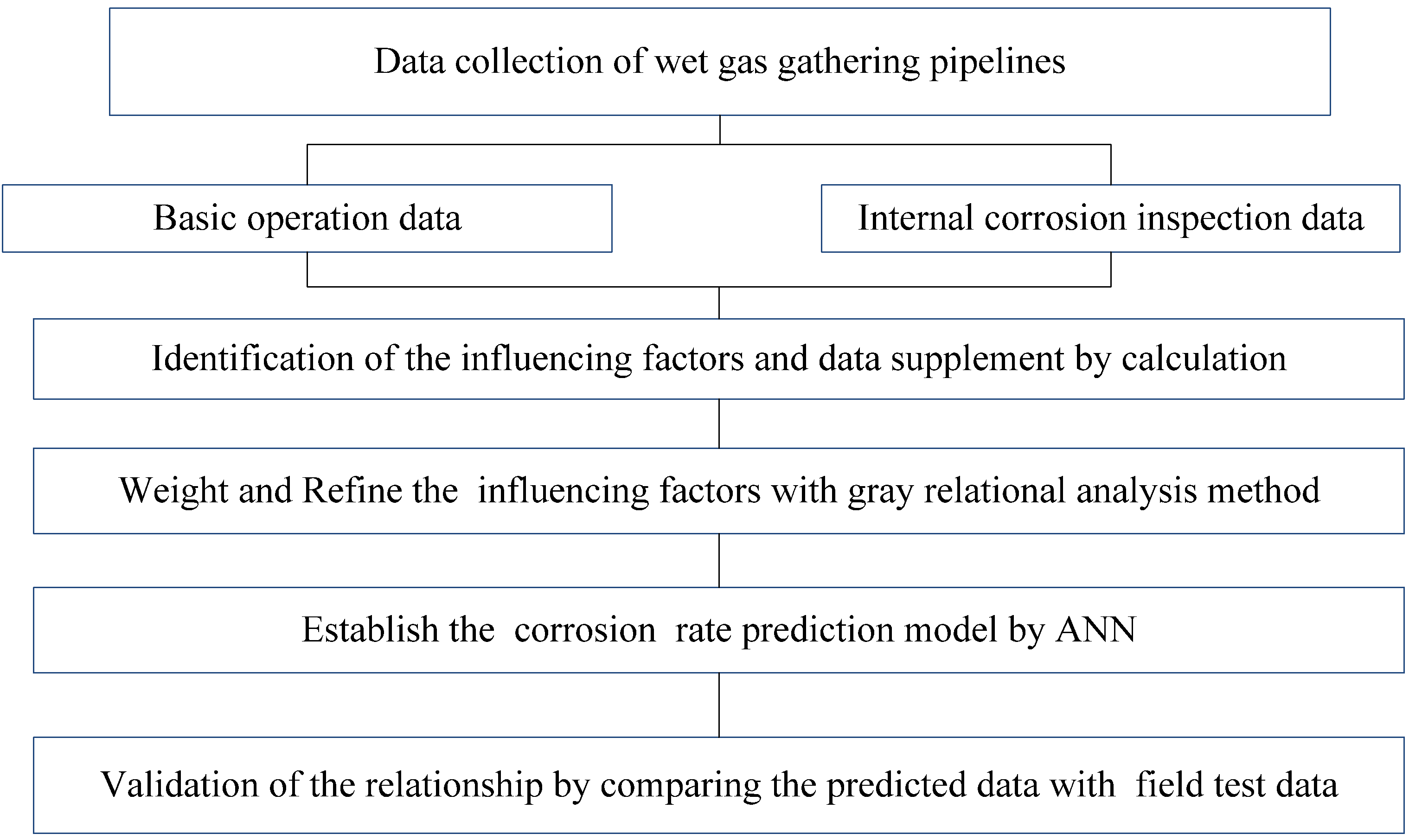Recently, researchers have applied neural network models to predictions of CO₂ corrosion in steel pipelines, and the method has been proven useful for corrosion rate prediction [11]. In this paper, ANNs also are employed to predict the internal corrosion rate of a wet gas gathering pipeline. The flow chart of internal corrosion rate prediction is shown in Figure 1. The input and output variables are critical parameters in the ANN model, and they are all discussed in the following sections.

Figure 1. The logic diagram used to establish the method.

Figure 1. The logic diagram used to establish the method.

2.1. Data Collection from the Wet Gas Gathering Pipelines

The ANN numerical prediction model must be trained by the input and output data. To accomplish this, a significant amount of historical and current correlated data from a wet gas gathering pipeline must be collected. The minimum amount of data for this purpose is proposed in WG-ICDA SP0110. The data are divided into two sets, including the specific basic data and the specific internal corrosion inspection data, which are listed in Table 1 [4].

Table 1. The specific data that must be collected.

The specific basic data:

The system design information, including the length of the pipeline, the size of the pipeline, the pipeline material, the operation time, the design transmission capacity, the design pressure, and the pipeline geographical distribution;

The pipeline mapping data, including the pipeline elevation map;

The operating history, e.g., the inlet pressure, the inlet temperature, the outlet pressure, the outlet temperature, the flow, the maximum and minimum flow rates, and the corresponding fluctuations, shutdowns, and starts in the pipeline operation in recent years;

The fluid composition, e.g., the composition of the gas and the liquid, the pH, the presence of H2S, CO2 and O2, and water and the solid contents of the fluids;

The pipeline operation, e.g., the transmission process (the pressurization, the thermal insulation), the transmission temperature, the pressure, the flow rate;

The anti-corrosion measures, including the mitigation currently applied to control the internal corrosion or the mitigation that has been applied historically;

Other known and documented causes of internal corrosion, such as microbiologically influenced corrosion (MIC);

The specific internal corrosion inspection data:

The previous records of internal corrosion, including the previous inspection reports, the previous failures, the maintenance records, etc;

The recent three years’ worth of internal corrosion inspection data from the assessed pipelines detected by long-range ultrasonic testing (LRUT), automated ultrasonic testing (AUT) and manual ultrasonic testing (UT); additionally, the source of the inspection data should be the official data provided by the certified detection organization.

Table 1. The specific data that must be collected.

The specific basic data:

The system design information, including the length of the pipeline, the size of the pipeline, the pipeline material, the operation time, the design transmission capacity, the design pressure, and the pipeline geographical distribution;

The pipeline mapping data, including the pipeline elevation map;

The operating history, e.g., the inlet pressure, the inlet temperature, the outlet pressure, the outlet temperature, the flow, the maximum and minimum flow rates, and the corresponding fluctuations, shutdowns, and starts in the pipeline operation in recent years;

The fluid composition, e.g., the composition of the gas and the liquid, the pH, the presence of H2S, CO2 and O2, and water and the solid contents of the fluids;

The pipeline operation, e.g., the transmission process (the pressurization, the thermal insulation), the transmission temperature, the pressure, the flow rate;

The anti-corrosion measures, including the mitigation currently applied to control the internal corrosion or the mitigation that has been applied historically;

Other known and documented causes of internal corrosion, such as microbiologically influenced corrosion (MIC);

The specific internal corrosion inspection data:

The previous records of internal corrosion, including the previous inspection reports, the previous failures, the maintenance records, etc;

The recent three years’ worth of internal corrosion inspection data from the assessed pipelines detected by long-range ultrasonic testing (LRUT), automated ultrasonic testing (AUT) and manual ultrasonic testing (UT); additionally, the source of the inspection data should be the official data provided by the certified detection organization.

2.2. Definitions of the Influencing Factors and the Data Supplement

(1) Identification of the Influencing Factors

Metal corrosion always occurs on the interface between the metal part and the corroding media. The properties of the fluid media, the material, the internal surface state and the operation influence the corrosion rate of the pipeline [12,13]. The specific internal corrosion influence factors for wet gas gathering pipelines are shown in Table 2.

Table 2. The internal corrosion influencing factors that should be identified.

The metal material and the surface state of the metal:
The metal material		The surface film of the metal
The nature of the fluid:
Water content (Liquid holdup)	Inhibitor	pH value	Hydrogen sulfide
Carbon dioxide	Dissolved oxygen	The amount of salts	Solid particles
Surface tension	Microorganisms, including sulfate-reducing bacteria
Density, e.g., density of gas, density of liquid
Viscosity, e.g., liquid viscosity, gas viscosity
The pipeline operating parameters:
The temperature	e.g., the inner wall temperature, the fluid temperature, the gas temperature, the liquid temperature
The rate	e.g., the gas flow rate, the liquid flow rate, the superficial gas flow rate, the superficial liquid flow rate, the deposition rate, the erosion velocity ratio
The heat transfer	e.g., the heat transfer from the inner pipe wall to the fluid, the heat transfer coefficient of the inner wall, the thermal conductivity of the gas and the liquid
The surface shear stress	e.g., the gas-max wall shear stress, the liquid-max wall shear stress
The flow pattern	The turbulence intensity		The pressure

Table 2. The internal corrosion influencing factors that should be identified.

The metal material and the surface state of the metal:
The metal material		The surface film of the metal
The nature of the fluid:
Water content (Liquid holdup)	Inhibitor	pH value	Hydrogen sulfide
Carbon dioxide	Dissolved oxygen	The amount of salts	Solid particles
Surface tension	Microorganisms, including sulfate-reducing bacteria
Density, e.g., density of gas, density of liquid
Viscosity, e.g., liquid viscosity, gas viscosity
The pipeline operating parameters:
The temperature	e.g., the inner wall temperature, the fluid temperature, the gas temperature, the liquid temperature
The rate	e.g., the gas flow rate, the liquid flow rate, the superficial gas flow rate, the superficial liquid flow rate, the deposition rate, the erosion velocity ratio
The heat transfer	e.g., the heat transfer from the inner pipe wall to the fluid, the heat transfer coefficient of the inner wall, the thermal conductivity of the gas and the liquid
The surface shear stress	e.g., the gas-max wall shear stress, the liquid-max wall shear stress
The flow pattern	The turbulence intensity		The pressure

(2) Supplemental Data

Limited by the range of measure items, only a portion of the influencing factor data can be obtained by field testing, and the remaining data must be supplemented by calculation. Many certified software packages, such as SPT Group OLGA 7.1, are capable of carrying out these calculations. Of course, the calculation results must be verified by the field tested data before use.

2.3. Weighting and Refinement of the Influencing Factors with Grey Relational Analysis

One of the most important decisions in the development of an artificial neural network model is the selection of input variables for the model. The grey relational analysis (GRA) method is used here to weight and refine the most important factors from Table 2 [14,15]. The weights reflect the relative importance among the factors. The factors with larger weights are selected as the input variables in the numerical prediction model [16]. The procedure of the GRA weight calculation method is summarized as follows: the internal corrosion inspection data reflect the behavior of the system characteristics. First, set all of the corrosion inspection rates as the reference sequence:

$$X_0=\{x_0(1),x_0(2),...,x_0(n)\}$$

(1)

where n is the total number of inspected data.

The system characteristics are influenced by the internal corrosion factors. Second, set the influencing data as a comparison sequence:

$$X_i=\{x_i(1),x_i(2),...,x_i(n)\}$$

(2)

where i = 1,2,…,m, and m is the total number of factors. Equation (2) represents an m × n matrix. Each column represents a group of influencing factors.

Some of the factors have different units of measurement. The extreme difference normalization method is used to convert the factors into a non-dimensional state [14]. Then, all of the factors’ values are limited from 0 to 1.

The correlation coefficient is used to state the correlation degree between the parameter in one group comparison sequence and the corresponding reference parameter. Here, the correlation coefficient is defined as:

$${\eta }_i(k)=\frac{\underset{j}{\text{min}} \underset{l}{\text{min}} \left|x_0(l)-x_j(l)\right|+P \underset{j}{\text{max}} \underset{l}{\text{max}} \left|x_0(l)-x_j(l)\right|}{\left|x_0(k)-x_i(k)\right|+P \underset{j}{\text{max}} \underset{l}{\text{max}} \left|x_0(l)-x_j(l)\right|}$$

(3)

where l = 1,2,…,n, and n is the total number of inspected data; j = 1,2,…, m, and m is the total number of influencing factors. k = 1,2,…,n; and $\left|x_0(k)-x_i(k)\right|$ is the absolute difference between the i^th factor in the k^th group of the influencing data and the k^th corrosion rate. $\underset{j}{\text{min}} \underset{l}{\text{min}} \left|x_0(l)-x_j(l)\right|$ is the minimum difference of all of the $\left|x_0(l)-x_j(l)\right|$; $\underset{j}{\text{max}} \underset{l}{\text{max}} \left|x_0(l)-x_j(l)\right|$ is the maximum difference of all of the $\left|x_0(l)-x_j(l)\right|$; and P is the discrimination coefficient, 0 < p <1, commonly used as p = 0.5.

The correlation coefficient only expresses the degree of correlation at each inspection point between the reference sequence and the comparison sequence. To understand the overall correlation degree of all inspection points, the correlation degree is defined as:

$$r_i=\frac{1}{n}{\displaystyle \sum _{k=1}^n{\eta }_i(k)}$$

(4)

Finally, the weights of the influencing factors can be obtained. The factors with relatively larger weights are selected as the input variables.

2.4. Establishment of the Internal Corrosion Numerical Prediction Model

The ANN is composed of a number of neuron layers. The input layer is fed with the selected input variables and passes them into the hidden layers in which the processing task takes place. Finally, the output layer receives the information from the last hidden layer and sends the results to an external source. In the model, the number of layers, the number of neurons in each layer, the weights between the related neurons and the threshold are the critical parameters. The weights and the threshold are obtained by training. The training of neural networks is a complex task of great importance [17].

One of the most popular training algorithms is the back propagation (BP) technique. Recently, many researchers have introduced intelligent optimization methods, such as the genetic algorithm (GA) [18] and particle swarm optimization (PSO) [19], into BP neural network training. Their achievements also showed that the hybrid training technique has advantages over the BP neural network. All of the algorithms, including the BP, GA and BP, PSO and BP ANNs are applied to establish the model, and the applicability of each model is evaluated. The most accurate technique is selected as the numerical prediction method applied in the internal corrosion direct assessment of the wet gas gathering pipelines in the specific area.

It should be noted that the BP technique uses the BP neural network as the numerical prediction method; in GA and BP, the BP neural network is used as the basic numerical prediction method and the genetic algorithm is used as the optimization method; in PSO and BP, the BP neural network is used as the basic numerical prediction method and the particle swarm optimization technique is used as the optimization method.

2.5. Validation of the Model

The field test corrosion rate gathered from the excavation points of the gathering pipelines is applied to validate and evaluate the effectiveness of the numerical prediction model. The excavation points should be detected in detail by a certified operator or organization, and the internal corrosion damage should be recorded carefully, including the shape, area, size and clock orientation. Additionally, it may be necessary to use color cameras to record data [20].

The measured corrosion rate values are established based on the original thickness of the pipe as well as the inspection data. The differences between these values are divided by the operational years to yield the numerical expression of the corrosion rate of the pipeline. A comparison of the measured corrosion rate values and the prediction results demonstrates the applicability of the numerical method.

3. Application of the Numerical Method

As introduced above, there are several wet gas gathering pipelines in the particular region of interest in Sichuan Province, China. A total of 116 groups of data, including the influencing factors as well as the inspection corrosion rates from seven pipelines, are used to develop the application model, and another 54 groups of data from the No. 8 pipeline are used to validate the model.

3.1. Step 1: Collection of the Basic Data

(1) The basic Data

The basic data of seven wet gas gathering pipelines are listed in Table 3, Table 4 and Table 5.

Table 3. The basic data on the seven gathering pipelines.

Basic parameter	No. 1	No. 2	No. 3	No. 4	No. 5	No. 6	No. 7
Pipe material	20 #	20#	20#	20#	20#	20#	20#
Pipe size, mm	Φ159 × 8	Φ108 × 6	Φ108 × 6	Φ108 × 6	Φ108 × 6	Φ108 × 6	Φ219 × 8
Mileage, km	12.26	2.69	2.82	2.47	2.16	3.52	8.41
Operation time, a	1994	2004	2005	2004	2005	2003	1991
Design transmission capacity, m3/d	30 × 104	10 × 104	20 × 104	7 × 104	10.4 × 104	15 × 104	40 × 104
Design pressure, MPa	6.4	6.4	6.4	6.4	6.4	6.4	6.4
Cathodic protection	Yes	No	Yes	No	No	Yes	Yes
Internal coating	No	No	No	No	No	No	No
Gas transmission capacity, m3/d	28.2 × 104	1.2 × 104	7.07 × 104	13.1 × 104	2.9 × 104	5.0 × 104	21 × 104
Ambient temperature, °C	15	15	15	15	15	15	15
Inlet pressure, MPa	5.1	2.1	2.8	5.4	2.1	2.1	5.0
Inlet temperature, °C	28	28	28	28	28	28	28
Outlet pressure, MPa	3.2	1.8	2.5	4.9	1.8	1.8	3.7
Outlet temperature, °C	25	25	25	25	25	25	26

Note: In Table 3, the pipe material 20# represents 20 Gauge steel in the USA; Φ159 × 8 represents the external diameter of the pipeline (159 mm) and the wall thickness (8 mm).

Table 3. The basic data on the seven gathering pipelines.

Basic parameter	No. 1	No. 2	No. 3	No. 4	No. 5	No. 6	No. 7
Pipe material	20 #	20#	20#	20#	20#	20#	20#
Pipe size, mm	Φ159 × 8	Φ108 × 6	Φ108 × 6	Φ108 × 6	Φ108 × 6	Φ108 × 6	Φ219 × 8
Mileage, km	12.26	2.69	2.82	2.47	2.16	3.52	8.41
Operation time, a	1994	2004	2005	2004	2005	2003	1991
Design transmission capacity, m3/d	30 × 104	10 × 104	20 × 104	7 × 104	10.4 × 104	15 × 104	40 × 104
Design pressure, MPa	6.4	6.4	6.4	6.4	6.4	6.4	6.4
Cathodic protection	Yes	No	Yes	No	No	Yes	Yes
Internal coating	No	No	No	No	No	No	No
Gas transmission capacity, m3/d	28.2 × 104	1.2 × 104	7.07 × 104	13.1 × 104	2.9 × 104	5.0 × 104	21 × 104
Ambient temperature, °C	15	15	15	15	15	15	15
Inlet pressure, MPa	5.1	2.1	2.8	5.4	2.1	2.1	5.0
Inlet temperature, °C	28	28	28	28	28	28	28
Outlet pressure, MPa	3.2	1.8	2.5	4.9	1.8	1.8	3.7
Outlet temperature, °C	25	25	25	25	25	25	26

Note: In Table 3, the pipe material 20# represents 20 Gauge steel in the USA; Φ159 × 8 represents the external diameter of the pipeline (159 mm) and the wall thickness (8 mm).

Table 4. The gas composition of pipelines No. 1, No. 2, No. 6 and No. 7.

Composition	No. 1	No. 2	No. 6	No. 7
CH4	96.850	96.280	94.770	95.220
C2H6	0.260	0.200	0.190	0.200
C3H8	0.040	0.030	0.003	0.010
C4H10+	0.008	0.200	0.004	0.004
CO2	0.800	0.590	1.840	0.910
H2S	1.750	1.720	2.100	2.150
N2	0.280	1.103	1.030	1.470
He	0.017	0.015	0.049	0.020
O2 + Ar	0.200	0.020	0.020	0.020

Table 4. The gas composition of pipelines No. 1, No. 2, No. 6 and No. 7.

Composition	No. 1	No. 2	No. 6	No. 7
CH4	96.850	96.280	94.770	95.220
C2H6	0.260	0.200	0.190	0.200
C3H8	0.040	0.030	0.003	0.010
C4H10+	0.008	0.200	0.004	0.004
CO2	0.800	0.590	1.840	0.910
H2S	1.750	1.720	2.100	2.150
N2	0.280	1.103	1.030	1.470
He	0.017	0.015	0.049	0.020
O2 + Ar	0.200	0.020	0.020	0.020

Table 5. The compositions of pipelines No. 3, No. 4, and No. 5.

Pipeline	Relative density	G/L	H2S content, %	CO2 content, %
No. 3	0.573	67358:1	1.760	1.050
No. 4	0.587	126582:1	1.730	0.810
No. 5	0.570	29000:1	2.130	1.440

Note: In Table 5, G/L represents the ratio of gas volume to liquid volume.

Table 5. The compositions of pipelines No. 3, No. 4, and No. 5.

Pipeline	Relative density	G/L	H2S content, %	CO2 content, %
No. 3	0.573	67358:1	1.760	1.050
No. 4	0.587	126582:1	1.730	0.810
No. 5	0.570	29000:1	2.130	1.440

Note: In Table 5, G/L represents the ratio of gas volume to liquid volume.

(2) The internal Corrosion Inspection Data

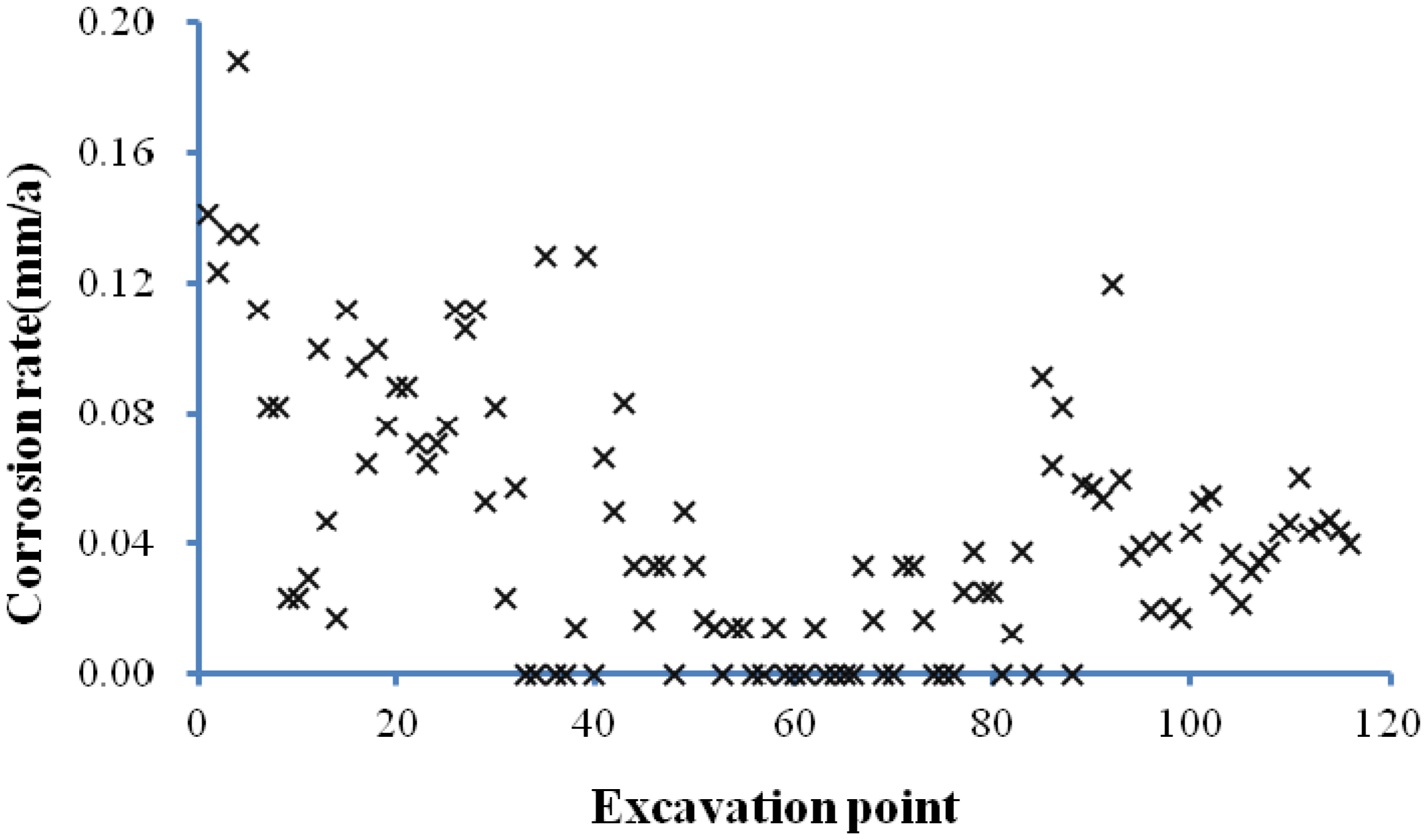
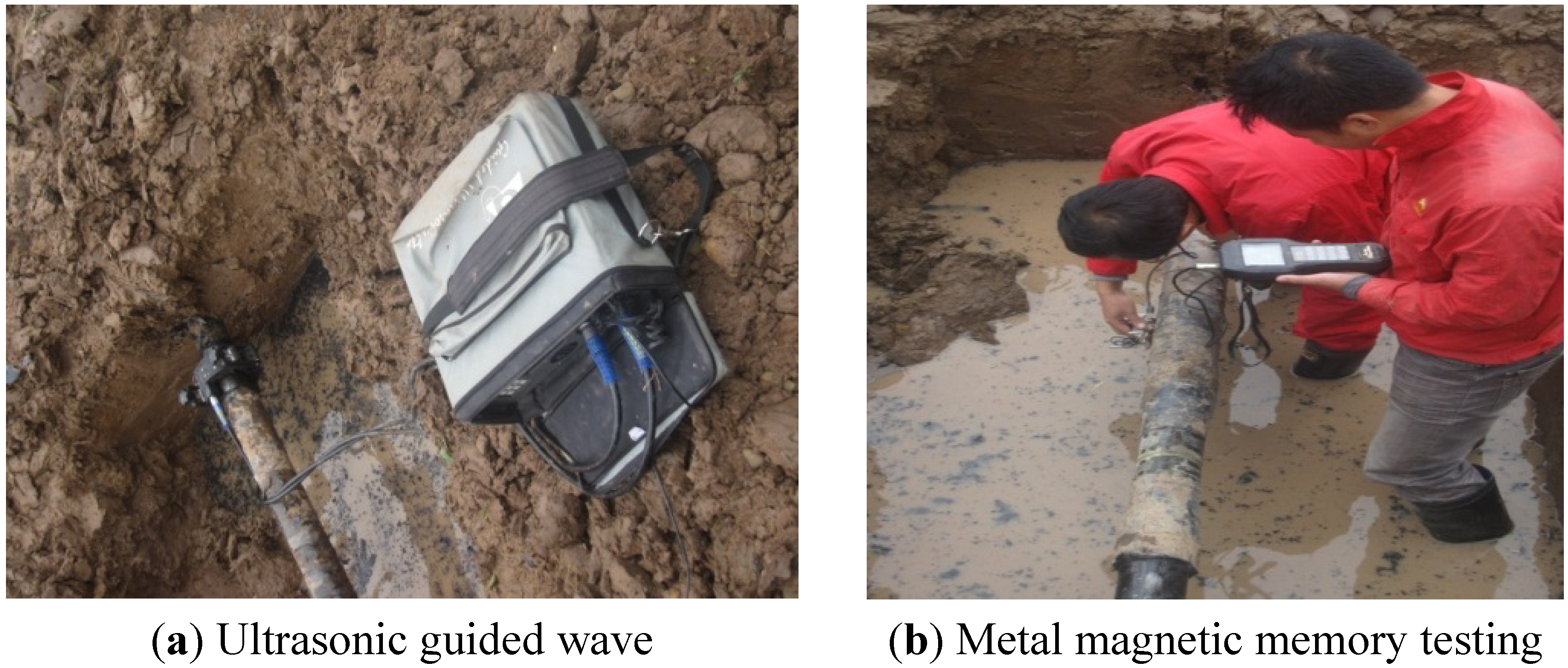
Ultrasonic guided wave and metal magnetic memory testing were applied to obtain the internal corrosion data from the pipelines. The verified internal corrosion inspection data for the seven pipelines in the region are shown in Table 6. The 116 internal corrosion rates of the pipelines are shown in Figure 2.

Table 6. The internal corrosion inspection data from the pipelines.

Pipeline	Length, km	The number of test points
No. 1	12.26	31
No. 2	2.69	9
No. 3	2.82	11
No. 4	2.47	12
No. 5	2.16	10
No. 6	3.52	11
No. 7	8.41	32
Total	34.33	116

Table 6. The internal corrosion inspection data from the pipelines.

Pipeline	Length, km	The number of test points
No. 1	12.26	31
No. 2	2.69	9
No. 3	2.82	11
No. 4	2.47	12
No. 5	2.16	10
No. 6	3.52	11
No. 7	8.41	32
Total	34.33	116

Figure 2. The detected internal corrosion rates of the pipelines. (Note: The horizontal scale is the number of each test point, as listed in Table 7. Points 1 to 31 are from the No. 1 pipeline, points 32 to 41 are from the No. 2 pipeline, etc.)

Figure 2. The detected internal corrosion rates of the pipelines. (Note: The horizontal scale is the number of each test point, as listed in Table 7. Points 1 to 31 are from the No. 1 pipeline, points 32 to 41 are from the No. 2 pipeline, etc.)

3.2. Step 2: Identification of the Influencing Factors and the Supplementary Data

(1) Identification of the Influencing Factors

The factors affecting the internal corrosion can be grouped into three sets, including the metal material and the metal surface state, the fluid nature, and the pipeline operating parameters. To simplify the development procedures in the model, the factors with similar values should not be taken into account. The similar factors are summarized in Table 7.

Table 7. The similar factors among the pipelines.

Pipe material	Pipe size (mm)	Operating pressure	Operating temperature	Acid content %
				H2S	CO2
20#	100~280	≤6.4 MPa	≤40 °C	1.7~2.3	0.5~2.0
Partial pressure ratio (PCO2/PH2S)		Methane content %	Max flow (m/s)	Flow regime (mainly)	Internal coating
0.3~0.9		≥94	4	Stratified, Slug	No

Table 7. The similar factors among the pipelines.

Pipe material	Pipe size (mm)	Operating pressure	Operating temperature	Acid content %
				H2S	CO2
20#	100~280	≤6.4 MPa	≤40 °C	1.7~2.3	0.5~2.0
Partial pressure ratio (PCO2/PH2S)		Methane content %	Max flow (m/s)	Flow regime (mainly)	Internal coating
0.3~0.9		≥94	4	Stratified, Slug	No

It can be seen that the material and internal coating of the pipelines are the same, according to Table 4 and Table 8. Hence, it is not necessary to consider these two factors in the numerical prediction methods for the area (generally, these two factors are initially considered in the pipeline design phase).

For these pipelines, the gas composition, the acid content, the total salinity and the chloride ion content change insignificantly within a certain range. The gases are all more than 94% methane, and the sulfide content ranges from 1.7% to 2.3%. In particular, the partial pressure ratios of CO₂ and H₂S are between approximately 0.3–0.9, which implies that the type of corrosion in these pipelines is predominantly hydrogen sulfide corrosion [21]. Further, for slight variations in this composition, the tendency of the gas composition to lead to corrosion in these pipelines is considered approximately the same. However, if the ratio is significantly different from 0.3 to 0.9, it is critical to obtain data from many pipelines with a sufficient distribution of data on CO₂ and H₂S so that these data can be used to correlate this important parameter. Next, the primary 21 factors should be considered, as listed in Table 8.

Table 8. The calculated internal corrosion influence factors of the pipelines.

Name	Description	Name	Description
ANGLE	pipe angle	HTK	heat transfer coefficient of inner wall
HOL	liquid holdup	QIN	heat transfer from inner pipe wall to fluid
ID	flow regime	TWS	inner wall surface temperature
PH	pH value	TCONG	thermal conductivity of gas phase
PT	pressure	TAUWG	gas-maximum wall shear stress
TM	fluid temperature	TAUWHL	liquid-maximum wall shear stress
PSID	deposition rate	USG	superficial velocity gas
SIG	surface tension	USL	superficial velocity total liquid film
ROG	density of gas	EVR	erosional velocity ratio
ROL	density of liquid	VISG	gas viscosity
VISL	liquid viscosity

Table 8. The calculated internal corrosion influence factors of the pipelines.

Name	Description	Name	Description
ANGLE	pipe angle	HTK	heat transfer coefficient of inner wall
HOL	liquid holdup	QIN	heat transfer from inner pipe wall to fluid
ID	flow regime	TWS	inner wall surface temperature
PH	pH value	TCONG	thermal conductivity of gas phase
PT	pressure	TAUWG	gas-maximum wall shear stress
TM	fluid temperature	TAUWHL	liquid-maximum wall shear stress
PSID	deposition rate	USG	superficial velocity gas
SIG	surface tension	USL	superficial velocity total liquid film
ROG	density of gas	EVR	erosional velocity ratio
ROL	density of liquid	VISG	gas viscosity
VISL	liquid viscosity

(2) Supplementary Data

The multiphase flow simulation software package SPT OLGA7.1 is utilized to supplement the values of the internal corrosion influencing factors.

3.3. Step 3: Weighting and Refinement of the Internal Corrosion Influencing Factors with Grey Relational Analysis

The weighting method, based on the grey relational analysis, is applied to refine the main influencing factors further. 116 internal corrosion inspection data from the seven pipelines are used as the reference sequence, and 116 groups of internal corrosion influence factors are used as the comparison sequence during the calculation. The calculated overall correlation degrees are listed in Table 9. The factors are sorted by the magnitude of the correlation degree.

Table 9. The degree of correlation of the internal corrosion factors of the pipelines.

Factor	HOL	HTK	PSID	USL	TAUWHL	ANGLE	TAUWG
Correlation degree	0.7603	0.7494	0.7398	0.7175	0.7095	0.7086	0.7048
Factor	TCONG	EVR	VISG	PH	TWS	TM	PT
Correlation degree	0.6953	0.6898	0.6833	0.6666	0.6627	0.6578	0.6558
Factor	ID	ROG	SIG	VISL	USG	ROL	QIN
Correlation degree	0.6546	0.6534	0.6325	0.6126	0.6126	0.5994	0.5616

Table 9. The degree of correlation of the internal corrosion factors of the pipelines.

Factor	HOL	HTK	PSID	USL	TAUWHL	ANGLE	TAUWG
Correlation degree	0.7603	0.7494	0.7398	0.7175	0.7095	0.7086	0.7048
Factor	TCONG	EVR	VISG	PH	TWS	TM	PT
Correlation degree	0.6953	0.6898	0.6833	0.6666	0.6627	0.6578	0.6558
Factor	ID	ROG	SIG	VISL	USG	ROL	QIN
Correlation degree	0.6546	0.6534	0.6325	0.6126	0.6126	0.5994	0.5616

Table 9 shows that the correlation degrees of the seven factors, including HOT, HTK, PSID, USL, TAUWHL, ANGEL, and TAUWG, are all higher than 0.7, which can be regarded as the threshold for selecting the high correlation factors [22]. These seven influencing factors for each detected position from the seven pipelines are selected as the input variables of the numerical prediction model. The corresponding internal corrosion rate data of the seven pipelines are the output variables. If the numerical prediction model is applied to other areas and pipelines, the high correlation factors may differ from those chosen in this paper.

3.4. Step 4: Establishment of the Numerical Prediction Model

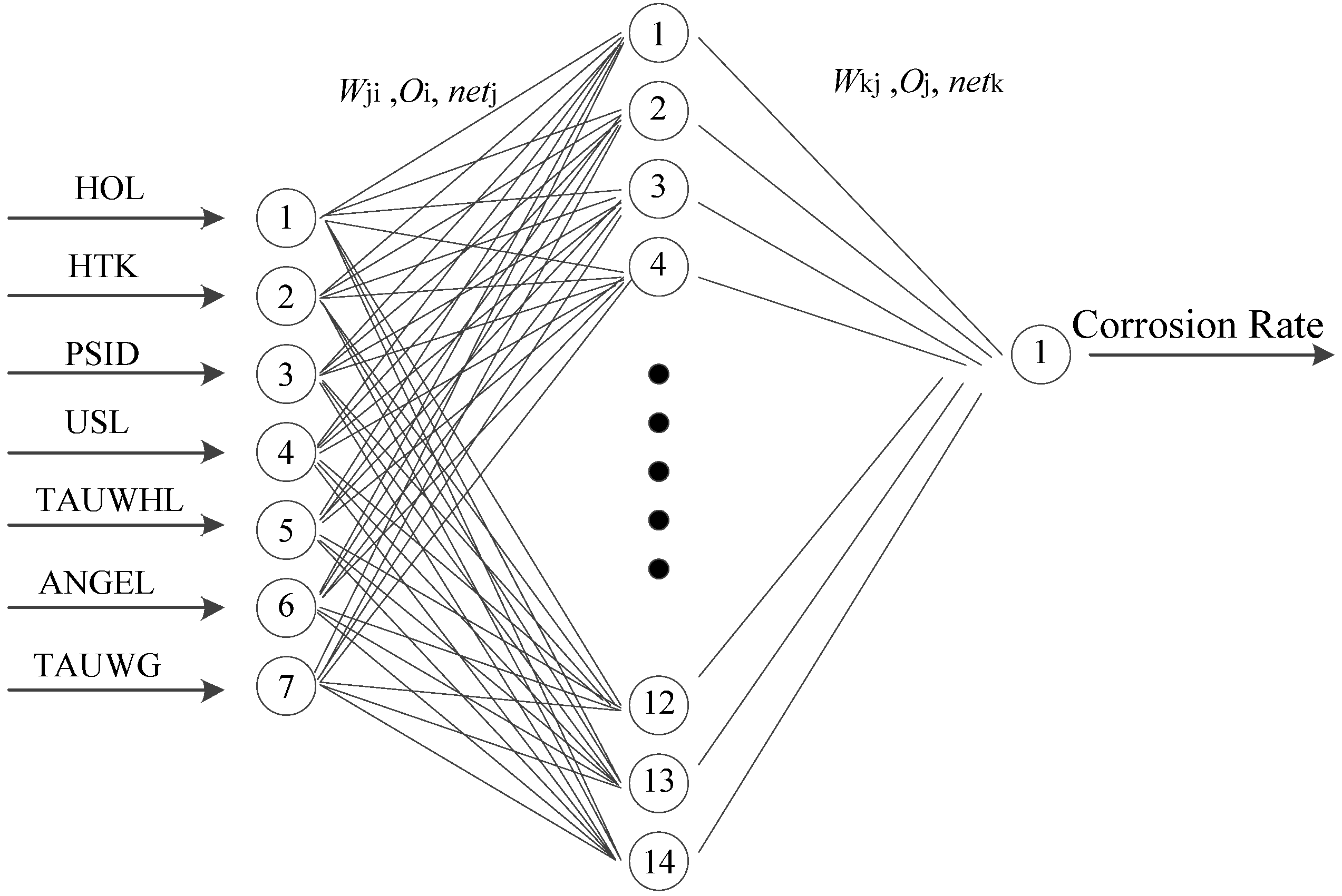
(1) The Neural Network Structure

The structure of the ANN, which is used to establish the model, is shown in Figure 3. It consists of three layers: there is one input layer with seven neurons, one hidden layer with 14 hidden neurons, and one output layer with one neuron. The 116 groups of data were divided into the training set and the testing set. Ninety-five groups of data from the No. 1, No. 2, No. 3, No. 4, and No. 7 pipelines are selected as the training set, and 21 groups of data from the No. 5 and No. 6 pipelines are selected as the test set.

Figure 3. The neural network structure.

Figure 3. The neural network structure.

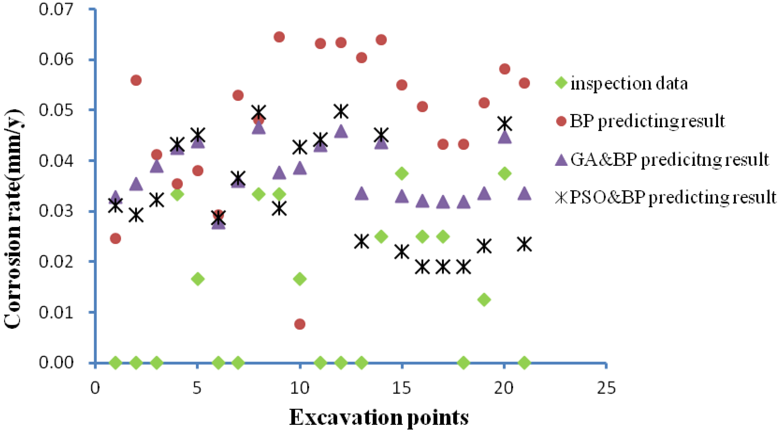
(2) Evaluation of the BP, GA&BP and PSO&BP ANNs

The three ANNs were trained with 95 groups of training data and were tested with 21 groups of basic data. The calculation results are compared with the inspection corrosion rates, as shown in Figure 4, and the absolute distribution errors of the three ANNs are listed in Table 10.

Figure 4. The predicted results of the BP, GA and BP, and PSO and BP ANNS.

Figure 4. The predicted results of the BP, GA and BP, and PSO and BP ANNS.

Table 10. The absolute errors of the corrosion rate predicted by BP, GA and BP, PSO and BP.

Error, mm/a	≥0.1	<0.1, ≥0.05	<0.05, ≥0.03	<0.03, ≥0.01	<0.01
BP error distribution	0	6	5	8	2
GA and BP error distribution	0	0	9	6	6
PSO and BP error distribution	0	0	5	12	4

Table 10. The absolute errors of the corrosion rate predicted by BP, GA and BP, PSO and BP.

Error, mm/a	≥0.1	<0.1, ≥0.05	<0.05, ≥0.03	<0.03, ≥0.01	<0.01
BP error distribution	0	6	5	8	2
GA and BP error distribution	0	0	9	6	6
PSO and BP error distribution	0	0	5	12	4

It can be seen from Figure 4 and Table 10 that the absolute errors of the BP ANN are all less than 0.1 mm/a and the absolute errors of the other two ANNs are both less than 0.05 mm/a. The majority of the error values of the PSO and BP ANN range between 0.01 and 0.03, and the GA and BP ANN has the most points with absolute errors less than 0.01 mm/a. Thus, the GA and BP model is selected as the best model for wet gas gathering pipeline corrosion rate prediction in Sichuan Province (China).

(3) Establishment of the Numerical Prediction Model

The weights and the threshold are shown in Table 11.

Table 11. The final weights and thresholds as determined by GA and BP.

	Wji							Bkj	Wkj	Bk
j	1	2	3	4	5	6	7	1	1	1
1	0.7871	0.1436	1.3603	1.3371	0.4841	0.8486	0.6212	0.526	–0.0553	0.5067
2	0.3528	–0.0278	0.6563	0.9863	1.0682	–0.3052	1.0161	1.1866	0.0634
3	0.5657	–0.2742	0.3858	–0.268	0.1617	–0.0597	0.366	2.3361	–0.0623
4	–0.0854	0.3601	1.1294	0.709	–0.4639	1.0013	–0.7004	–0.439	0.0349
5	–0.5838	0.9066	0.663	1.0599	–0.3253	–0.5323	0.3456	–0.3373	–0.0031
6	–0.1142	0.2516	0.1891	1.1337	0.4167	0.1137	0.9173	–0.4147	–0.0067
7	1.0394	0.2659	0.7327	–0.0903	0.0634	–0.0359	–0.172	3.6657	–0.3328
8	–0.2195	–0.3993	1.355	0.0281	0.9816	0.6192	0.3937	0.6424	–0.0199
9	–0.0504	1.3109	1.1697	2.1103	1.0558	1.4078	–0.4901	–0.5101	0.3902
10	0.9373	0.6316	0.3763	1.572	–0.0523	0.639	0.3539	–0.587	–0.1475
11	0.1309	0.3315	0.3036	0.1235	1.2292	1.5775	0.496	0.1291	0.0279
12	0.2275	1.1052	0.8768	0.3657	0.566	0.4937	–0.0061	0.3502	0.0838
13	0.2604	1.507	0.6898	1.6409	1.6911	1.3298	0.789	3.6935	–0.0664
14	–0.4708	–0.1168	0.5337	–0.4306	1.0504	–0.7916	0.1446	1.3818	–0.1402

Note: Wji is the weight of the input layer; Bkj is the threshold of the hidden layer; Wkj is the weight of the hidden layer; Bk is the threshold of the output layer; i is the neural number of the input layers; j is the neural number of the hidden layers; and k is the neural number of the output layers.

Table 11. The final weights and thresholds as determined by GA and BP.

	Wji							Bkj	Wkj	Bk
j	1	2	3	4	5	6	7	1	1	1
1	0.7871	0.1436	1.3603	1.3371	0.4841	0.8486	0.6212	0.526	–0.0553	0.5067
2	0.3528	–0.0278	0.6563	0.9863	1.0682	–0.3052	1.0161	1.1866	0.0634
3	0.5657	–0.2742	0.3858	–0.268	0.1617	–0.0597	0.366	2.3361	–0.0623
4	–0.0854	0.3601	1.1294	0.709	–0.4639	1.0013	–0.7004	–0.439	0.0349
5	–0.5838	0.9066	0.663	1.0599	–0.3253	–0.5323	0.3456	–0.3373	–0.0031
6	–0.1142	0.2516	0.1891	1.1337	0.4167	0.1137	0.9173	–0.4147	–0.0067
7	1.0394	0.2659	0.7327	–0.0903	0.0634	–0.0359	–0.172	3.6657	–0.3328
8	–0.2195	–0.3993	1.355	0.0281	0.9816	0.6192	0.3937	0.6424	–0.0199
9	–0.0504	1.3109	1.1697	2.1103	1.0558	1.4078	–0.4901	–0.5101	0.3902
10	0.9373	0.6316	0.3763	1.572	–0.0523	0.639	0.3539	–0.587	–0.1475
11	0.1309	0.3315	0.3036	0.1235	1.2292	1.5775	0.496	0.1291	0.0279
12	0.2275	1.1052	0.8768	0.3657	0.566	0.4937	–0.0061	0.3502	0.0838
13	0.2604	1.507	0.6898	1.6409	1.6911	1.3298	0.789	3.6935	–0.0664
14	–0.4708	–0.1168	0.5337	–0.4306	1.0504	–0.7916	0.1446	1.3818	–0.1402

Note: Wji is the weight of the input layer; Bkj is the threshold of the hidden layer; Wkj is the weight of the hidden layer; Bk is the threshold of the output layer; i is the neural number of the input layers; j is the neural number of the hidden layers; and k is the neural number of the output layers.

3.5. Step 5: Validation of the Model

From the basic data recorded for pipeline No.8, as shown in Table 12 and Table 13, it can be seen that this pipeline’s internal environment parameters are similar to those of the training and testing pipelines, as shown in Table 7.

Table 12. The basic data on the validation pipeline.

Pipe material	pipe size, mm	Length, km	Operation time, a
20#	Φ273 × 8	7.84	1991
Design pressure, MPa	Cathodic protection	Internal coating	Ambient temperature, °C
6.4	Yes	No	15
Inlet pressure, MPa	Inlet temperature, °C	Outlet pressure, MPa	Outlet temperature, °C
5.1	28	3.8	25
Design transmission capacity, m3/d		Gas transmission capacity, m3/d
70		57 × 104

Table 12. The basic data on the validation pipeline.

Pipe material	pipe size, mm	Length, km	Operation time, a
20#	Φ273 × 8	7.84	1991
Design pressure, MPa	Cathodic protection	Internal coating	Ambient temperature, °C
6.4	Yes	No	15
Inlet pressure, MPa	Inlet temperature, °C	Outlet pressure, MPa	Outlet temperature, °C
5.1	28	3.8	25
Design transmission capacity, m3/d		Gas transmission capacity, m3/d
70		57 × 104

Table 13. The composition of the validation pipeline.

Composition	CH4	C2H6	C3H8	C4+	CO2	H2S	N2	He	O2
Content %	94.62	0.19	0.03	0.20	1.28	2.29	1.46	0.11	0.05

Table 13. The composition of the validation pipeline.

Composition	CH4	C2H6	C3H8	C4+	CO2	H2S	N2	He	O2
Content %	94.62	0.19	0.03	0.20	1.28	2.29	1.46	0.11	0.05

Ultrasonic guided wave and metal magnetic memory testing methods were applied to develop the internal corrosion data of the No. 8 pipeline. A total of 54 excavation points along the pipeline have been selected to validate the GA and BP ANN prediction model. Additionally, the field situation of the excavation points is shown in Figure 5.

Figure 5. The excavation points of the validation pipeline.

Figure 5. The excavation points of the validation pipeline.

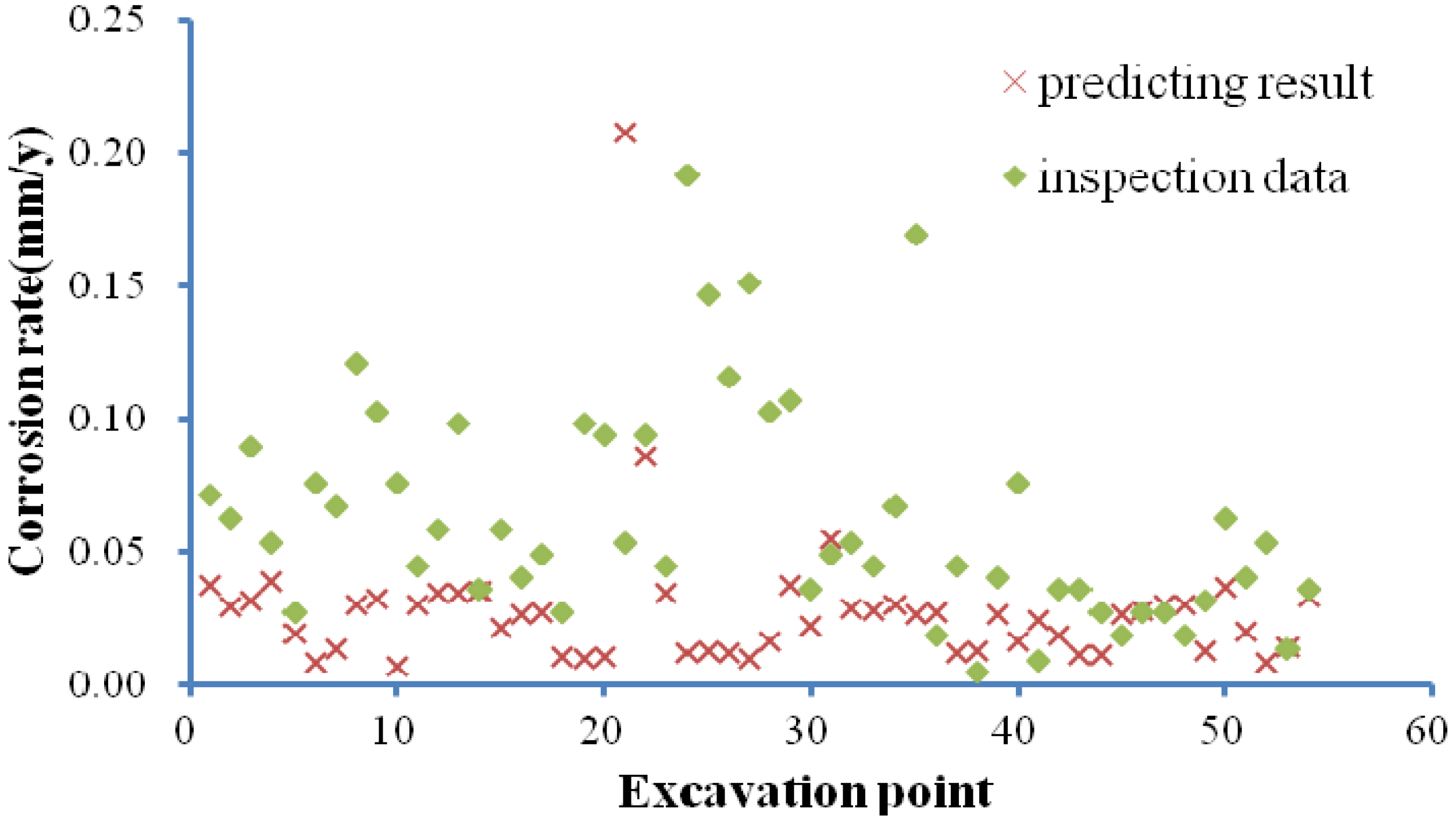
The fifty-four groups of excavation inspection data gathered from pipeline No. 8 and the corresponding results obtained by the GA and BP ANN, the de Waard 95 model and the Top-of-Line corrosion model are shown in Figure 6. The distributions of the absolute errors are shown in Table 14.

Table 14. The distribution of the prediction errors of the GA and BP for the validation pipeline.

Error, mm/a	≥2	<2, ≥1	<1, ≥0.1	<0.1, ≥0.05	<0.05, ≥0.03	<0.03, ≥0.01	<0.01
de Waard 95 model distribution	38	15	1	0	0	0	0
Top-of-Line corrosion model distribution	0	19	34	1	0	0	0
PSO and BP error distribution	0	0	6	12	6	19	11

Table 14. The distribution of the prediction errors of the GA and BP for the validation pipeline.

Error, mm/a	≥2	<2, ≥1	<1, ≥0.1	<0.1, ≥0.05	<0.05, ≥0.03	<0.03, ≥0.01	<0.01
de Waard 95 model distribution	38	15	1	0	0	0	0
Top-of-Line corrosion model distribution	0	19	34	1	0	0	0
PSO and BP error distribution	0	0	6	12	6	19	11

Figure 6. The predicted results and the inspection data of the validation pipeline.

Figure 6. The predicted results and the inspection data of the validation pipeline.

As listed in Table 14, the absolute errors of the de Waard 95 model are all greater than 0.1 mm/a, and 38 out of 54 excavation points (70.37% of the total) possess absolute errors greater than 2 mm/a. The Top-of-Line corrosion model is slightly better than the de Waard 95 model but is still not satisfactory. All of the absolute errors in the Top-of-Line model are greater than 0.05 mm/a, and 53 out of 54 excavation points (98.14% of the total) possess absolute errors greater than 0.1 mm/a. Even so, 19 points (35.18% of total) yield absolute errors greater than 1 mm/a.

In comparison, the GA and BP ANN model yields significantly more accurate error values. All of the absolute errors in this model are less than 1 mm/a, and only 18 points (33.33% of the total) possess absolute errors greater than 0.05 mm/a. The major absolute error ranges (55.55% of the total) are between 0.01 and 0.03 mm/a. This application to the No.8 pipeline demonstrates that the numerical model based on the GA and BP ANN model is significantly more accurate in comparison to the de Waard 95 model and the Top-of-Line corrosion model. Thus, the GA and BP ANN model is effective in the prediction of corrosion rates for the specific wet gas gathering pipelines in the ICDA process.

This model also can be applied to other pipelines whose internal environment parameters satisfy the parameters of Table 7. If the gas composition and pipeline operational parameters deviate too significantly from the training pipelines, the specific input variables, weights and threshold values of the numerical model should be modified accordingly [23].

4. Conclusions

This paper introduced a numerical internal corrosion rate prediction method for the internal corrosion direct assessment of wet gas gathering pipelines based on ANNs. The basic data that were used for the numerical method were determined by the NACE WG-ICDA SP0110. The influencing factors that affected the internal corrosion were identified and refined with the grey relational analysis method. The refined factors were chosen to be the input variables of the ANN model, and different algorithms, including BP, GA and BP, PSO and BP, were applied to train the model.

In the application case, 95 groups of data, including the influencing factors as well as the inspection corrosion rates from five pipelines, were used to train the application model. An artificial neural network model with seven neurons in the input layer, 14 neurons in one hidden layer and one neuron in the output layer were developed. Another 21 groups of data from two pipelines were used to test the model. The test results show a satisfactory degree of matching between the prediction corrosion rate and the inspection data, and the GA&BP ANN showed the lowest absolute errors. Thus, this model was selected as the best model for the prediction of corrosion rates.

Fifty-four groups of excavation data from the No. 8 pipeline, whose internal environment parameters are similar to those developed by the training and testing pipelines, were applied to the de Waard 95 model, the Top-of-Line corrosion model and the GA and BP ANN model. The application results show that the accuracy of the GA and BP ANN model is significantly better than that of the other two models for the specific wet gas gathering pipelines investigated. Thus, this model can be used in the study of a specific pipeline for which the data have been collected and the ANN has been developed in WG-ICDA SP0110.

References

- Mokhatab, S.; Poe, W.A.; Speight, J.G. Handbook of Natural Gas Transmission and Processing; Gulf Professional Publishing: Burlington, UK, 2006. [Google Scholar]
- Vinod, S.A.; Perry, L.R. Corrosion Detection and Monitoring—A Review. In Proceedings of the Corrosion 2000, Orlando, FL, USA, 26–31 March 2000; NACE International: Houston, TX, USA, 2000. [Google Scholar]
- De Waard, C.; Lotz, U.; Milliams, D.E. Predictive model for CO2 corrosion engineering in wet gas pipelines. Corrosion 1991, 47, 976–985. [Google Scholar] [CrossRef]
- NACE. Wet Gas Internal Corrosion Direct Assessment Methodology for Pipelines, NACE SP0110-2010; NACE International Publishing: Houston, TX, USA, 2010. [Google Scholar]
- Anderko, A. Simulation of FeCO3/FeS Scale Formation Using Thermodynamic and Electrochemical Models. In Proceedings of the Corrosion 2000, Orlando, FL, USA, 26–31 March 2000; NACE International: Houston, TX, USA, 2000. [Google Scholar]
- Crolet, J.L.; Thevenot, N.; Dugstad, A. Role of Free Acetic Acid on the CO2 Corrosion of Steels. In Proceedings of the Corrosion 1999, San Antonio, TX, USA, 25–30 April 1999; NACE International: Houston, TX, USA, 2002. [Google Scholar]
- Adsani, E.; Shirazi, S.A.; Shadley, J.R.; Rybicki, E.F. Mass Transfer and CO2 Corrosion in Multiphase Flow. In Proceedings of the Corrosion 2002, Denvor, CO, USA, 7–11 April 2002; NACE International: Houston, TX, USA, 2002. [Google Scholar]
- Norsok. CO2 Corrosion Rate Calculation Model, NORSOK Standard M-506; NORSOK Publishing: Lysaker, Norway, 2005. [Google Scholar]
- Villarreal, J.; Laverde, C.F. Carbon-steel corrosion in multiphase slug flow and CO2. Corros. Sci. 2006, 48, 2363–2379. [Google Scholar] [CrossRef]
- Zhang, G.Q.; Patuwo, B.E.; Hu, M.Y. Forecasting with artificial neural networks: The sate of art. Int. J. Forecast. 1998, 14, 35–62. [Google Scholar] [CrossRef]
- Bassam, A.; Toledo, D.O.; Hernandez, J.A. Artificial neural network for the evaluation of CO2 corrosion in a pipeline steel. J. Solid State Electrochem. 2009, 13, 773–780. [Google Scholar] [CrossRef]
- Zhang, R.; Gopal, M.; Jepson, W.P. Development of a mechanistic model for predicting corrosion rate in multiphase oil/water/gas flow. In Proceedings of the Corrosion 1997, New Orleans, LA, USA, 9–14 March 1997; NACE International: Houston, TX, USA, 1997. [Google Scholar]
- Ma, H.; Cheng, X.L.; Li, G.Q. The influence of hydrogen sulfide on corrosion of iron under different conditions. Corros. Sci. 2000, 42, 1669–1683. [Google Scholar] [CrossRef]
- Liu, S.F.; Dang, Y.G.; Fang, Z.G.; Xie, N.M. Grey System Theory and Its Applications; Sciencep Publishing: Beijing, China, 2010; pp. 62–96. [Google Scholar]
- Kang, J.; Zou, Z.H. Time prediction model for pipeline leakage based on grey relational analysis. Phys. Procedia 2012, 25, 2019–2024. [Google Scholar] [CrossRef]
- Jia, W.L.; Li, C.J.; Wu, X. Natural gas pipeline operation schemes comprehensive evaluation based on multi-hierarchy grey relational analysis. J. Grey Syst. 2011, 14, 117–123. [Google Scholar]
- Alfredo, G.; Maria, A.B.; Richard, S. Improved neural-network model predicts dewpoint pressure of retrograde gases. J. Pet. Sci. Eng. 2003, 37, 183–194. [Google Scholar] [CrossRef]
- Li, C.J.; Jia, W.L. Adaptive genetic algorithm for steady-state operation optimization in natural gas networks. J. Softw. 2011, 6, 452–459. [Google Scholar]
- Chau, K.W. Partical swarm optimization training algorithm for ANNs in stage prediction of Shing Mun River. J. Hydrol. 2006, 329, 3–4. [Google Scholar] [CrossRef]
- Liao, K.X.; Yao, Q.K.; Zhang, C. Principle and Technical Characteristics of Non-Contact Magnetic Tomography Method Inspection for Oil and Gas Pipeline. In Proceeding of International Conference on Pipelines and Trenchless Technology 2011, Beijing, China, 26–29 October 2011; pp. 1039–1048.
- Kvarekval, J.; Nyborg, R. Formation and Multilayer Iron Sulfide Films during High Temperature CO2/H2S Corrosion of Carbon Steel. In Proceedings of the Corrosion 2003, San Diego, CA, USA, 4–6 March 2003; NACE International: Houston, TX, USA, 2003. [Google Scholar]
- Zhao, J.Z.; Yu, X.C.; Li, C.J. Technology of Applicability Assessment for Defective Pipeline; Sinopec Publishing: Beijing, China, 2005. [Google Scholar]
- Srdjan, N. Key issues related to modeling of internal corrosion of oil and gas pipelines—A review. Corros. Sci. 2007, 49, 4308–4338. [Google Scholar] [CrossRef]
© 2012 by the authors; licensee MDPI, Basel, Switzerland. This article is an open access article distributed under the terms and conditions of the Creative Commons Attribution license (http://creativecommons.org/licenses/by/3.0/).