Demand Side Management for Stand-Alone Hybrid Power Systems Based on Load Identification

Abstract

Within the field of Distributed Generation (DG), stand-alone Hybrid Power Systems (HPS) are a suitable solution to provide energy to isolated facilities where the connection to a centralized grid is not affordable. The logical evolution of such systems involves the optimization of power resources and related control strategies, but also enhancements concerning the management of energy loads. This paper introduces Demand Side Management (DSM) strategies specially designed for HPS. They are applied on a real and patented HPS that consists of PV panels, a diesel generator, an inverter and a set of batteries. DSM strategies are built up on a framework of distributed endpoint devices connected to a central control application where loads are identified according to their behavior. System network components, load definitions, the control application and DSM strategies are depicted. Finally, simulations show illustrative savings achieved by the application of some of the proposed strategies.

1. Introduction

The prominent role that distributed generation (DG) has achieved in the last years has been already emphasized several times, e.g., [1,2]. The economical and operational benefits of DG are multiple [3], and the main driving forces that guarantee their continuous evolution and spread are located in stable factors, i.e., DG scientific and technical advances, restrictions on the construction of new transmission lines, increasing demands of power reliability, the consequences of the electricity market liberalization and concerns about sustainability and energy efficiency [4]. In short, we can say that DG is intended to improve the overall system efficiencies compared with centralized grid model, given that the proximity between consumers and suppliers avoids extra costs in the energy transportation, transformation and management.

Beyond the introduced benefits, small-scale electricity generation is fundamental for isolated, stand-alone scenarios, i.e., environments that are not electrified as they are located in places where electrical grid is difficult to be installed, cannot be installed, or it is not worth affording the costs; for instance, village electrification in developing countries, isolated farms, remote area electrification, movable energy box for transitory purposes, telecommunications equipment designed to work in wilderness or rural areas, etc.

Such cases make the most of sustainable systems that are autonomous or stand-alone. In this regard, HPS are usually deployed as stand-alone DG systems. HPS develop a smart combination of two or more energy conversion technologies to obtain synergistic benefits and optimized performances due to the intelligent management of resources. A typical HPS is composed by one or more renewable energy sources—e.g., photovoltaic modules (PV) or wind turbines—batteries for the energy storage and a fuel cell or a power generator (diesel) as a backup system.

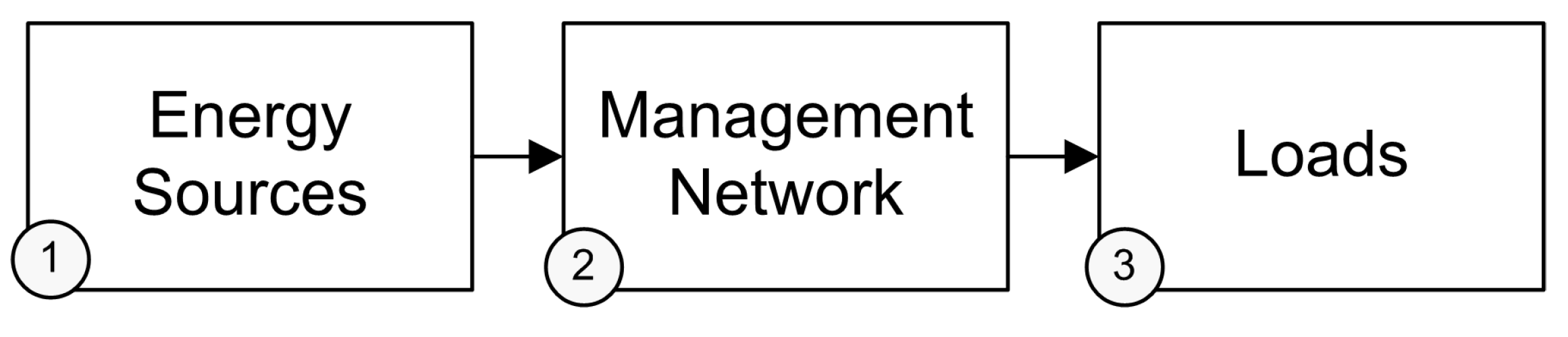
In order to make HPS competitive, the energy efficiency optimization of the whole system becomes essential. The optimization can be faced from different perspectives (Figure 1):

• By means of more efficient, smaller, cheaper, more long-lived or more sustainable energy sources. For instance, a single or dual axis solar tracker instead of fixed PV points to be advisable to improve the relationship between size and power.
• Enhancements in the management network, whether optimized equipment (e.g., inverters, low-power data and command transceivers, etc.), advanced control strategies or improved context awareness capabilities.
• In an ideal scenario, HPS work connected to a set of high efficiency energy loads (usually household appliances), which allow the maximum exploitation of the system potential.

Figure 1. Elements of a HPS network. Energy storage units (batteries) are simultaneously considered as “energy sources” and “loads”.

Figure 1. Elements of a HPS network. Energy storage units (batteries) are simultaneously considered as “energy sources” and “loads”.

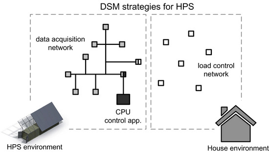
Covering points 2 and 3, some advanced systems consider optimization by empowering a conscious usage of energy loads in users (i.e., persuasive technologies [5]) and also by a smart placement of loads based on the global system status. Designs and methodologies that exploit these aspects are usually referred to as demand side management or DSM [6].

The current paper presents a DSM control system and strategies developed for a real market stand-alone HPS solution: the Wattpic Autonomous Solar Source (FSA) Container. The control system is embedded in a distributed network built on LonWorks technology in the early, prototype phase, but intended to be partially implemented using wireless networks (e.g., Zigbee, DASH7, etc.) according to the pursued features concerning mobility and flexibility. DSM development includes novelty control strategies based on load identification. In this respect, simulations carried out with models based on a real scenario show up to 28% fossil fuel reduction compared with classic performances without DSM.

2. DSM Related Literature

The concern for DSM is not new; the importance of providing solutions that influence costumers uses of electricity was already a matter of study in the 1980s. Even then, DSM were considered regardless of the kind of utility or geographic region, equally suitable “to all utilities across the country whether large or small; cooperative, municipal, or investor-owned; and urban or rural” [7].

In its broadest sense—not focusing only in DSM for DG—the main DSM techniques that have been put into practice can be summarized as follows [8]: (a) the usage of night-time electricity heating and storage heaters [9]; (b) the adoption of load limiters, i.e., loads and circuits that can be switched off when the whole demand is over a defined threshold [10]; (c) the activation of programs that boost customized or reduced pricing based on the usage of electricity, curve flattening, peak shaving or desirable time slots [11]; (d) the inclusion of smart appliances that manage their own running (disconnection, deferment, etc.) according to electricity spot price curves, demand prediction, occupancy, sleeping times, etc. [12,13]; (e) smart metering and updated feedbacks with persuasive purposes [5]; (f) in a wider scope, the management of loads and generators based on frequency regulation [14].

The special characteristics of DG, and more specifically of stand-alone microgrids based on HPS, entail constraints and limitations to the introduced approaches and also draw a very specific scenario for DSM strategies. For instance, since solar generation is concentrated in periods, to hold the demand together matching such periods instead of flattening the demand curve can be advisable (note that it is an opposite strategy to the expected for the normal grid). As far as wind generation is concerned, the localized and stochastic nature of wind also requires the application of accurate load management and control strategies able to cope with intermittency and fluctuations that can cause power and system degradation and failures [15]. An introduction to stand-alone microgrids, HPS and power management strategies (PMS) can be seen in [16]. The cooperative work of DSM and PMS are set to reach high-efficient, optimized performances.

Load shifting is one of the DSM techniques—appropriate for HPS—that has been proposed several times for the management of microgrids and DG, e.g., [17]. However, in the related literature there is a lack of canonic definitions or even proposals of DSM solutions for the specific field of stand-alone HPS, focusing preferably on the optimization of the power generation management. In any case, it is worth mentioning [18], where DSM solutions are evaluated in a HPS case study, reaching estimations of 15% electricity consumption reduction.

In this respect, the current work fills this gap presenting a set of DSM strategies suitable for stand-alone HPG.

3. FSA System

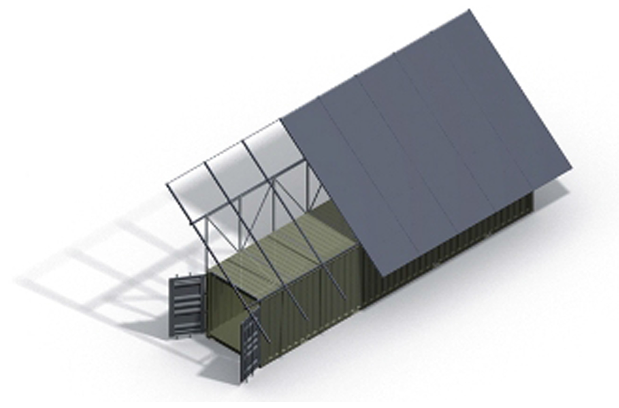
A FSA with DSM, as a real market example of DG system technology, is formed by a stand-alone HPS, a control and data acquisition network, a control application and a set of endpoint devices for the connection of electricity loads. It is devised to be a PV based plug-and-play energy system, with all its components packaged inside a standard shipping container. Figure 2 offers a graphical representation of a FSA machine.

Figure 2. Wattpic FSA Container (model without solar tracking).

Figure 2. Wattpic FSA Container (model without solar tracking).

Nowadays FSA are manufactured in three different sizes: Basic (with 60 m${}^2$ of solar surface and a power capacity of 8–11 kWp), Super (155 m${}^2$, 21–29 kWp) and Mega (300 m${}^2$, 41–56 kWp). Diesel generator, tracking, the proposed DSM and a triphasic inverter instead of monophasic are offered as optional features.

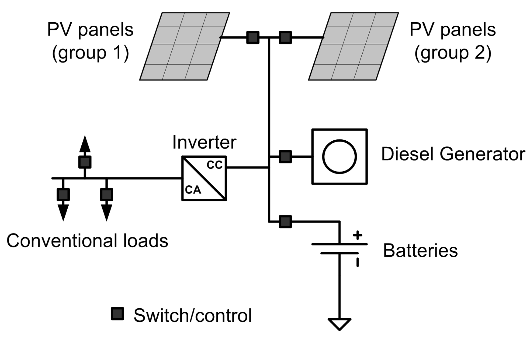
3.1. Stand-alone HPS & Data Acquisition Network

Figure 3 shows a scheme of the basic architecture of a FSA. Connected by a LonWorks network, adapted switches are controlled by an embedded CPU that executes the control application. This application rules the whole system. To accurately do that, LonWorks nodes collect information concerning the status of the different FSA elements.

By default, the main information collected in the data acquisition network is as follows:

• PV voltages and currents: $V_{g1}$, $V_{g2}$, $I_{g1}$, $I_{g2}$;
• Batteries voltage, charge and discharge currents, and state of charge (SOC): $V_{bat}$, $I_c$, $I_{dc}$, SOC;
• Generator voltage and current: $V_{gen}$, $I_{gen}$;
• Load circuit voltage and current: $V_{load}$, $I_{load}$.

Figure 3. Basic architecture of an FSA.

Figure 3. Basic architecture of an FSA.

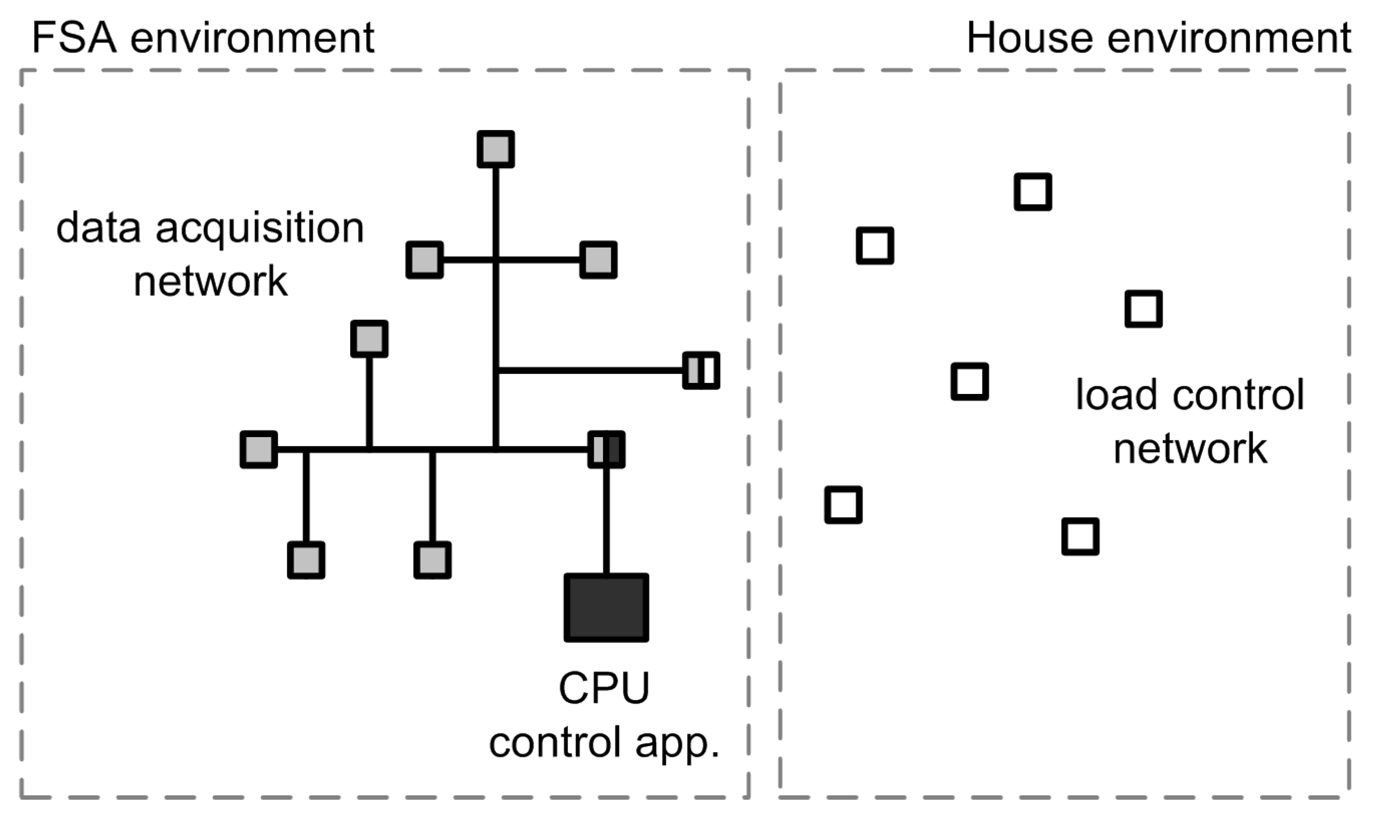
3.2. Endpoint Devices & Load Control Network

In order to apply DSM strategies, a load control network is joined to the data acquisition network as shown in Figure 4. For the sake of flexibility and mobility, the load control network is intended to be implemented by means of wireless technologies, but for prototypes and early designs the implementation has been carried out extending the normal twisted-pair wired LonWorks network.

Figure 4. Data management system scheme. Grey boxes are data acquisition devices (LonWorks) whereas white boxes are load control devices (wireless network). Note that two gateways are also present: Lon/wireless, serial/Lon.

Figure 4. Data management system scheme. Grey boxes are data acquisition devices (LonWorks) whereas white boxes are load control devices (wireless network). Note that two gateways are also present: Lon/wireless, serial/Lon.

Each load control network device is formed by: (a) a transceiver, to allow the communication within the network; (b) a control PCB, which opens and closes the power circuit to the load and collects its status; and (c) the electrical load itself. The transceiver and the control PCB forms together what is called an endpoint device.

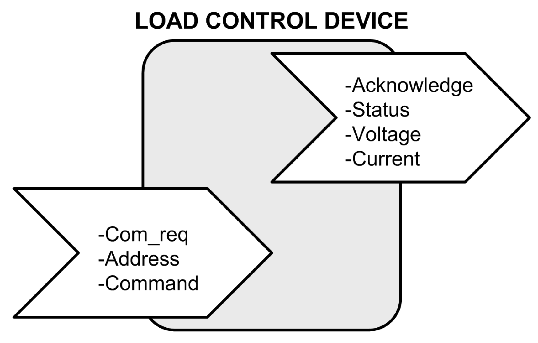
The communication corresponding to the load control devices follows a master-slave structure, it is always started by the master, i.e., the control application of the CPU, and slaves do not communicate with each other at this application level. Therefore, the master deploys com_request and address to initiate the communication to a specific endpoint device (Figure 5), which will obey the master command (e.g., switch on, off or send data). The available data consist of load voltage, current and status (on/off). Endpoint devices acknowledge the communication request and also inform the master when commands have been successfully executed.

Figure 5. Load control device network input and output variables.

Figure 5. Load control device network input and output variables.

The addressing system allows up to 256 independent loads to be connected to the network. In case more loads must be joined, to add them is possible in the current version without any hardware enhancement by splitting the system at the network level.

Ongoing versions of endpoint devices are planned to offer a more complete load configuration according to load definitions and DSM requirements (Section 3.3 and Section 4).

3.3. Load Definition

DSM strategies are based on a load definition in keeping with the approach previously proposed in [13]. Here, additional load types are added to fulfill some of the special requirements that appear in stand-alone HPS scenarios. Therefore, loads are defined with labels (not necessarily exclusive each other) that explain their use and behaviour. Table 1 offers a summary of the basic load types, definitions and examples.

In addition to using load types, electrical loads are integrated into the network by means of: an identifier or name, a description (optional) and an address. When needed, time information must also be provided (e.g., running time, supply period, forbidden times). In the current version of the FSA system, only addresses are physically configured on endpoint devices; the rest of information must be updated by using a graphical user interface (GUI) connected to the FSA control application.

Once electrical loads are correctly identified and configured within the system, the control application makes the most of the load definitions by means of advanced and predictive strategies (Section 4). Note that, although advisable, not all loads must be necessarily identified or integrated by endpoint devices.

Table 1. Load definition.

Type	Definition	Examples (depending on the specific case)
Standby	Devices that have a consumption in standby mode and	Cooker, oven, white goods, office equipment,
	remain in standby when people are absent.	entertainment (TV, DVD, etc.).
Permanent	Devices that are continuously switched on with a quite	Fridge, freezer.
	stable energy consumption.
Shiftable	Loads that can be shifted in time. Once switched on,	Washing machine, dishwasher, storage heater and
(or deferrable)	power cannot be cut until the process is over.	water heater, pumps, garden watering, etc.
Divisible	A special kind of shiftable load that can be split in
	several supply periods.
Priority	Normal loads that must be supplied when it is required	Lighting, communication devices, cooker, oven, dryer,
(or arbitrary,	by users.	white goods, office equipment, entertainment, battery
mandatory)		chargers, ventilation, cooling devices, etc.
Optional	Loads that the system is not forced to supply but can	Pumps, supporting ventilation, heating or cooling, etc.
	freely do it if energy conditions are suitable.
Excess	Loads provided to avoid energy waste or system	Fuel generation (hydrogen), water heating, freezer
	deterioration due to excessive generation (islanding).	cooling, etc.

Table 1. Load definition.

Type	Definition	Examples (depending on the specific case)
Standby	Devices that have a consumption in standby mode and	Cooker, oven, white goods, office equipment,
	remain in standby when people are absent.	entertainment (TV, DVD, etc.).
Permanent	Devices that are continuously switched on with a quite	Fridge, freezer.
	stable energy consumption.
Shiftable	Loads that can be shifted in time. Once switched on,	Washing machine, dishwasher, storage heater and
(or deferrable)	power cannot be cut until the process is over.	water heater, pumps, garden watering, etc.
Divisible	A special kind of shiftable load that can be split in
	several supply periods.
Priority	Normal loads that must be supplied when it is required	Lighting, communication devices, cooker, oven, dryer,
(or arbitrary,	by users.	white goods, office equipment, entertainment, battery
mandatory)		chargers, ventilation, cooling devices, etc.
Optional	Loads that the system is not forced to supply but can	Pumps, supporting ventilation, heating or cooling, etc.
	freely do it if energy conditions are suitable.
Excess	Loads provided to avoid energy waste or system	Fuel generation (hydrogen), water heating, freezer
	deterioration due to excessive generation (islanding).	cooling, etc.

3.4. Control Application

The application that rules the whole system and remains in the central CPU is called GEINCO (intelligent management of consumption). It has been developed by Wattpic together with La Salle, Ramon Llull Univerity (Barcelona, Spain) to allow real control of HPS as well as simulation for study phases. In addition, different combinations of simulated and real components are also possible. To do that, every separated part of the system must be configured independently at the beginning of the project. Whenever a specific part is physically connected to the system (data acquisition network or load control network) and is expected to be operated in an execution mode (on-line control), it is defined as real, otherwise it is simulated.

As far as simulation is concerned, the distinct elements are modeled as follows:

• PV panels/groups
  Data concerning PV groups are simulated using databases of monitored data. In addition to allowing several profile loading, mathematical variations upon the source files can be introduced to simulate changing, evolving external conditions.
• Backup energy source
  The fuel consumption vs. power curve of the backup energy source (by default, a diesel generator) is defined to be linear, provided the fuel consumptions at maximum and minimal power generation rates.
• Batteries
  The current version of GEINCO utilizes the model proposed by [19] for lead-acid batteries, specifically developed for hybrid system simulation. Ambient temperature, the arrangement of battery cells (parallel, series), the capacity ($C_{20}$) and the initial SOC are required as input parameters. Additional battery models are planned for future versions as well as improved battery performance indexes, e.g., SOH.
• Electrical loads
  When simulated, loads are defined similarly to the real case. In addition, the power consumption during on and off status must be established (Note that specific load consumptions are considered constant during simulations. It is a source of inaccuracy associated to the simulation constraints that are assumed for calculations). During the execution phase, simulated loads can be switched on and off using the SCADA (Supervisory Control And Data Acquisition) application or according to predefined schedules stated in the design phase.

After the definition of control strategies (Section 4), the last aspect to configure in the FSA control application project states whether the execution phase will operate in a real time or a simulated time. Therefore, it fixes the basis of the FSA project purpose: real control or simulation. Here, parameters to configure have to do with sampling rates (real case) and simulation speed (simulation case).

GEINCO application simulates and controls, but also operates as a SCADA system and generates performance reports on demand.

4. DSM Strategies for HPS

The strategies developed for the GEINCO application so far are as follows (they are not necessarily exclusive each other, some combinations are possible):

• Classic (C)
  The application leaves control in hands of the electrical equipment (inverters, switches, battery chargers) that automatically and individually implement maximum power point tracking techniques (MPPT) and other strategies depending on the device manufacturer.
• Load Threshold (LdT)
  The backup system (diesel generator) is switched on if the consumption of a specific load exceeds a defined threshold ($t{h}_{dd}$).
• Line Threshold (LnT)
  The backup system is switched on when the whole load circuit consumption exceeds a defined threshold ($t{h}_{ld}$). LdT and LnT exist to prevent batteries to suffer high rate discharges as, in such cases, the effective capacity falls off dramatically and batteries can even be damaged. In both strategies, even if any consumption decreases under the given thresholds, generators continue working for a prefixed time or until batteries are fully charged.
• SOC Threshold (SocT)
  The backup system is switched on when the SOC of batteries are under a defined threshold ($t{h}_{SOC}$). Again, generator is kept at least for a prefixed time or until batteries are fully charged. SocT is also devised in order to protect batteries, avoid degeneration and therefore lengthen batteries’ useful life.
• Basic Criteria upon Shiftable Loads (BCSL)
  Shiftable loads are supplied if battery SOC level is over a first threshold and batteries are charging ($t{h}_{SOC}^1$, suitable conditions), or also if SOC is over a second threshold even when batteries are not charging ($t{h}_{SOC}^2$, excellent conditions).
• Basic Criteria upon Divisible Loads (BCDL)
  An activation threshold ($t{h}_{SOC}^A$) and a deferment threshold ($t{h}_{SOC}^D$) considering SOC status are established for divisible loads. BCSL and BCDL strategies are forced to supply every shiftable load before a time period—specifically defined for every load—is over.
• Basic Criteria upon Optional Loads (BCOL)
  Similar to the BCDL case, but here thresholds are usually more restrictive ($t{h}_{SOC}^{o1}$ and $t{h}_{SOC}^{o2}$ respectively).
• Standby Control (SbC)
  Loads defined as standby type are disconnected when nobody is at home or in sleeping periods. In the prototype, occupancy is collected by means of a smart sensor located in the lock of the dwelling access door and joined to the wireless network (in addition to usual user commands). Sleeping periods are defined by schedules or specific general commands for users.
• Placement of Loads based on Predictions (PLP)
  In a similar way to [13] but adapted to the current scenario, the system predicts the expected generation, demand and SOC curves for the next day. If weather prognosis is also considered, the effect is directly calculated on the generation and SOC predicted curves. Therefore, for every shiftable load the system proceeds as follows:

  • The controller calculates an objective function $d\left[n\right]$ for the “shiftable load i” $M_i$;
  • The objective function states the best point for adding a new load.
  Based on [13], the objective functions is defined as:

  $$d\left[n\right]=f\left(\tau \left[n\right],s\left[n\right],P\left[n\right]\right)*M_i\left[n\right]$$

  (1)

  where * marks convolution, $s\left[n\right]$ stands for the predicted SOC curve, $P\left[n\right]$ refers to the next power generation curve (PV system), and $\tau \left[n\right]$ is the predicted demand. $M_i\left[n\right]$ is modeled based on the supply period (p) and the running time (r), in addition to other possible time constraints. Curves are defined as time series with a length of one day.
  The term on the left side of the convolution represents a curve where predicted system status variables are assessed together. The values of the curve inform about the inconvenience for energy consumption (obtaining maximum values where consumption is not advisable). A basic, simple approach for this calculation consists of weighting the status variables after a z-score transformation:

  $$f\left(\tau \left[n\right],s\left[n\right],P\left[n\right]\right)=\alpha \frac{\tau \left[n\right]-{\mu }_{\tau }}{{\sigma }_{\tau }}-\beta \frac{P\left[n\right]-{\mu }_P}{{\sigma }_P}-\gamma \frac{s\left[n\right]-s_{ct}}{s_{rg}}$$

  (2)

  α, β and γ are weights set to establish the importance of every term (e.g., $\alpha =\beta =\gamma =1$ has been experimentally confirmed for some specific scenarios); means (μ) and standard deviations (σ) are calculated considering the values of the whole predicted day; $s_{ct}$ and $s_{rg}$ are selected to allow SOC level to be combined with other indexes (e.g., $s_{ct}=0.85$ and $s_{rg}=0.15$, also experimentally confirmed for specific equipment).
  In Equation (1), convolution is used as a moving average, hence a global minimum in $d\left[n\right]$ is obtained for a n where $M_i\left[n\right]$ can be centered and minimize performance inconvenience, i.e., the most suitable moment to locate the load.
  Note that, whenever a shiftable load is finally placed, the predicted demand curve is updated and the new addition is considered for subsequent shiftable loads.
• Energy Feedbacks
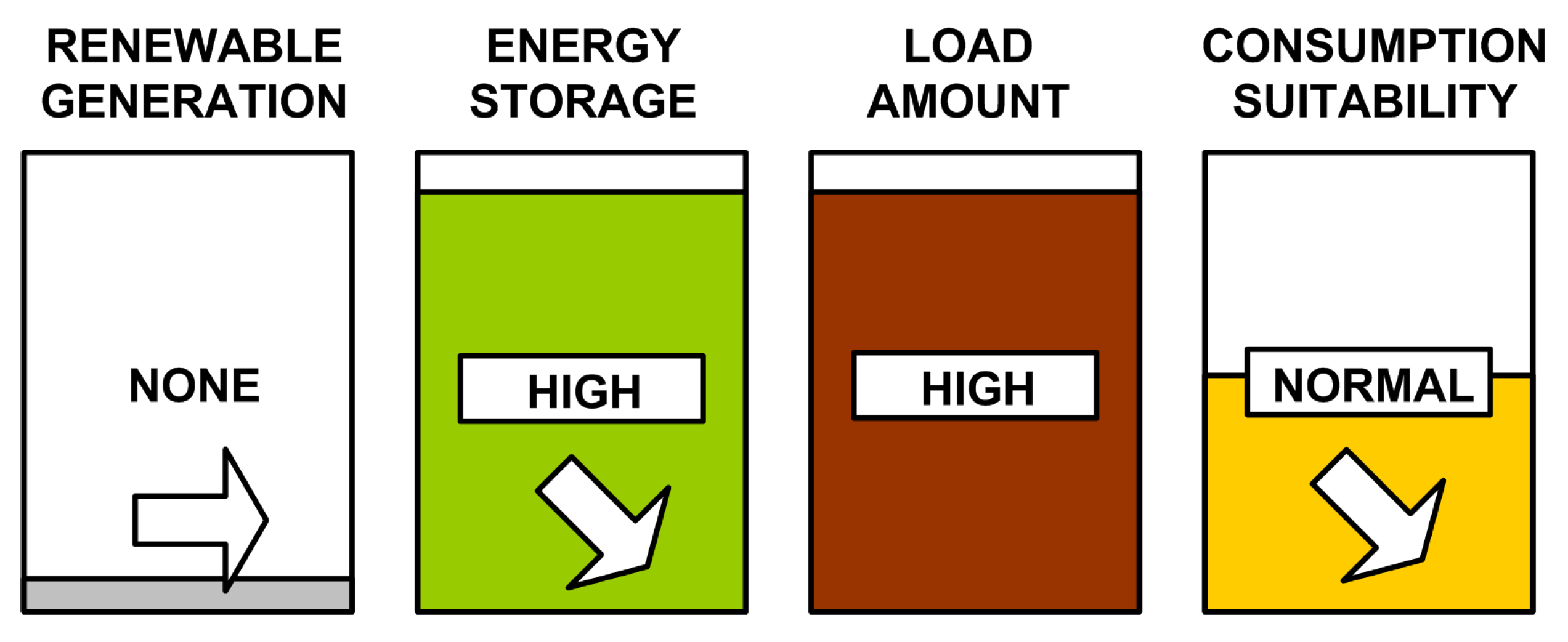
  The optimized running of a stand-alone HPS requires users’ awareness and collaboration. By means of GUIs or indicators lights adequately placed in the home environment, users can obtain useful system feedback in order to keep a correct and proactive behaviour. An intuitive, basic proposal of feedback panel for GUIs is shown in Figure 6. In the example, users get real-time meaningful information of the system status. They obtain estimations of the current level of renewable generation, the energy available in batteries, the load demand according to the system size and capacities and, finally, advice showing if consuming energy is appropriate or must be reduced (last indicator on the right side). Arrows add a dynamical, predictive dimension informing about the expected next status.

Figure 6. Example of system feedbacks addressed to users. Arrows mark predicted evolution or tendency.

Figure 6. Example of system feedbacks addressed to users. Arrows mark predicted evolution or tendency.

Due to the scenario dependence, algorithms that find optimized values for the introduced thresholds and related parameters are difficult to develop. So far, designs use rough but satisfactory values based on the practitioners experience and the design guidelines obtained from the related literature (e.g., [20,21]) and the specific battery documentation provided by manufacturers. GEINCO application, as a simulation tool, is expected to provide accurate parametrization for a given scenario. Also other common, publicly available simulation tools are being used for parameter optimization (e.g., TRNSYS).

5. DSM Test by Simulations

In order to check the suitability of some of the proposed DSM strategies, a set of simulations have been executed deploying the GEINCO application. Models and parameters have been selected as realistic as possible following the FSA system equipment features and using data collected from a stand-alone rural house actually connected to a FSA and owned by the Wattpic company (partially used as a test-bed environment).

5.1. Boundary Conditions & Component Models

For the simulations, data concerning PV generation have been obtained from a FSA of 2 kWp (single azimuthal axis and 45${}^{\circ }$ PV inclination, it is smaller compared with the current commercial models), collected from 10th to 20th April 2004 in la Llagostera (Catalonia, Spain), 41${}^{\circ }$49${}^{\prime }$ N 2${}^{\circ }$53${}^{\prime }$ E. The average power generation for the selected 10 days is 640 W.

The selected diesel engine has a maximum power of 7.5 kW with a maximum consumption rate of 3.4 L/h and 1 L/h at the minimum. As far as the battery group is concerned, it is formed by lead-acid tubular vented cells with $C_{20}=122$ Ah, arranged in 7 parallel branches of 11 cells per branch. The total capacity of the group is roughly $C_{10}=500$ Ah.

5.2. Electrical Loads

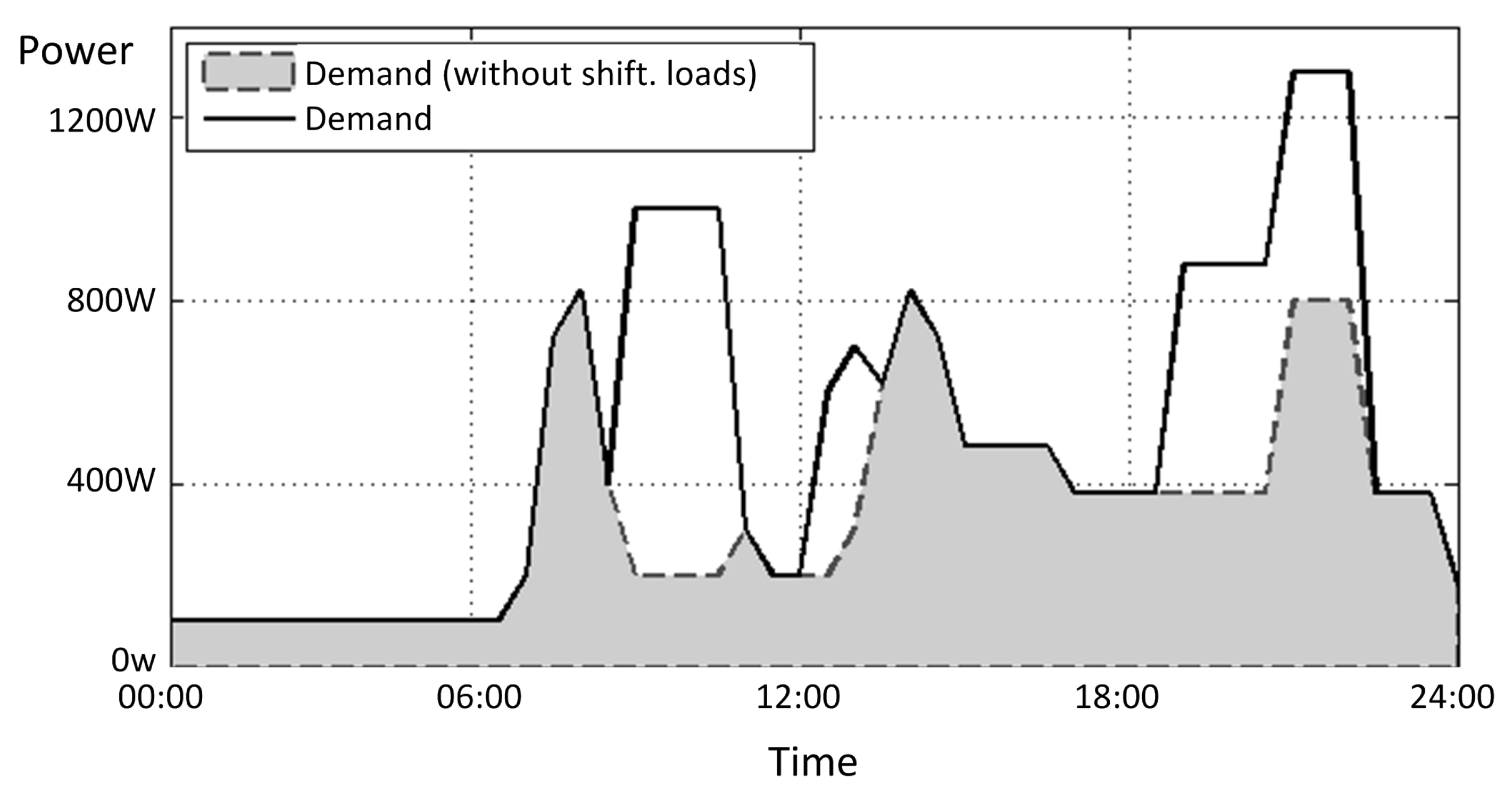
Electrical loads are designed according to the demand curves collected from the stand-alone house under test for a weekly scope. Figure 7 shows the representative, habitual load demand curve adapted to a daily scope. Note that shiftable loads are differentiated but still placed in their common supply period according to users’ behaviours and habits. In principle, the white areas in the figure are susceptible to be managed and moved by DSM strategies.

Figure 7. Representative demand curves from the stand-alone house model.

Figure 7. Representative demand curves from the stand-alone house model.

For the simulated period, the average power demanded by loads is roughly 495 W (shiftable loads included). From here, three shiftable loads have been modeled considering a daily basis:

• Watering pumps. Summarized as one daily divisible load of 800 W with a length of 2 h;
• Washing machine or dishwasher. Summarized as one daily shiftable load of 500 W with a length of 3.5 h;
• Supporting water heater. Summarized as one daily shiftable load of 400 W with a length of 1 h.

5.3. Compared Performances

Different tests have been carried out assuming diverse parametrization. For the selected scenario, we compare what is called a classic performance with an advance performance. They are defined as follows:

• Classic:
  –only C and
  –SocT with $t{h}_{SOC}=75\%$.
• Advanced:
  –SocT with $t{h}_{SOC}=75\%$.
  –LnT with $t{h}_{ld}=1.5$ kW.
  –BCSL, with the first threshold (suitable conditions) $t{h}_{SOC}^1=90\%$ and second threshold (excellent conditions) $t{h}_{SOC}^2=96\%$.
  –BCDL, with the first threshold (activation) $t{h}_{SOC}^A=92\%$ and second threshold (deferment) $t{h}_{SOC}^D=88\%$.

As far as the values of parameters are concerned, they have been established based on the next assumptions. In renewable energy installations with large number of batteries and where maintenance is expensive, energy systems are often sized to 20% to 50% depth of discharge (DOD) in order to reduce costs by lengthening battery life as much as possible [22]. The allowed DOD strongly depends in the specific type of batteries. Hence $t{h}_{SOC}$ in the selected example follows the usual configuration employed by Wattpic in their projects according to the equipment specifications and derived calculations. Similarly, high discharge rates are also controlled by $t{h}_{ld}$ according to battery manufacturers’ information. Finally, BCSL and BCDL thresholds are adjusted after diverse parameter sweep peformed by the GEINCO simulator.

6. Execution & Simulation Results

6.1. System Evolution

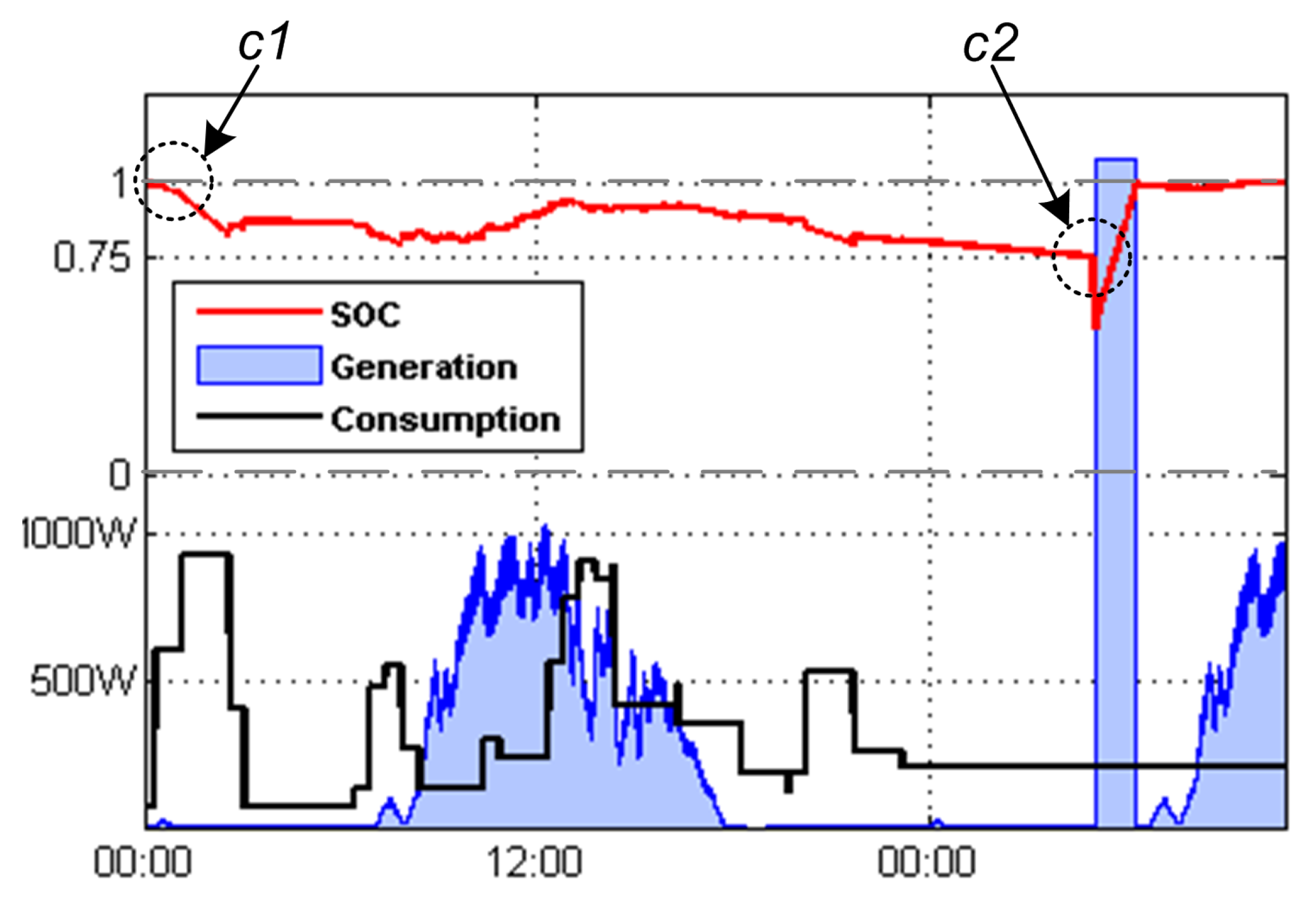
In order to have a better appraisal of the system running and evolution, Figure 8 shows superimposed, representative curves corresponding to an example day with low generation and considerable energy demand.

Since there are no forbidden time slots for shiftable loads, the system decides to supply some of them at midnight as batteries are fully charged (point c1). Shiftable loads feed on batteries in a time where there is no PV generation and some hours later cause a drop in the SOC level that momentarily stops the active divisible load. Afterwards, the system manages to supply the demand for the rest of the day, partially recovering thanks to the PV generation (about 50% lower than the expected in a sunny day). In any case, in the second half of the graphic the system is forced with a continuous demand of 300 W that ends up switching on the diesel generator to avoid that batteries drop under 75% of their capacity (point c2). The diesel generator satisfies the demand and also charges the batteries at their maximum level.

Figure 8. Example of day with low generation and considerable demand.

Figure 8. Example of day with low generation and considerable demand.

6.2. Comparison Results

After 10 days of simulation, we obtain results of both classic and advanced configurations. Table 2 summarizes the results with some performance indexes.

Table 2. Simulation Results.

Index/Variable	Classic	Advanced
days	10	10
SOC (start)	1	1
SOC (end)	0.89	0.87
Consumed energy	118.7 kWh	116.6 kWh
Supplied by batteries	2.4 kWh	2.4 kWh
Supplied by diesel	35.7 kWh	26.5 kWh
Supplied by PV	80.6 kWh	87.7 kWh
Peak-sun hours/day 1	5.4 h	5.8 h
Non diesel generated 2	69.9%	77.3%
Consumed fuel	19.73 L	14.12 L
kWh/L	1.81	1.88
diesel efficiency	82.2%	85.1%

Notes: ¹ It is a calculation based on the PV generation. The higher value of the advanced strategy means that it is more efficient making the most of the sun energy. The yearly average calculated by [23] for the same region and considering 45${}^{\circ }$ inclination is 3.7 peak-sun hours per day; ² Percentage of energy that does not virtually come from the diesel generator during simulations. It is supplied by the PVs (sometimes through batteries) plus a little amount of energy taken from the initial charge of batteries (the origin of this initial store is a priori unknown).

Table 2. Simulation Results.

Index/Variable	Classic	Advanced
days	10	10
SOC (start)	1	1
SOC (end)	0.89	0.87
Consumed energy	118.7 kWh	116.6 kWh
Supplied by batteries	2.4 kWh	2.4 kWh
Supplied by diesel	35.7 kWh	26.5 kWh
Supplied by PV	80.6 kWh	87.7 kWh
Peak-sun hours/day 1	5.4 h	5.8 h
Non diesel generated 2	69.9%	77.3%
Consumed fuel	19.73 L	14.12 L
kWh/L	1.81	1.88
diesel efficiency	82.2%	85.1%

Notes: ¹ It is a calculation based on the PV generation. The higher value of the advanced strategy means that it is more efficient making the most of the sun energy. The yearly average calculated by [23] for the same region and considering 45${}^{\circ }$ inclination is 3.7 peak-sun hours per day; ² Percentage of energy that does not virtually come from the diesel generator during simulations. It is supplied by the PVs (sometimes through batteries) plus a little amount of energy taken from the initial charge of batteries (the origin of this initial store is a priori unknown).

The existing differences in the consumed energy between both cases (1.8%) are due to the fact that battery charging and discharging show an implicit coefficient of performance about 0.8. Since the relationship between generation and demand is improved, energy leaving and returning to the batteries happen at a lower rate, hence lower consumption is required to accomplish the same work.

The exploitation of PV energy improves (8.9%) on account of the fact that periods where batteries are full and PV are generating energy result minimized. DSM strategies cause this effect as they relocate shiftable loads in the most profitable moments. In addition, a little part of such difference is due to the fact that, whenever the diesel generator is switched on, in that moment PV generation is wasted. In other words, reducing the usage of the diesel source entails the reduction of losses as simultaneities are avoided. Note that fuel savings account for about 28%.

Moreover, the system has a better control of the diesel source start and stop. It has an impact on the amount of load that is set for the expected diesel supply, making the engine to run in higher power rates. As a result, the diesel source performance is also enhanced.

7. Discussion

The test conducted in the previous section highlights that important savings can be achieved by sound DSM strategies adapted or aware of the HPS system nature. Noteworthy, the shown results are illustrative, but do not try to offer a representative measure of savings achieved by the application of DSM strategies. Other scenarios have been simulated and tested with lower distances in the levels of consumed fuels, but note that not all the presented DSM strategies are applied either. Informative and persuasive strategies for energy savings are difficult to be tested by simulations; but point to be productive [5], specially marked for DG and HPG, which are more delicate solutions than classical central grids and where users aware of the particular system dynamics is a key factor for the system efficiency.

In general terms, the impossibility to give precise rates of potential savings are due to the fact that the final effect and behaviour of DSM strategies show a high dependence on the specific scenario. For example, stable consumption habits and a set of movable-defined loads draw situations where the control system has more freedom and capabilities to make the most of the available energy sources and storage units. In short, the presented DSM strategies precisely intend to confer flexibility and adaptability to the whole system in an application field where optimization and exhaustive exploitation of resources are mandatory.

8. Conclusions

This paper has shown (a) a set of DSM strategies adaptable to stand-alone HPS; (b) an overview of the requirements in terms of network, hardware and software to implement DSM in a real HPS case; and (c) a simulated performance comparison that supports the expectation of benefits to be obtained by the application of some of the proposed DSM strategies. Thus, the suitability of the introduced DSM strategies for a HPS provided with a consistent underlying system is confirmed. Now, next steps can be considered taking into account the two displayed perspectives:

On one hand, DSM strategies must be dealt together with PMS to reach optimization and synergistic performances. Furthermore, the refining of parameters and strategies is expected as a result of sensitivity analysis carried out using common simulation tools (e.g., TRANSYS, PVsyst), but also by means of the GEINCO application, which entails further advantages as it allows a closer and more tailored description of the specific case, installed equipment, supplied loads and implemented strategies. Additional renewable sources (e.g., wind) and components (e.g., fuel cells) for the design and refinement of DSM are also to be considered.

On the other hand, with regard to the presented HPS framework, enhancements in both networks (data acquisition and load control) are planned. New developments entail hardware and software developments, allowing plug and play connection of endpoint devices and improved control features. It is mandatory to ameliorate communication capabilities and allow the integration with other common automation protocols (mainly wireless). Finally, the maturing of the control application requires the constant development of libraries with alternative and more accurate models, strategies, algorithms and components.