Non-Intrusive Demand Monitoring and Load Identification for Energy Management Systems Based on Transient Feature Analyses

Abstract

Energy management systems strive to use energy resources efficiently, save energy, and reduce carbon output. This study proposes transient feature analyses of the transient response time and transient energy on the power signatures of non-intrusive demand monitoring and load identification to detect the power demand and load operation. This study uses the wavelet transform (WT) of the time-frequency domain to analyze and detect the transient physical behavior of loads during the load identification. The experimental results show the transient response time and transient energy are better than the steady-state features to improve the recognition accuracy and reduces computation requirements in non-intrusive load monitoring (NILM) systems. The discrete wavelet transform (DWT) is more suitable than short-time Fourier transform (STFT) for transient load analyses.

1. Introduction

The traditional method of load monitoring is based on supervisory control and data acquisition (SCADA). Sensors are installed at every load, and a communication network is required for monitoring, communication, and control. Once the load recorder receives a sensor message, it immediately records the load data and delivers them to the data center for further analyses. However, the traditional load monitoring method is too complicated to implement in an ordinary household [1].

Schweppe and Hart proposed non-intrusive load monitoring (NILM) [2]. An NILM system does not require a voltage or current sensor at every load, and it determines the operating schedule of the major electric loads in a building at the power service entrance. Compared with the traditional load monitoring system, NILM systems offer simple hardware installation. Therefore, an NILM system is a wide load monitoring scheme and a powerful energy management system [3,4,5,6]. Figure 1 shows the overall scheme of an NILM system. Three-phase or one-phase electricity powers the loads, which are representative of important load classes in a residence. A meter data management system (MDMS) connects to the NILM system to manage and measure the operation, load quality, and power demand of each load using a wire or wireless sensor network. The client computers can also read all the information from the MDMS through the Internet or Web systems.

Figure 1. Data collection and load identification system for an NILM system.

Figure 1. Data collection and load identification system for an NILM system.

Hart proposed a load identification method that monitors the steady-state behavior of loads. Hart conceptualized a finite state machine to represent a single appliance in which power consumption varies discretely with each step change. Although this method performs well, it has some limitations. For example, this method cannot monitor small appliances or appliances that are always on or have non-discrete changes in power [2,5]. Cole [7,8] presented a data extraction method and a steady-state load identification algorithm for NILM. The algorithm developed by Cole can be used for load switching between individual appliances when one or more appliances are switched on or off. However, this algorithm requires an extended period of time to accumulate real power (P) and reactive power (Q) data, and cannot recognize any appliance power consumption that does not change [8].

Several recent studies have proposed new power signature analyses [9,10,11] and load identification methods [12,13,14,15] to recognize loads and to solve classification problems. In 2005, Lee presented an estimation technique using unique harmonic signatures to monitor variable-speed-drive (VSD) power consumption in a NILM system. Furthermore, to indicate the time-varying nature of VSD power demand makes it difficult to keep the track of the ON/OFF status of other constant loads [10]. Many load identification papers aiming to improve recognition performance using artificial neural networks (ANNs) for an NILM system have been published. For example, Srinivasan et al. [14] proposed a neural-network-based approach to identify non-intrusive harmonic sources. Their method does not incorporate the various operational modes of each load and operation under different voltage sources. Practical power systems contain many harmonics. Previous research has demonstrated how harmonics affect the results of an NILM system [16]. However, harmonic content for constant linear loads is very small [10], therefore, features other than harmonics and steady-state signatures are necessary for load identification in commercial buildings and residential customers.

To mitigate the disadvantages of steady-state signatures in previous research, this study proposes a new analysis method for load identification in an NILM system. This method uses the transient energy signature (U_T) and transient response time (t_TR) to improve the recognition accuracy and reduce computational requirements. The proposed improvement technique is unrelated to operational mode, voltage variations, and power consumption change. This proposed method is suitable for different loads with the same real and reactive power or with simultaneous starting times. Experimental results show that the proposed method for the NILM system achieves efficient recognition of commercial or industrial loads and improves computational requirements.

This paper is organized as follows: the proposed methods such as the calculation of transient response time of WT and transient energy of power features are described in Section 2. The effects of transient power features and feature analysis for load identification are addressed in Section 3. Based on the feature analysis techniques, t_TR and U_T, and the load recognition method, and a series of experiments such as software simulation and measurement on site are analyzed and discussed in Section 4 to prove the feasibility of the method proposed in this paper.

2. Proposed Methods

The traditional non-intrusive load monitoring system uses P and Q as power signatures. However, false identification occurs when the power of a certain load equals the total power of the other loads in the NILM system [1]. To counteract this problem, this method uses turn-on/off transient waveforms to identify loads and analyze their characteristics.

2.1. Transient Response Time

Morlet and Grossman proposed the concept of WT to overcome the problems of the STFT, such as difficult choice of window functions and proper range of frequency [17]:

$${\psi }_{a,b}(t)=\left|\frac{1}{\sqrt{a}}\right|g(\frac{t-b}{a})$$

(1)

where ${\psi }_{a,b}(t)$ is called the daughter wavelet and $g(\frac{t-b}{a})$ is the dilated and translated mother wavelet. Parameter a is the scale factor, and b is the shift factor. The wavelet transform essentially uses scale and shift factors to decompose the signal being analyzed into a series of mother wavelets. Therefore, it is better suited to analyze transients [18]. A wavelet transform includes the continuous wavelet transform (CWT) and DWT. CWT is defined as:

$$CW{T}_{a,b}={\displaystyle {\int }_{-\infty }^{\infty }x(t){\psi }_{a,b}^{\ast }(t)dt}$$

(2)

where x(t) is the original signal. To obtain the DWT, it is necessary to discretize the scale factor and shift factor:

$$a=a_0^m;b=n{b}_0{a}_0^m$$

(3)

Substituting Equation (3) into Equation (2) leads to Equation (4):

$$DW{T}_{m,n}={\displaystyle {\int }_{-\infty }^{\infty }x(t)\left|a_0^{-\frac{m}{2}}\right|}{g}^{\ast }(\frac{t-n{b}_0{a}_o^m}{a_0^m})dt=a_0^{-\frac{m}{2}}{\displaystyle \sum _{k}x[k]g[a_0^{-m}}k-n{b}_0]$$

(4)

Setting:

$$a_0=2;b_0=1$$

(5)

the result becomes:

$$DW{T}_{m,n}==2^{-\frac{m}{2}}{\displaystyle \sum _{k}x[k]g[2^{-m}}k-n]$$

(6)

The DWT decomposes the original signal into detailed and approximate signals using high-pass filter (h[n]) and low-pass filter (g[n]), respectively. The DWT algorithm of multi-resolution decomposition is illustrated in Figure 2. Equation (7) shows the relationship between high-pass and low-pass filters. Daubechies wavelets are widely used to solve a broad range of problems (e.g., self-similarity properties of a signal or fractal problems, signal discontinuities, noise suppressions).

$$h[L-1-n]={(-1)}^{n}g[n]$$

(7)

Figure 2. Discrete wavelet transform scheme.

Figure 2. Discrete wavelet transform scheme.

Steady-state signatures, such as P and Q, are additive when two loads occur simultaneously. The power of an unknown load can equal that of other composite electrical loads when these loads exist simultaneously. Thus, it is not possible to identify the unknown load from these composite electrical loads based only on the real power. In addition, the values of these steady-state signatures change when electric equipment is used for a long time because operation temperature (e.g., hair dryers and vacuum cleaners). Figure 3 shows the real power of a 1200 W vacuum cleaner operating for approximately 6 min. In contrast to steady-state properties, transient properties are not additive [3] and are unaffected by operation temperature.

Figure 3. Real power waveform of a 1200 W vacuum cleaner.

Figure 3. Real power waveform of a 1200 W vacuum cleaner.

Transient response time is related to the time constant of the physical properties of load. The time constant directly results from the resistance, inductance, and capacitance of electric load. These parameters change with the operation temperature, and therefore influence the physical behavior of load and some power signatures (e.g., P, Q, and harmonics) if the electric load is used for a long time. Conversely, these parameters do not affect the recognized pattern for an extremely short time such as a transient state.

Equation (8) shows the transient response time, t_TR. The following sections discuss and describe the detection of transient ending time and starting time of the discrete wavelet transform (DWT) and short-time Fourier transform (STFT):

$$t_{TR}=t_{end}-t_{start}$$

(8)

where t_end is a derivative of transient ending time from STFT or DWT, and t_start is detected by the transient starting time of the STFT or DWT.

The starting time can be searched for using the maximum value in the scale 1 details (d1) of DWT and the first non-steady state frequency band of STFT, respectively. The ending time can be found using the maximum value in the scale 5 details (d5) of DWT and the first steady state frequency band of STFT, respectively.

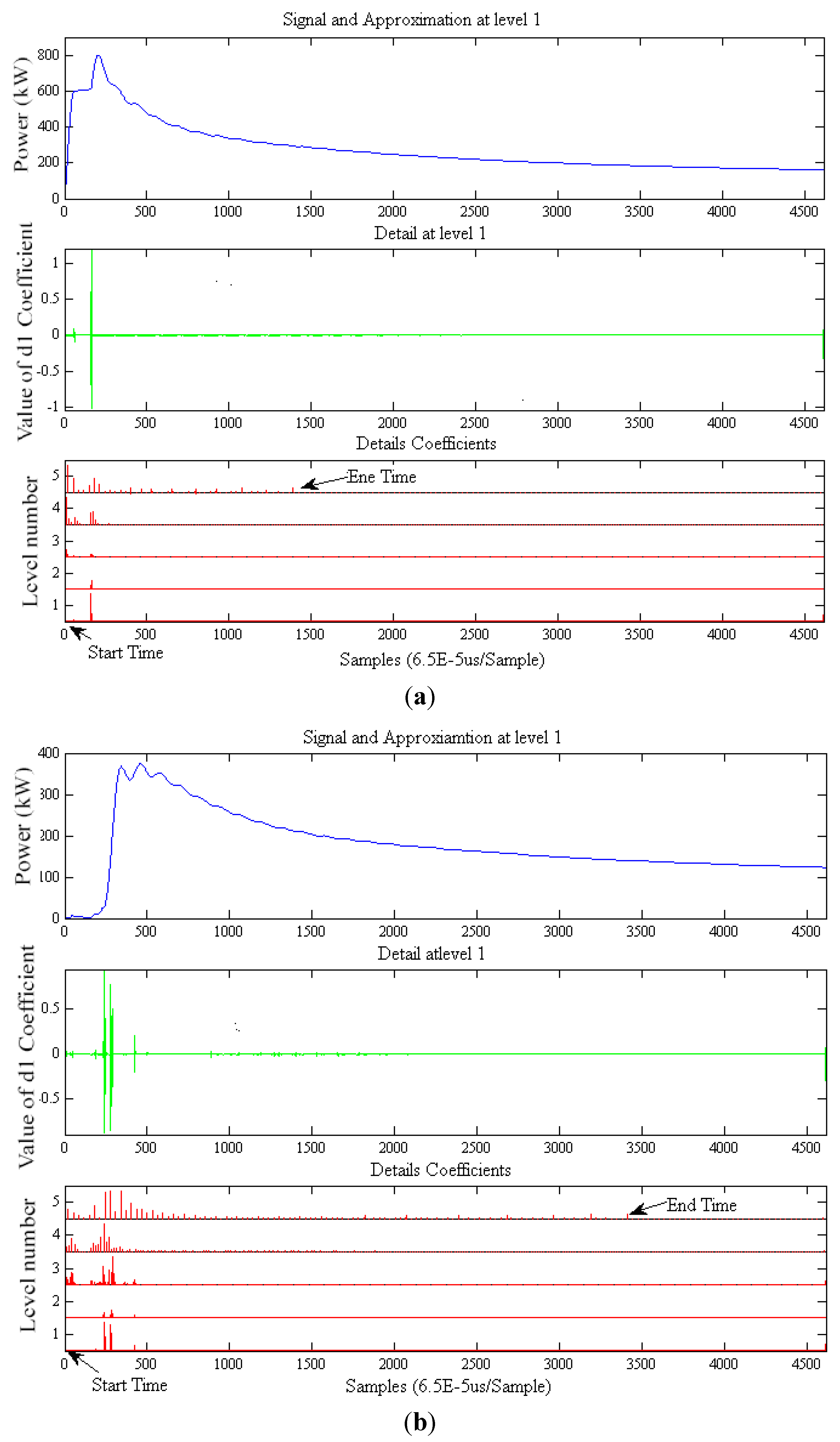
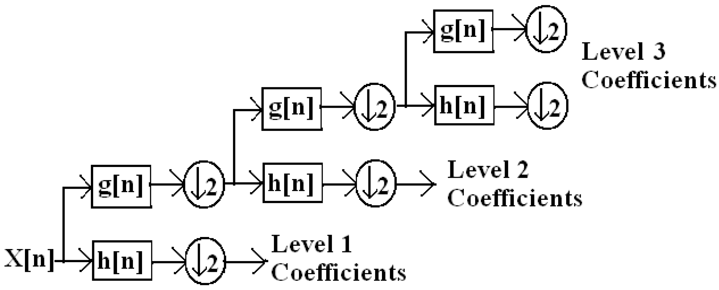
2.2. Transient Energy Algorithms

The transient properties of a typical electrical load are primarily determined by the physical task that the load performs [19,20]. For example, estimating current waveform envelopes at the utility service entrance of a building allows accurate transient event detection using NILM [19]. Therefore, load classes performing different tasks can be distinguished by their transient behavior [19,20]. Because the envelopes of turn-on/off instantaneous transient power are closely linked to unique physical quantities, they can serve as reliable metrics for load identification. However, the transient state is the dominant state directly after load inception. The one-phase transient energy can be determined as follows:

$$V(k)=v(k)-v(k-1)$$

(9)

$$I(k)=\frac{(i(k)+i(k-1))}{2}$$

(10)

$$U_T=U_{1\varphi ,transient}={\displaystyle \sum _{k=0}^{K}V(k)I(k)}$$

(11)

where V(k) is derived from the transient voltage for sample k, I(k) is average transient current for sample k, v(k) is voltage sampled for sample k, v(k − 1) is voltage sampled for sample k − 1, i(k) is current sampled for sample k, i(k − 1) is current Sampled for sample k − 1, and K is number of samples, k = 1, 2,…,K.

The three-phase transient energy can be computed as follows:

$$U_T=U_{3\varphi ,transient}={\displaystyle \sum _{k=0}^K\left(Va(k)\cdot Ia(k)+Vb(k)\cdot Ib(k)+Vc(k)\cdot Ic(k)\right)}$$

(12)

where $V_a(k),V_b(k),V_c(k)$ are derivatives of transient voltage in phases a, b, and c for sample k; $I_a(k),I_b(k),I_c(k)$ are the average value of transient current in phases a, b, and c for sample k.

2.3. Multi-Layer Feedforward Neural Network

A backward error-propagation algorithm updates interconnecting weights and thresholds until it attains proper recognition capability. The back-propagation classifier (BP) in this study is generally used as a trainable classifier for a multi-layer feedforward neural network (MFNN). “Classification” in this context denotes a mapping from a feature space to the set of class labels—the names of commercial or industrial load combinations.

Bayesian regularization (mean square error, MSE) typically provides better generalization performance than early stopping because Bayesian regularization does not require a validation dataset to be separated from the training dataset. On the other words, the input training data uses all training datasets. This advantage is particularly important when the dataset is small.

A supervised MFNN generally consists of three layers: input, hidden, and output, including neurons. The neurons are connected by links with weights that are selected to meet the desired associations between the input and output neurons. These weights must be trained with existing input-output pairs using an appropriate algorithm. The purpose of the MFNN in this study is to identify the load of an NILM system. This study adopts an MFNN based on the back-propagation method and this ANN can identify the similarities between given data and known data [21]. The input, output, and hidden layers of the ANN are described as follows:

(1)

Input Layer: The number of input neurons is the same as that of the power signature information, including the real and reactive power (PQ), PQ and total harmonic distortion of the voltage and current (PQV_THDI_THD), or transient response time and the transient energy signature (t_TRU_T) for comparisons. These power signatures are taken as input data from an electrical service entrance.

(2)

Output Layer: The number of output neurons is the same as that of the identified individual appliances. Each binary bit serves as a load indicator for the turn-ON/OFF status.

(3)

Hidden Layer: The proposed method uses only one hidden layer. Researchers have proposed various heuristic approaches to determine the number of neurons in the hidden layer [22]. The common number of neurons for the hidden layer is (number of input neurons + number of output neurons)/2 or (number of input neurons + number of output neurons)^0.5. Simulation results show no significant difference between these two options.

3. Transient Analyses

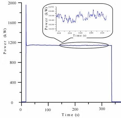
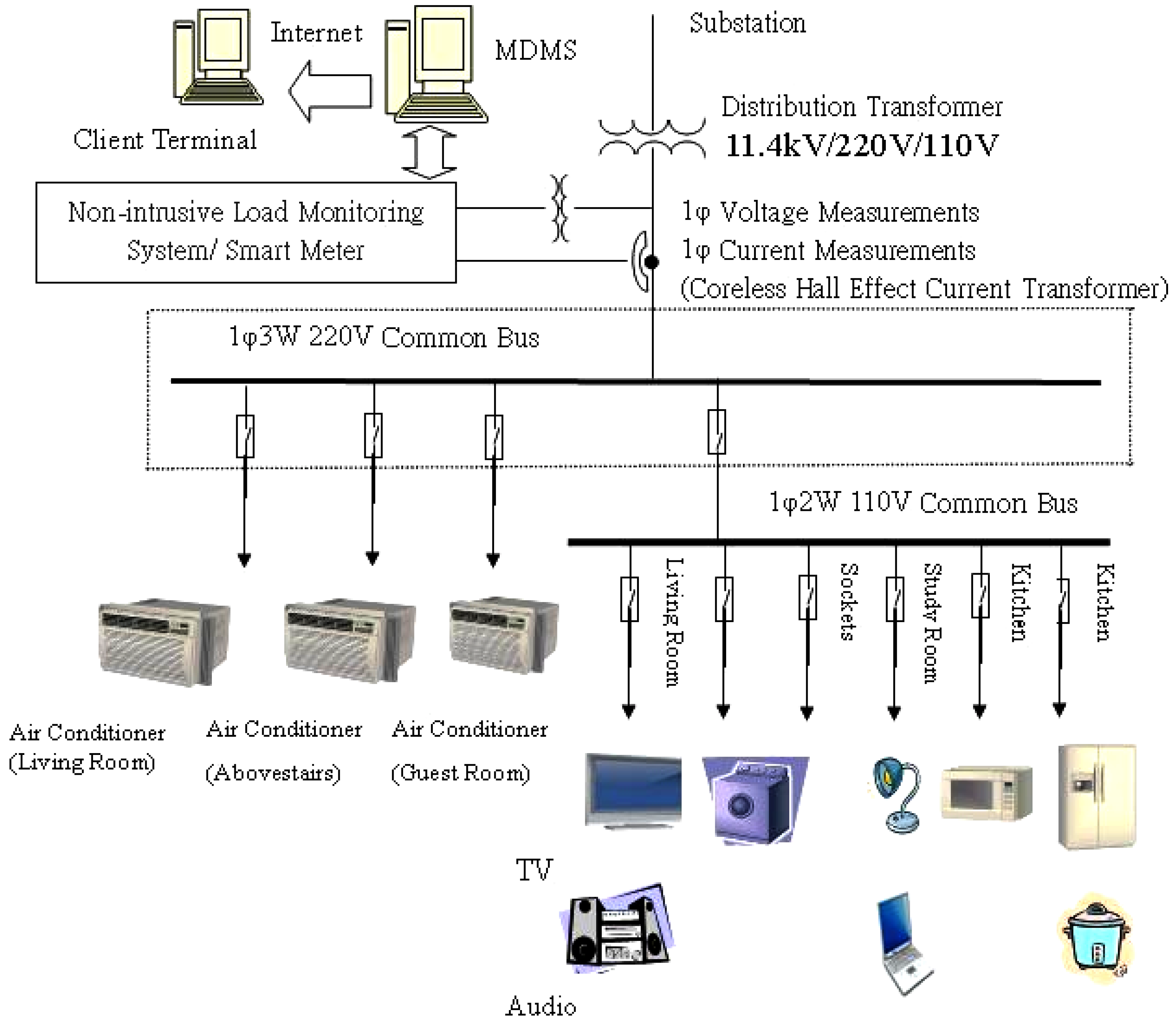
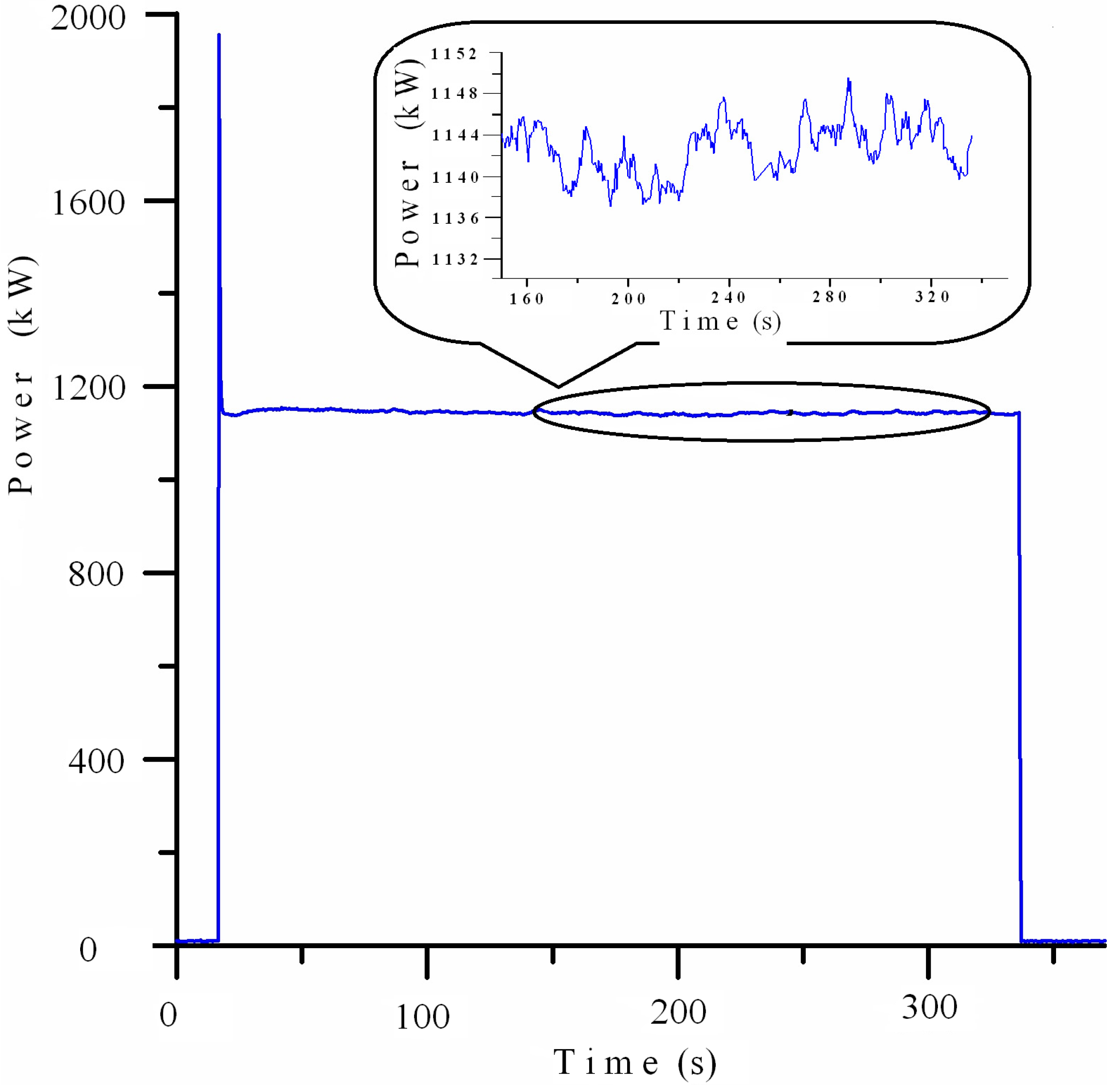
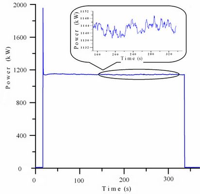
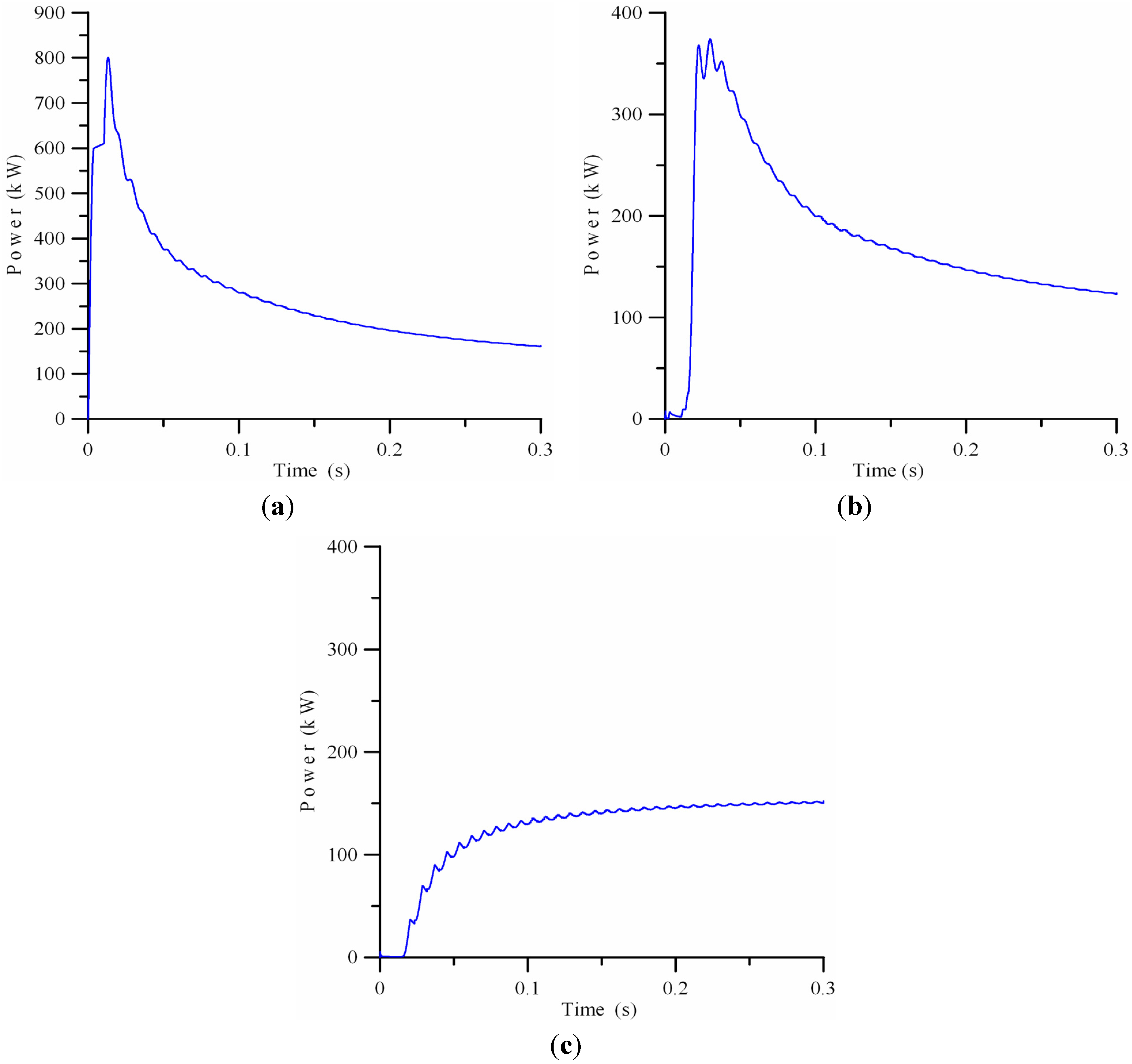
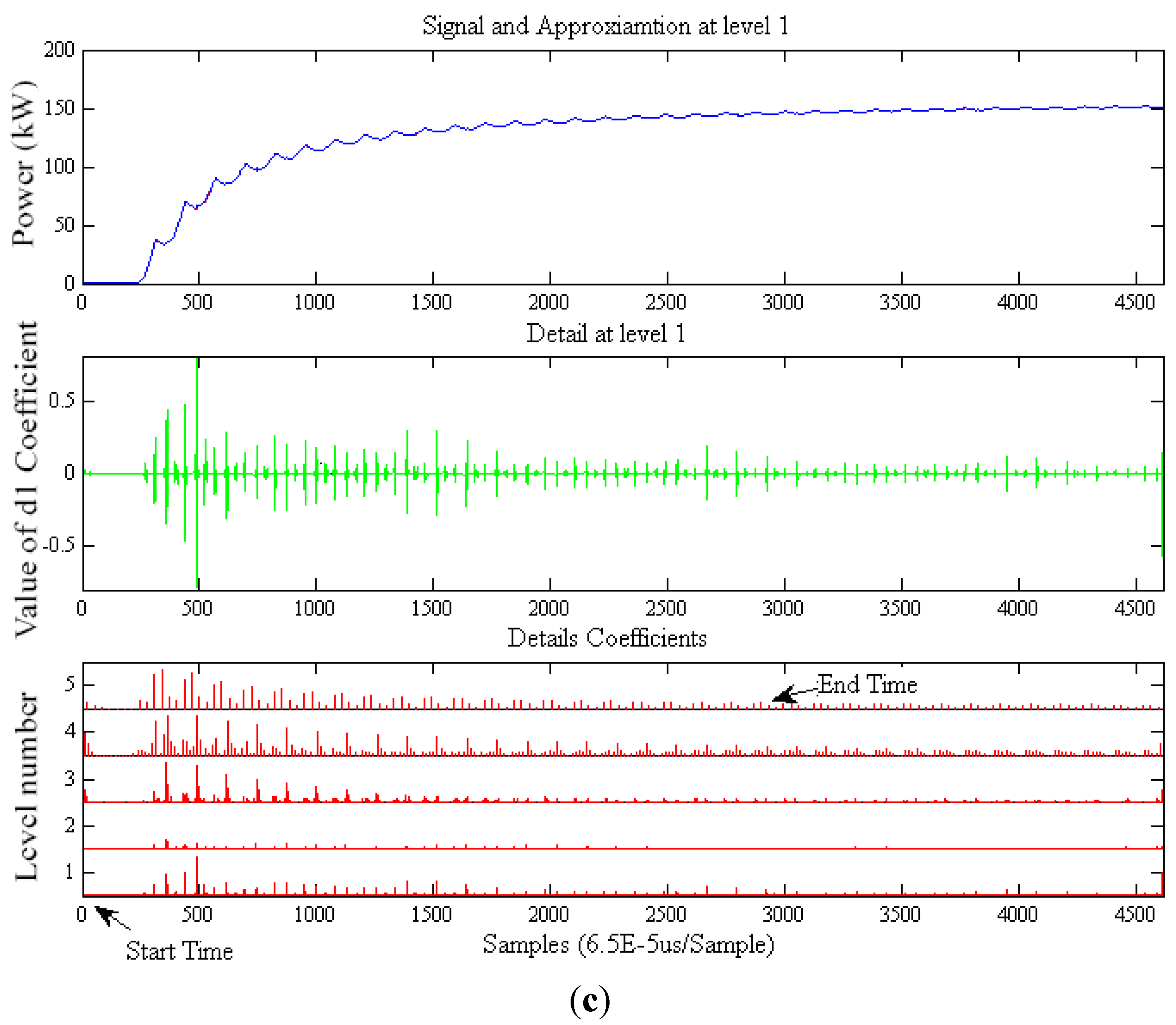
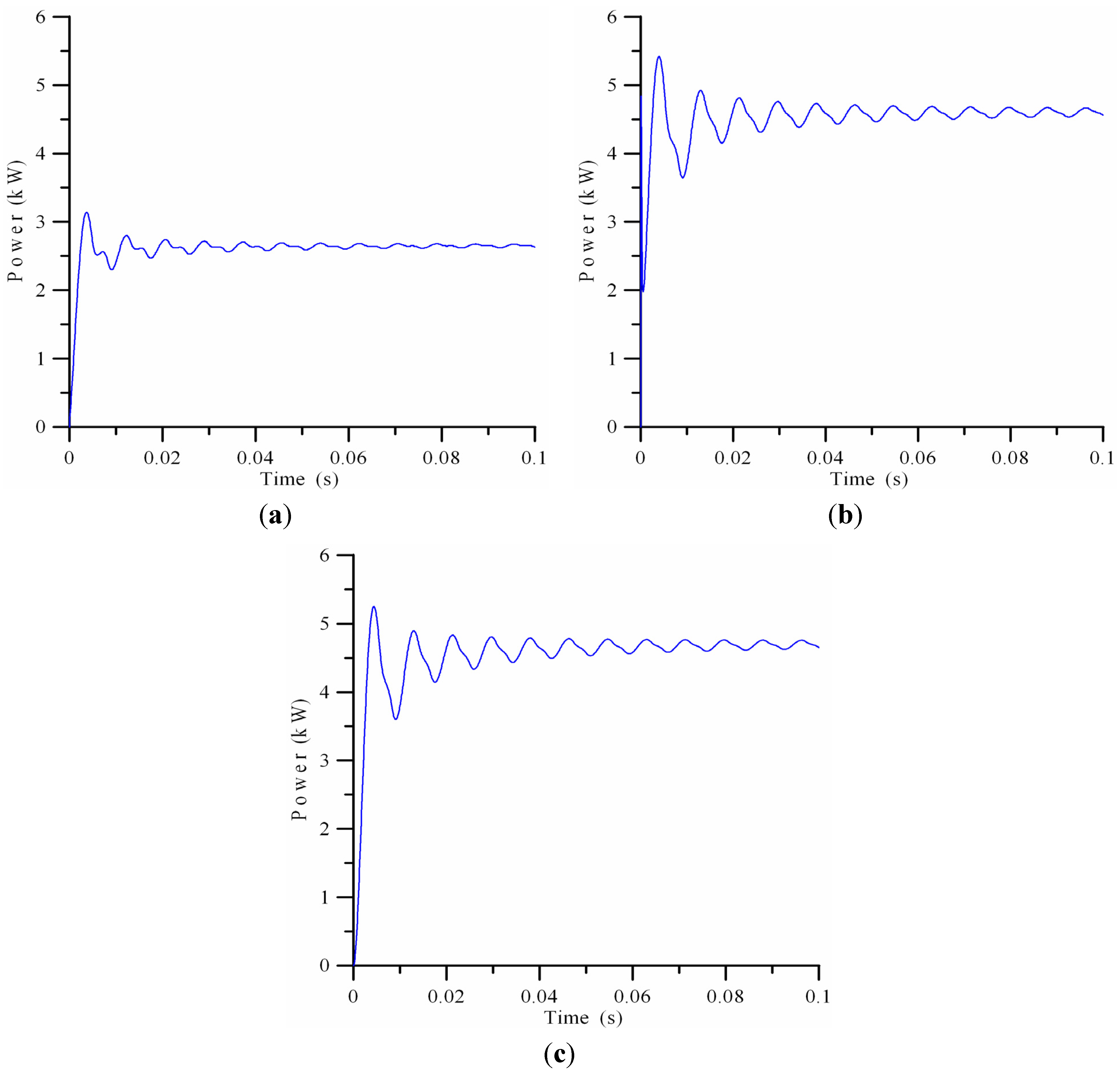
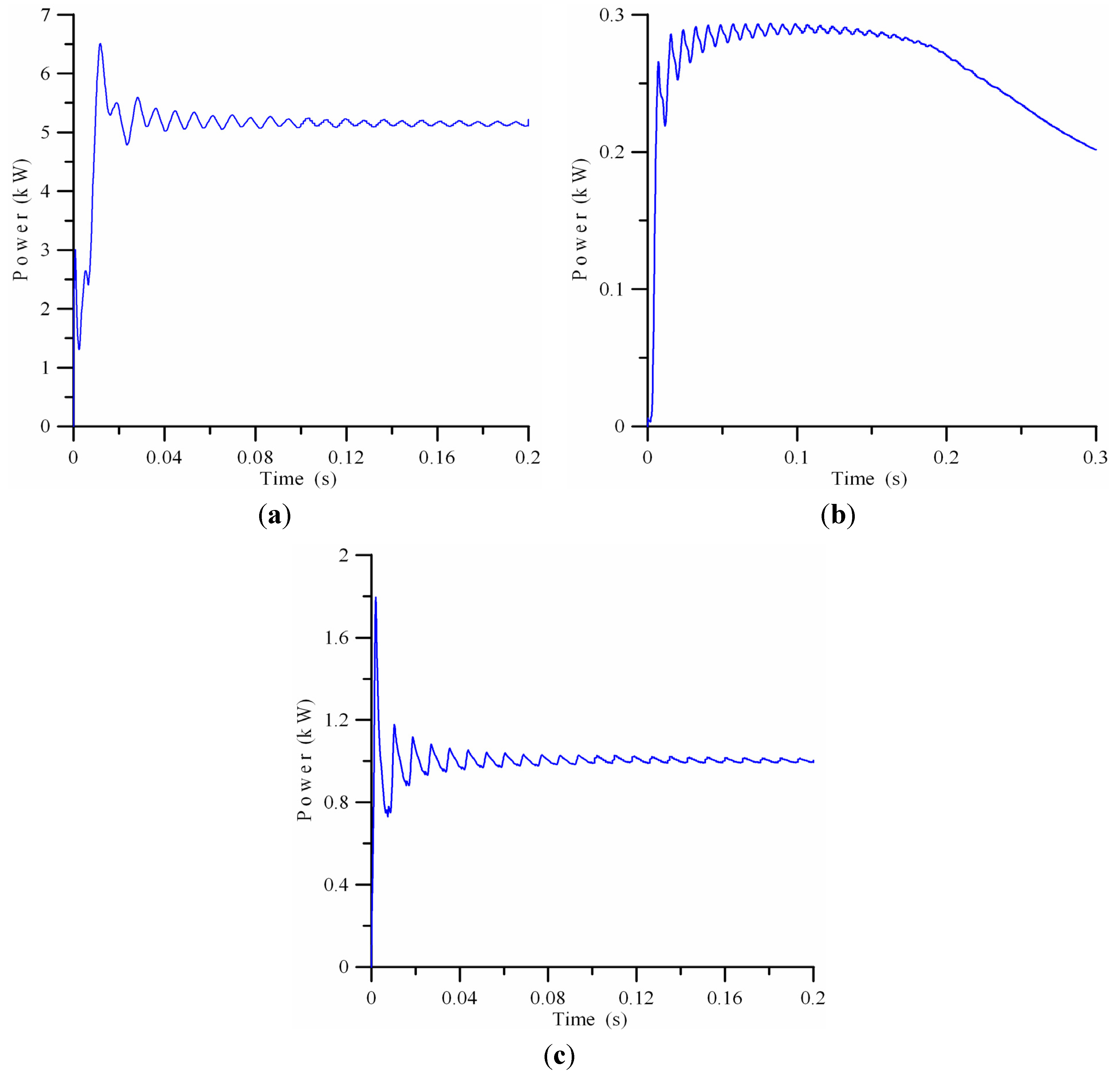
3.1. Data Acquisition and Measurement

The primary data in an NILM system are the voltage and current of aggregate loads from the point of common coupling (PCC) at the utility service entrance. The turn-on/off transients of the load were simulated by the Electromagnetic Transient Program (EMTP), and the data of the turn-on/off transients of the experimental load were measured on site using a Tektronix digital phosphor oscilloscope. The time duration for retrieving transient power signatures depends on different sampling frequency for NILM. This study adopts a 4 s time duration. A sample of 521 data samples for each cycle is sufficient, and therefore, the sampling frequency is approximately 30 kHz. A representative sample of the loads should be monitored to compile data for training purposes. The results of the STFT and DWT, along with the recognition of NILM system, were calculated using the MATLAB program. The program was run on a DELL PC equipped with an Intel 2.33 GHz Core 2 Duo CPU.

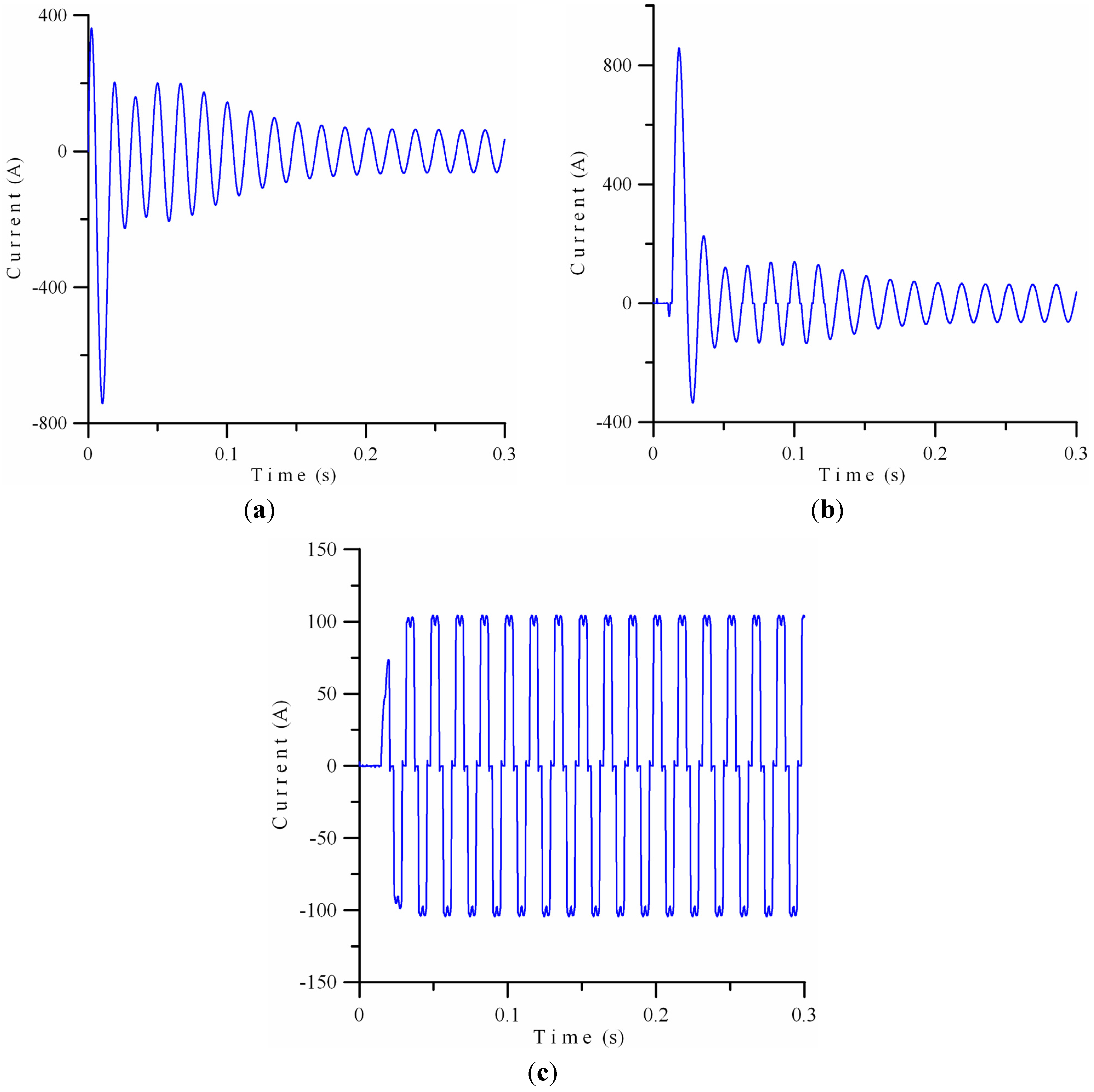
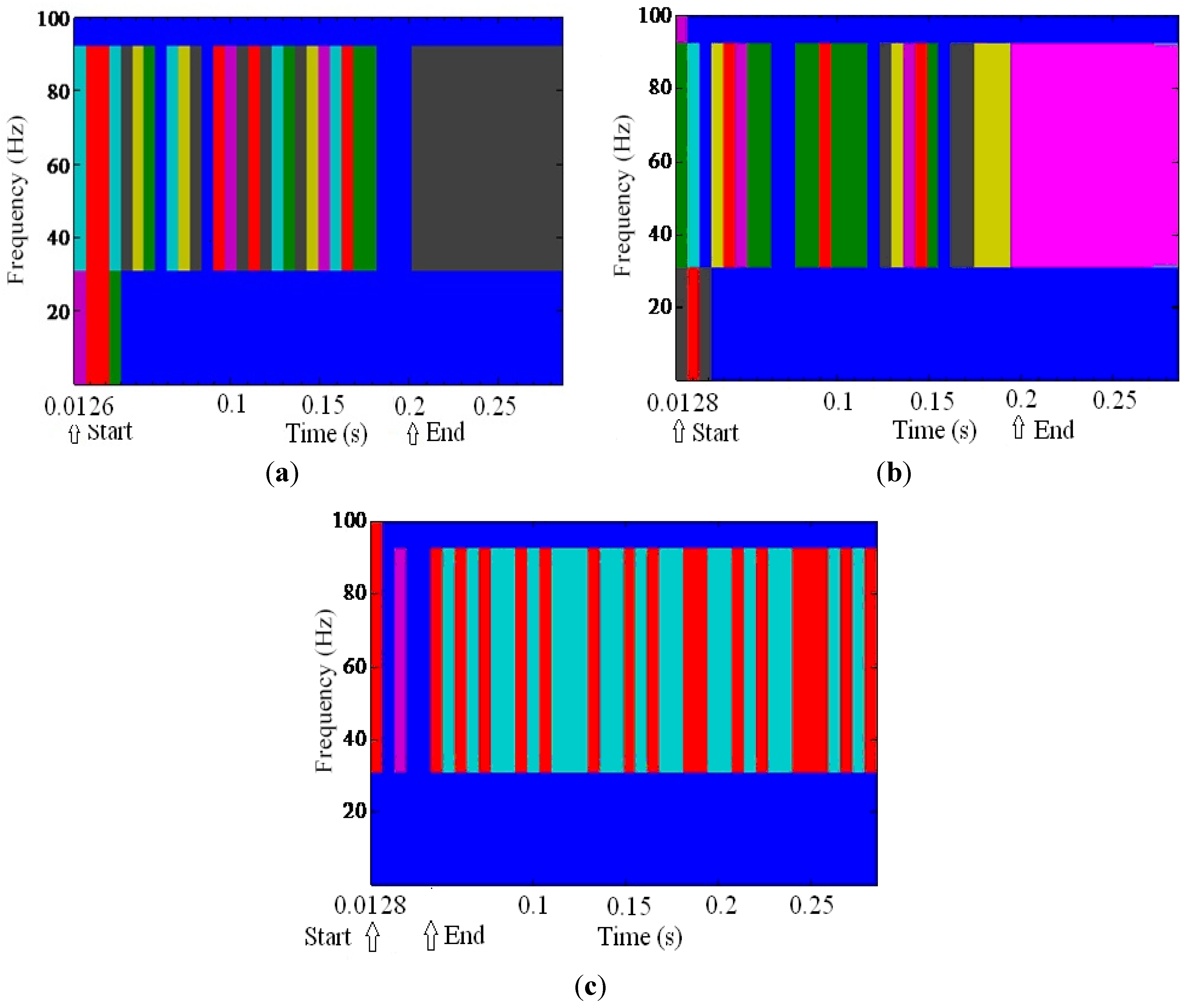
3.2. Analysis and Comparison

This study compares and analyzes the results of the STFT and DWT of the turn-on transients of three loads. Figure 4a–c show the current waveforms of turn-on transients for a 160 hp induction motor, a 123 hp induction motor driven by variable-voltage drives, and a bank of loads supplied by a six-pulse thyristor rectifier for AC power, respectively. Figure 5a–c show the results of the STFT for the turn-on current transients of the same loads in Figure 4a–c, respectively.

Figure 4. The current waveforms of turn-on transients. (a) a 160 hp induction motor; (b) a 123 hp induction motor driven by variable-voltage drives; (c) a bank of loads supplied by a six-pulse thyristor rectifier for AC power.

Figure 4. The current waveforms of turn-on transients. (a) a 160 hp induction motor; (b) a 123 hp induction motor driven by variable-voltage drives; (c) a bank of loads supplied by a six-pulse thyristor rectifier for AC power.

Figure 5. The STFT results of turn-on current transients. (a) a 160-hp induction motor; (b) a 123-hp induction motor driven by variable-voltage drives; (c) a bank of loads supplied by a six-pulse thyristor rectifier for AC power.

Figure 5. The STFT results of turn-on current transients. (a) a 160-hp induction motor; (b) a 123-hp induction motor driven by variable-voltage drives; (c) a bank of loads supplied by a six-pulse thyristor rectifier for AC power.

Figure 6a–c show the instantaneous transient power waveforms of turn-on transients for the same loads in Figure 4a–c, respectively. Figure 7a–c show the results of the DWT for the turn-on instantaneous transient power of the same loads in Figure 4a–c, respectively.

The turn-on transient waveforms clearly show the physical behaviors of the three electrical loads regardless of the current or instantaneous transient power waveforms. Comparing the turn-on transient waveforms with the steady-state waveforms for the same load indicates that the turn-on transient waveforms provide more physical characteristics than the steady-state waveforms. Figure 6a,b are different from turn-on instantaneous transient power waveforms because their start-up methods are different from each other. In Figure 6c, the instantaneous transient power waveform of the load slowly increases to the rated power because of the control method of the thyristor rectifier.

Figure 5 and Figure 7 show the STFT and DWT results for turn-on transients, respectively. The transient response time of each load can be identified from the ending time and the starting time. For the STFT results, the starting times are 0.0126 s, 0.0128 s, and 0.0128 s in Figure 5a–c, respectively. The ending times in Figure 5a–c are 0.2, 0.2, and 0.03 s, respectively. The starting times shown in Figure 4a–c are 0 s. However, the STFT uses a fixed window frame that cannot accurately identify the time. Moreover, any window function is subject to a certain degree of leakage.

In the results of DWT, the starting times in Figure 7a–c are 0 s. The ending times in Figure 7a–c are 0.1 s, 0.23 s, and 0.18 s, respectively. The starting time can be searched for using the maximum value in the scale 1 details (d1) of DWT, and the ending time can be found using the maximum value in the scale 5 details (d5) of DWT. This study uses Daubechies as the mother wavelet for WT. The event detection method uses the Daub4 WT of the envelope of instantaneous transient power waveform. Wavelet transform uses the scale factor and shift factor to resolve the original signal into approximation and details. Therefore, the wavelet transform results are better than those of the STFT.

Figure 6. The instantaneous power waveforms of turn-on transients. (a) a 160 hp induction motor; (b) a 123 hp induction motor driven by variable-voltage drives; (c) a bank of loads supplied by a six-pulse thyristor rectifier for AC power.

Figure 6. The instantaneous power waveforms of turn-on transients. (a) a 160 hp induction motor; (b) a 123 hp induction motor driven by variable-voltage drives; (c) a bank of loads supplied by a six-pulse thyristor rectifier for AC power.

Figure 7. The DWT results of turn-on instantaneous power transients. (a) a 160 hp induction motor; (b) a 123 hp induction motor driven by variable-voltage drives; (c) a bank of loads supplied by a six-pulse thyristor rectifier for AC power.

Figure 7. The DWT results of turn-on instantaneous power transients. (a) a 160 hp induction motor; (b) a 123 hp induction motor driven by variable-voltage drives; (c) a bank of loads supplied by a six-pulse thyristor rectifier for AC power.

The wavelet transform technique has been applied to detect a transient disturbance in NILM systems. The traditional method of detecting disturbances is to empirically establish a threshold for the transformed signal. However, this process often confuses the transient signals and the noises on the signals in real applications. Because the signal under analysis contains noises, and especially white noise with a flat spectrum, the threshold is usually difficult to set. Because of the nature of the flat spectrum, a filter cannot remove the noise without removing the significant disturbance signals together. To process the noise-riding signals, the experimental cases in this study use an existing noise-suppression algorithm from the author’s previous paper in [23]. Consequently, the proposed method can avoid most noise effects during the detection of the transient signals.

4. Experimental Results

Experimental data sets were generated by preprocessing the data on the voltage and current waveform of the total load. Each final sample consists of (t_end × 60 × 521) samples obtained over a period of t_end. Each example of the power feature includes a voltage variation from −5% to +5% at 1% intervals, yielding eleven examples of power feature for each scenario and (N + N²) × 11 raw data of (N + N²) scenarios for given N loads in a power system network. Only one load turns on or off after the other loads have operated in steady state in the experiments for each example, the scenarios are (N + N²). To confirm the inferential power of the neural networks, the raw data examples are categorized into (N + N²) × 11/2 learning and test data sets, respectively. The full input data set comprises a (N + N²) × 11 × (t_end × 60 × 521) matrix, which functions as both the training data set and the test data set. The learning data and test data are selected randomly from all data. In this operational mode, the power signatures PQU_T proposed by the author’s previous paper in [24] are different to assign the target outputs of MFNN.

Each entry in the table represents 10 different trials, and each trial uses random initial weights. In each case, the network is trained until the mean square error is less than 0.0001 or the number of iterations reaches 3000.

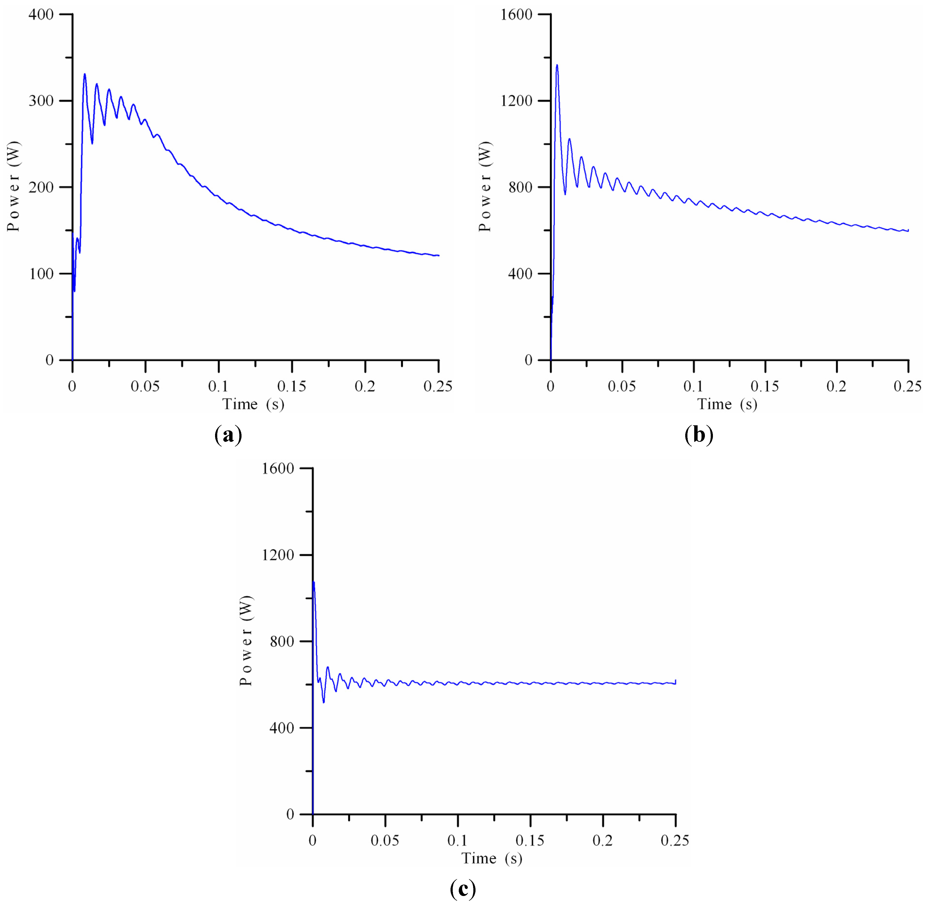
4.1. Case 1, EMTP Simulation

Case Study 1 of the NILM system identifies three loads with transient and steady-state signatures observed during the operation of a 480 V common bus. These loads include a 160 hp induction motor, a 123 hp induction motor driven by line frequency variable-voltage drives, and a hank of loads supplied by a six-pulse thyristor rectifier for AC power to simulate an exhaust fan, an air conditioning condenser, and DC lamps in commercial buildings, respectively.

Table 1 shows that training and test recognition accuracy values for load identification in multiple operations are 100% for real power and reactive power (PQ), P and Q and total harmonic distortion of voltage and current (PQV_THDI_THD), and transient response time and turn-on transient energy (t_TRU_T) as the power signatures. In the computation requirements of training time, the time of t_TRU_T is less than that of PQ or PQV_THDI_THD.

Table 1. The results of load identification in Case Study 1.

	Features	PQ		PQVTHDITHD		tTR UT (STFT)		tTR UT (DWT)
Items		Training	Test	Training	Test	Training	Test	Training	Test
Recognition Accuracy (%)		100	100	100	100	100	100	100	100
Time (s)		1.7845	0.00562	2.685	0.0058	1.0781	0.00566	1.0779	0.00565
Number of Iterations		123.1		224.3		80.1		79.7

Table 1. The results of load identification in Case Study 1.

	Features	PQ		PQVTHDITHD		tTR UT (STFT)		tTR UT (DWT)
Items		Training	Test	Training	Test	Training	Test	Training	Test
Recognition Accuracy (%)		100	100	100	100	100	100	100	100
Time (s)		1.7845	0.00562	2.685	0.0058	1.0781	0.00566	1.0779	0.00565
Number of Iterations		123.1		224.3		80.1		79.7

4.2. Case 2, EMTP Simulation for Different Loads with the Same Real Power and Reactive Power

The neural network in the NILM system of Case Study 2 identifies three loads with transient and steady-state signatures operating on a 220 V common bus. These loads include a 2.6 hp induction motor, a 4.7 hp induction motor, and an R-L linear load with P and Q equivalent to that of a 4.7 hp induction motor to simulate a fan, a washing machine, and a heater in a commercial building, respectively.

Figure 8 shows the turn-on instantaneous transient power waveforms of the three loads. Figure 8a,b clearly shows different turn-on transient waveforms for the small and medium-size induction motors. Although the cases in Figure 8b,c have the same powers for different loads; they show different turn-on instantaneous transient power waveforms.

Figure 8. Simulation of load turn-on instantaneous transient power for case 2. (a) a 2.6 hp induction motor; (b) a 4.7 hp induction motor; (c) an R-L linear load with P and Q equivalent to that of a 4.7 hp induction motor.

Figure 8. Simulation of load turn-on instantaneous transient power for case 2. (a) a 2.6 hp induction motor; (b) a 4.7 hp induction motor; (c) an R-L linear load with P and Q equivalent to that of a 4.7 hp induction motor.

Table 2 shows that the training and test recognition accuracy values for load identification in multiple operations are 100% and 92.1%, respectively, if the proposed t_TR and U_T are used for the DWT method. However, the training and test recognition accuracy of load identification in multiple operations are only 66.7% and 53.0%, respectively, if only P and Q are used. These loads do not have enough distinct characteristic harmonics, and the total harmonic distortion of voltage and current cannot improve the test recognition accuracy. The loads that cannot be identified by P and Q are the second and third loads, combinations of the first and second loads and combinations of the first and third loads. In other words, test recognition for those loads in multiple operations is quite low when using only P and Q as power signatures. The transient features t_TRU_T also require less training time than steady-state features.

Table 2. The results of load identification in Case Study 2.

	Features	PQ		PQVTHDITHD		tTR UT (STFT)		tTR UT (DWT)
Items		Training	Test	Training	Test	Training	Test	Training	Test
Recognition Accuracy (%)		66.667	53.030	85.56	60.683	96.970	83.333	100	92.121
Time (s)		14.2089	0.00567	19.56	0.0060	1.7895	0.00564	1.7888	0.00566
Number of Iterations		3000		3000		182.5		155.2

Table 2. The results of load identification in Case Study 2.

	Features	PQ		PQVTHDITHD		tTR UT (STFT)		tTR UT (DWT)
Items		Training	Test	Training	Test	Training	Test	Training	Test
Recognition Accuracy (%)		66.667	53.030	85.56	60.683	96.970	83.333	100	92.121
Time (s)		14.2089	0.00567	19.56	0.0060	1.7895	0.00564	1.7888	0.00566
Number of Iterations		3000		3000		182.5		155.2

4.3. Case 3, Experiment

The NILM system in Case Study 3 monitors the voltage and current waveforms of a three-phase electrical service entrance powering representative loads in a laboratory. The neural network algorithm in the NILM system identifies three actual loads with transient and steady-state signatures on a 220 V common bus. These loads include a three-phase R-L linear load, a one-phase 0.2 hp induction motor, and a three-phase 1 hp induction motor to simulate a heater, a fan, and an ice cube machine in a residential building, respectively.

The load in Figure 9a is a bank of three-phase R-L linear loads. The transient response time depends on the time constant of resistance and inductance. After three cycles, 0.05 s, the load current enters the steady state. The real power is approximately 5 kW.

Figure 9b,c shows a one-phase 0.2 hp induction motor and a three-phase 1 hp induction motor, respectively. These motors have different turn-on transient waveforms. The more horse power they have, the more current the induction motor requires to start.

Table 3 shows that the training recognition accuracy values of load identification in multiple operations can reach up to 100% when using PQ, PQV_THDI_THD, or t_TRU_T as the power signatures. In the test recognition accuracy of load identification, the values exceed 92% for PQ and other power signatures. The test recognition accuracy of the proposed DWT method for signature t_TRU_T is higher than that of other methods.

Table 3. The results of load identification in Case Study 3.

	Features	PQ		PQVTHDITHD		tTR UT (STFT)		tTR UT (DWT)
Items		Training	Test	Training	Test	Training	Test	Training	Test
Recognition Accuracy (%)		98.485	92.424	100	94.69	98.485	93.940	100	96.970
Time (s)		1.8502	0.00568	2.032	0.006	1.0782	0.00569	1.0783	0.00566
Number of Iterations		201.5		211.2		80.9		81.3

Table 3. The results of load identification in Case Study 3.

	Features	PQ		PQVTHDITHD		tTR UT (STFT)		tTR UT (DWT)
Items		Training	Test	Training	Test	Training	Test	Training	Test
Recognition Accuracy (%)		98.485	92.424	100	94.69	98.485	93.940	100	96.970
Time (s)		1.8502	0.00568	2.032	0.006	1.0782	0.00569	1.0783	0.00566
Number of Iterations		201.5		211.2		80.9		81.3

Figure 9. Experiment of load turn-on instantaneous transient power for case 3. (a) a three-phase R-L linear load; (b) a one-phase 0.2 hp induction motor; (c) a three-phase 1 hp induction motor.

Figure 9. Experiment of load turn-on instantaneous transient power for case 3. (a) a three-phase R-L linear load; (b) a one-phase 0.2 hp induction motor; (c) a three-phase 1 hp induction motor.

4.4. Case 4, Experiment for Different Loads with the Same Real Power and Reactive Power

The NILM system in Case Study 4 monitors the voltage and current waveforms of a one-phase electrical service entrance powering representative loads in a laboratory. The neural network algorithm in this NILM system identifies three actual loads with transient and steady-state signatures on a 110 V common bus. These loads include a 119 W dehumidifier, a 590 W vacuum cleaner, and an R-L linear load with P and Q equivalent to that of a 590 W vacuum cleaner.

Figure 10a,b clearly shows different turn-on transient waveforms for the different types of electrical equipment with induction motors. Figure 10b,c shows that the different loads have different instantaneous transient power waveforms even though they have identical P and Q.

Table 4 shows that the training and test recognition accuracy values for load identification in multiple operations exceed 98% and 83%, respectively, if the t_TR and the U_T are selected as the power signatures for the proposed DWT method. However, the training and test recognition accuracy of load identification in multiple operations are only 68.2% and 48.5%, respectively, when P and Q are selected. For the same reasons as those listed in Case Study 2, test recognition accuracy in multiple operations is quite low using only P and Q as power signatures. Because the loads in this case have sufficiently distinct harmonics, the total harmonic distortion of voltage and current can increase the test recognition accuracy when using PQV_THDI_THD as power signatures. In addition to recognition accuracy of load identification, the steady-state features require more computation time than transient features.

Figure 10. Experiment of load turn-on instantaneous transient power for case 4. (a) a 119 W dehumidifier; (b) a 590 W vacuum cleaner; (c) an R-L linear load with P and Q equivalent to that of a 590 W vacuum cleaner.

Figure 10. Experiment of load turn-on instantaneous transient power for case 4. (a) a 119 W dehumidifier; (b) a 590 W vacuum cleaner; (c) an R-L linear load with P and Q equivalent to that of a 590 W vacuum cleaner.

Table 4. The results of load identification in Case Study 4.

	Features	PQ		PQVTHDITHD		tTR UT (STFT)		tTR UT (DWT)
Items		Training	Test	Training	Test	Training	Test	Training	Test
Recognition Accuracy (%)		68.182	48.485	90.561	70.230	98.485	78.788	98.485	83.333
Time (s)		17.354	0.00567	20.542	0.0055	1.952	0.00561	1.885	0.00566
Number of Iterations		3000		3000		210.2		190.4

Table 4. The results of load identification in Case Study 4.

	Features	PQ		PQVTHDITHD		tTR UT (STFT)		tTR UT (DWT)
Items		Training	Test	Training	Test	Training	Test	Training	Test
Recognition Accuracy (%)		68.182	48.485	90.561	70.230	98.485	78.788	98.485	83.333
Time (s)		17.354	0.00567	20.542	0.0055	1.952	0.00561	1.885	0.00566
Number of Iterations		3000		3000		210.2		190.4

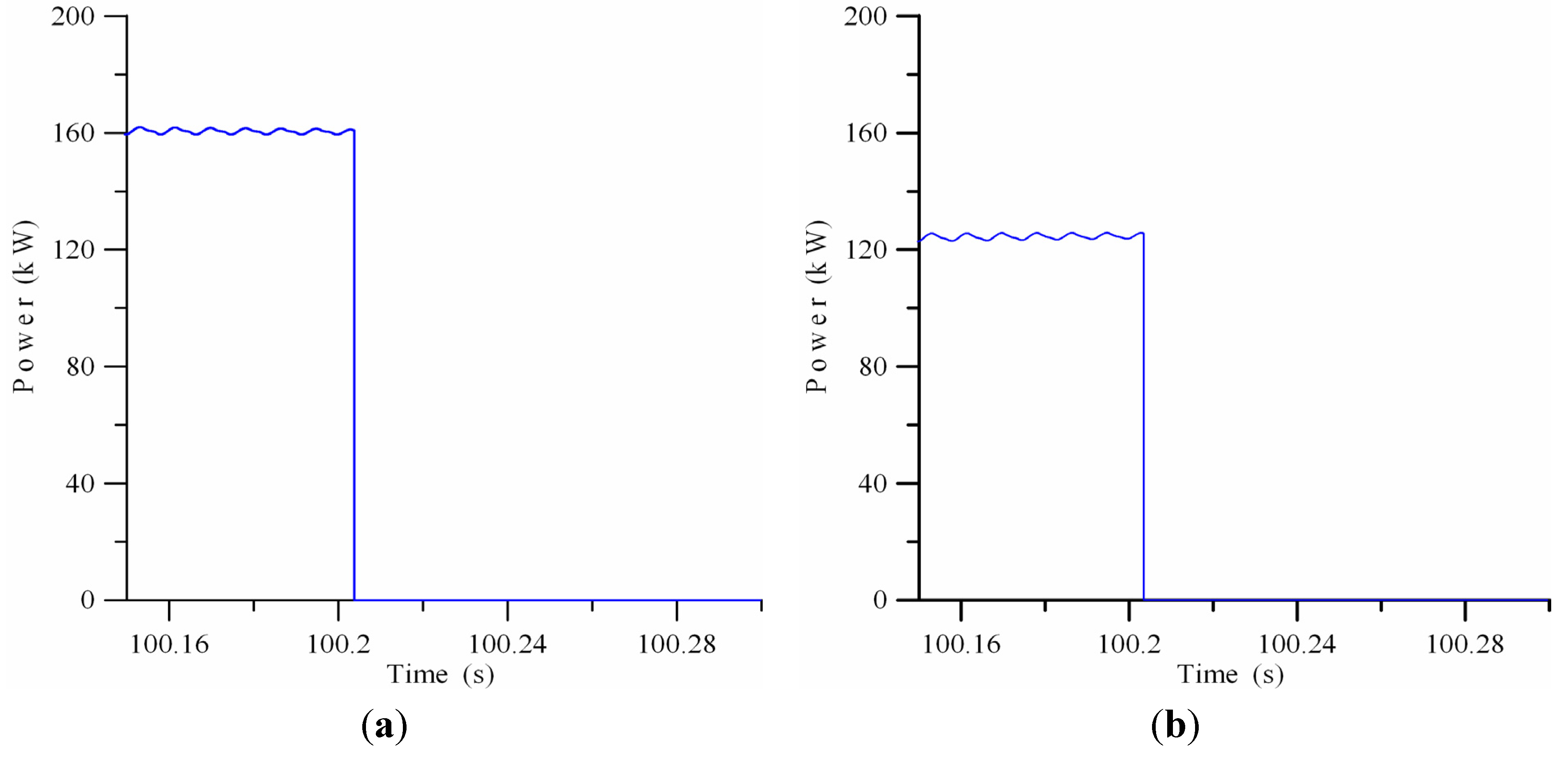
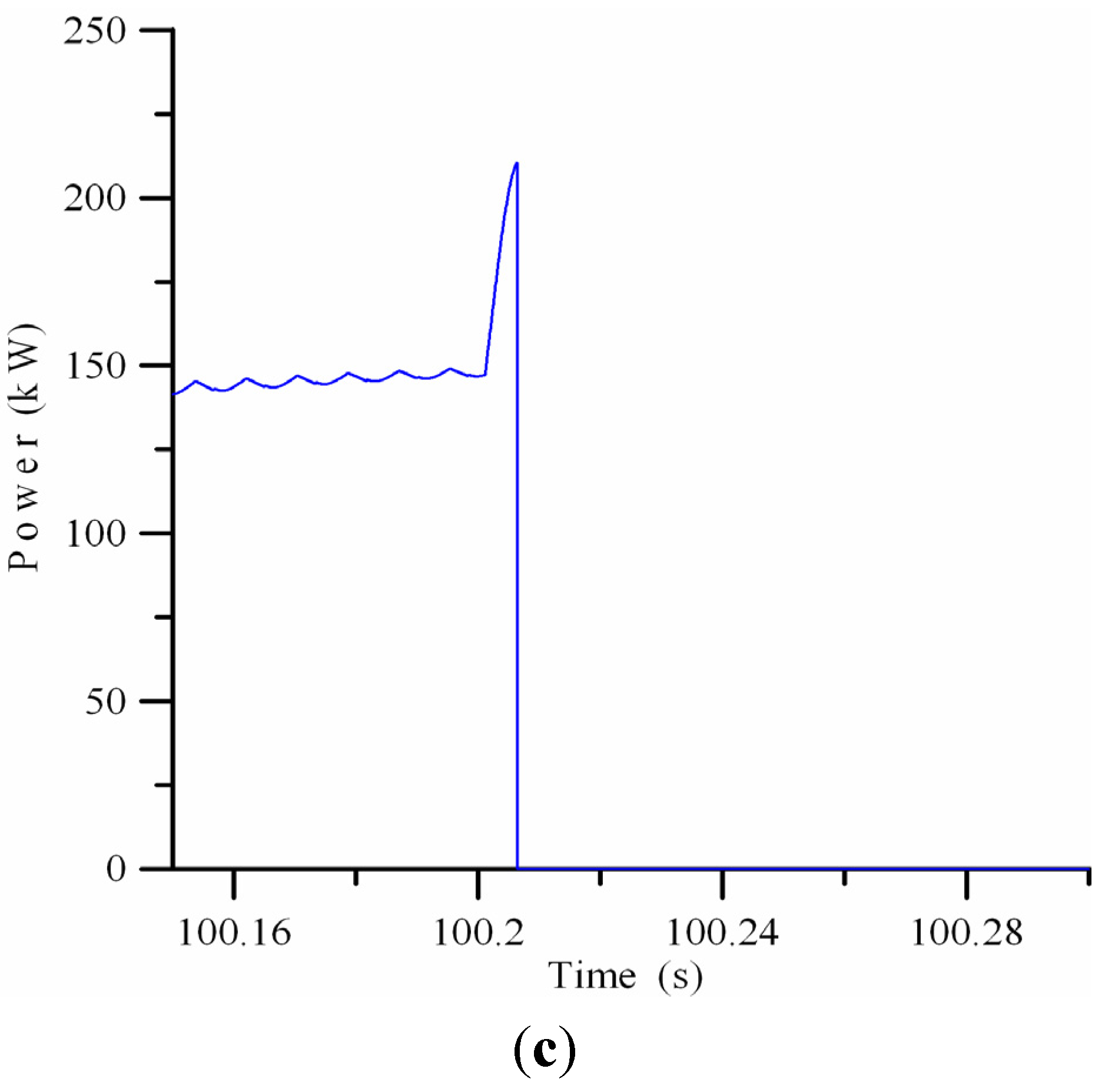
4.5. Case 5, Turn-off EMTP Simulation

A householder can know the power consumption of electrical load by observing the time of operation for each load monitored by an NILM system. When an undetermined electrical load is turned off, it is necessary to keep track of how often each electrical load is turned on and off. The neural network in the NILM system of Case Study 5 identifies three loads with transient and steady-state signatures observed during operation of a 480 V common bus. These loads are the same as those in Case Study 1. In this case study, the time of turning-off electrical loads is 100.2 s.

Figure 11 shows the turn-off instantaneous transient power waveforms of the three loads. The different turn-off instantaneous transient power waveforms in these figures clearly show different physical characteristics for these three loads. The loads in Figure 11a,b has different steady-state powers. The load in Figure 11c is combined with a bank of resistance and inductance driven by a six-pulse thyristor rectifier. The turn-off instantaneous transient power waveform of Figure 11c differs from that of Figure 11a,b because of the controller of the six-pulse thyristor rectifier.

Figure 11. The instantaneous power waveforms of turn-off transients. (a) a 160 hp induction motor; (b) a 123 hp induction motor driven by variable-voltage drives; (c) a bank of loads supplied by a six-pulse thyristor rectifier for AC power.

Figure 11. The instantaneous power waveforms of turn-off transients. (a) a 160 hp induction motor; (b) a 123 hp induction motor driven by variable-voltage drives; (c) a bank of loads supplied by a six-pulse thyristor rectifier for AC power.

Table 5 shows that the training and test recognition accuracy values of load identification in multiple operations are all 100% for the signatures of transient response time (t_TR) and turn-off transient energy (U_T-OFF). However, the analysis technique is the DWT or STFT.

Table 5. The Results of Load Identification in Case Study 5.

	Features	tTR UT-OFF (STFT)		tTR UT-OFF (DWT)
Items		Training	Test	Training	Test
Recognition Accuracy (%)		100	100	100	100
Time (s)		1.0578	0.0056	1.0385	0.00552
Number of Iterations		78.5		73.6

Table 5. The Results of Load Identification in Case Study 5.

	Features	tTR UT-OFF (STFT)		tTR UT-OFF (DWT)
Items		Training	Test	Training	Test
Recognition Accuracy (%)		100	100	100	100
Time (s)		1.0578	0.0056	1.0385	0.00552
Number of Iterations		78.5		73.6

5. Conclusions

The method proposed in this study allows a user to monitor the power consumption of electrical loads by observing the operation and time of use for loads monitored by the NILM. Furthermore, this allows users to improve their electricity consumption habits to save electricity energy and reduce carbon emissions from a viewpoint of power consumption in the future. In the analyses and comparisons of the transient analyses, this study compares and analyzes the results of the STFT and DWT of the turn-on transients of typical representative loads. Moreover, this study proposes transient features, including the transient response time and the transient energy, to be analyzed by the DWT for the power signatures. Experimental results show the transient features (t_TRU_T) are better than steady-state features for improving recognition accuracy and reducing the computation requirements of non-intrusive power demand morning and load identification.

References

1. Chang, H.H. Genetic algorithms and non-intrusive energy management system based economic dispatch for cogeneration units. Energy 2011, 36(1), 181–190. [Google Scholar] [CrossRef]
2. Hart, G.W. Nonintrusive appliance load monitoring. Proc. IEEE 1992, 80, 1870–1891. [Google Scholar] [CrossRef]
3. Langhman, C.; Lee, K.; Cox, R.; Show, S.; Leeb, S.B.; Norford, L.; Armstrong, P. Power signature analysis. IEEE Power & Energy Mag. 2003, 1(2), 56–63. [Google Scholar] [CrossRef]
4. Leeb, S.B. A Conjoint Pattern Recognition Approach to Nonintrusive Load Monitoring. Ph.D. Thesis, Massachusetts Institute of Technology, Cambridge, MA, USA, 1993. [Google Scholar]
5. Cole, A.I.; Albicki, A. Nonintrusive identification of electrical loads in a three-phase environment based on harmonic content. In Proceedings of 17th IEEE Instrumentation and Measurement Technology Conference, Baltimore, MD, USA, 1–4 May 2000; pp. 24–29.
6. Hong, Y.Y.; Chou, J.H. Nonintrusive energy monitoring for microgrids using hybrid self-organizing feature-mapping networks. Energies 2012, 5, 2578–2593. [Google Scholar] [CrossRef]
7. Cole, A.I.; Albicki, A. Data extraction for effective non-intrusive identification of residential power loads. In Proceedings of the IEEE Instrumentation and Measurement Technology Conference (IMTE/98), St. Paul, MN, USA, 18–21 May 1998; pp. 812–815.
8. Cole, A.I.; Albicki, A. Algorithm for non-intrusive identification of residential appliances. In Proceedings of the IEEE International Symposium on Circuits and Systems (ISCAS’98), Monterey Conference Center, Monterey, CA, USA, 31 May–3 June 1998; pp. 338–341.
9. Norford, L.K.; Leeb, S.B. Non-intrusive electrical load monitoring in commercial buildings based on steady-state and transient load-detection algorithm. Energy Build. 1996, 24, 51–64. [Google Scholar] [CrossRef]
10. Lee, K.D.; Leeb, S.B.; Norford, L.K.; Armstrong, P.R.; Holloway, J.; Shaw, S.R. Estimation of variable-speed-drive power consumption from harmonic content. IEEE Trans. Energy Convers. 2005, 20(3), 566–574. [Google Scholar] [CrossRef]
11. Shaw, S.R.; Leeb, S.B.; Norford, L.K.; Cox, R.W. Nonintrusive load monitoring and diagnostics in power systems. IEEE Trans. Instrum. Meas. 2008, 57(7), 1445–1454. [Google Scholar] [CrossRef]
12. Marceau, M.L.; Zmeureanu, R. Nonintrusive load disaggregation computer program to estimate the energy consumption of major end users in residential buildings. Energy Convers. Manag. 2000, 41, 1389–1403. [Google Scholar] [CrossRef]
13. Farinaccio, L.; Zmeureanu, R. Using a pattern recognition approach to disaggregate the total electricity consumption in a house into the major end-uses. Energy Build. 1999, 30, 245–259. [Google Scholar] [CrossRef]
14. Srinivasan, D.; Ng, W.S.; Liew, A.C. Neural-network-based signature recognition for harmonic source identification. IEEE Trans. Power Deliv. 2006, 21(1), 398–405. [Google Scholar] [CrossRef]
15. Roos, J.G.; Lane, I.E.; Lane, E.C.; Hanche, G.P. Using neural networks for non-intrusive monitoring of industrial electrical loads. In Proceedings of the IEEE Instrumentation and Measurement Technology Conference, Hamamatsu, Japan, 10–14 May 1994; pp. 1115–1118.
16. Chang, H.H.; Yang, H.T.; Lin, C.L. Load identification in neural networks for a non-intrusive monitoring of industrial electrical loads. Lect. Notes Comput. Sci. 2008, 5236, 664–674. [Google Scholar]
17. Zhao, C.; He, M.; Zhao, X. Analysis of transient waveform based on combined short time Fourier transform and wavelet transform. In Proceedings of the IEEE International Conference on Power System Technology, Singapore, 21–24 November 2004; pp. 1122–1126.
18. Robertson, D.C.; Camps, O.I.; Mayer, J.S.; Gish, W.B. Wavelets and electromagnetic power system transients. IEEE Trans. Power Deliv. 1996, 11(2), 1050–1056. [Google Scholar] [CrossRef]
19. Leeb, S.B.; Shaw, S.R.; Kirtly, J.L., Jr. Transient event detection in spectral envelop estimates for nonintrusive load monitoring. IEEE Trans. Power Deliv. 1995, 10(3), 1200–1210. [Google Scholar] [CrossRef]
20. Khan, U.A.; Leeb, S.B.; Lee, M.C. A multiprocessor for transient event detection. IEEE Trans. Power Deliv. 1997, 12(1), 51–60. [Google Scholar] [CrossRef]
21. Kosko, B. Neural Networks and Fuzzy Systems: A Dynamical Systems Approach to Machine Intelligence; Prentice-Hall: Englewood Cliff, NJ, USA, 1992. [Google Scholar]
22. Hong, Y.Y.; Chen, B.Y. Locating switched capacitor using wavelet transform and hybrid principal component analysis network. IEEE Trans. Power Deliv. 2007, 22(2), 1145–1152. [Google Scholar] [CrossRef]
23. Liao, C.C.; Yang, H.T.; Chang, H.H. Denoising techniques with a spatial noise-suppression method for wavelet-based power-quality monitoring. IEEE Trans. Instrum. Meas. 2011, 60(6), 1986–1996. [Google Scholar] [CrossRef]
24. Chang, H.H.; Chen, K.L.; Tsai, Y.P.; Lee, W.J. A new measurement method for power signatures of non-intrusive demand monitoring and load identification. IEEE Trans. Ind. Appl. 2012, 48(2), 764–771. [Google Scholar] [CrossRef]