Day-Ahead Electricity Price Forecasting Using a Hybrid Principal Component Analysis Network

Abstract

Bidding competition is one of the main transaction approaches in a deregulated electricity market. Locational marginal prices (LMPs) resulting from bidding competition and system operation conditions indicate electricity values at a node or in an area. The LMP reveals important information for market participants in developing their bidding strategies. Moreover, LMP is also a vital indicator for the Security Coordinator to perform market redispatch for congestion management. This paper presents a method using a principal component analysis (PCA) network cascaded with a multi-layer feedforward (MLF) network for forecasting LMPs in a day-ahead market. The PCA network extracts essential features from periodic information in the market. These features serve as inputs to the MLF network for forecasting LMPs. The historical LMPs in the PJM market are employed to test the proposed method. It is found that the proposed method is capable of forecasting day-ahead LMP values efficiently.

1. Introduction

There are two main transaction modes in a deregulated electric power industry, namely, competitive bidding and bilateral contract. Competitive biddings are used in the energy, spot, firm-transmission-right and ancillary service markets while bilateral contract is adopted outside the competitive market for any two individual entities, buyer and seller [1,2]. For either transaction mode, the electricity price information serves as an essential signal for all entities to adjust their offers/bids and/or contract prices. In particular, locational marginal pricing (LMP) is one of the most popular modes for pricing electricity in a deregulated electricity market. LMPs can reflect the electricity value at a node and may be discriminated at different nodes in a power network [3]. LMPs provide information that is helpful to market participants in developing their bidding strategies. It is also a vital indicator for the Security Coordinator to mitigate transmission congestion [4]. LMPs reveal important information for both the spot market and entities with bilateral contracts.

Past studies have investigated short-term System Marginal Price (SMP) forecasting [5,6]. Because the SMP is irrelevant to transmission constraints, forecasting LMPs subject to transmission constraints is more difficult than forecasting Market Clear Prices (MCPs). Current methods for short-term LMP forecasting can be classified at least into three groups: hour-ahead, day-ahead and week-ahead forecastings.

The recurrent neural network integrated with fuzzy-c-means was proposed for hour-ahead LMP forecasting in [7]. Linguistic descriptions in the PJM market were transformed into fuzzy membership functions associated with the recurrent neural network for forecasting volatile hour-ahead LMP variations when contingency occurs [8]. This paper investigates the more difficult problem related to the day-ahead price forecasting, which may be applied to the day-ahead market and will be discussed in the next paragraph.

In recent years, Contreras et al. [9] used the ARIMA model and Nogales et al. [10] used the dynamic regression approach and transfer function approach to predict the next-day (day-ahead) electricity prices. However, there is no discussion on extracting the market features for usage of these approaches in [9,10]. Li et al. [11] integrated the fuzzy inference system with least-squares estimation to conduct the day-ahead electricity price forecasting. The “week day”, “yesterday price” and “local demand” were considered in the 18 antecedent (premise or condition) parts of the fuzzy rules in [11]. Giving the membership functions of these three linguistic variables is quite heuristic. Moreover, the “local demand” for the fuzzy rules is not a forecasted but an actual value, which is generally not available in the day-ahead market. Amjady and Keynia [12] combined a mutual information technique (MIT) with the cascaded neuro-evolutionary algorithm (NEA) for the day-ahead electricity price forecasting. In [12], 14 features in the market were selected by MIT for 24 feedforward neural networks trained by the NEA. No reasonable explanation was found for these 14 features. Moreover, many (24) neural networks make the method impractical for industrial application. Garcia et al. [13] presented an approach to predicting next-day electricity prices using the Generalized Autoregressive Conditional Heteroskedastic (GARCH) methodology, which is an extended auto-regressive integrated moving average (ARIMA). Amjady [14] presented a fuzzy neural network with an inter-layer and feedforward architecture using a new hypercubic training mechanism. The proposed method predicted hourly market-clearing prices for the day-ahead electricity markets. Again, there is no discussion on extracting the market features for usage of the GARCH in [13,14]. Coelho and Santos [15] proposed a nonlinear forecasting model based on radial basis function neural networks (RBF-NNs) with Gaussian activation functions. Partial autocorrelation functions (PACF), which relies on the mutual linear dependency among studied parameters, was used to identify the market features. However, the relation among power market features is very nonlinear.

The problem of week-ahead price forecasting is generally easier than that of day-ahead price forecasting because the price pattern of a day is similar to that of its corresponding week-ahead day. Catalao et al. [16] proposed a wavelet-based Sugeno type fuzzy inference system to predict the electricity price in the electricity market of mainland Spain. However, the selection of numbers of membership functions in [16] is a trade-off between refining and sparseness. Che and Wang [17] presented a method based on support vector regression and ARIMA modeling; however, only the MCPs of California electricity market were used to examine the accuracy of the proposed method. The method has not been applied to forecasting LMPs, whose pattern is more nonlinear than MCPs’.

Because LMPs vary dramatically, it is difficult to analyze the related data with traditional techniques (e.g., regression analysis). Like other forecasting problems [18,19,20], the LMP forecasting needs feature extraction incorporating a powerful approach. As described above, the neural network is suitable for nonstationary time-series prediction, providing satisfactory results. In this paper, a principal component analysis (PCA) neural network cascaded with the multi-layer-feedforward (MLF) neural network is proposed for day-ahead LMP forecasting. The PCA neural network is used to extract essential features in the electricity market. It also helps reduce high-dimensional data into low-dimensional ones, which serve as inputs for the MLF neural network.

The rest of this paper is organized as follows: the PJM real-time market data will be described in Section 2. The proposed PCA neural network cascaded with the MLF neural network for forecasting day-ahead LMPs will be given in Section 3. Simulation results obtained using the PJM data are presented in Section 4. Concluding remarks are provided in Section 5.

2. Volatile LMPs in a Day-ahead Market

The PJM energy market comprises day-ahead and real-time markets. The day-ahead market is a forward market in which hourly LMPs are calculated for the next operating day using generation offers, demand bids and scheduled bilateral transactions. The real-time market is a spot market in which current LMPs are calculated at five-minute intervals according to actual grid operating conditions. PJM settles transactions hourly and issues invoices to market participants monthly. Figure 1 and Figure 2 illustrate the LMPs in Fisk (4 kV) and Byberry (13 kV), respectively, on 1–7 July 2008. As can be seen, LMPs vary dramatically over a wide range.

Figure 1. Daily LMPs in Fisk (4 kV) on 1–7 July 2008.

Figure 1. Daily LMPs in Fisk (4 kV) on 1–7 July 2008.

Figure 2. Daily LMPs in Byberry (13 kV) on 1–7 July 2008.

Figure 2. Daily LMPs in Byberry (13 kV) on 1–7 July 2008.

3. The Proposed Method

The hybrid PCA neural network is developed by combining the unsupervised PCA and supervised MLF neural networks to conduct day-ahead LMP forecasting. The PCA neural network is employed to extract essential features in the electricity market. The PCA neural network can also reduce high-dimensional data into low-dimensional ones, which serve as inputs of the MLF neural network to reduce the training CPU time.

3.1. Principal Component Analysis Neural Network

The purpose of the PCA neural network is to find a set of P orthonormal vectors (OVs) in a Q-dimensional space (Q ≥ P), such that these OVs will account for as much variance of the input data as possible. OVs are actually P eigenvectors associated with the P largest eigenvalues of the E($x{x}^t$), where x denotes the Q-dimensional input column vector, i.e., x = (x₁ x₂ … x_Q)^t. The direction of the q-th principal component will be along the q-th eigenvector, q = 1, 2, .., Q.

Let symbol t be the training index. This paper used Sanger’s method [21] to update the weightings between the neurons of the PCA network as follows:

$$\Delta w_p(t)=\eta (t)v_p(t)\left(x(t)-{\displaystyle \sum _{pj=1}^p{v}_{pj}(t)w_{pj}(t)}\right),p=1, 2, \dots , \text{P}$$

(1)

where $\eta (t)$ is a parameter of learning rate and $v_{pj}(t)=w_{pj}^t(t)x(t)$ is the output. Equation (1) is employed to train a neural network consisting of P linear neurons so as to find the first P principal components. More specifically, Generalized Hebbian Algorithm was able to make $w_p(t),$ p = 1, 2, …, P, converge to the first P principal component directions, in sequential order: $w_p(t)\to \pm v_i,$ where v_i is a normalized eigenvector associated with the i-th largest eigenvalue of the correlation matrix. It was shown that if $w_{pj}(t),$ pj = 1, 2, …, p − 1 have converged to $v_{pj}(t),$ pj = 1, 2, …, p − 1, respectively, then the maximal eigenvalue ${\lambda }_p$ and the corresponding normalized eigenvector $v_p$ of the correlation matrix of x_p, i.e., C_p ≡ E($x_p{x}_p^t$), are exactly the p-th eigenvalue and the p-th normalized eigenvector $v_p$ of the correlation matrix of x, i.e., C ≡ E($x{x}^t$), respectively. Consequently, neuron p can find the p-th normalized eigenvector of C. Detailed explanations can be found in [21].

It was shown that $\eta (t)$ should be smaller than the reciprocal largest eigenvalue of E(xx^t) to ensure the convergence of training a PCA neural network. When the training process is convergent, $w_p$, p = 1, 2, …, P, converges to the p-th eigenvector of E(xx^t).

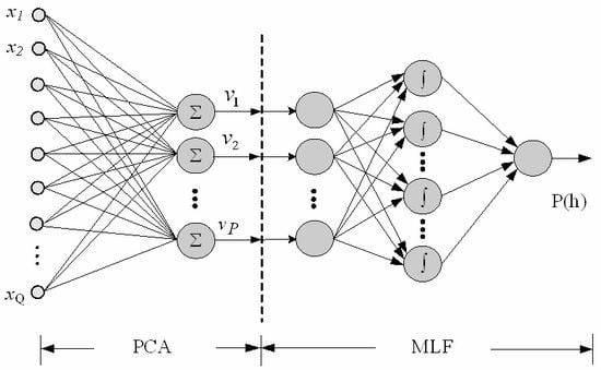
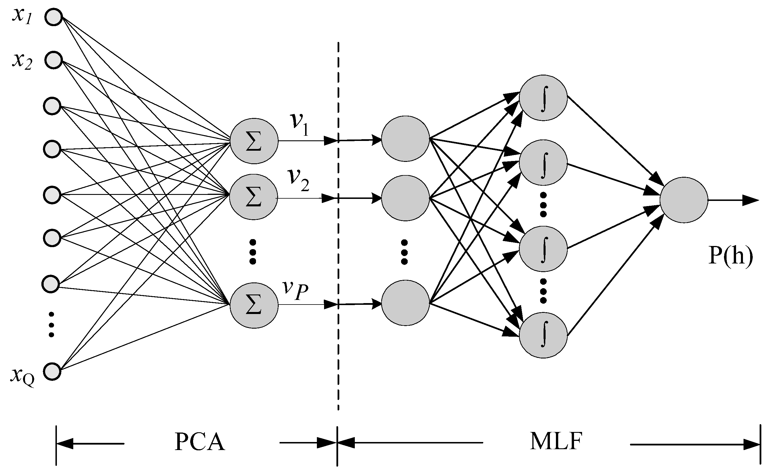
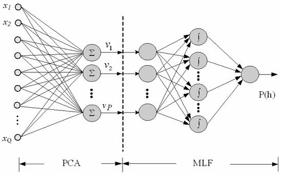
Figure 3 shows the configuration of the hybrid PCA neural network: The left part of Figure 3 is the unsupervised PCA neural network while the right part is the supervised MLF neural network. Because the training time of unsupervised PCA neural network is trivial while that of supervised MLF is considerable, PCA neural network is adopted to reduce both the dimension of training data and the training time for the cascaded MLF network trained by the back-propagation algorithm, which is well known and ignored here.

In the proposed hybrid PCA, the new hidden layer consists of 20 neurons. The number (p) of orthonormal vectors is 24 or 48, depending on the numbers of inputs. After training the unsupervised PCA, the supervised MLF is trained, using the frozen weights of the unsupervised PCA. The training sets are identical for both unsupervised and supervised NNs.

Figure 3. The proposed hybrid PCA neural network.

Figure 3. The proposed hybrid PCA neural network.

3.2. Features for Inputs of PCA Neural Network

The performance of a neural network depends strongly on the adopted features at the input layers. As shown in Figure 1 and Figure 2, variations of system load affect LMPs. Assume that the h-th LMP is to be forecasted. Let P(h) and L(h) be the LMP and MW demand at hour h, respectively.

Below are 4 alternatives for considering input features x₁, x₂, …, x_Q:

(1)

The features of the past 2 days: F1(h) ≡ (P(h − 47), P(h − 46), …, P(h − 25), P(h − 24) and L(h − 47), L(h − 46), …, L(h − 25), L(h − 24)). That is, Q = 48.

(2)

The features of the same day of the last week and those of the past 2 days: F2(h) ≡ (P(h − 168), P(h − 167), …, P(h − 146), P(h − 145), P(h − 47), P(h − 46), …, P(h − 25), P(h − 24) and L(h − 168), L(h − 167), …, L(h − 146), L(h − 145), L(h − 47), L(h − 46), …, L(h − 25), L(h − 24)). That is, Q = 96.

(3)

The features of the past 2 days and the designated day: F3(h) = F1(h) ∪ (D|D is one of the seven days in a week). This implies Q = 49.

(4)

The features of the same day of the last week, those of the past 2 days and the designated day: F4(h) = F2(h) ∪ (D|D is one of the seven days in a week). This means Q = 97.

The symbol D for the designated day here means Monday, …, Saturday or Sunday. Because the neural network cannot deal with symbols, 30, 50, …, 150 stand for Monday, …, Saturday and Sunday, respectively, in this paper.

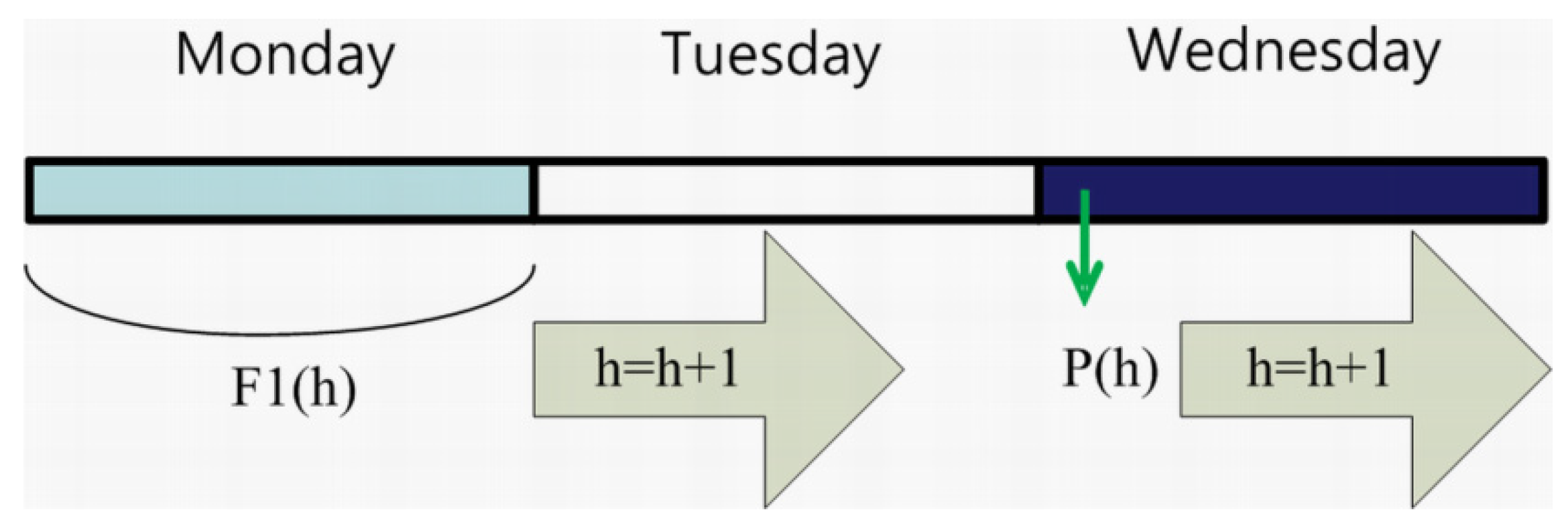
3.3. Moving Data Windows for Forecasting

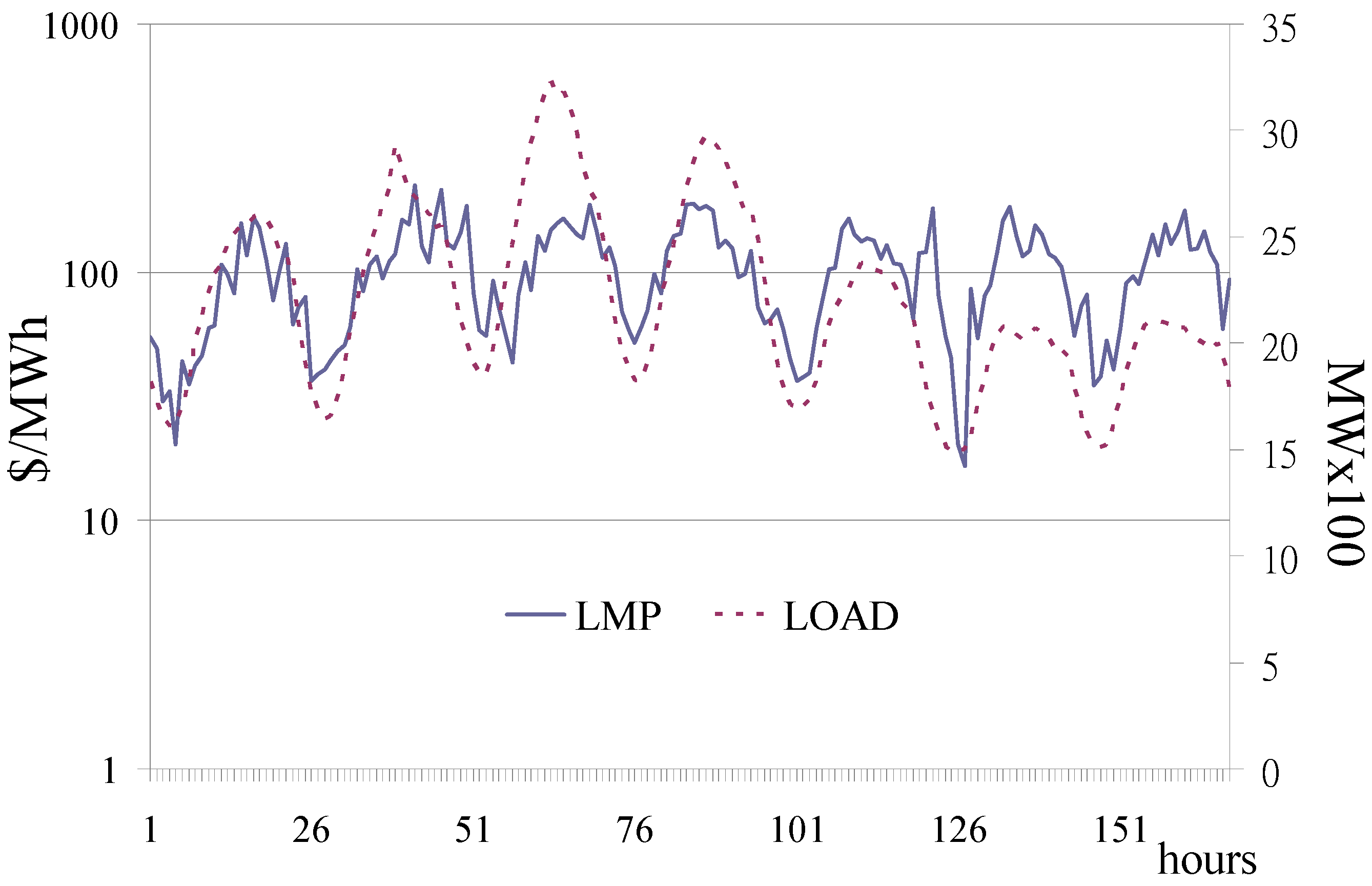
P(h) at the output layer is paired with F1(h), F2(h), F3(h) or F4(h). More specifically, assume that F1(h) is considered and the 24 LMPs on Wednesday (next day) are forecasted. Figure 4 illustrates the moving data window corresponding to the forecasted LMP. Hence, the paired training data are as follows: (F1(h), P(h)), (F1(h + 1), P(h + 1)), …, (F1(h + 23), P(h + 23)). In Figure 4, the first data set involves only Monday and Wednesday. The last 23 data on Monday and the first data on Tuesday will be paired with P(h + 1) for the second data set. Restated, forecasting 24 LMPs on Wednesday will be completed at 23:00 p.m. on Tuesday.

When the proposed hybrid PCA neural network is used in the day-ahead market or in the testing stage, the input data for the past day (e.g., Monday in Figure 4) and this day (e.g., Tuesday in Figure 4) are known and output (forecasted) data for the next day (e.g., Wednesday in Figure 4) is unknown.

Figure 4. Moving data window (F1(h)) corresponding to forecasted P(h).

Figure 4. Moving data window (F1(h)) corresponding to forecasted P(h).

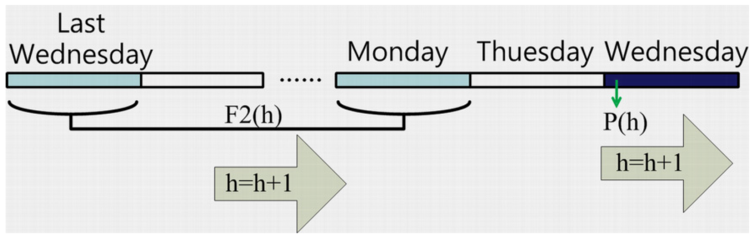
Assume that this day is Tuesday and LMPs on Wednesday are to be forecasted. Figure 5 shows the moving data window for F2(h) paired with P(h). The paired training data are as follows: (F2(h), P(h)), (F2(h + 1), P(h + 1)), …, (F2(h + 23), P(h + 23)). As shown in Figure 5, the first data set involves only the last Wednesday, Monday and Wednesday. The time index h will be increased by one at a time until h + 23. Restated, forecasting 24 LMPs on Wednesday will be completed at 23:00 p.m. on Tuesday.

Figure 5. Moving data window (F2(h)) corresponding to forecasted P(h).

Figure 5. Moving data window (F2(h)) corresponding to forecasted P(h).

3.4. Numbers of Neurons in Different Layers

The numbers of input, output, second, and fourth layers are discussed as follows:

(1)

The numbers of input neurons for the hybrid PCA neural networks are 48, 96, 49 and 97 for F1(h), F2(h), F3(h) and F4(h), respectively. That is, subscript Q in Figure 3 can be 48, 96, 49 or 97.

(2)

The number of neurons in the MLF output layer is one (i.e., P(h)), regardless of F1(h), F2(h), F3(h) and F4(h) being considered.

(3)

Because the purpose of the PCA neural network is to find a set of P orthonormal vectors (OVs) in a Q-dimensional space, P is expected to be smaller than the corresponding number of inputs. It is intuitive to consider P in Figure 3 to be 24 for the studied problem with Q = 48 or 49 because there are 24 hours in a day. Similarly, P = 48 while Q = 96 or 97.

(4)

The common number of neurons for the fourth (hidden) layer is (P + number of output neurons)/2 or (P × number of output neurons)^0.5. The simulation results show no significant difference between these two alternatives.

4. Simulation Results

In order to demonstrate the applicability of the proposed hybrid PCA neural network, the LMPs for the Fisk (4 kV) and Byberry (13 kV) areas in the PJM system were studied. Two sets of 366 × 24 data (1 January–31 December 2008) for Fisk and Byberry from the PJM web site were employed to train/validate and test the proposed hybrid PCA neural network. The entire data set includes four seasons. The data of each season are further divided into three groups: training data, validation data (in total 2/3), and test data (1/3). The training data were used for training the neural network and updating the biases and weights. The validation data were utilized to monitor the training process. The remaining data were employed to test the proposed hybrid PCA neural network after they were well trained. A C++ code was developed using a PC equipped with a Pentium(R) Dual-Core E5200 2.5 GHz CPU and 4-GB RAM for showing the applicability of the proposed method.

4.1. Comparison between Hybrid PCA and Back Propagation-Based Neural Networks

In this subsection, the performance of the proposed hybrid PCA neural network is compared with that of traditional back propagation-based (BP-based) neural network for the Fisk area. The traditional BP-based neural network can be taken as a neural network in which there are no second and third layers as seen in Figure 3. Table 1, Table 2, Table 3 and Table 4 display the CPU time (minute: second), correlation coefficient (R2) and mean absolute error (MAE, $/MWh) obtained by these two methods for Fisk. The correlation coefficient represents the resemblance between the actual and the forecasted values. The value of one for the correlation coefficient indicates that the actual values are identical to the forecasted ones. The average value and corresponding standard deviation (sd, $/MWh) of actual LMPs in each season are also shown in the second and third columns of Table 1, Table 2, Table 3 and Table 4 . Figure 6 shows the comparisons among actual, BP-based and hybrid PCA-based LMPs for Fisk (1–7 July 2008).

Table 1. Performance comparison between the proposed hybrid PCA and BP-based neural network (Fisk, spring).

Dimension of input vector	LMP ($/MWh)		Hybrid PCA Network			BP-based Network
Q	average	sd	time	R2	MAE	time	R2	MAE
48	52.89	25.17	03:50	0.749	14.96	04:21	0.707	15.85
49			03:36	0.814	13.11	04:28	0.777	14.72
96			06:20	0.838	14.19	07:05	0.767	15.19
97			06:34	0.838	13.78	08:19	0.769	15.10

Table 1. Performance comparison between the proposed hybrid PCA and BP-based neural network (Fisk, spring).

Dimension of input vector	LMP ($/MWh)		Hybrid PCA Network			BP-based Network
Q	average	sd	time	R2	MAE	time	R2	MAE
48	52.89	25.17	03:50	0.749	14.96	04:21	0.707	15.85
49			03:36	0.814	13.11	04:28	0.777	14.72
96			06:20	0.838	14.19	07:05	0.767	15.19
97			06:34	0.838	13.78	08:19	0.769	15.10

Table 2. Performance comparison between the proposed hybrid PCA and BP-based neural network (Fisk, summer).

Dimension of input vector	LMP ($/MWh)		Hybrid PCA Network			BP-based Network
Q	average	sd	time	R2	MAE	time	R2	MAE
48	55.61	40.52	04:06	0.793	21.35	04:35	0.759	21.36
49			04:39	0.823	20.68	04:50	0.800	21.42
96			08:48	0.826	21.15	12:00	0.824	21.16
97			08:53	0.843	20.51	12:59	0.829	20.74

Table 2. Performance comparison between the proposed hybrid PCA and BP-based neural network (Fisk, summer).

Dimension of input vector	LMP ($/MWh)		Hybrid PCA Network			BP-based Network
Q	average	sd	time	R2	MAE	time	R2	MAE
48	55.61	40.52	04:06	0.793	21.35	04:35	0.759	21.36
49			04:39	0.823	20.68	04:50	0.800	21.42
96			08:48	0.826	21.15	12:00	0.824	21.16
97			08:53	0.843	20.51	12:59	0.829	20.74

Table 3. Performance comparison between the proposed hybrid PCA and BP-based neural network (Fisk, fall).

Dimension of input vector	LMP ($/MWh)		Hybrid PCA Network			BP-based Network
Q	average	sd	time	R2	MAE	time	R2	MAE
48	53.23	32.43	03:45	0.840	15.57	04:50	0.840	16.42
49			03:55	0.858	15.34	04:55	0.847	15.81
96			13:41	0.901	13.06	14:34	0.875	16.22
97			13:55	0.904	13.66	14:44	0.876	15.42

Table 3. Performance comparison between the proposed hybrid PCA and BP-based neural network (Fisk, fall).

Dimension of input vector	LMP ($/MWh)		Hybrid PCA Network			BP-based Network
Q	average	sd	time	R2	MAE	time	R2	MAE
48	53.23	32.43	03:45	0.840	15.57	04:50	0.840	16.42
49			03:55	0.858	15.34	04:55	0.847	15.81
96			13:41	0.901	13.06	14:34	0.875	16.22
97			13:55	0.904	13.66	14:44	0.876	15.42

Table 4. Performance comparison between the proposed hybrid PCA and BP-based neural network (Fisk, winter).

Dimension of input vector	LMP ($/MWh)		Hybrid PCA Network			BP-based Network
Q	average	sd	time	R2	MAE	time	R2	MAE
48	42.36	19.15	03:53	0.706	11.02	04:16	0.683	12.19
49			03:57	0.765	10.69	04:24	0.725	12.58
96			08:03	0.818	10.13	12:26	0.786	10.71
97			08:21	0.822	10.03	12:40	0.780	11.28

Table 4. Performance comparison between the proposed hybrid PCA and BP-based neural network (Fisk, winter).

Dimension of input vector	LMP ($/MWh)		Hybrid PCA Network			BP-based Network
Q	average	sd	time	R2	MAE	time	R2	MAE
48	42.36	19.15	03:53	0.706	11.02	04:16	0.683	12.19
49			03:57	0.765	10.69	04:24	0.725	12.58
96			08:03	0.818	10.13	12:26	0.786	10.71
97			08:21	0.822	10.03	12:40	0.780	11.28

Figure 6. Comparisons among actual, BP-based and hybrid PCA-based LMPs for Fisk.

Figure 6. Comparisons among actual, BP-based and hybrid PCA-based LMPs for Fisk.

According to Table 1, Table 2, Table 3 and Table 4 , the following comments can be made:

(1)

The most volatile LMPs with an average of 55.61 $/MWh and a standard deviation of 40.52 $/MWh occurred in summer. The most steady LMPs with an average of 42.36 $/MWh and a standard deviation of 19.15 $/MWh occurred in winter.

(2)

For the same neural network, the R2 obtained by 49 inputs is better (larger) than that by 48 inputs; for the same reason, the neural network with 97 inputs has better performance than that with 96 inputs in terms of R2.

(3)

For the same neural network, the R2 obtained by 96 (97) inputs is much better (larger) than that by 48 (49) inputs; however, the CPU times required by 96 (97) inputs are longer.

(3)

For the same number of inputs, the R2 and MAE $/MWh obtained by the hybrid PCA neural network are better than those obtained by the BP-based neural network.

(4)

For the same number of inputs, the CPU time required by the hybrid PCA neural is shorter than that required by the BP-based neural network.

Table 5, Table 6, Table 7 and Table 8 show the comparison of performance between the proposed hybrid PCA neural network and the traditional BP-based neural network for the Byberry area. The same conclusions can be made for both Byberry and Fisk areas. Figure 7 shows the comparisons among actual, BP-based and hybrid PCA-based LMPs for Byberry (1–7 July 2008).

Table 5. Performance comparison between the proposed hybrid PCA and BP-based neural network (Byberry, spring).

Dimension of input vector	LMP ($/MWh)		Hybrid PCA Network			BP-based Network
Q	average	sd	time	R2	MAE	time	R2	MAE
48	73.95	42.05	03:28	0.681	25.89	04:01	0.634	28.15
49			03:39	0.734	25.41	04:05	0.669	28.56
96			06:00	0.784	24.60	07:05	0.673	28.40
97			06:07	0.793	24.22	07:35	0.681	29.22

Table 5. Performance comparison between the proposed hybrid PCA and BP-based neural network (Byberry, spring).

Dimension of input vector	LMP ($/MWh)		Hybrid PCA Network			BP-based Network
Q	average	sd	time	R2	MAE	time	R2	MAE
48	73.95	42.05	03:28	0.681	25.89	04:01	0.634	28.15
49			03:39	0.734	25.41	04:05	0.669	28.56
96			06:00	0.784	24.60	07:05	0.673	28.40
97			06:07	0.793	24.22	07:35	0.681	29.22

Table 6. Performance comparison between the proposed hybrid PCA and BP-based neural network (Byberry, summer).

Dimension of input vector	LMP ($/MWh)		Hybrid PCA Network			BP-based Network
Q	average	sd	time	R2	MAE	time	R2	MAE
48	87.22	52.73	03:41	0.797	28.06	04:32	0.789	28.15
49			03:52	0.842	26.36	04:58	0.827	26.96
96			08:25	0.859	25.10	14:47	0.852	25.73
97			08:30	0.868	24.37	14:51	0.848	26.50

Table 6. Performance comparison between the proposed hybrid PCA and BP-based neural network (Byberry, summer).

Dimension of input vector	LMP ($/MWh)		Hybrid PCA Network			BP-based Network
Q	average	sd	time	R2	MAE	time	R2	MAE
48	87.22	52.73	03:41	0.797	28.06	04:32	0.789	28.15
49			03:52	0.842	26.36	04:58	0.827	26.96
96			08:25	0.859	25.10	14:47	0.852	25.73
97			08:30	0.868	24.37	14:51	0.848	26.50

Table 7. Performance comparison between the proposed hybrid PCA and BP-based neural network (Byberry, fall).

Dimension of input vector	LMP ($/MWh)		Hybrid PCA Network			BP-based Network
Q	average	sd	time	R2	MAE	time	R2	MAE
48	88.41	50.30	03:08	0.765	25.01	04:15	0.725	25.66
49			03:15	0.769	24.73	04:36	0.761	25.24
96			08:06	0.848	23.48	11:41	0.823	23.59
97			08:11	0.874	23.17	11:54	0.864	23.62

Table 7. Performance comparison between the proposed hybrid PCA and BP-based neural network (Byberry, fall).

Dimension of input vector	LMP ($/MWh)		Hybrid PCA Network			BP-based Network
Q	average	sd	time	R2	MAE	time	R2	MAE
48	88.41	50.30	03:08	0.765	25.01	04:15	0.725	25.66
49			03:15	0.769	24.73	04:36	0.761	25.24
96			08:06	0.848	23.48	11:41	0.823	23.59
97			08:11	0.874	23.17	11:54	0.864	23.62

Table 8. Performance comparison between the proposed hybrid PCA and BP-based neural network (Byberry, winter).

Dimension of input vector	LMP ($/MWh)		Hybrid PCA Network			BP-based Network
Q	average	sd	time	R2	MAE	time	R2	MAE
48	56.73	25.26	03:28	0.725	14.72	04:29	0.688	14.98
49			03:58	0.779	13.94	04:53	0.709	15.24
96			09:53	0.830	12.96	11:22	0.754	13.62
97			09:58	0.837	12.99	11:54	0.757	16.03

Table 8. Performance comparison between the proposed hybrid PCA and BP-based neural network (Byberry, winter).

Dimension of input vector	LMP ($/MWh)		Hybrid PCA Network			BP-based Network
Q	average	sd	time	R2	MAE	time	R2	MAE
48	56.73	25.26	03:28	0.725	14.72	04:29	0.688	14.98
49			03:58	0.779	13.94	04:53	0.709	15.24
96			09:53	0.830	12.96	11:22	0.754	13.62
97			09:58	0.837	12.99	11:54	0.757	16.03

Figure 7. Comparisons among actual, BP-based and hybrid PCA-based LMPs for Byberry.

Figure 7. Comparisons among actual, BP-based and hybrid PCA-based LMPs for Byberry.

4.2. Investigation of Number of Output Neurons for PCA Network

The second layer of the proposed hybrid PCA neural network shown in Figure 3 denotes the features of the electricity market. The number (i.e., P) of neurons at this layer hence plays a crucial role in developing the proposed method. Table 9 and Table 10 show the impact of different P’s at the second layer on R2 and MAE for Fisk and Byberry areas, respectively, in fall. In order to show the effectiveness of the proposed method, only 97 inputs (i.e., Q) in Figure 3 were studied. The following remarks can be made according to Table 9 and Table 10:

(1)

The larger the P, the longer the CPU time is required due to the supervised MLF neural network at the third, fourth and fifth layers in Figure 3.

(2)

A larger P will result in a better performance in terms of R2 and MAE obtained. Hence, there is a trade-off between performance and CPU time. In general, performance is more important.

Table 9. Comparison between different P’s when Q = 97 (Fisk, fall).

P	CPU	R2	MAE
48	13:55	0.904	13.66
36	04:28	0.896	13.86
24	03:37	0.890	13.91
12	02:48	0.863	15.01

Table 9. Comparison between different P’s when Q = 97 (Fisk, fall).

P	CPU	R2	MAE
48	13:55	0.904	13.66
36	04:28	0.896	13.86
24	03:37	0.890	13.91
12	02:48	0.863	15.01

Table 10. Comparison between different P’s when Q = 97 (Byberry, fall).

P	CPU	R2	MAE
48	08:11	0.874	23.17
36	07:47	0.840	23.94
24	06:25	0.826	23.95
12	05:52	0.811	23.99

Table 10. Comparison between different P’s when Q = 97 (Byberry, fall).

P	CPU	R2	MAE
48	08:11	0.874	23.17
36	07:47	0.840	23.94
24	06:25	0.826	23.95
12	05:52	0.811	23.99

4.3. Comparison between Hybrid PCA Network and ARIMA

Traditional nonstationary time-series prediction method using ARIMA [9] is employed to study the same PJM day-ahead market. Because the hybrid PCA neural network with 97 inputs gained the best performance as described in Section 4.1, it was compared with the ARIMA. The general ARIMA formulation was given as follows [9]: φ(B)P(h) = θ(B)ε(h) where P(h) is the LMP at time h, φ(B) and $\theta (B)$ are functions of the backshift operator B: B_kP(h) ≡ P(h − k), and ε(h) () is the error term. This paper adopted the functions φ(B) and θ(B) given in [9] for comparisons. In [9], the load factor was not considered as a regressor in the ARIMA. Twenty four LMPs were used as lagged regressors in the ARIMA. Table 11 and Table 12 show the correlation coefficient (R2) and mean absolute error (MAE, $/MWh) obtained for all four seasons by the two methods.

The following comments could be made according to the results shown in Table 11 and Table 12:

(1)

For either Fisk or Byberry, the performances of the proposed hybrid PCA neural network are always better than those of the ARIMA in terms of both R2 and MAE obtained.

(2)

The R2’s obtained by the ARIMA for both Fisk and Byberry in winter are very low (0.488 and 0.419) while those obtained by the proposed method are much higher (0.822 and 0.837).

(3)

The LMPs in the Byberry area are more volatile than those in the Fisk area in terms of average R2 (0.566 with respect to 0.725). However, the proposed method is more reliable regardless of the studied areas; that is, 0.843 for Byberry is close to 0.852 for Fisk.

Table 11. Comparison between the proposed hybrid PCA and ARIMA [9] (Fisk).

Seasons	Hybrid PCA Network		ARIMA [9]
	R2	MAE	R2	MAE
Spring	0.838	13.78	0.808	15.89
Summer	0.843	20.51	0.757	21.33
Autumn	0.904	13.66	0.846	16.31
Winter	0.822	10.03	0.488	11.68
Average	0.852	14.50	0.725	16.30

Table 11. Comparison between the proposed hybrid PCA and ARIMA [9] (Fisk).

Seasons	Hybrid PCA Network		ARIMA [9]
	R2	MAE	R2	MAE
Spring	0.838	13.78	0.808	15.89
Summer	0.843	20.51	0.757	21.33
Autumn	0.904	13.66	0.846	16.31
Winter	0.822	10.03	0.488	11.68
Average	0.852	14.50	0.725	16.30

Table 12. Comparison between the proposed hybrid PCA and ARIMA [9] (Byberry).

Seasons	Hybrid PCA Network		ARIMA [9]
	R2	MAE	R2	MAE
Spring	0.793	24.22	0.578	28.10
Summer	0.868	24.37	0.743	27.81
Autumn	0.874	23.17	0.522	26.86
Winter	0.837	12.99	0.419	15.04
Average	0.843	21.19	0.566	24.45

Table 12. Comparison between the proposed hybrid PCA and ARIMA [9] (Byberry).

Seasons	Hybrid PCA Network		ARIMA [9]
	R2	MAE	R2	MAE
Spring	0.793	24.22	0.578	28.10
Summer	0.868	24.37	0.743	27.81
Autumn	0.874	23.17	0.522	26.86
Winter	0.837	12.99	0.419	15.04
Average	0.843	21.19	0.566	24.45

4.4. Diebold and Mariano Test

Diebold and Mariano proposed and evaluated explicit tests of the null hypothesis of no difference in the accuracy of two competing forecasts [22]. The loss function does not need to be quadratic, and even to be symmetric, and forecast errors can be non-Gaussian, nonzero mean, serially correlated, and contemporaneously correlated in this method. This subsection utilizes Diebold and Mariano test to evaluate the performance of the proposed hybrid PCA network, the BP-based network, and ARIMA. The loss function used in this paper is based on “mean squared error” (MSR) [23].

Let H₀ be the null hypothesis of no difference in the accuracy of the proposed hybrid PCA network and the BP-based network. The alternative hypothesis is the union of H₁ and H₂, which mean that the proposed hybrid PCA network is significantly better than the BP-based network and that the BP-based network is significantly better than the proposed hybrid PCA network, respectively. Under the null hypothesis, the test statistic S₁ defined in [22] and used to test H₀, H₁ and H₂ has an asymptotic standard normal distribution. Let the confidence level be 95%. If S₁ is greater than 1.96, than H₁ is accepted and H₀ is declined. If S₁ is smaller than −1.96, than H₂ is accepted and H₀ is declined. When S₁ is within [−1.96, 1.96], H₀ is accepted and there is no significant difference in forecasting accuracy between the two models. According to Table 13 and Table 14, the proposed hybrid PCA network has better performance in 9 out of 16 tests while 7 tests accept H₀. H₂ has never been accepted.

Similarly, Diebold and Mariano test is conducted to compare the performance between the proposed hybrid PCA network and ARIMA. Based on the same comparisons given in Table 11 and Table 12, Table 15 shows that the proposed hybrid PCA network is significantly better than ARIMA.

Table 13. Diebold and Mariano test between the proposed hybrid PCA and BP-based neural network (Fisk).

Seasons	Number of Input Q	S1	Results
spring	48	2.8701	accept H1, decline H0
	96	3.2559	accept H1, decline H0
summer	48	1.5524	accept H0
	96	0.2173	accept H0
fall	48	0.7640	accept H0
	96	3.4976	accept H1, decline H0
winter	48	3.1032	accept H1, decline H0
	96	3.1033	accept H1, decline H0

Table 13. Diebold and Mariano test between the proposed hybrid PCA and BP-based neural network (Fisk).

Seasons	Number of Input Q	S1	Results
spring	48	2.8701	accept H1, decline H0
	96	3.2559	accept H1, decline H0
summer	48	1.5524	accept H0
	96	0.2173	accept H0
fall	48	0.7640	accept H0
	96	3.4976	accept H1, decline H0
winter	48	3.1032	accept H1, decline H0
	96	3.1033	accept H1, decline H0

Table 14. Diebold and Mariano Test between the proposed hybrid PCA and BP-based neural network (Byberry).

Seasons	Number of Input Q	S1	Results
spring	48	2.7228	accept H1, decline H0
	96	3.2615	accept H1, decline H0
summer	48	0.7169	accept H0
	96	1.5594	accept H0
fall	48	0.5016	accept H0
	96	0.8247	accept H0
winter	48	2.7702	accept H1, decline H0
	96	4.1360	accept H1, decline H0

Table 14. Diebold and Mariano Test between the proposed hybrid PCA and BP-based neural network (Byberry).

Seasons	Number of Input Q	S1	Results
spring	48	2.7228	accept H1, decline H0
	96	3.2615	accept H1, decline H0
summer	48	0.7169	accept H0
	96	1.5594	accept H0
fall	48	0.5016	accept H0
	96	0.8247	accept H0
winter	48	2.7702	accept H1, decline H0
	96	4.1360	accept H1, decline H0

Table 15. Diebold and Mariano Test between the proposed hybrid PCA and ARIMA [9].

Seasons	FISK		Byberry
	S1	Results	S1	Results
Spring	3.2055	accept H1, decline H0	6.5186	accept H1, decline H0
Summer	3.5084	accept H1, decline H0	4.2310	accept H1, decline H0
Autumn	3.1485	accept H1, decline H0	10.000	accept H1, decline H0
Winter	7.3961	accept H1, decline H0	11.678	accept H1, decline H0

Table 15. Diebold and Mariano Test between the proposed hybrid PCA and ARIMA [9].

Seasons	FISK		Byberry
	S1	Results	S1	Results
Spring	3.2055	accept H1, decline H0	6.5186	accept H1, decline H0
Summer	3.5084	accept H1, decline H0	4.2310	accept H1, decline H0
Autumn	3.1485	accept H1, decline H0	10.000	accept H1, decline H0
Winter	7.3961	accept H1, decline H0	11.678	accept H1, decline H0

5. Conclusions

In this paper, a new method using the hybrid principal component analysis (PCA) neural network for the day-ahead LMP forecasting in a deregulated market is proposed. The purpose of the PCA neural network is to find a set of 24 or 48 orthonormal vectors in a Q-dimensional space (24 for Q = 48, 49, and 48 for Q = 96 and 97 in this paper). The PCA can extract more essential features of the power market and hence reduce the training time required for the cascaded multi-layer feedforward neural network.

Simulation results show that the features of the same day of the last week and of the designated day provide crucial information serving as inputs of the PCA neural network. Simulation results also show that the performance of the proposed method is always better than that of the back-propagation-based neural network and ARIMA by evaluating R2 and MAE. The results of the Diebold and Mariano test show that the proposed method is better than the back-propagation-based neural network for most of the studied cases. The proposed hybrid PCA network is significantly better than the ARIMA according to the Diebold and Mariano test.

References

1. Cristian, C.; Andrea, L. A dynamic approach for the optimal electricity dispatch in the deregulated market. Energy 2004, 29, 2273–2287. [Google Scholar] [CrossRef]
2. Salem, Y.A.A. Supply curve bidding of electricity in constrained power networks. Energy 2010, 35, 2886–2892. [Google Scholar] [CrossRef]
3. Ott, A. PJM: A full service ISO market evolution. In Proceedings of IEEE Power Engineering Society 1999 Summer Meeting, Albert, Canada, 18–22 July 1999; pp. 746–748.
4. Comparison of System Redispatch Methods for Congestion Management; Congestion Management Working Group of NERC Market Interface Committee: Atlanta, GA, USA, 1999.
5. Wang, B.; Zhang, S.; Xue, Q.L.; Shen, P. Prediction of power system marginal price based on chaos characteristics. In Proceedings of IEEE International Conference on Industrial Technology, Chengdu, China, 21–24 April 2008.
6. Chen, Y.Q.; Xiao, X.Q.; Song, Y.H. The short-term forecast of system marginal price based on artificial neural network. In Proceedings of International Conference on Industrial and Information Systems, Haikou, China, 24–25 April 2009.
7. Hong, Y.Y.; Hsiao, C.Y. Locational marginal price forecasting in deregulated electricity markets using artificial intelligence. IEE Proc. Gen. Trans. Dist. 2002, 149, 621–626. [Google Scholar] [CrossRef]
8. Hong, Y.Y.; Lee, C.F. A neuro-fuzzy LMP forecasting approach in deregulated electric markets. Electr. Power Syst. Res. 2005, 73, 151–157. [Google Scholar] [CrossRef]
9. Contreras, J.; Espinola, R.; Nogales, F.J.; Conejo, A.J. ARIMA models to predict next-day electricity prices. IEEE Trans. Power Syst. 2003, 18, 1014–1020. [Google Scholar] [CrossRef]
10. Nogales, F.J.; Contreras, J.; Conejo, A.J.; Espinola, R. Forecasting next-day electricity prices by time-series models. IEEE Trans. Power Syst. 2002, 17, 342–348. [Google Scholar] [CrossRef]
11. Li, G.; Liu, C.C.; Mattson, C.; Lawarrée, J. Day-ahead electricity price forecasting in a grid environment. IEEE Trans. Power Syst. 2007, 22, 266–274. [Google Scholar] [CrossRef]
12. Amjady, N.; Keynia, F. Day-ahead price forecasting of electricity markets by mutual information technique and cascaded neuro-evolutionary algorithm. IEEE Trans. Power Syst. 2009, 24, 306–318. [Google Scholar] [CrossRef]
13. Garcia, R.C.; Contreras, J.; Akkeren, M.V.; Garcia, J.B.C. A GARCH forecasting model to predict day-ahead electricity prices. IEEE Trans. Power Syst. 2005, 20, 867–874. [Google Scholar] [CrossRef]
14. Amjady, N. Day-ahead price forecasting of electricity markets by a new fuzzy neural network. IEEE Trans. Power Syst. 2006, 21, 887–896. [Google Scholar] [CrossRef]
15. Coelho, L.D.S.; Santos, A.A.P. A RBF neural network model with GARCH errors: Application to electricity price forecasting. Electr. Power Syst. Res. 2012, 81, 74–83. [Google Scholar] [CrossRef]
16. Catalao, J.P.S.; Pousinhoa, H.M.I.; Mendes, V.M.F. Short-term electricity prices forecasting in a competitive market by a hybrid intelligent approach. Energy Convers. Manag. 2011, 52, 1061–1065. [Google Scholar] [CrossRef]
17. Che, J.X.; Wang, J.Z. Short-term electricity prices forecasting based on support vector regression and auto-regressive integrated moving average model. Energy Convers. Manag. 2010, 51, 1911–1917. [Google Scholar] [CrossRef]
18. Iranmanesh, H.; Abdollahzade, M.; Miranian, A. Mid-term energy demand forecasting by hybrid neuro-fuzzy models. Energies 2012, 5, 1–21. [Google Scholar] [CrossRef]
19. Wang, F.; Mi, Z.Q.; Su, S.; Zhao, H.S. Short-term solar irradiance forecasting model based on artificial neural network using statistical feature parameters. Energies 2012, 5, 1355–1370. [Google Scholar] [CrossRef]
20. Meng, M.; Niu, D.X.; Sun, W. Forecasting monthly electric energy consumption using feature extraction. Energies 2011, 4, 1495–1507. [Google Scholar] [CrossRef]
21. Sanger, T.D. Optimal unsupervised learning in a single-layer linear feedforward neural network. Neural Netw. 1989, 2, 459–473. [Google Scholar] [CrossRef]
22. Diebold, F.X.; Mariano, R.S. Comparing predictive accuracy. J. Bus. Econ. Stat. 1995, 13, 253–263. [Google Scholar]
23. Ibisevic, S. Diebold-Mariano Test Statistic; MathWorks Inc.: Natick, MA, USA, 1995; Available online: http://www.mathworks.com/matlabcentral/fileexchange/33979-diebold-mariano-test-statistic/content/dmtest.m (accessed on 15 October 2012).