The Novel Application of Optimization and Charge Blended Energy Management Control for Component Downsizing within a Plug-in Hybrid Electric Vehicle

Abstract
:1. Introduction
- (1)
- correctly sizing the powertrain components for hybrid operation; and
- (2)
- managing the energy flows between the ICE and the battery so as to maximize operating efficiency and the reduction of CO2 tail-pipe emissions.
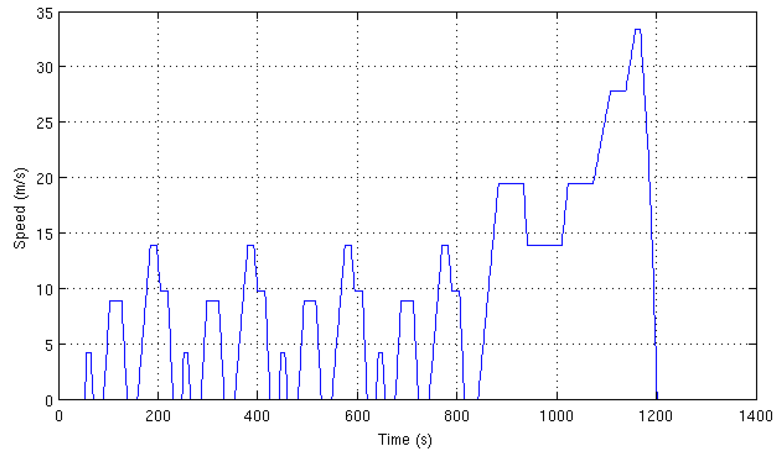
2. Drivecycles Employed

| Parameters | NEDC | Real-World | Artemis |
|---|---|---|---|
| Distance | 10.93 km | 29.83 km | 73.02 km |
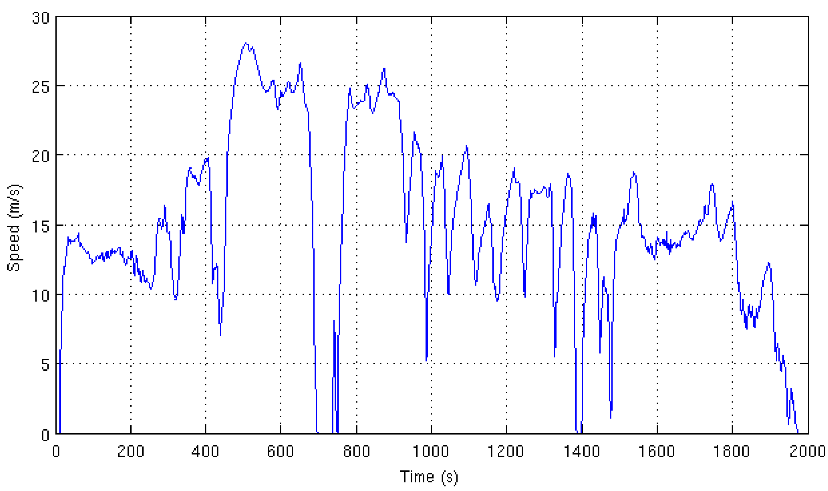
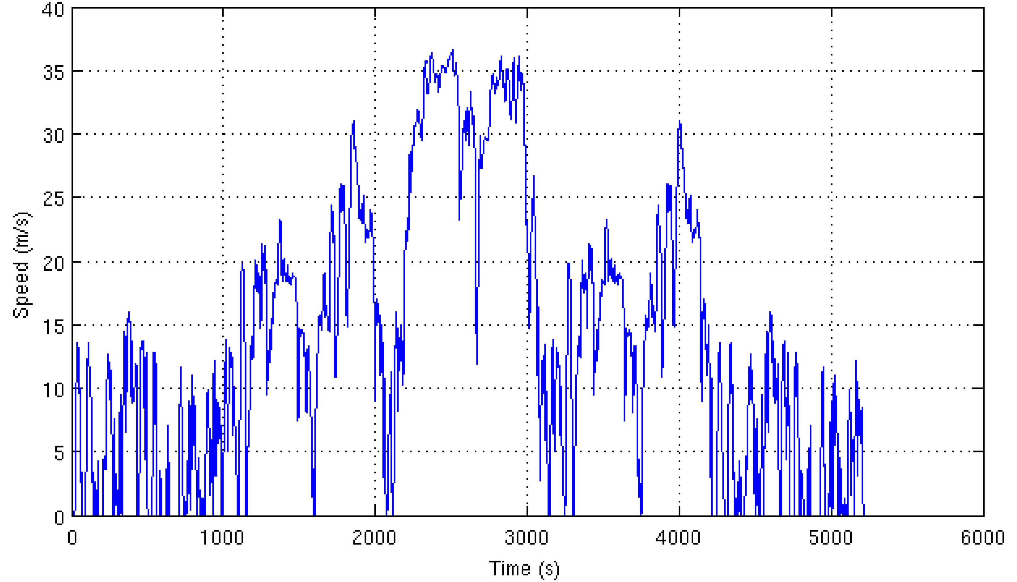
| Top Speed | 33.33 m/s | 28.04 m/s | 36.60 m/s |
| Maximum Acceleration | 1.04 m/s2 | 3.23 m/s2 | 2.86 m/s2 |
| Number of repetitions | 10 | 7 | 2 |
| Total distance covered | 109.32 km | 208.81 km | 146.04 km |
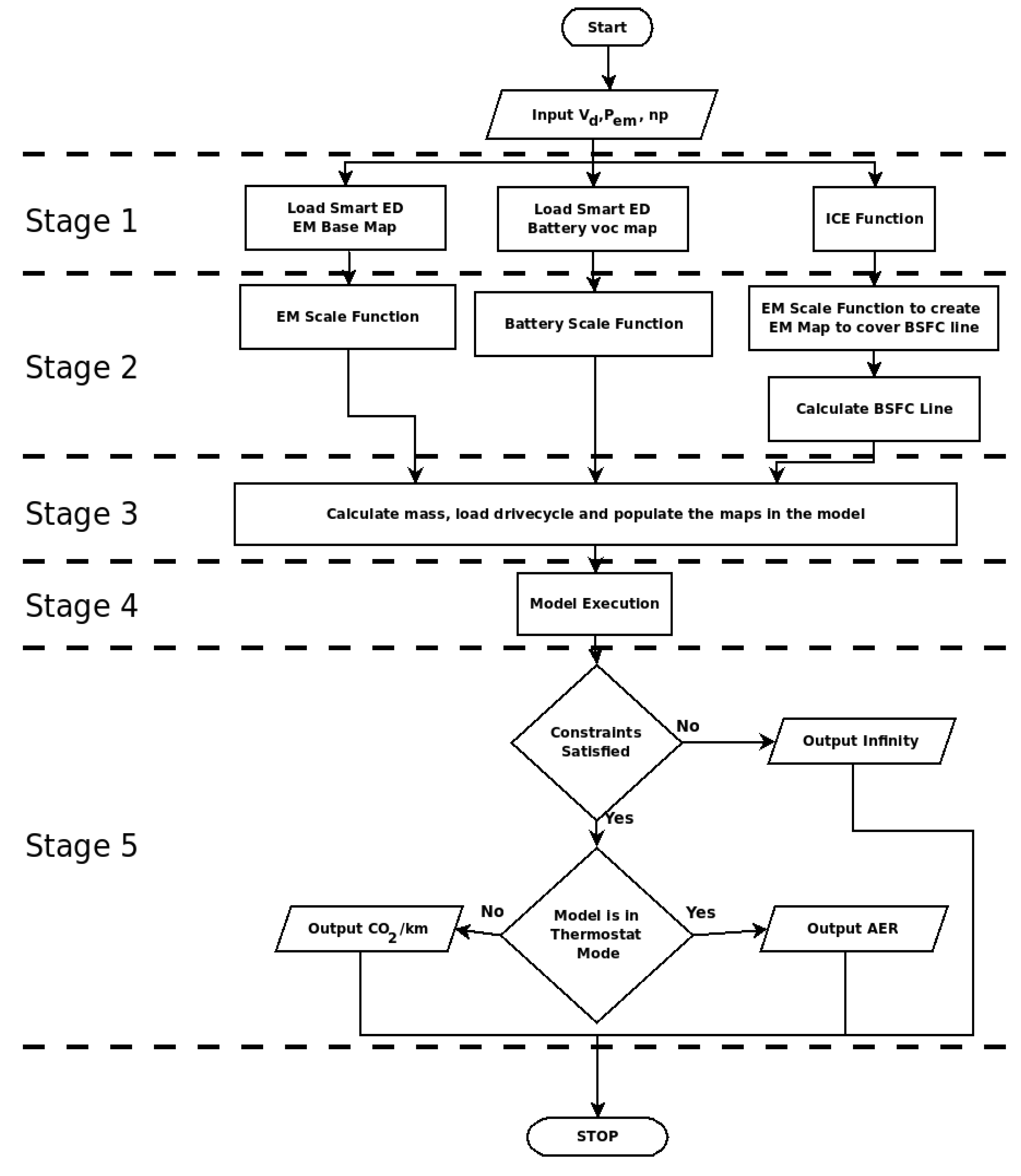
3. Design of a Scalable PHEV Model to Support System Optimization
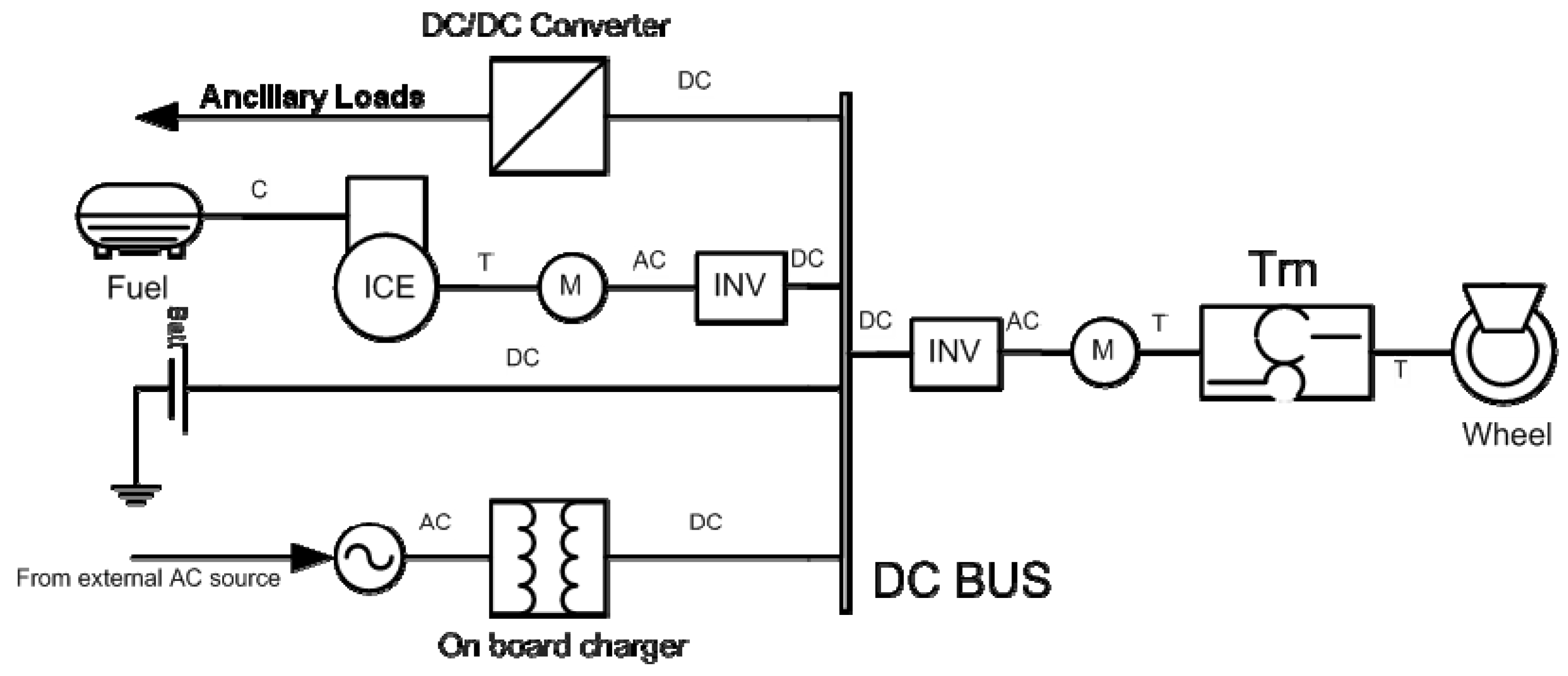
3.1. Vehicle Model
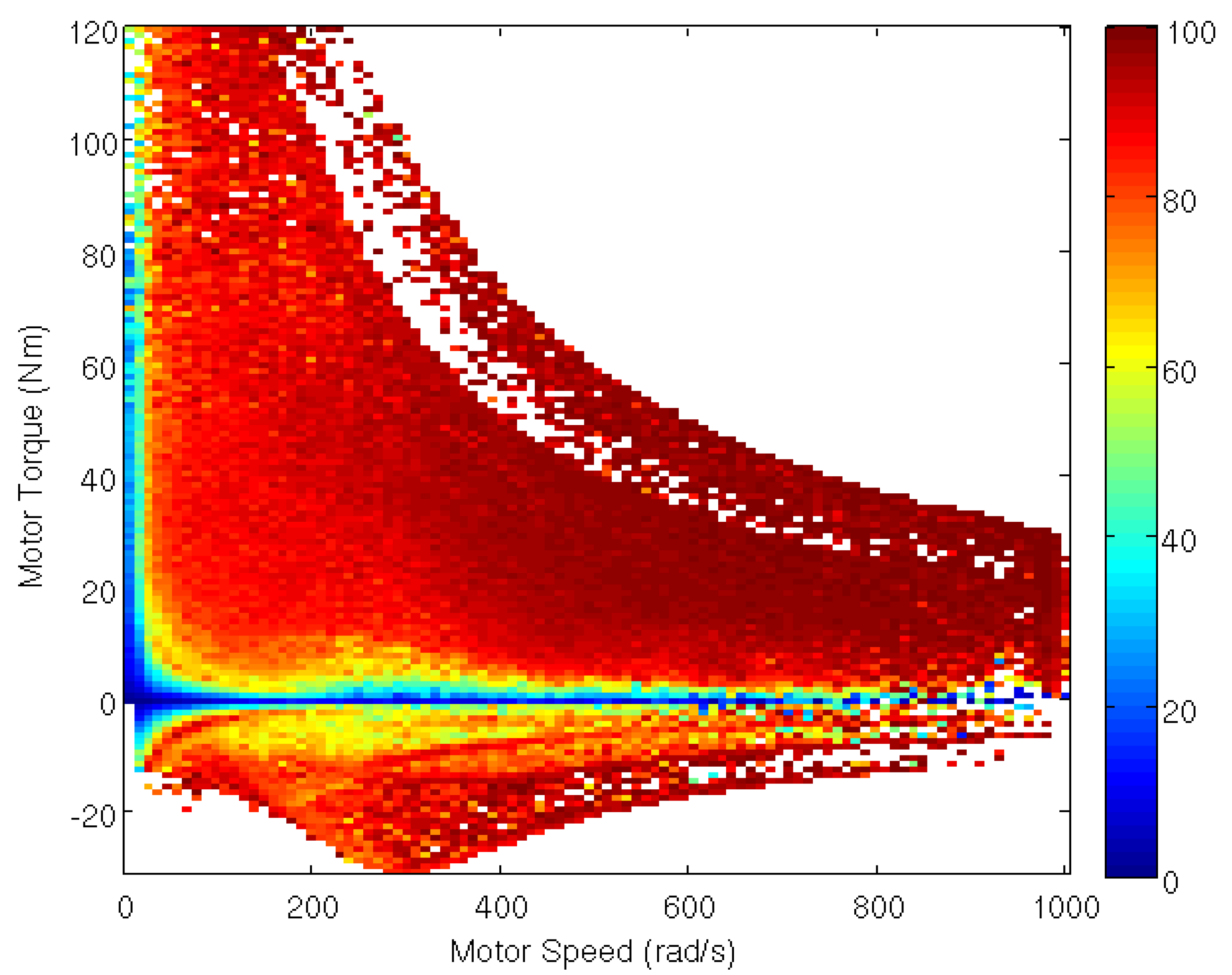
3.2. Integrated Electric Machine and Transmission
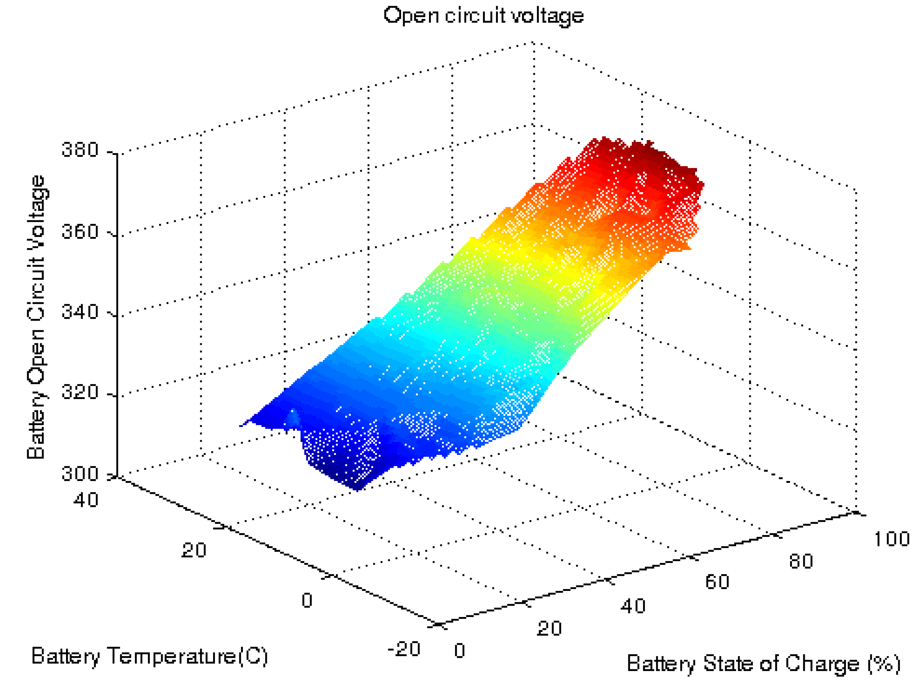
3.3. Battery Model

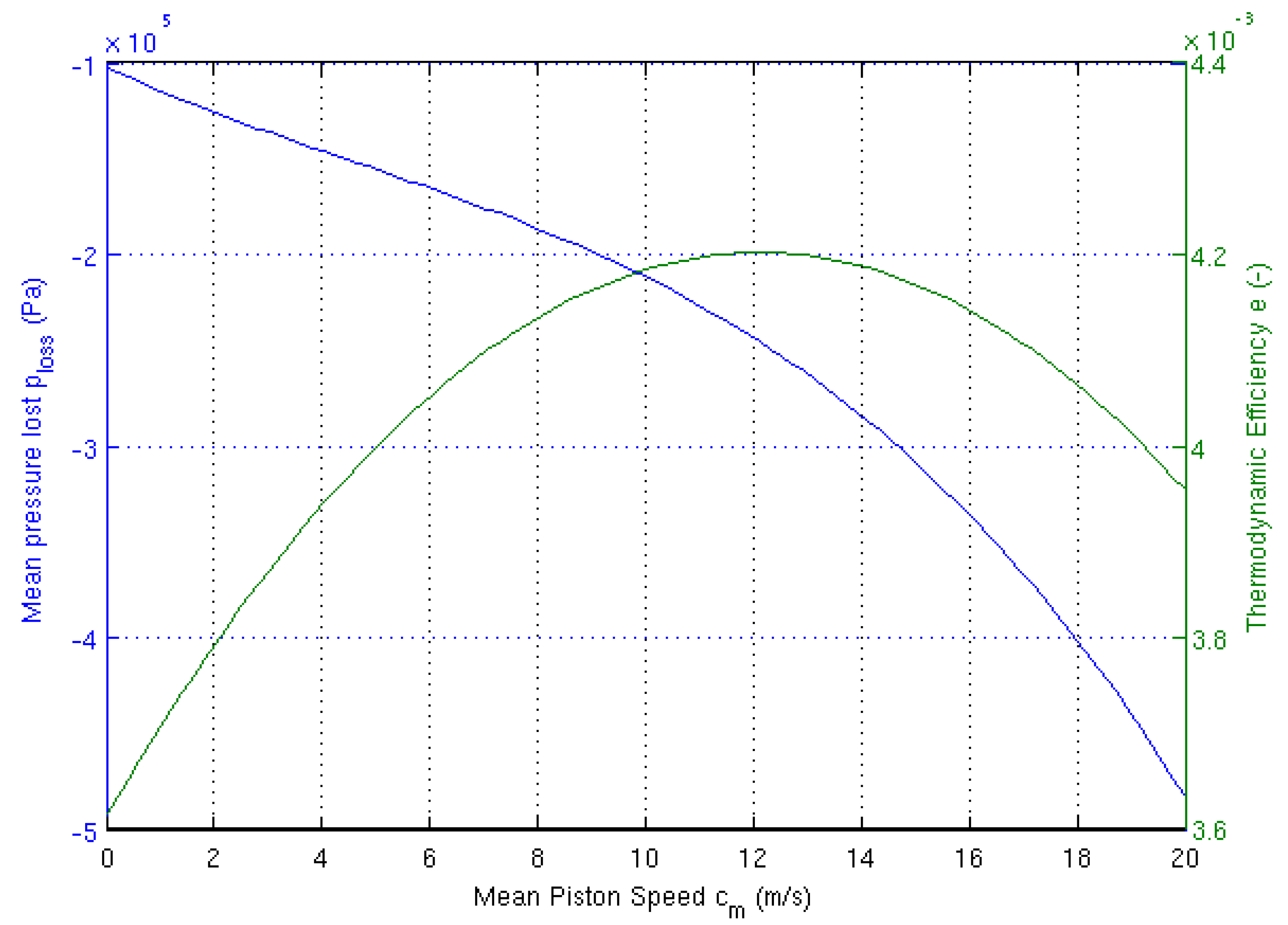
3.4. Integrated ICE and Generator
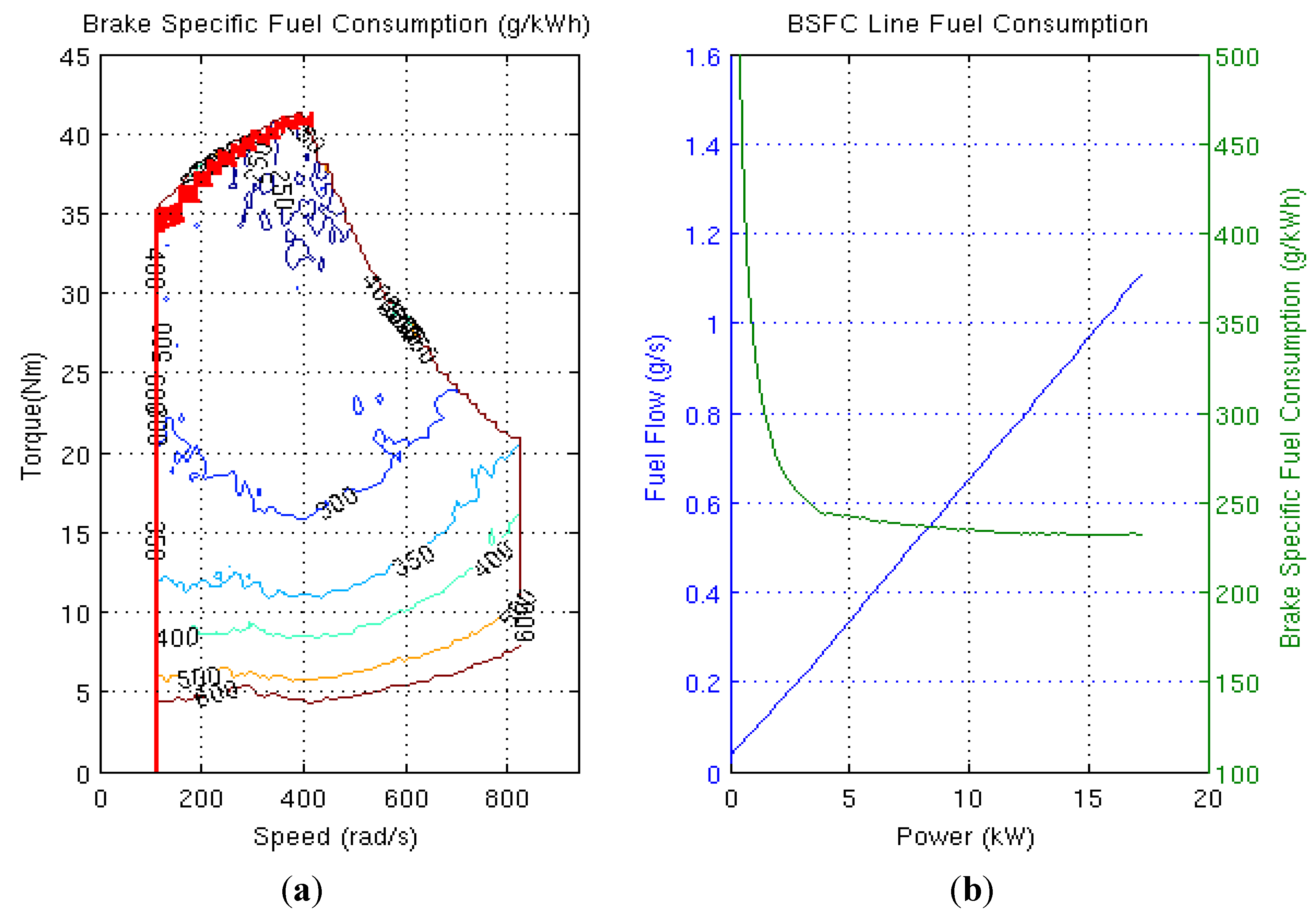
3.4.1. Creation of Engine Efficiency and Fuel Consumption Map
3.4.2. Identification of best operating line
3.5. Financial Cost Model
4. Energy Management Control Strategy
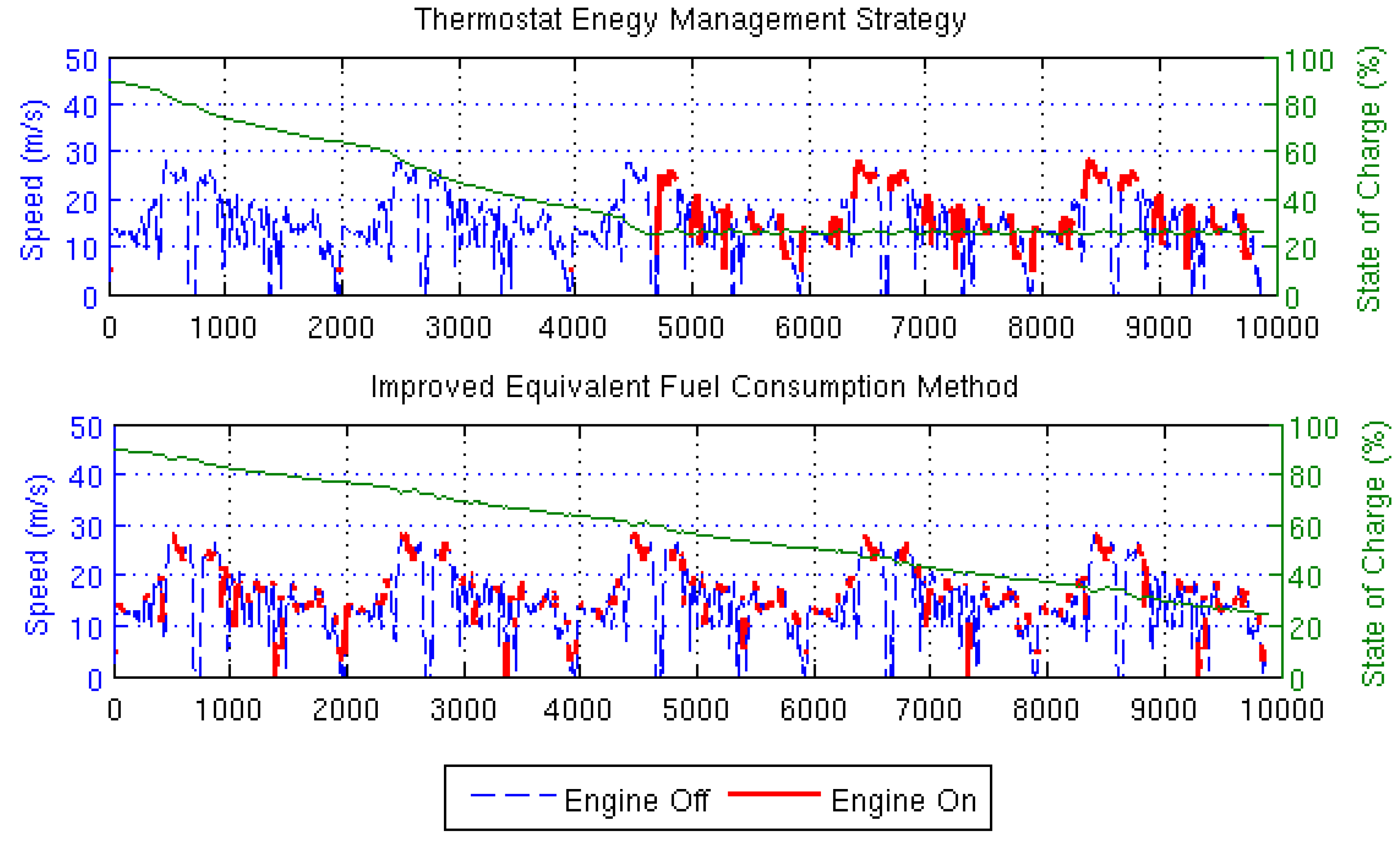
4.1. Thermostat/Heuristic Rule-based Control Strategy
if (SoC< LOWER TRESHOLD) Engine is switched on else if (SoC> UPPER THRESHOLD) Engine is switched off else if (P_dmd>P_bat(max)) Engine is switched on else Repeat previous state end if (P_eng_best>P_bat +P_dmd) P_eng = P_bat + P_dmd else if (P_eng_best<P_dmd - P_bat) P_eng = P_dmd – P_bat else P_eng = P-eng_best end |
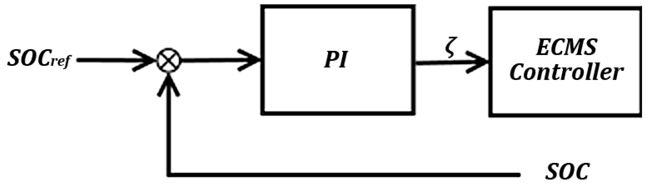
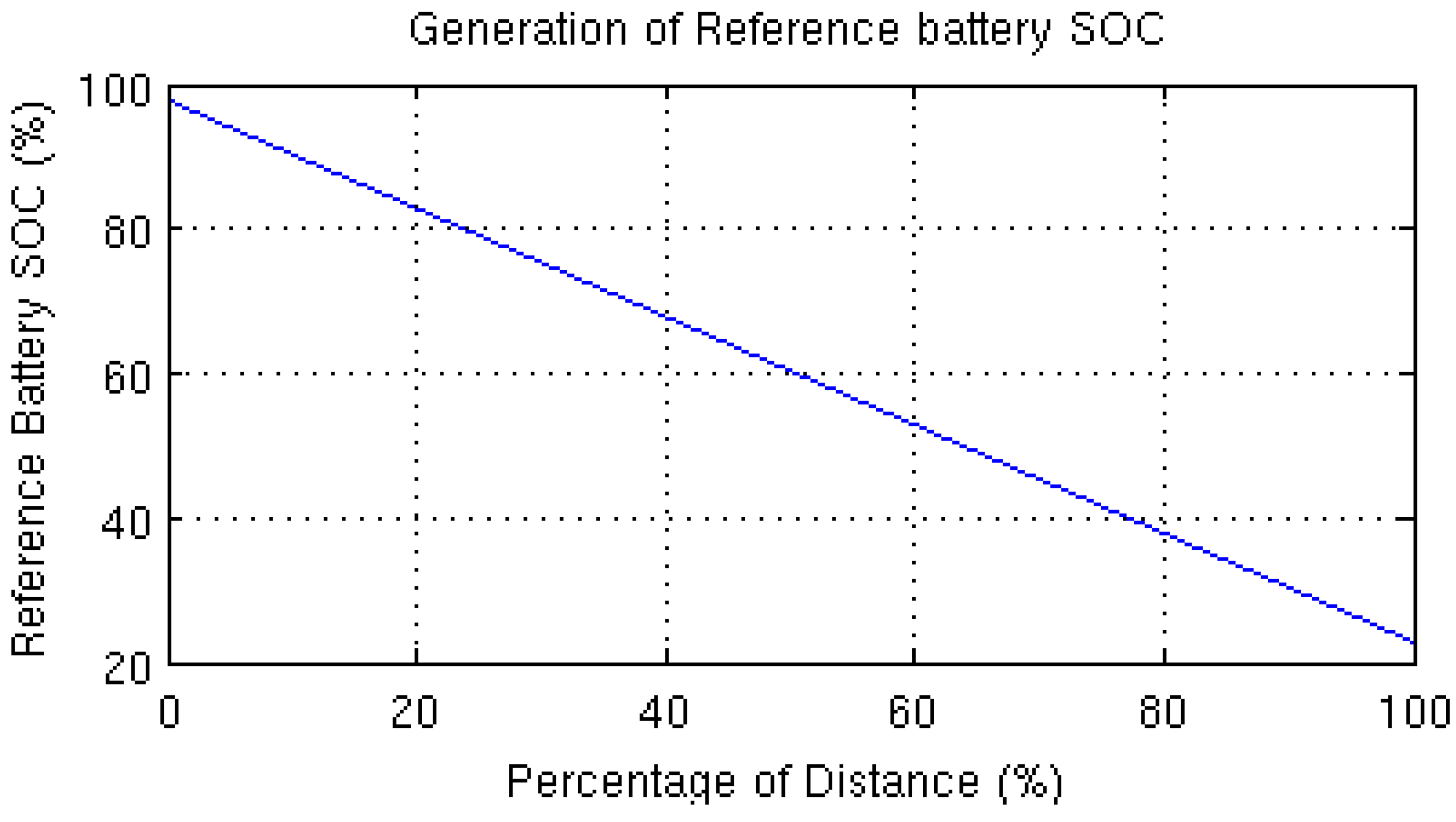
4.2. Improved Equivalent Consumption Minimization Strategy (ECMS)


4.3. Control System Comparison

5. Component Sizing
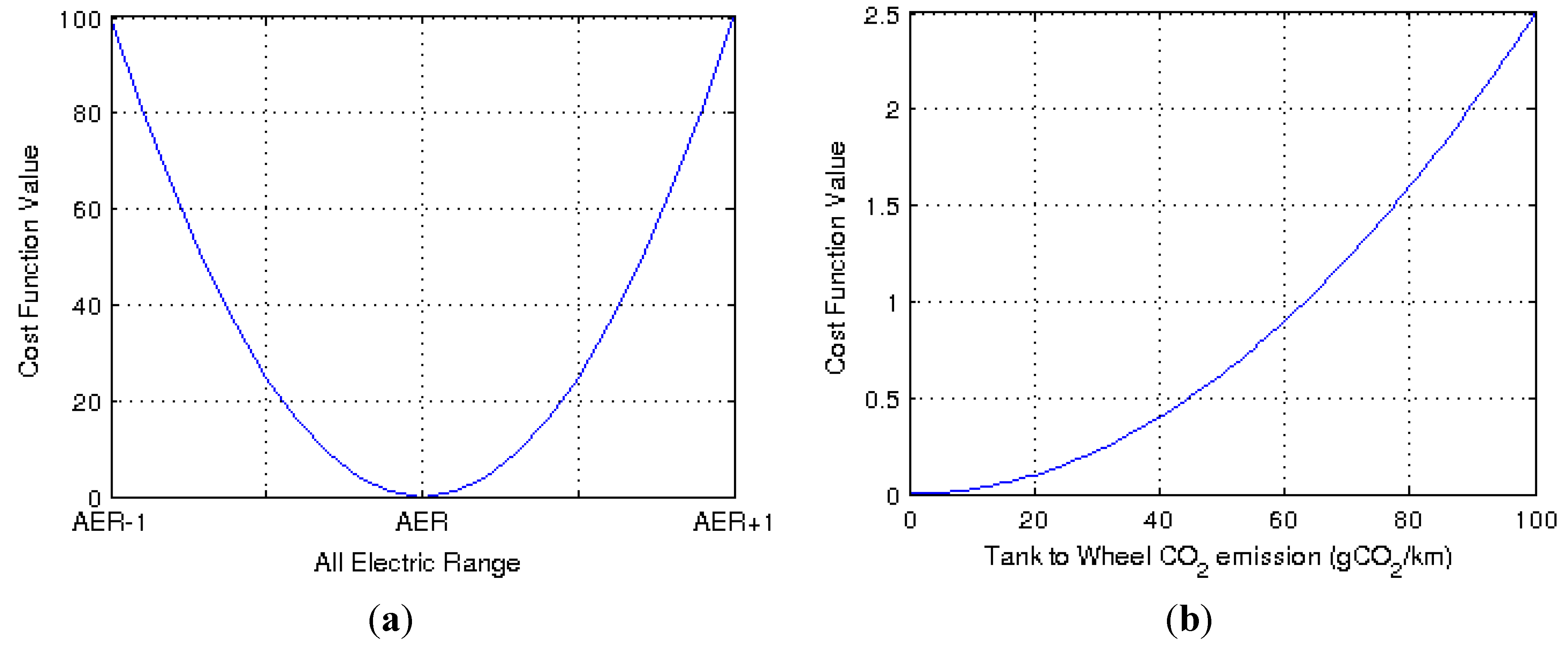
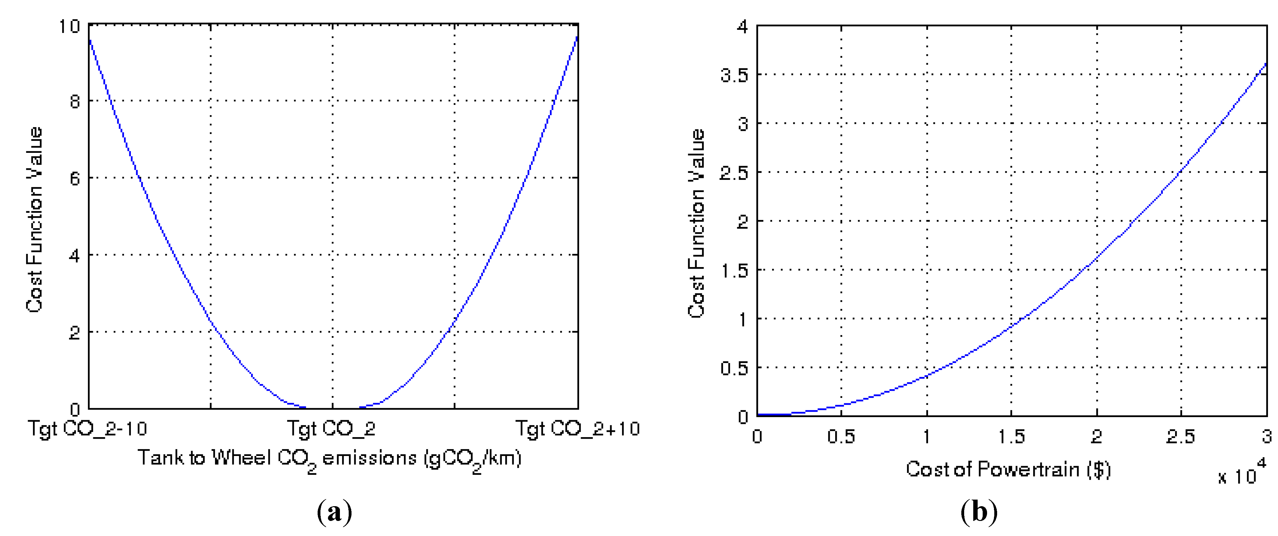
5.1. The Optimization Algorithm
5.2. The Optimization Framework
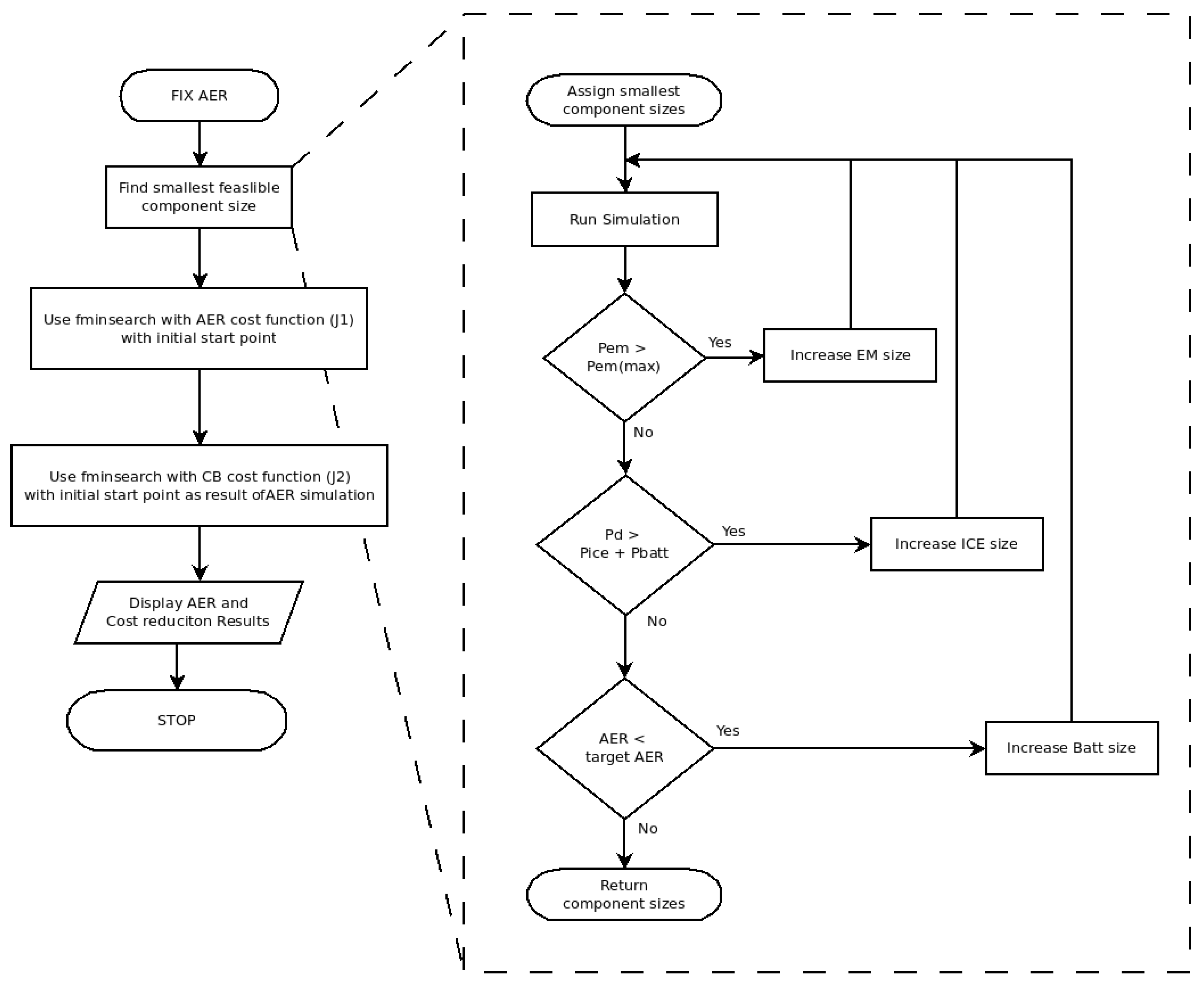
- Engine volumetric size (Vd);
- Electric machine power (Pem(peak));
- Battery number of strings in parallel (np);
- Upper threshold calibration for the thermostat controller.


6. Results
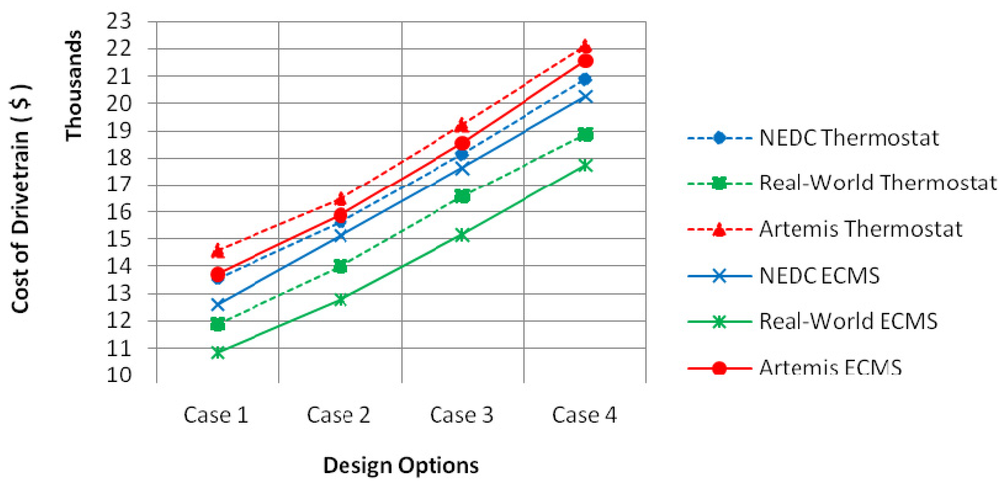
6.1. PHEV Powertrain Cost Reduction
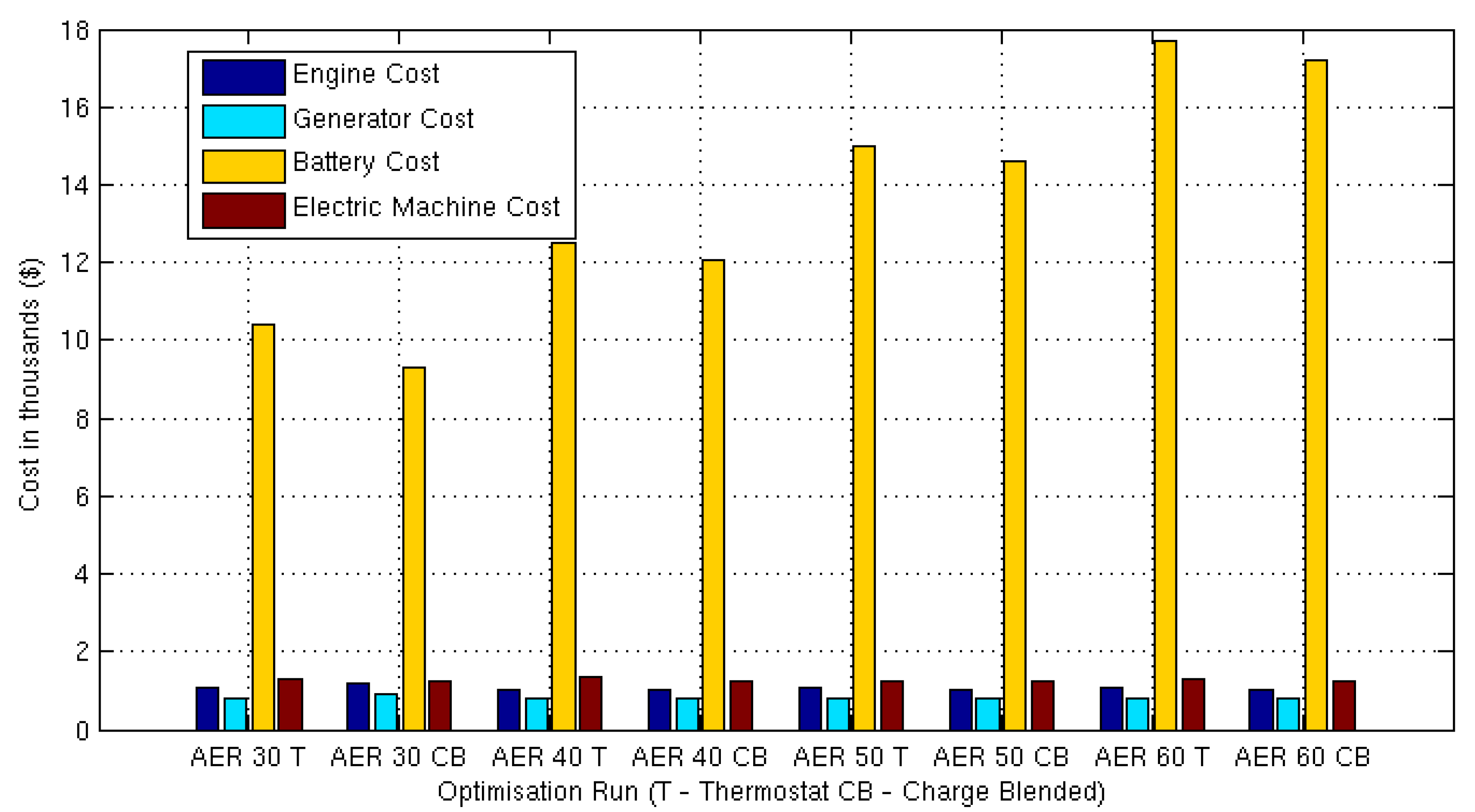
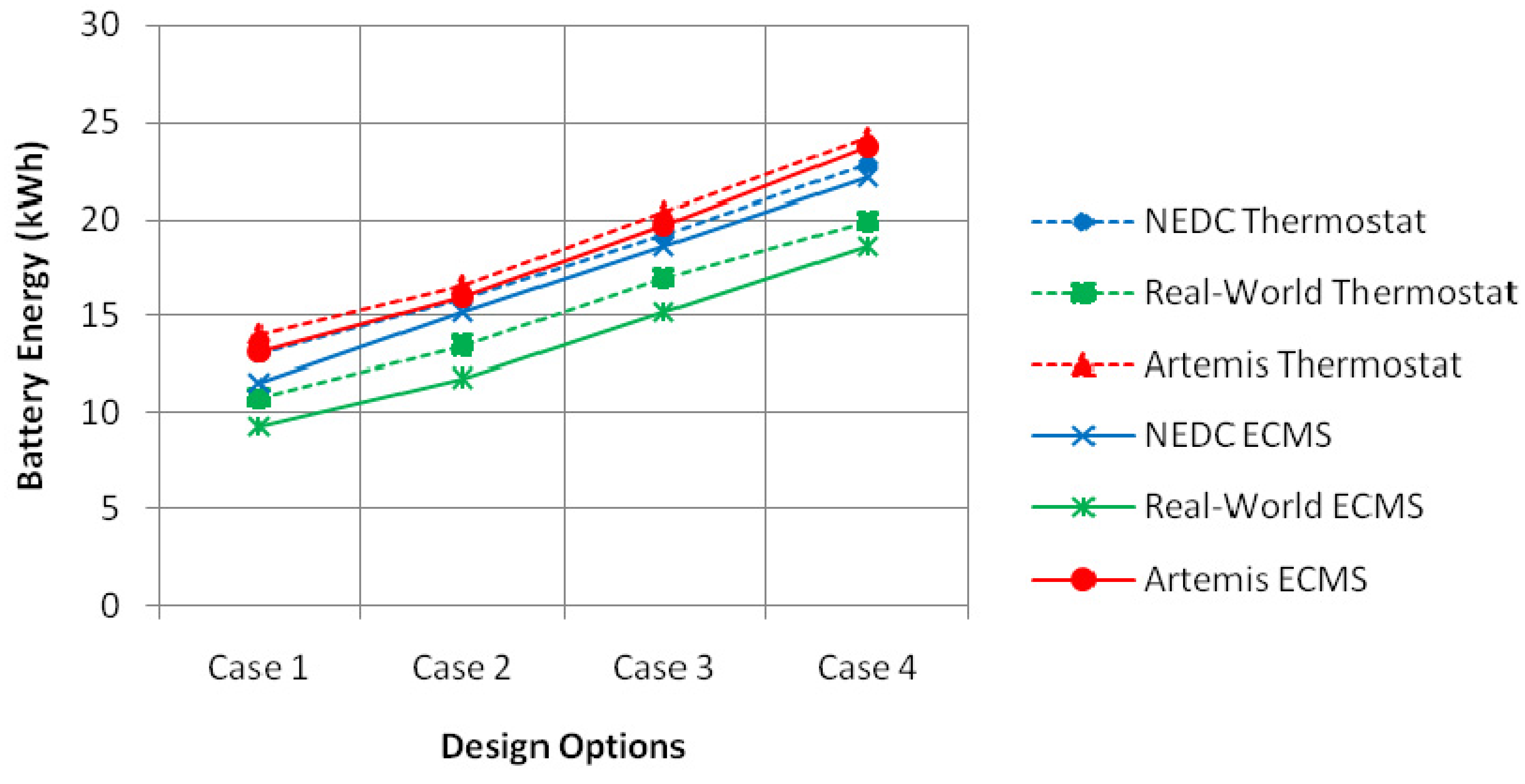
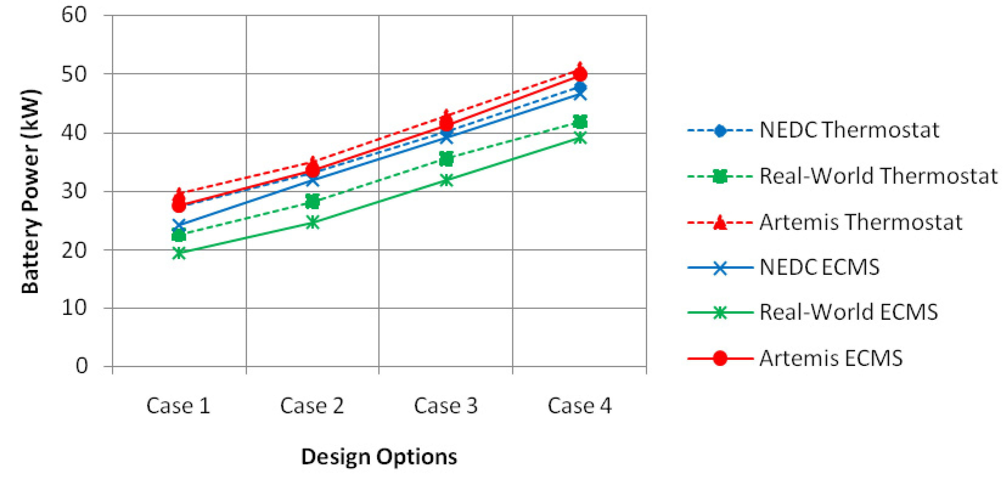
6.2. Downsizing of the HV Battery


| Drivecycle: NEDC | |||||||||||||
| Parameters | Design Case 1 | Design Case 2 | Design Case 3 | Design Case 4 | |||||||||
| Thermostat | Improved ECMS | Change | Thermostat | Improved ECMS | Change | Thermostat | Improved ECMS | Change | Thermostat | Improved ECMS | Change | ||
| AER (km) | 48 | 64 | 80 | 96 | |||||||||
| Vd (mL) | 538.13 | 650.28 | 21% | 507.82 | 531.90 | 5% | 541.43 | 500.06 | −8% | 537.36 | 500.01 | −7% | |
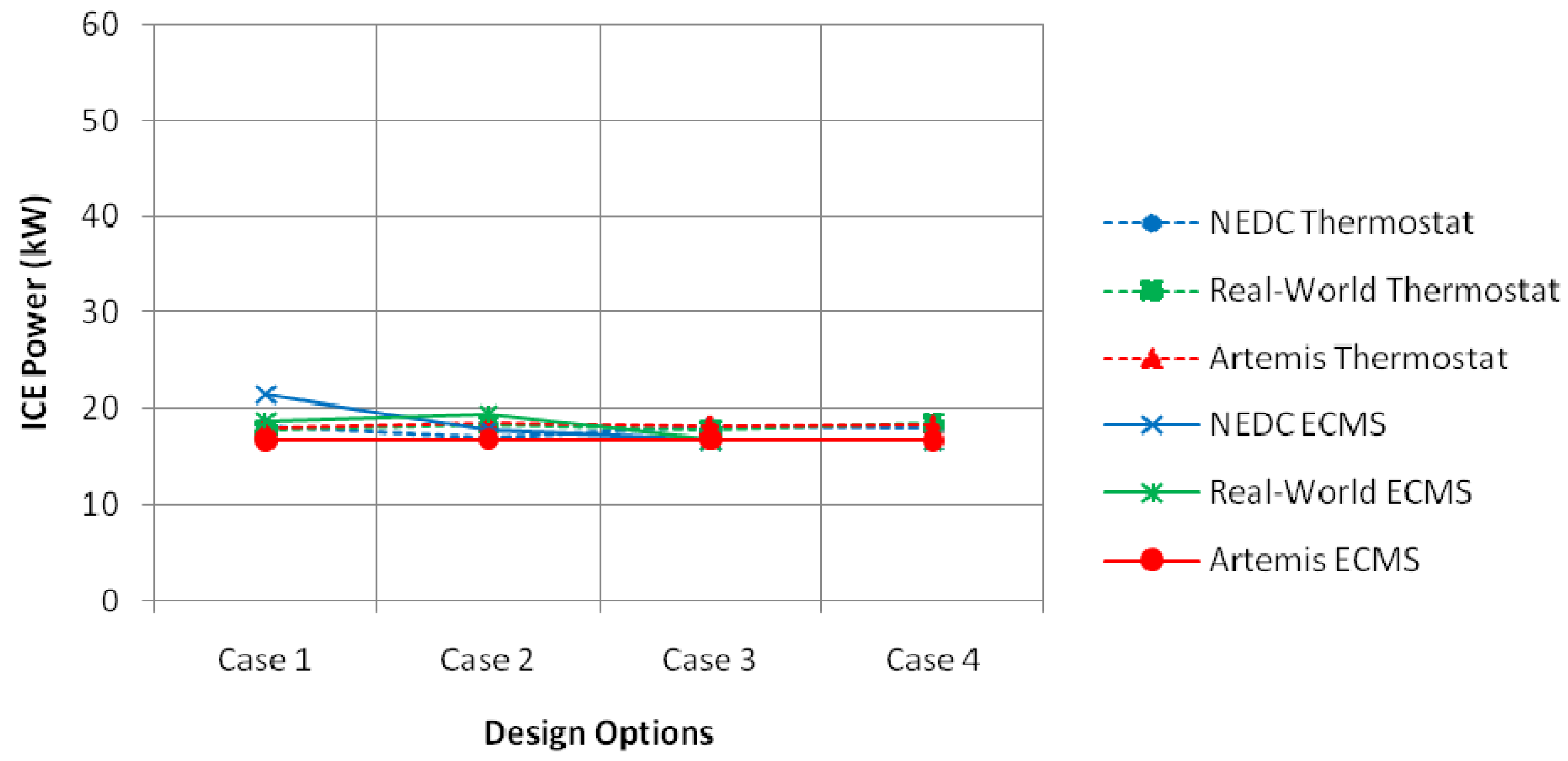
| Pice (kW) | 18.02 | 21.54 | 20% | 16.98 | 17.79 | 5% | 18.14 | 16.75 | −8% | 17.99 | 16.75 | −7% | |
| Pem (kW) | 38.95 | 36.50 | −6% | 41.52 | 36.80 | −11% | 38.88 | 37.35 | −4% | 40.49 | 37.30 | −8% | |
| Pbat (kW) | 27.32 | 24.33 | −11% | 33.21 | 31.95 | −4% | 40.19 | 39.12 | −3% | 47.88 | 46.51 | −3% | |
| Qbat (kWh) | 13.02 | 11.59 | −11% | 15.82 | 15.22 | −4% | 19.15 | 18.64 | −3% | 22.81 | 22.16 | −3% | |
| TTW (g CO2/km) | 69.99 | 70.51 | 1% | 54.68 | 55.26 | 1% | 39.62 | 40.12 | 1% | 23.29 | 23.61 | 1% | |
| Cost ($) | 13,538.67 | 12,607.44 | −7% | 15,635.85 | 15,126.79 | −3% | 18,118.63 | 17,633.27 | −3% | 20,877.84 | 20,260.40 | −3% | |
| Drivecycle: Real−World | |||||||||||||
| Parameters | Design Case 1 | Design Case 2 | Design Case 3 | Design Case 4 | |||||||||
| Thermostat | Improved ECMS | Change | Thermostat | Improved ECMS | Change | Thermostat | Improved ECMS | Change | Thermostat | Improved ECMS | Change | ||
| AER (km) | 48 | 64 | 80 | 96 | |||||||||
| Vd (mL) | 528.00 | 562.91 | 7% | 546.26 | 584.83 | 7% | 532.27 | 500.57 | −6% | 554.58 | 500.42 | −10% | |
| Pice (kW) | 17.65 | 18.66 | 6% | 18.32 | 19.39 | 6% | 17.81 | 16.77 | −6% | 18.44 | 16.76 | −9% | |
| Pem (kW) | 41.17 | 40.74 | −1% | 44.05 | 42.35 | −4% | 44.95 | 41.82 | −7% | 46.06 | 43.05 | −7% | |
| Pbat (kW) | 22.60 | 19.53 | −14% | 28.24 | 24.75 | −12% | 35.53 | 31.84 | −10% | 41.77 | 39.08 | −6% | |
| Qbat (kWh) | 10.77 | 9.30 | −14% | 13.46 | 11.79 | −12% | 16.93 | 15.17 | −10% | 19.90 | 18.62 | −6% | |
| TTW (g CO2/km) | 83.17 | 83.61 | 1% | 77.23 | 77.82 | 1% | 68.40 | 68.98 | 1% | 59.97 | 60.55 | 1% | |
| Cost ($) | 11,890.76 | 10,846.26 | −9% | 13,990.67 | 12,776.07 | −9% | 16,578.49 | 15,143.13 | −9% | 18,856.06 | 17,744.06 | −6% | |
| Drivecycle: Artemis | |||||||||||||
| Parameters | Design Case 1 | Design Case 2 | Design Case 3 | Design Case 4 | |||||||||
| Thermostat | Improved ECMS | Change | Thermostat | Improved ECMS | Change | Thermostat | Improved ECMS | Change | Thermostat | Improved ECMS | Change | ||
| AER (km) | 48 | 64 | 80 | 96 | |||||||||
| Vd (mL) | 534.05 | 500.02 | −6% | 553.96 | 501.71 | −9% | 539.05 | 501.35 | −7% | 545.27 | 500.12 | −8% | |
| Pice (kW) | 17.87 | 16.75 | −6% | 18.49 | 16.81 | −9% | 18.06 | 16.79 | −7% | 18.28 | 16.75 | −8% | |
| Pem (kW) | 50.59 | 45.24 | −11% | 50.00 | 46.58 | −7% | 46.77 | 43.39 | −7% | 48.94 | 44.25 | −10% | |
| Pbat (kW) | 29.52 | 27.62 | −6% | 34.87 | 33.57 | −4% | 42.79 | 41.33 | −3% | 50.81 | 49.77 | −2% | |
| Qbat (kWh) | 14.07 | 13.16 | −6% | 16.61 | 15.99 | −4% | 20.39 | 19.69 | −3% | 24.21 | 23.71 | −2% | |
| TTW (g CO2/km) | 81.98 | 83.37 | 2% | 71.48 | 72.99 | 2% | 57.60 | 59.17 | 3% | 43.54 | 45.10 | 4% | |
| Cost ($) | 14,565.78 | 13,716.97 | −6% | 16,486.78 | 15,863.46 | −4% | 19,210.74 | 18,554.40 | −3% | 22,117.47 | 21,570.86 | −2% | |
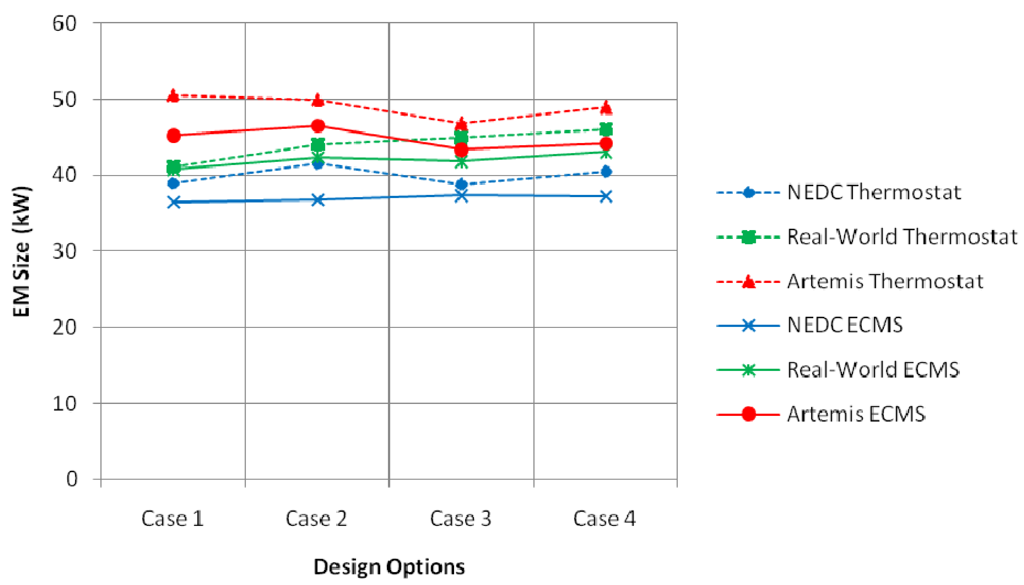
6.3. Optimization of the Electrical Machine and ICE

7. Discussion
7.1. PHEV Model
7.2. Energy Management Control System
7.3. Optimization Framework and Component Scaling
8. Conclusions
Abbreviations
| AER | All Electric Range |
| APU | Auxiliary Power Unit |
| Batt | Battery |
| BSFC | Brake Specific Fuel Consumption |
| CAN | Controller Area Network |
| CB | Charge Blending |
| CD | Charge Depleting |
| CO2 | Carbon Dioxide |
| CS | Charge Sustaining |
| DOT | Department of Transport |
| DOD | Depth of Discharge |
| DP | Dynamic Programming |
| ECMS | Equivalent Consumption Minimization Strategy |
| EOL | End of Life |
| EPA | Environment Protection Agency |
| EU | European Union |
| EV | Electric Vehicle |
| GPS | Global Positioning System |
| HEV | Hybrid Electric Vehicle |
| HV | High Voltage |
| ICE | Internal Combustion Engine |
| INV | Inverter |
| NEDC | New European Driving Cycle |
| NN | Neural Network |
| PHEV | Plug-in Hybrid Electric Vehicle |
| PI | Proportional plus Integral Controller |
| PSAT | Powertrain Systems Analysis Toolkit |
| SoC | State of Charge |
| SoCinit | Initial State of Charge |
| Trn | Transmission |
| UNECE | United Nations Economic Commission for Europe |
| US | United States |
Notations
Total resistive force on the tyre (N) | |
Lower heating value of fuel (J/kg) | |
Total mass of the vehicle (kg) | |
Number of strokes per cycle (-) | |
Power drawn by the ancillaries (W) | |
Power provided by the battery (W) | |
Peak power of the battery (W) | |
Power demand (W) | |
Peak power of the electric machine (W) | |
Power drawn by the electric machine (W) | |
Scaled peak power of the electric machine (W) | |
Peak power of internal combustion engine (W) | |
Power provided by the ICE (W) | |
Capacity of the battery (Ah) | |
Capacity of the individual cell (Ah) | |
Resistance of the battery pack (Ω) | |
Resistance of an individual cell (Ω) | |
Internal Resistance of the battery (Ω) | |
Torque of the engine (Nm) | |
Torque of the electric machine (Nm) | |
Torque of the base electric machine map (Nm) | |
Scaled torque of the electric machine (Nm) | |
Torque at the wheels (Nm) | |
Volumetric size of the engine (m3) | |
Mean piston speed (m/s) | |
Final drive gear ratioratio(-) | |
Battery current (A) | |
Mass of fuel (kg) | |
Mass of the chassis (kg) | |
Mass of the battery (kg) | |
Mass of electrical machine (kg) | |
Mass of the ICE (kg) | |
Mechanical loss in terms of pressure (Pa) | |
Mean effective pressure (Pa) | |
Mean fuel pressure (Pa) | |
Radius of the wheel (m) | |
Open circuit voltage of the battery pack | |
Open circuit voltage of an individual cell | |
Terminal voltage at the battery (V) | |
Efficiency of the engine (-) | |
Efficiency of the electric machine (-) | |
Engine speed (rad/s) | |
Speed of the electric machine (rad/s) | |
Stroke length (m) | |
Thermodynamic efficiency (-) | |
Acceleration due to gravity (9.81 m/s2) | |
Number of parallel strings | |
Number of cells in series | |
Vehicle velocity (km/h) | |
Slope of the road (-) | |
Power split ratio | |
Equivalence ratio for battery fuel consumption (-) |
Acknowledgements
Appendix
A1. Drivecycles


A2. Trial Programme
| Trial program parameters | Data |
|---|---|
| Duration of Program | November 2010–March 2011 |
| Number of vehicles | 8 |
| Types of Vehicles | 7 Smart EVs and 1 Mitsubishi i-Miev |
| Total kilometers driven by Smart EVs during program | 4268 km |
| Number of demonstration days | 12 |
| Number of participating organizations | 5 |
| Vehicle Parameter | Unit | Description |
|---|---|---|
| Battery voltage | V | Terminal voltage of the HV battery |
| Battery current | A | Battery current measured at the terminals of the battery pack |
| Machine speed | Rad/s | Rotational velocity of the electrical machine |
| Machine voltage | V | DC voltage, measured at the input to the inverter |
| Machine current | A | Machine current measured at the terminals of the inverter |
| Auxiliary power | kW | Power consumed by ancillary devices, including power steering and thermal management of the cabin and battery pack |
| Charger voltage | V | AC mains voltage measured by the onboard charger |
| Charger current | A | AC Mains current measured by the onboard charger |
| Battery temperature | °C | Individual measurement of battery pack temperature |
References
- Chan, C.C. The state of the art of electric, hybrid, and fuel cell vehicles. Proc. IEEE 2007, 95, 704–718. [Google Scholar] [CrossRef]
- Douglas, C.; Stewart, A. Influences on the Low Carbon Car Market from 2020–2030; Final Report 2011; Report for Low Carbon Vehicle Partnership: Cambridge, UK, 2011. [Google Scholar]
- Franke, T.; Neumann, I.; Bühler, F.; Cocron, P.; Krems, J.F. Experiencing range in an electric vehicle: Understanding psychological barriers. Appl. Psychol. 2012, 61, 368–391. [Google Scholar] [CrossRef]
- Markel, T.; Simpson, A. Plug-In Hybrid Electric Vehicle Energy Storage System Design. In Proceedings of the Advanced Automotive Battery Conference, Baltimore, MD, USA, 17–19 May 2006; pp. 1–9.
- Patil, R.; Adornato, B.; Filipi, Z. Impact of Naturalistic Driving Patterns on PHEV Performance and System Design. In Proceedings of the SAE 2009 Powertrains Fuels and Lubricants Meeting, San Antonio, TX, USA, 2 November 2009. SAE Technical Paper 2009-01-2715.
- Shiau, C.N.; Samaras, C.; Hauffe, R.; Michalek, J.J. Impact of battery weight and charging patterns on the economic and environmental benefits of plug-in hybrid vehicles. Energy Policy 2009, 37, 2653–2663. [Google Scholar] [CrossRef]
- Kammen, D.M.; Arons, S.M.; Lemoine, D.; Hummel, H. Cost-Effectiveness of Greenhouse Gas Emission Reductions from Plug-in Hybrid Electric Vehicles; Working Paper No. GSPP08-014; Goldman School of Public Policy: Berkeley, CA, USA, 2008. [Google Scholar]
- Moura, S.J.; Callaway, D.S.; Fathy, H.K.; Stein, J.L. Impact of battery sizing on stochastic optimal power management in plug-in hybrid electric vehicles. In Proceedings of the IEEE International Conference on Vehicular Electronics and Safety, Columbus, OH, USA, 22–24 September 2008; pp. 96–102.
- Tulpule, P.; Marano, V.; Rizzoni, G. Effects of different PHEV Control Strategies on Vehicle Performance. In Proceedings of the American Control Conference, St. Louis, MO, USA, 10 June 2009; pp. 3950–3955.
- Karbowski, D. Impact of Component Size on Plug-In Hybrid Vehicle Energy Consumption Using Global Optimization. In Proceedings of the 23rd International Electric Vehicle Symposium (EVS23), Anaheim, CA, USA, 2 December 2007.
- Shankar, R.; Marco, J.; Assadian, F. Design of an Optimized Charge-Blended Energy Management Strategy for a Plug-in Hybrid Vehicle. In Proceedings of the UKACC (United Kingdom Automatic Control Council) International Conference on Control, Cardiff, UK, 3–5 September 2012; pp. 1–6.
- Dextreit, C.; Assadian, F.; Kolmanovsky, I.; Mahtani, J.; Burnham, K. Hybrid Electric Vehicle Energy Management Using Game Theory. In Proceedings of the SAE World Congress & Exhibition, Detroit, MI, USA, 14 April 2008. SAE Technical Paper 2008-01-1317.
- Shankar, R.; Marco, J.; Assadian, F. A methodology to Determine Drivetrain Efficiency Based on External Environment. In Proceedings of the IEEE International Electric Vehicle Conference (IEVC), Greenville, SC, USA, 4–8 March 2012; pp. 1–6.
- Smart Electric Drive Homepage. Available online: http://uk.smart.com/ (accessed on 16 November 2011).
- Wu, X.; Cao, B.; Li, X.; Xu, J.; Ren, X. Component sizing optimization of plug-in hybrid electric vehicles. Appl. Energy 2011, 88, 799–804. [Google Scholar] [CrossRef]
- Zytek IDT 120-55 Integrated 55 kW Electric Engine. Available online: http://www.zytekautomotive.co.uk/Products/ElectricEngines/55kW.aspx (accessed on 16 November 2012).
- Tremblay, O.; Dessaint, L.; Dekkiche, A. A Generic Battery Model for the Dynamic Simulation of Hybrid Electric Vehicles. In Proceedings of the IEEE Vehicle Power and Propulsion Conference, Arlington, TX, USA, 9 September 2007.
- Rizzoni, G.; Guzzella, L.; Baumann, B.M. Unified modeling of hybrid electric vehicle drivetrains. Mechatronics 1999, 4, 246–257. [Google Scholar] [CrossRef]
- Guzzella, L.; Sciarretta, A. Vehicle Propulsiton Systems: Introduction to Modeling and Optmization; Springer-Verlag: Berlin, Germany, 2005. [Google Scholar]
- Silva, C.; Ross, M.; Farias, T. Evaluation of energy consumption, emissions and cost of plug-in hybrid vehicles. Energy Convers. Manag. 2009, 50, 1635–1643. [Google Scholar] [CrossRef]
- Simpson, A. Cost-Benefit Analysis of Plug-in Hybrid Electric Vehicle Technology. In Proceedings of the 22nd International Battery, Hybrid and Fuel Cell Electric Vehicle Symposium and Exhibition (EVS-22), Yokohama, Japan, 23 October 2006.
- O’Keefe, M.; Brooker, A.; Johnson, C.; Mendelsohn, M.; Neubauer, J. Battery Ownership Model: A Tool for Evaluating the Economics of Electrified Vehicles and Related Infrastructure. In Proceedings of the 25th International Battery, Hybrid and Fuel Cell Electric Vehicle Symposium and Exposition, Shenzhen, China, 5 November 2010.
- Paganelli, G.; Guerra, T.M.; Delprat, S.; Santin, J.J.; Delhom, M.; Combes, E. Simulation and assessment of power control strategies for a parallel hybrid car. J. Automob. Eng. 2000, 214, 705–717. [Google Scholar] [CrossRef]
- Serrao, L.; Onori, S.; Rizzoni, G. ECMS as a realization of Pontryagin’s minimum principle for HEV control. In Proceedings of the IEEE American Control Conference, St. Louis, MO, USA, 10 June 2009; pp. 3964–3969.
- Zhang, C.; Vahidi, A.; Pisu, P.; Li, X.; Tennent, K. Role of terrain preview in energy management of hybrid electric vehicles. IEEE Trans. Veh. Tech. 2009, 59, 1139–1147. [Google Scholar]
- Pisu, P.; Rizzoni, G. A comparative study of supervisory control strategies for hybrid electric vehicles. IEEE Trans. Control Syst. Tech. 2007, 15, 506–518. [Google Scholar] [CrossRef]
- Musardo, C.; Rizzoni, G.; Staccia, B. A-ECMS: An Adaptive Algorithm for Hybrid Electric Vehicle Energy Management. In Proceedings of 44th IEEE Conference on Decision and Control, Seville, Spain, 12December 2005; pp. 1816–1823.
- Stamps, A.T.; Holland, C.E.; White, R.E.; Gatzke, E.P. Analysis of capacity fade in a lithium ion battery. J. Power Sources 2005, 150, 229–239. [Google Scholar] [CrossRef]
- Kai, L.C.; Li, P.Y.; Chase, T.R. Optimal Design of Power-Split Transmissions for Hydraulic Hybrid Passenger Vehicles. In Proceedings of the IEEE American Control Conference (ACC), San Francisco, CA, USA, 29 June 2011; pp. 3295–3300.
- Lagarias, J.; Reeds, J.; Wright, M.; Wright, P. Convergence properties of the Nelder–Mead simplex method in low dimensions. SIAM J. Optim. 1998, 9, 112–147. [Google Scholar] [CrossRef]
- Liaw, B.Y.; Dubarry, M. From driving cycle analysis to understanding battery performance in real-life electric hybrid vehicle operation. J. Power Sources 2007, 174, 76–88. [Google Scholar] [CrossRef]
- Smith, K.; Wang, C. Power and thermal characterization of a lithium-ion battery pack for hybrid-electric vehicles. J. Power Sources 2006, 160, 662–673. [Google Scholar] [CrossRef]
- Alkidas, A.C. Combustion advancements in gasoline engines. Energy Convers. Manag. 2007, 48, 2751–2761. [Google Scholar] [CrossRef]
- Regulation 101—Battery electric vehicles with regard to specific requirements for construction and functional safety. Available online: http://www.unece.org/trans/main/wp29/wp29regs101-120.html (accessed on 16 November 2012).
- Emission factors for company reporting. Available online: http://www.defra.gov.uk/publications/files/pb13792-emission-factor-methodology-paper-120706.pdf (accessed on 16 November 2012).
- Marano, V.; Onori, S.; Guezennec, Y.; Rizzoni, G.; Madella, N. Lithium-ion batteries life estimation for plug-in hybrid electric vehicles. In Proceedings of the IEEE Vehicle Power and Propulsion Conference, Dearborn, MI, USA, 7 November 2009; pp. 536–543.
- Shankar, R.; Marco, J.; Assadian, F. A method for estimating the energy consumption of electric vehicles and plug-in hybrid electric vehicles under real-world driving conditions. IET Intell. Transp. Syst. 2012. submitted for publication. [Google Scholar]
- Carroll, S.; Walsh, C. The smart move trial description and initial results. Available online: http://www.cenex.co.uk/resources (accessed on 16 November 2012).
- Shankar, R.; Marco, J. Performance of an EV during real-world usage. In Proceedings of the Hybrid Electric Vehicle Conference, Coventry, UK, 18 May 2011.
© 2012 by the authors; licensee MDPI, Basel, Switzerland. This article is an open access article distributed under the terms and conditions of the Creative Commons Attribution license (http://creativecommons.org/licenses/by/3.0/).
Share and Cite
Shankar, R.; Marco, J.; Assadian, F. The Novel Application of Optimization and Charge Blended Energy Management Control for Component Downsizing within a Plug-in Hybrid Electric Vehicle. Energies 2012, 5, 4892-4923. https://doi.org/10.3390/en5124892
Shankar R, Marco J, Assadian F. The Novel Application of Optimization and Charge Blended Energy Management Control for Component Downsizing within a Plug-in Hybrid Electric Vehicle. Energies. 2012; 5(12):4892-4923. https://doi.org/10.3390/en5124892
Chicago/Turabian StyleShankar, Ravi, James Marco, and Francis Assadian. 2012. "The Novel Application of Optimization and Charge Blended Energy Management Control for Component Downsizing within a Plug-in Hybrid Electric Vehicle" Energies 5, no. 12: 4892-4923. https://doi.org/10.3390/en5124892