Linear Active Disturbance Rejection Control of Waste Heat Recovery Systems with Organic Rankine Cycles

Abstract

In this paper, a linear active disturbance rejection controller is proposed for a waste heat recovery system using an organic Rankine cycle process, whose model is obtained by applying the system identification technique. The disturbances imposed on the waste heat recovery system are estimated through an extended linear state observer and then compensated by a linear feedback control strategy. The proposed control strategy is applied to a 100 kW waste heat recovery system to handle the power demand variations of grid and process disturbances. The effectiveness of this controller is verified via a simulation study, and the results demonstrate that the proposed strategy can provide satisfactory tracking performance and disturbance rejection.

1. Introduction

Owing to its simplicity and availability, the organic Rankine cycle (ORC) has been widely applied to recover low grade waste heat from exhaust gas in the last few years [1]. The cycle has been used to recover the power from various low temperature heat sources [2,3], such as solar thermal power, geothermal heat sources, biomass products, surface seawater, exhaust gases, domestic boilers and so on.

Investigations on ORC systems have been carried out and reported in recent literatures. To name but a few, an environmental-friendly working fluid was selected to obtain high system efficiency [3,4]. Several models of ORC systems were developed in [5,6,7,8,9]. Performance analysis and optimization of ORC systems were studied to determine proper operating conditions for improving output power and efficiency [10,11]. Expanders were investigated and integrated into ORC systems [12,13,14]. From the practical engineering perspective, it is crucial to control and monitor the critical operating parameters in ORC systems so as to avoid the occurrence of unwanted conditions.

ORC systems are characterized by multivariable coupling, severe nonlinearities and uncertainties. It is therefore imperative to develop advanced control strategies to cope with these problems and improve system performance [15]. Among some recent efforts to make ORC systems operate efficiently, the superheated temperature of an ORC process was controlled by generalized predictive control [16] and supervisory predictive control [17], respectively. Combining a linear quadratic regulator (LQR) with a PI controller [15], a four-input four-output (4 × 4) multivariable control strategy was developed to control an ORC-based waste heat recovery system, in which the output power, the evaporation pressure, the superheated temperature at the outlet of evaporator, and the temperature of the working fluid at the outlet of condenser were properly controlled.

Since the temperature of the working fluid at the outlet of the condenser can be easily controlled by a single closed-loop control system, and this loop is separate from the rest, a three-input three-output (3 × 3) multivariable control system is investigated in this work. In addition, due to disturbances in ORC processes and variations of operating points, it is necessary to handle unexpected variations in both internal dynamics and external disturbances when designing controllers for ORC processes.

With the nonlinear structure and a large number of tuning parameters, the active disturbance rejection control (ADRC) strategy developed by Han [18] can respond swiftly to the changes either in the internal dynamics or external disturbances. Although ADRC has been successfully applied in some industrial processes, for example, tension control [19], engine control [20] and unit coordinated control [21], it is not an easy task to adjust the parameters of the nonlinear ADRC law [22].

Gao [23] proposed the linear active disturbance rejection control (LADRC) as a simplified implementation of ADRC, in which bandwidth is the only adjustable parameter of the control performance that is easy for tuning and control system maintenance. The LADRC techniques have been successfully applied to control of complex systems [24,25].

In this paper, a 3 × 3 multivariable control system is proposed for waste heat recovery system with ORC by integrating ADRC and static decoupling strategy. The rest of the paper is organized as follows: in Section 2, an ORC-based waste heat recovery system is briefly described. The transfer function model of ORC processes is formulated in Section 3. Incorporating the linear active disturbance rejection control strategy with static coupling method, a multivariable control algorithm is proposed for ORC processes in Section 4. Simulation studies are presented to demonstrate the efficiency of the proposed control algorithm in Section 5, and the concluding remarks are given in Section 6.

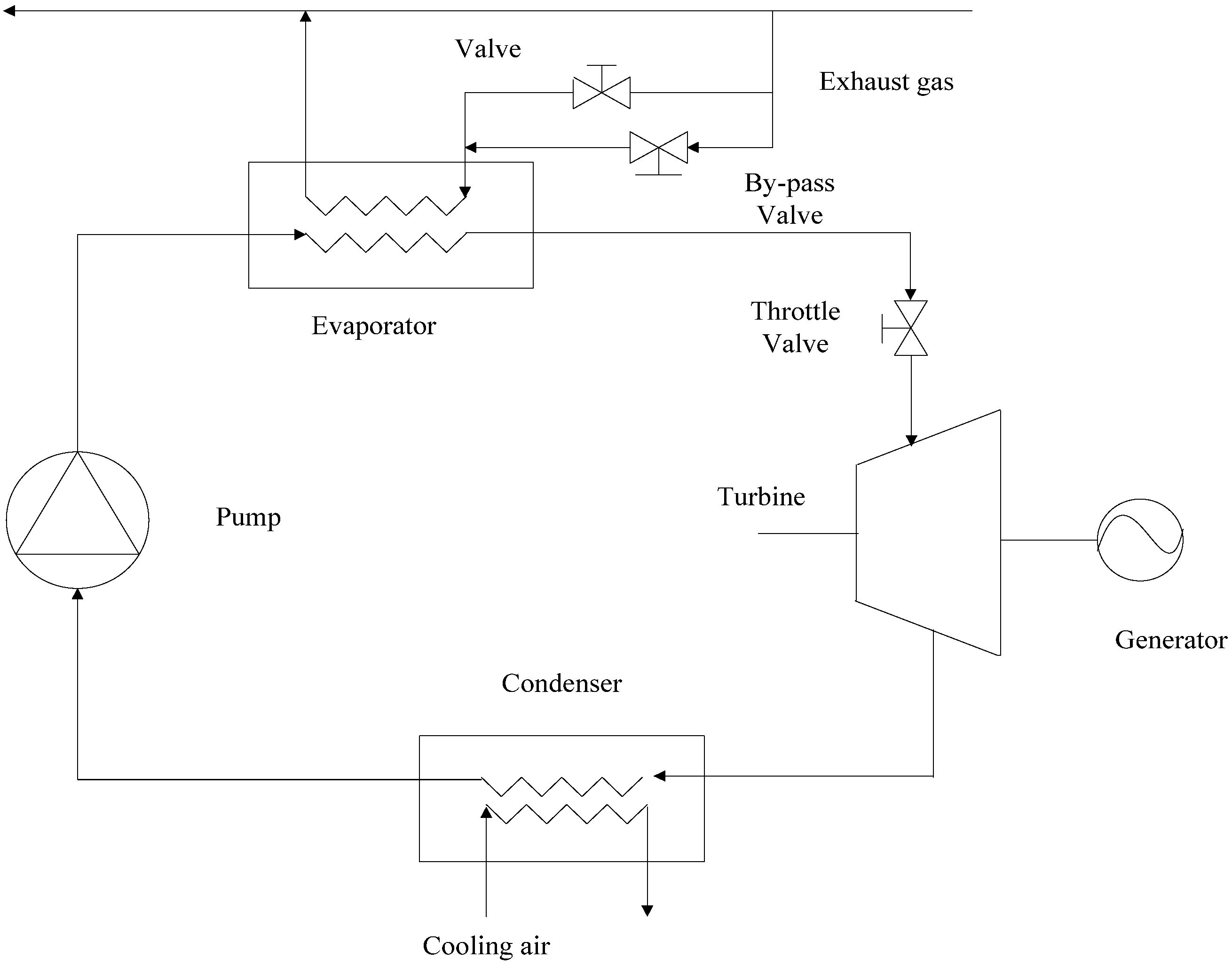
2. System Description

Figure 1 shows the schematic diagram of the ORC based waste heat recovery system, which mainly consists of a turbine expander, an evaporator, an air-cooled condenser and a working fluid pump. The exhaust gas which comes from boiler exchanges heat with the organic working fluid in the evaporator, and the fluid becomes superheated vapor. The working fluid enters into the turbine for expansion and electric power is generated in this unit, subsequently the organic working fluid is condensed into liquid form in an air-cooled condenser. The liquid is re-pressurized by the working fluid pump and then sent into the evaporator to continue the cycle.

Figure 1. A simplified diagram of a waste heat recovery system.

Figure 1. A simplified diagram of a waste heat recovery system.

The ORC-based waste heat recovery system operates following an electric load mode. The level of electric power should be tuned to follow the variations of the electric power demand with sufficient exhaust gas. Meanwhile the system variables must be kept within safe operating limits.

The controlled vector in the proposed control system for the ORC process is selected as y = [N P T], which should be kept within desired operating ranges. Here $\text{N}$ is the output power, $\text{P}$ is the throttle pressure, and $\text{T}$ is the outlet temperature of evaporator. The manipulated vector is u = [μ_T w v_e], where μ_T is the throttle valve position, which can change from 0 to 100%. $\text{w}$ is the motor speed for pump, and v_e is the velocity of the exhaust gas.

3. Model Development via Parameter Identification

To facilitate controller design [26], the ORC system can be adequately represented by a transfer function model. Identification of model parameters is required for the design of active disturbance rejection control. In this work, the parameter identification algorithm used is the same as that in [27] which has the following steps: (1) one or more manipulated variables are modulated to excite the ORC process dynamics, and the input and output data are collected through the experiments; (2) the transfer function model is established by applying a least-squares parameter identification algorithm using the collected data in (1) [28]; (3) verification tests are conducted to validate the model for the ORC system process. If the model prediction is not satisfactory, the model structure will be adjusted for another round of parameter estimation. The whole procedure will repeat until a model with reasonable prediction precision is obtained.

In this work, we used a previously developed ORC model [15] to produce the pseudo-experimental data for parameter estimation study. The state space model of both the evaporator and the condenser was built by moving boundary approach. A static model was built for the expander. The model of the pump model was established according to the performance curve provided by manufacturer. The whole organic Rankine cycle system can then be modeled by integrating the model of each component. Based on these input-output data, the physical model can be reformulated [29] using system identification technique:

$$\{\begin{array}{c}{y}_1^{\left(n_1\right)}={\phi }_1\left({\vartheta }_1,{\vartheta }_2,\cdots ,{\vartheta }_m,u,w_1\right)+b_1{u}_1\\ y_2^{\left(n_2\right)}={\phi }_2\left({\vartheta }_1,{\vartheta }_2,\cdots ,{\vartheta }_m,u,w_{\text{2}}\right)+b_2{u}_2\\ ⋮\\ y_m^{\left(n_m\right)}={\phi }_m\left({\vartheta }_1,{\vartheta }_2,\cdots ,{\vartheta }_m,u,w_m\right)+b_m{u}_m\end{array}$$

(1)

The multivariable system (1) is an m-loop system, where $y_i$ and $u_i$ are the output and input respectively. $w_i$ is the external disturbance. The input gain $b_i$ can be obtained by parameter identification. $y_i^{\left(n_i\right)}$ stands for the $n_i^{th}$ order derivative of $y_i$, $i=1,2,\cdots ,m$. $m$ is the number of controlled variables. Here we consider the general case for multivariable systems, in which the number of manipulated variables is the same as the controlled variables. ${\vartheta }_i$ and $u$ are defined as:

$$\{\begin{array}{c}{\vartheta }_1=\left[y_1^{\left(n_1-1\right)}\left(t\right),y_1^{\left(n_1-2\right)}\left(t\right),\cdots ,y_1\left(t\right)\right]\\ {\vartheta }_2=\left[y_2^{\left(n_2-1\right)}\left(t\right),y_2^{\left(n_2-2\right)}\left(t\right),\cdots ,y_2\left(t\right)\right]\\ ⋮\\ {\vartheta }_m=\left[y_m^{\left(n_m-1\right)}\left(t\right),y_m^{\left(n_m-2\right)}\left(t\right),\cdots ,y_m\left(t\right)\right]\\ u=\left[u_1\left(t\right),u_2\left(t\right),\cdots ,u_m\left(t\right)\right]\end{array}$$

(2)

4. LADRC Algorithm

In the linear active disturbance rejection control (LADRC) framework, uncertainties of the internal dynamics and significant unknown external disturbance is actively estimated using an extended state observer and compensated by the feedback control law in the absence of an accurate plant mode.

We denote:

$$f_i={\phi }_i\left({\vartheta }_1,{\vartheta }_2,\cdots {\vartheta }_m,u,w_i\right)+\left(b_i-b_{0,i}\right)u_i$$

(3)

as the generalized disturbances in the $i^{th}$ loop, where $b_{0,i}$ is the approximate value of $b_i$. Equation (1) can then be rewritten as:

$$\{\begin{array}{c}{y}_1^{\left(n_1\right)}=f_1+b_{0,1}{u}_1\\ y_2^{\left(n_2\right)}=f_2+b_{0,2}{u}_2\\ ⋮\\ y_m^{\left(n_m\right)}=f_m+b_{0,m}{u}_m\end{array}$$

(4)

4.1. Extended State Observer Design

Consider the $i^{th}$ loop in (4):

$$y_i^{\left(n_i\right)}=f_i+b_{0,i}{u}_i$$

(5)

Introduce $f_i$ as an extended state, and denote:

$$\{\begin{array}{c}{x}_{1,i}=y_i\\ x_{2,i}={\dot{y}}_i\\ ⋮\\ x_{n_i,i}=y_i^{\left(n_i-1\right)}\\ x_{n_i+1,i}=f_i\end{array}$$

(6)

Assuming that $f_i$ is differentiable and $h_i={\dot{f}}_i$ is bounded, the state equation of (5) can be rewritten as:

$$\{\begin{array}{l}{\dot{x}}_i=A{x}_i+B{u}_i+D{h}_i\\ y_i=C{x}_i\end{array}$$

(7)

where:

$$x_i={\left[\begin{array}{ccccc}{x}_{1,i}& x_{2,i}& \cdots & x_{n,i}& x_{n+1,i}\end{array}\right]}_{\left(n+1\right)\times 1}^T$$

$$A={\left[\begin{array}{ccccc}0& 1& 0& \cdots & 0\\ 0& 0& 1& \cdots & 0\\ \cdots & \cdots & \cdots & \ddots & ⋮\\ 0& 0& 0& \cdots & 1\\ 0& 0& 0& \cdots & 0\end{array}\right]}_{\left(n+1\right)\times \left(n+1\right)}$$

$$B={\left[\begin{array}{c}0\\ 0\\ ⋮\\ b_{0,i}\\ 0\end{array}\right]}_{\left(n+1\right)\times 1}$$

$$D={\left[\begin{array}{ccccc}0& 0& \cdots & 0& 1\end{array}\right]}_{\left(n+1\right)\times 1}^T$$

$$C={\left[\begin{array}{ccccc}1& 0& \cdots & 0& 0\end{array}\right]}_{\left(n+1\right)\times 1}$$

Based on the state space model (7), $f_i$ can be estimated by the following linear extended state observer (LESO):

$$\{\begin{array}{l}{\dot{\widehat{x}}}_i=A{\widehat{x}}_i+B{u}_i+L_i(x_{1,i}-{\widehat{x}}_{\text{1},i})\\ {\widehat{y}}_i=C{\widehat{x}}_{\text{1},i}\end{array}$$

(8)

where $L_i={\left[\begin{array}{ccccc}{\beta }_{1,i}& {\beta }_{2,i}& \cdots & {\beta }_{n_i,i}& {\beta }_{n_i+1,i}\end{array}\right]}^T$ is the observer gain vector, which determines the accuracy of the estimated state. The characteristic polynomial of the LESO can be represented as a function of ${\omega }_{o,i}$, that is [25]:

$$\begin{array}{l}{\lambda }_{o,i}(s)=\left|sI-\left(A-L_{i}C\right)\right|={\left(s+{\omega }_{0,i}\right)}^{n_i+1}\\ =s^{n_i+1}+{\omega }_{o,i}{\alpha }_{1,i}{s}^{n_i}+\cdots +{\omega }_{o,i}^{n_i}{\alpha }_{n_i,i}s+{\omega }_{o,i}^{n_i+1}{\alpha }_{n_i+1,i}\end{array}$$

(9)

where ${\alpha }_{j,i}=\frac{\left(n_i+1\right)!}{j!\left(n_i+1-j\right)!},j=1,2,\cdots ,n_i+1$. It is clear that ${\omega }_{o,i}$ is the only observer tuning parameter of the $i^{th}$ loop.

4.2. Control Algorithm

Once the observer is designed and well-tuned, the output of the observer, ${\widehat{f}}_i$, should closely track the states of the augmented plant, $f_i$ The control law of the $i^{th}$ loop is given by [24]:

$$u_i=\frac{-{\widehat{f}}_i+u_{0,i}}{b_{0,i}}$$

(10)

Since $f_i\to {\widehat{f}}_i$, then $y_i^{\left(n_i\right)}=\left(f_i-{\widehat{f}}_i\right)+u_{0,i}\approx u_{0,i}$. The feedback control law can be formulated as:

$$u_i=k_{1,i}\left(y_{ri}-{\widehat{x}}_{1,i}\right)+\cdots +k_{n_i,i}\left(y_{ri}^{\left(n_i-1\right)}-{\widehat{x}}_{n_i,i}\right)-y_{ri}^{\left(n_i\right)}$$

(11)

where $y_{ri}$ is the desired trajectory of the $i^{th}$ loop. Then the closed-loop characteristic polynomial is:

$${\lambda }_{c,i}\left(s\right)=s^{n_i}+k_{n_i,i}{s}^{n_i-1}+\cdots +k_{1,i}={\left(s+{\omega }_{c,i}\right)}^{n_i}$$

(12)

where, $k_{j,i}=\frac{n_i!}{\left(j-1\right)!\left(n_i-j+1\right)!}{\omega }_{c,i}^{n_i-j+1},j=1,2,\cdots ,n_i$ is the controller gain, ${\omega }_{c,i}$ is the controller bandwidth of the state feedback system to be optimized.

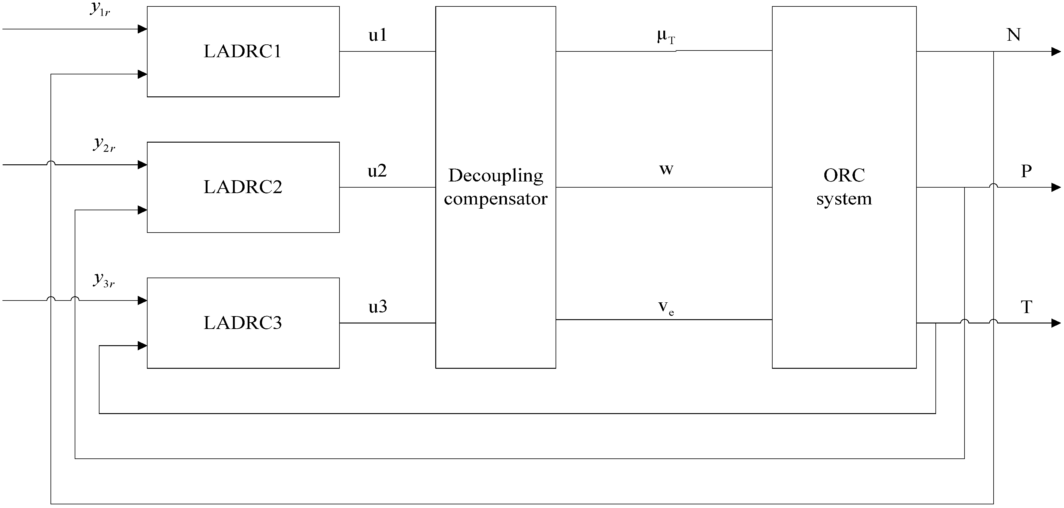
4.3. LADRC of an ORC Process

Figure 2 illustrates the waste heat recovery system with LADRC, in which $u_1,u_2$ and $u_3$ are the corresponding outputs of linear active disturbance rejection controllers. $y_{1r}$, $y_{2r}$ and $y_{3r}$ represent the set-points of power output, evaporating pressure and evaporator outlet temperature, respectively. Since there exists coupling between control loops in the waste heat recovery systems, it is necessary to perform static decoupling before applying LADRC law into the ORC based waste heat recovery system. The controller design procedure can be described as the following steps:

Step 1:

Collect and record the measured data of the ORC output $y_i$ and input $u_i$, $i=1,2,3$.

Step 2:

Obtain the transfer function model by a least-square parameter identification algorithm.

Step 3:

Apply the static decoupling method to the coupled system model.

Step 4:

Design the linear extended state observers for the LADRC controllers.

Step 5:

Tune the control parameter $b_{0,i}$ according to the original plant information.

Step 6:

Select the observer tuning parameter ${\omega }_{o,i}$ as in (9), and controller tuning parameter ${\omega }_{c,i}$ in (12) based on the bandwidth requirement of the closed-loop system.

Figure 2. LADRC for the waste heat recovery system.

Figure 2. LADRC for the waste heat recovery system.

5. Simulation Studies

The following tests were conducted based on a previously developed model [15] to investigate the performance of the proposed LADRC controller for a 100 kW waste heat recovery system with the organic working fluid R245fa. The parameters of the initial operating conditions are the following: $\text{N}=100\hspace{0.17em}\text{kW}$, $\text{P}=2\hspace{0.17em}\text{MPa}$, T = 137.6 °C, ${\text{μ}}_{\text{T}}=0.88$, $\text{w}=2850\text{r}/\text{min}$, ${\text{v}}_{\text{e}}=4.06\text{ m}/\text{s}$. The parameters of the three linear active disturbance rejection controllers are set through experience: $b_{0,1}=45$, ${\omega }_{o,1}=2.68$, ${\omega }_{c,1}=0.67$; $b_{0,2}=160$, ${\omega }_{o,2}=2.68$, ${\omega }_{c,2}=0.67$; $b_{0,3}=190$, ${\omega }_{o,3}=4$ and ${\omega }_{c,3}=1$.

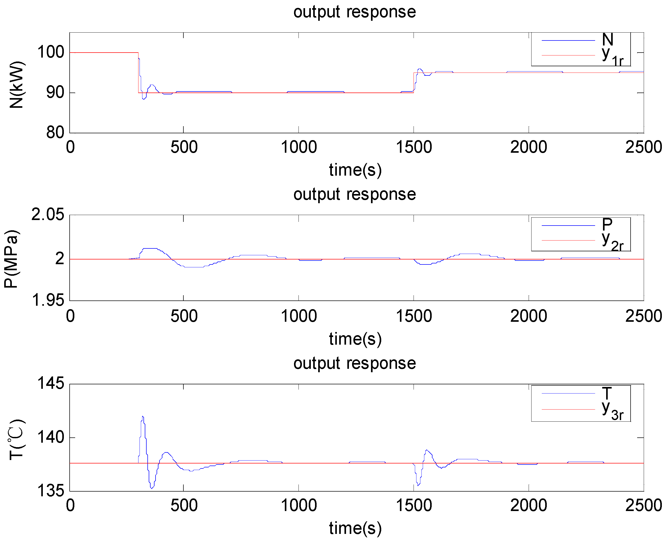
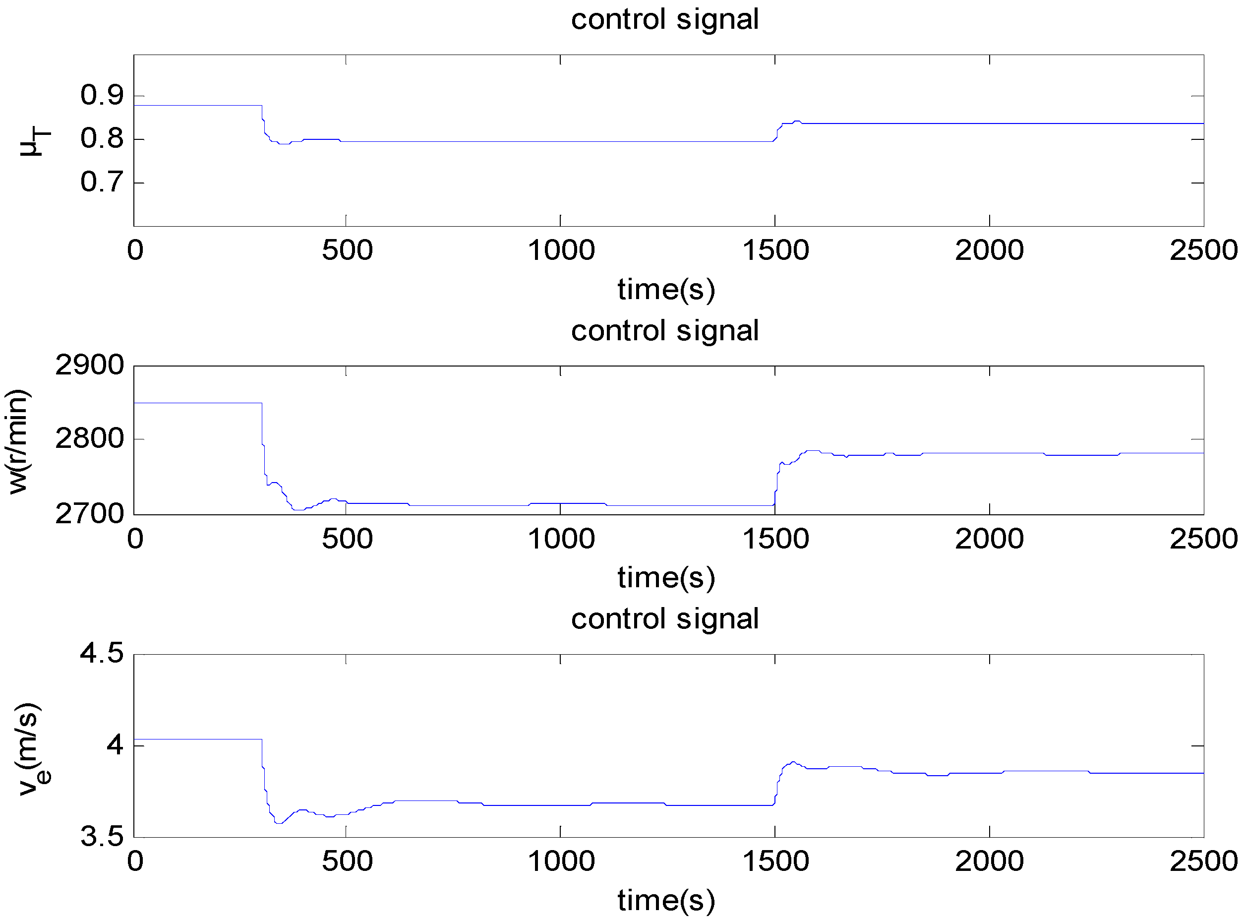
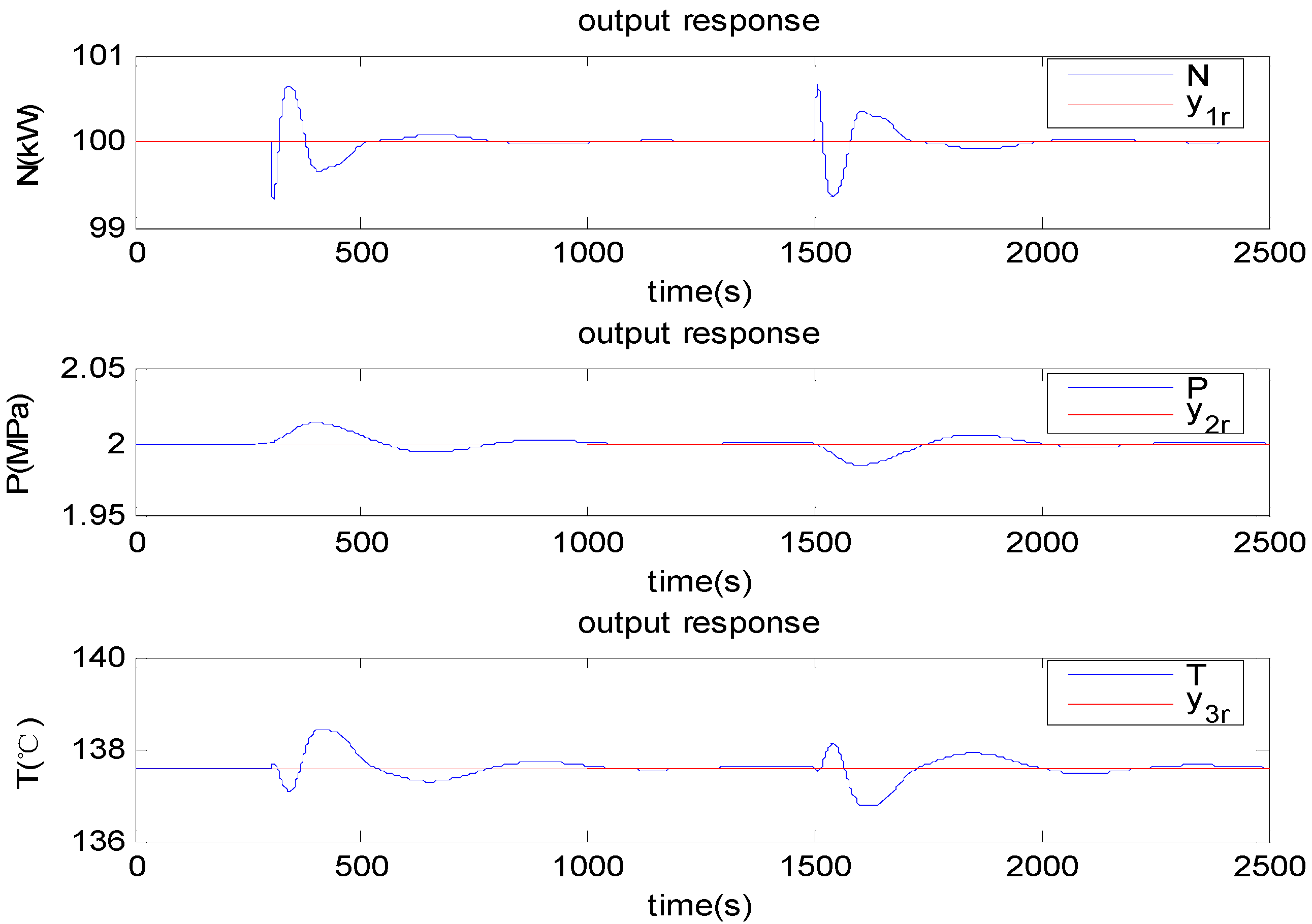
5.1. Tracking Ability Test

5.1.1. Tracking the Set-point of Power Output

In order to test the tracking performance for the power output under the nominal working conditions, the set-point of power output (load demand) was first decreased from 100 kW to 90 kW at t = 300 s, then increased to 95 kW at t = 1500 s. The responses of output variables and the variations of control variables are shown in Figure 3 and Figure 4 respectively.

Through the experimental results, the proposed LDARC has shown to be able to provide satisfactory load demand swiftly and accurately track the desired output for the waste heat recovery system in response to the load demand variations. The maximum deviation of the power output is less than 2 kW in Figure 3. It also shows the response of the throttle pressure and the superheated temperature at outlet of the evaporator when the load demand varies, their maximum deviations from the set-points are less than 0.015 MPa and 6 °C respectively, and the proposed controllers drive them back to their set-points within a short period of time. It can also be seen from the simulation results that the variation of the controlled signals is very small during the testing process.

Figure 3. Responses of controlled variables.

Figure 3. Responses of controlled variables.

Figure 4. Responses of manipulated variables.

Figure 4. Responses of manipulated variables.

5.1.2. Tracking the Set-point of Evaporator Pressure

In order to make the test of tracking evaporator pressure at the nominal working condition, the set-point of evaporator pressure was first decreased by 1000 Pa at t = 300 s, then increased by 500 Pa at t = 1500 s. The responses of output variables and the variations of control variables are shown in Figure 5 and Figure 6 respectively.

As shown in Figure 5, the proposed control strategy provides a good tracking performance. The maximum deviation of evaporator pressure is less than 0.001 MPa. It can be seen that the load demand and the superheated temperature deviate from their set-points when the evaporator pressure varies, their maximum deviations are not more than 0.02 kW, 0.1 °C respectively, and the proposed controller drives them back to the set-points quickly.

Figure 5. Responses of controlled variables.

Figure 5. Responses of controlled variables.

Figure 6. Responses of manipulated variables.

Figure 6. Responses of manipulated variables.

5.1.3. Tracking the Set-point of Evaporator Temperature

In this test, the set-point of the evaporator temperature was decreased by 2 °C at t = 300 s, and then increased by 1 °C at t = 1500 s. The responses of output variables and control variables are illustrated in Figure 7 and Figure 8 respectively.

Figure 7 shows that the evaporator temperature can be controlled to follow the set-points in a timely manner. The maximum deviation of the evaporator temperature is less than 0.5 °C during the test. The load demand and the evaporator pressure deviate from their set-points when the evaporator temperature varies, but their maximum deviations are less than 1 kW and 0.001 MPa respectively. This clearly demonstrates the good control performance of the proposed LDARC strategy.

Figure 7. Responses of controlled variables.

Figure 7. Responses of controlled variables.

Figure 8. Responses of manipulated variables.

Figure 8. Responses of manipulated variables.

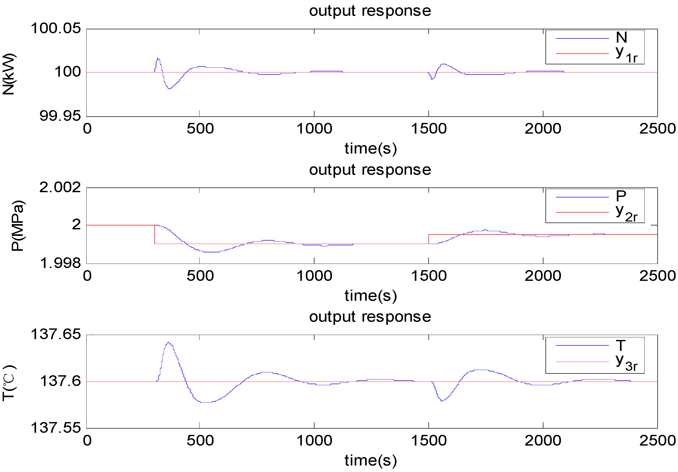
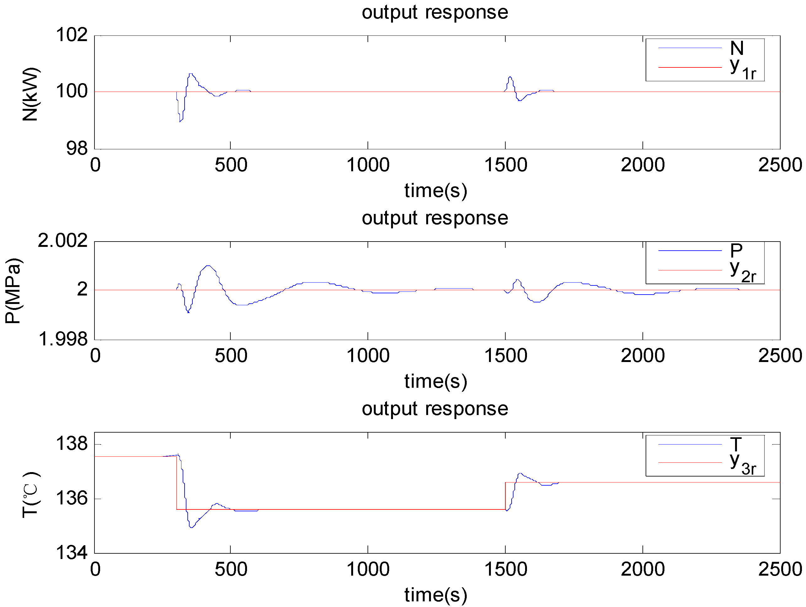
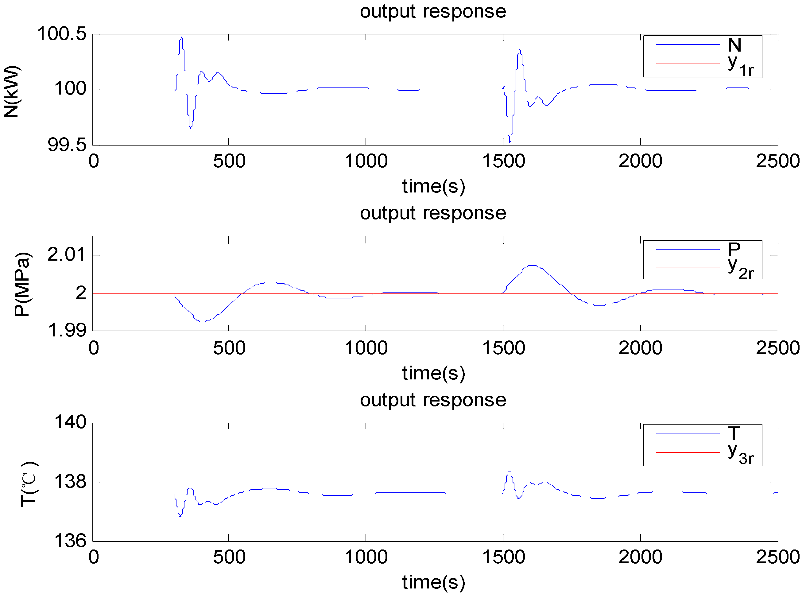
5.2. Disturbance Rejection Test

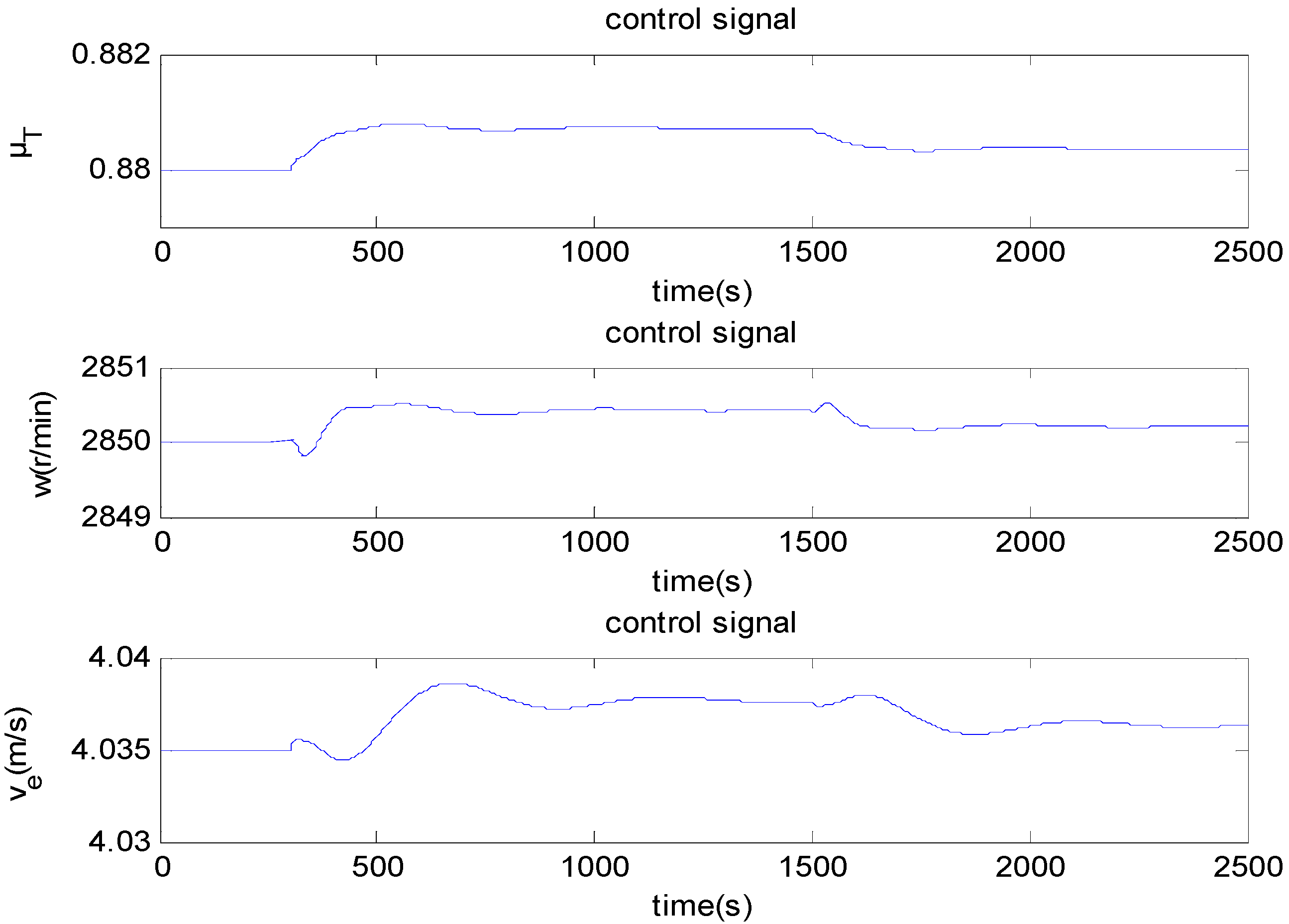
5.2.1. Disturbance in the Throttle Valve Position

Consider the situation that a step disturbance is imposed on the throttle valve position when the waste heat recovery system operates in a steady state. In this simulation, a step decrease of 1% was introduced to the throttle valve position at t = 300 s and a step increase of 1% made at t = 1,500 s. The responses of the three controlled variables are shown in Figure 9.

Figure 9. Responses of controlled variables.

Figure 9. Responses of controlled variables.

The variation (disturbance) of the throttle valve position at t = 300 s and 1500 s causes the deviations of the power output, the throttle pressure and the superheated temperature at outlet of the evaporator from their original tracks. The maximum deviations of the three variables are 0.8 kW, 0.02 MPa and 3 °C, respectively. The control action drives these three signals back to their set values after a short period of time, which suggests that the waste heat recovery system is well controlled in the presence of disturbance to the throttle valve position.

5.2.2. Disturbance to the Velocity of Exhaust Gas

In this simulation, a disturbance of the flow rate of exhaust gas is imposed by changing the position of the by-pass valve at the inlet of evaporator when the waste heat recovery system operates in a steady state. A step decrease of 1% at t = 300 s and a step increase of 1% at t = 1500 s were introduced to the velocity of the exhaust gas. The responses of the controlled variables are shown in Figure 10. The disturbance to the velocity of exhaust gas leads to the deviations of the power output, the throttle pressure and the superheated temperature at the outlet of the evaporator, however, under the proposed control scheme, the maximum deviations of these three outputs are only 0.5 kW, 0.01 MPa and 1 °C, respectively. In spite of the disturbance to the exhaust gas, the control action manages to drive the three variables back to their original values within a reasonably short period of time.

Figure 10. Responses of controlled variables.

Figure 10. Responses of controlled variables.

6. Conclusions

In this paper, the novel LADRC scheme is successfully applied to the design of decentralized controllers for the waste heat recovery system. The ORC process model is achieved by parameter identification technique. Simulation results demonstrate that the proposed control algorithm can provide good tracking performance and well handle disturbances for the waste heat recovery systems.

It should be noted that the design of the control strategy without requiring an accurate mathematical model for the waste heat recovery system is a significant progress for this type of processes. A static coupling method was designed based on the simplified linear ORC model which captured the essential dynamics and interaction of the system. This practical control strategy is easy to understand and implement, making it an appealing method to real applications.

References

1. Hung, T.C.; Shai, T.Y.; Wang, S.K. A review of Organic Rankine Cycles (ORCs) for the recovery of low-grade waste heat. Appl. Energy 1997, 6, 661–667. [Google Scholar] [CrossRef]
2. Tchanche, B.F.; Lambrinos, G.; Frangoudakis, A.; Papadakis, G. Low-grade heat conversion into power using Organic Rankine Cycles—a review of various applications. Renew. Sustain. Energy Rev. 2011, 15, 3963–3979. [Google Scholar] [CrossRef]
3. Wang, E.H.; Zhang, H.G.; Fan, B.Y.; Ouyang, M.G. Study of working fluid selection of organic Rankine cycle (ORC) for engine waste heat recovery. Energy 2011, 36, 3406–3418. [Google Scholar] [CrossRef]
4. Hung, T.C.; Wang, S.K.; Kuo, C.H.; Pei, B.S.; Tsai, K.F. A study of organic working fluids on system efficiency of an ORC using low-grade energy sources. Energy 2010, 35, 1403–1411. [Google Scholar] [CrossRef]
5. Luján, J.M.; Serrano, J.R.; Dolz, V.; Sánchez, J. Model of the expansion process for R245fa in an Organic Rankine Cycle (ORC). Appl. Therm. Eng. 2012, 40, 248–257. [Google Scholar] [CrossRef]
6. Wei, D.H.; Lu, X.S.; Lu, Z.; Gu, J.M. Dynamic modeling and simulation of an Organic Rankine Cycle (ORC) system for waste heat recovery. Appl. Therm. Eng 2008, 28, 1216–1224. [Google Scholar] [CrossRef]
7. Quoilin, S.; Aumann, R.; Grill, A.; Schuster, A.; Lemort, V.; Spliethoff, H. Dynamic modeling and optimal control strategy of waste heat recovery Organic Rankine Cycles. Appl. Energy 2011, 88, 2183–2190. [Google Scholar] [CrossRef]
8. Vaja, I.; Gambarotta, A. Dynamic model of an organic Rankine cycle system. Part I—Mathematical description of main components. In Proceedings of 23rd International Conference on Efficiency, Cost, Optimization, Simulation and Environment Impact of Energy, Lausanne, Switzerland, 14–17 June 2010.
9. Vaja, I.; Gambarotta, A. Dynamic Model of an Organic Rankine Cycle System. Part II—The full Model: Description and Validation. In Proceedings of 23rd International Conference on Efficiency, Cost, Optimization, Simulation and Environment Impact of Energy, Lausanne, Switzerland, 14–17 June 2010.
10. Wei, D.H.; Lu, X.S.; Lu, Z.; Gu, J.M. Performance analysis and optimization of Organic Rankine Cycle (ORC) for waste heat recovery. Energy Convers. Manag. 2007, 48, 1113–1119. [Google Scholar] [CrossRef]
11. Clemente, S.; Micheli, D.; Reini, M.; Taccan, R. Energy efficiency analysis of Organic Rankine Cycles with scroll expanders for cogenerative applications. Appl. Energy 2012, 97, 792–801. [Google Scholar] [CrossRef]
12. Quoilin, S.; Lemort, V.; Lebrun, J. Experimental study and modeling of an Organic Rankine Cycle using scroll expender. Appl. Energy 2010, 87, 1260–1268. [Google Scholar] [CrossRef]
13. Lemort, V.; Quoilin, S.; Cuevas, C.; Lebrun, J. Testing and modeling a scroll expander integrated into an Organic Rankine Cycle. Appl. Therm. Eng. 2009, 29, 3094–3102. [Google Scholar] [CrossRef]
14. Desai, N.B.; Bandyopadhyay, S. Process integration of organic Rankine cycle. Energy 2009, 34, 1674–1686. [Google Scholar] [CrossRef]
15. Zhang, J.H.; Zhang, W.F.; Hou, G.L.; Fang, F. Dynamic modeling and multivariable control of Organic Rankine Cycle in waste heat utilizing processes. Comput. Math. Appl. 2012, 64, 908–921. [Google Scholar] [CrossRef]
16. Zhang, J.H.; Li, Y.; Wang, Z.F.; Hou, G.L. Dynamic characteristics and predictive control for evaporator. In Proceedings of the 2011 International Conference on Advanced Mechatronic Systems, Zhengzhou, China, 11–13 August 2011; pp. 513–518.
17. Hou, G.L.; Sun, R.; Hu, G.Q.; Zhang, J.H. Supervisory predictive control of evaporator in Organic Rankine Cycle (ORC) system for waste heat recovery. In Proceedings of the 2011 International Conference on Advanced Mechatronic Systems, Zhengzhou, China, 11–13 August 2011; pp. 306–311.
18. Han, J. Nonlinear state error feedback control. Control Des. 1995, 10, 221–225. [Google Scholar]
19. Zhou, W.K.; Gao, Z.Q. An active disturbance rejection approach to tension and velocity regulations in web processing lines. In Proceedings of 16th IEEE International Conference on Control Applications, Singapore, 1–3 October 2007; pp. 842–848.
20. Zheng, Q.; Dong, L.; Gao, Z. Control and Time-Varying Rotation Rate Estimation of Vibrational MEMS Gyroscopes. In Proceedings of IEEE Multi-conference on Systems and Control, Singapore, 1–3 October 2007; pp. 118–123.
21. Huang, H.P.; Wu, L.Q.; Han, J.Q.; Gao, F.; Lin, Y.J. A new synthesis method for unit coordinated control system in thermal power plant-ADRC control scheme. In Proceedings of 2004 International Conference on Power System Technology, Singapore, 21–24 November 2004; pp. 133–138.
22. Dong, L.L.; Zhang, Y.; Gao, Z.Q. A robust decentralized load frequency controller for interconnected power systems. ISA Trans. 2012, 51, 410–419. [Google Scholar] [CrossRef]
23. Gao, Z.Q. Scaling and parameterization based controller tuning. In Proceedings of American Control Conference, Denver, CO, USA, 4–6 June 2003; pp. 4996–4996.
24. Goforth, F.; Zheng, Q.; Gao, Z.Q. A novel practical control approach for rate independent hysteretic systems. ISA Trans. 2012, 51, 477–484. [Google Scholar] [CrossRef] [PubMed]
25. Zheng, Q.; Chen, Z.Z.; Gao, Z.Q. A practical approach to disturbance decoupling control. Control. Eng. Pract. 2009, 17, 1016–1025. [Google Scholar] [CrossRef]
26. Ananth, I.; Chidambaram, M. Closed-loop identification of transfer function model for unstable systems. J. Franklin Inst. 1999, 1055–1061. [Google Scholar] [CrossRef]
27. Haley, T.A.; Mulvaney, S.J. On-line system identification and control design of an extrusion cooking process: Part 1. System identification. Food Control. 2000, 11, 103–120. [Google Scholar] [CrossRef]
28. Xiao, Y.S.; Ding, F.; Zhou, Y.; Li, M.; Dai, J.Y. On consistency of recursive least squares identification algorithms for controlled auto-regression models. Appl. Math. Model. 2008, 32, 2207–2215. [Google Scholar] [CrossRef]
29. Zheng, Q.; Chen, Z.Z.; Gao, Z.Q. A dynamic decoupling control approach and its applications to chemical processes. In Proceedings of American Control Conference, New York, NY, USA, 9–13 July 2007; pp. 5176–5181.