An Efficient Drift-Flux Closure Relationship to Estimate Liquid Holdups of Gas-Liquid Two-Phase Flow in Pipes

Abstract

The reliable predictions of liquid holdup and pressure drop are essential for pipeline design in oil and gas industry. In this study, the drift-flux approach is utilized to calculate liquid holdups. This approach has been widely used in formulation of the basic equations for multiphase flow in pipelines. Most of the drift-flux models have been developed on an empirical basis from the experimental data. Even though, previous studies showed that these models can be applied to different flow pattern and pipe inclination, when the distribution parameter is flow pattern dependent. They are limited to a set of fluid properties, pipe geometries and operational conditions. The objective of this study is to develop a new drift-flux closure relationship for prediction of liquid holdups in pipes that can be easily applied to a wide range of flow conditions. The developed correlation is compared with nine available correlations from literatures, and validated using the TUFFP (Fluid Flow Projects of University of Tulsa) experimental datasets and OLGA (OiL and GAs simulator supplied by SPTgroup) steady-state synthetic data generated by OLGA Multiphase Toolkit. The developed correlation performs better in predicting liquid holdups than the available correlations for a wide range of flow conditions.

1. Introduction

The predictions of liquid holdup and pressure drop are essential for pipeline design in the oil and gas industry. A drift-flux approach has been widely used in formulation of the basic equations for multiphase flow in pipelines. This approach, for simplicity, considers the flowing phases as a mixture. This, thereby, ignores the detailed characteristics of two-phase flow. The drift-flux model needs additional constitutive equations for the viscous shear stress, and closure relationships for the Reynolds stress and for the slip velocity between the phases to improve its accuracy and applicability [1,2].

Most of the previous correlations have been developed on an empirical basis from the experimental data. Nicklin [3] showed a strong relationship between the in-situ gas velocity and the mixture velocity based on his experimental study in two-phase bubble flow in vertical pipes. Zuber and Findlay [4] corroborated Nicklin [3] for vertical flow in an annular flow and a slug flow. They predicted the average volumetric concentration with a general expression as a function of the distribution parameter and the weighted average drift velocity. Coddington and Macian [5] evaluated the applicability of the widely used correlations based on Zuber and Findlay’s [4] drift-flux model. They used various experimental data taken from rod bundle, level swell and boil-off experiments performed at 9 different experimental facilities. Their results confirmed the validity and the usefulness of drift-flux model. França and Lahey [6], using air-water experimental data, verified the use of drift-flux model for all flow patterns observed in horizontal gas-liquid flow. For these conditions, the distribution parameter and the drift velocity were flow pattern dependent. Recently, Danielson and Fan [7] demonstrated the validity of this relationship for stratified, annular, slug and dispersed bubble flows in a large diameter and high pressure horizontal flow.

Fabre and Line [8] introduced a correlation for the distribution parameter in slug flow using a liquid Reynolds number. The proposed correlation showed fair agreement with the measured flow distribution parameter in the transition zone between laminar and turbulent flow. Goda et al. [9] investigated the distribution parameter and the drift velocity for downward two-phase flows. They derived the distribution parameter by taking into account the effect of the downward mixture volumetric flux on the phase distribution. Ishii [10] used vertical upward churn-turbulent flow equation for the drift velocity over all of flow regimes. The proposed model was validated with 463 data points showing a good agreement.

In recent experiments, Shi et al. [11] determined drift-flux parameters (i.e., the distribution parameter and the drift velocity) for oil-water-gas flow using large diameter (150 mm diameter) pipe apparatus. They proposed a unified two and three-phase flow model. The new model improved the prediction accuracy for oil and water holdups. Shen et al. [12] used a 200 mm diameter vertical pipe and characterized two-phase flow patterns into bubbly, churn and slug. They found that the existing correlations of bubble flow pattern predicted the distribution parameter properly but failed on predicting the velocity properly.

In summary, all the available drift-flux models are limited to a specified set of fluid properties, pipe geometries and operational conditions. The objective of this study is to develop a new closure relationship for the drift-flux parameters that can be easily applied to a wide range of conditions. The developed correlation is compared with nine available correlations from literatures, and validated using the TUFFP (Fluid Flow Projects of University of Tulsa) experimental datasets and OLGA (OiL and GAs simulator supplied by SPTgroup) steady-state synthetic data generated by the OLGA Multiphase Toolkit.

2. Methodology

2.1. Procedure to Predict Liquid Holdups Using Drift-Flux Closure Relationship Correlation

A general equation of the drift-flux closure relationship is given as follows:

$$u_G=C_0{u}_M+u_D$$

(1)

In Equation (1), $u_G$ is the gas velocity expressed as $u_G=u_{SG}/{\alpha }_G$, $u_M$ is mixture velocity given by $u_M=u_{SG}+u_{SL}$ where $u_{SG}$ and $u_{SL}$ are superficial gas and liquid velocities, respectively. $C_0$ and $u_D$ represent the drift-flux parameters, namely, the distribution parameter and the drift velocity, respectively. By definition, Equation (1) can be rearranged as follows:

$$H_L=1-\frac{u_{SG}}{C_0(u_{SL}+u_{SG})+u_D}$$

(2)

The liquid holdup, $H_L$, can be estimated by drift-flux model if the parameters $C_0$ and $u_D$ are known.

This study proposes the new equation set of these two parameters for drift-flux model, and compares the proposed model with previously developed comparative models.

2.1.1. Datasets and Comparative Models

Experimental and synthetic datasets were prepared to examine the performances of the considered models. More than 1000 data from seven TUFFP two-phase experiments were considered. OLGA Multiphase Toolkit was used to generate 463 steady-state synthetic data. As a tool included in OLGA software, which is provided by SPTgroup, Multiphase Toolkit is able to analyze a fully developed steady state flow using the OLGAS point model. In this study, 463 input conditions for the synthetic data set are randomly generated in the ranges of Table 1; pipe diameter is kept constant (0.0762 m or 3.0 in.). With these input conditions, liquid holdups and pressure gradients are calculated from OLGA Multiphase Toolkit. Table 2 summarizes the experimental datasets, which cover wide ranges of inclination angle, pipe diameter, fluid property and flow pattern. As it can be seen in Table 1 and Table 2, the database covers a wide range of fluid properties, pipe geometries and flow conditions.

Table 1. Random variables used in generating the synthetic data.

Variable	Inclination angle (Degree)	Gas superficial velocity (m/s)	Liquid superficial velocity (m/s)	Gas density (kg/m3)	Liquid density (kg/m3)	Gas viscosity (N-s/m2)	Liquid viscosity (N-s/m2)	Liquid/Gas surface tension (N/m)
Max. value	10	15.0	1.000	3.000	820.00	0.000018	0.002	0.032
Min. value	-10	0.1	0.001	2.000	800.00	0.000018	0.001	0.032

Table 1. Random variables used in generating the synthetic data.

Variable	Inclination angle (Degree)	Gas superficial velocity (m/s)	Liquid superficial velocity (m/s)	Gas density (kg/m3)	Liquid density (kg/m3)	Gas viscosity (N-s/m2)	Liquid viscosity (N-s/m2)	Liquid/Gas surface tension (N/m)
Max. value	10	15.0	1.000	3.000	820.00	0.000018	0.002	0.032
Min. value	-10	0.1	0.001	2.000	800.00	0.000018	0.001	0.032

Table 2. Description of the sources and the properties for the experimental data.

Property	Experimental data
	Vigneron et al. [13]	Fan [14]	Magrini [15]	Gokcal [16,17]	Felizola [18]	Roumazeilles [19]
Fluid type	Gas-liquid	Gas-liquid	Gas-liquid	Gas-liquid	Gas-liquid	Gas-liquid
# of data	30	351	140	356	89	113
Length (m)	420	112.8	17.5	18.9	15	19
Pipe diameter (m)	0.0779	0.0508(Small) 0.1496(Large)	0.0762	0.0508	0.051	0.051
Inclination angle (°)	0	−2,−1,0,	0,10,20,45,	0	0,10,20,30,40,	0,−3,−5,
(−:downward, +:upward)		+1,+2	60,75,90		50,60,70,80,90	−10,−20,−30
Gas flow rate (Sm3/h)	14.16∼451.65	35.96∼187.53 (Small) 311.90∼1626.32 (Large)	600.87∼1351.15	0.66∼148.12	2.87∼24.71	6.72∼68.81
Liquid flow rate (m3/h)	0.33∼14.13	0.0019∼0.38 (Small) 0.016∼3.30 (Large)	0.056∼0.66	0.073∼12.84	0.37∼10.96	6.50∼17.93
Gas density (kg/m3)	1.942∼4.230	1.166∼2.902	1.31∼1.71	1.12∼4.50	2.09∼3.48	1.938∼3.306
Liquid density (kg/m3)	809.7	947∼1000	995∼997	768.7∼885	796.8∼810	800.923∼823.349
Gas viscosity (Pa·s)	0.0000187	0.000018	0.000018	0.000018	0.0000187	0.000019
Liquid viscosity (Pa·s)	0.05527	0.001	0.001	0.178∼0.601	0.00128∼0.00167	0.0014∼0.00219

Table 2. Description of the sources and the properties for the experimental data.

Property	Experimental data
	Vigneron et al. [13]	Fan [14]	Magrini [15]	Gokcal [16,17]	Felizola [18]	Roumazeilles [19]
Fluid type	Gas-liquid	Gas-liquid	Gas-liquid	Gas-liquid	Gas-liquid	Gas-liquid
# of data	30	351	140	356	89	113
Length (m)	420	112.8	17.5	18.9	15	19
Pipe diameter (m)	0.0779	0.0508(Small) 0.1496(Large)	0.0762	0.0508	0.051	0.051
Inclination angle (°)	0	−2,−1,0,	0,10,20,45,	0	0,10,20,30,40,	0,−3,−5,
(−:downward, +:upward)		+1,+2	60,75,90		50,60,70,80,90	−10,−20,−30
Gas flow rate (Sm3/h)	14.16∼451.65	35.96∼187.53 (Small) 311.90∼1626.32 (Large)	600.87∼1351.15	0.66∼148.12	2.87∼24.71	6.72∼68.81
Liquid flow rate (m3/h)	0.33∼14.13	0.0019∼0.38 (Small) 0.016∼3.30 (Large)	0.056∼0.66	0.073∼12.84	0.37∼10.96	6.50∼17.93
Gas density (kg/m3)	1.942∼4.230	1.166∼2.902	1.31∼1.71	1.12∼4.50	2.09∼3.48	1.938∼3.306
Liquid density (kg/m3)	809.7	947∼1000	995∼997	768.7∼885	796.8∼810	800.923∼823.349
Gas viscosity (Pa·s)	0.0000187	0.000018	0.000018	0.000018	0.0000187	0.000019
Liquid viscosity (Pa·s)	0.05527	0.001	0.001	0.178∼0.601	0.00128∼0.00167	0.0014∼0.00219

This work presents a comparative analysis of the nine models; the first one is a simple linear model where and $C_0$ and $u_D$ are constant. The others are from the literatures, including Zuber and Findlay [4], Ishii [10], Liao et al. [20], Jowitt et al. [21], Sonnenburg [22], Bestion [23], Kataoka and Ishii [24], and Shi et al. [11] models. Table 3 contains the expressions of the comparative models used in this study.

Table 3. Expressions of the comparative models.

Authors	Model expressions
Zuber and Findlay [4]	$C_0=1.2$
	$u_D=1.53{\left(\frac{g\sigma \Delta \rho }{{{\rho }_L}^2}\right)}^{1/4}$
Ishii [10]	For churn turbulent flow:
	$C_0=1.2-0.2\sqrt{\frac{{\rho }_G}{{\rho }_L}}(1-\exp (-18{\alpha }_G))$
	$u_D=\left(C_0-1\right)u_M+\sqrt{2}{\left(\frac{g\sigma \Delta \rho }{{{\rho }_L}^2}\right)}^{1/4}$
Liao et al. [20]	For churn turbulent flow:
	$C_0=1.2-0.2\sqrt{\frac{{\rho }_G}{{\rho }_L}}\left(1-\exp (-18{\alpha }_G)\right)$
	$u_D=0.33{\left(\frac{g\sigma \Delta \rho }{{{\rho }_L}^2}\right)}^{1/4}$
Jowitt et al. [21]	$C_0=1+0.796\exp \left(-0.061\sqrt{\frac{{\rho }_G}{{\rho }_L}}\right)$
	$u_D=0.034\left(\sqrt{\frac{{\rho }_G}{{\rho }_L}}-1\right)$
Sonnenburg [22]	$C_0=1+\left(0.32-0.32\sqrt{\frac{{\rho }_G}{{\rho }_L}}\right)$
	$u_D=\frac{C_0\left(1-C_0{\alpha }_G\right)}{\left(C_0{\alpha }_G/\sqrt{gd\Delta \rho /{\rho }_G}\right)+\left(1-C_0{\alpha }_G/\sqrt{gd\Delta \rho /{\rho }_L}\right)}$
Bestion [23]	$C_0=1$
	$u_D=0.188\sqrt{\frac{gd\Delta \rho }{{\rho }_G}}$
Kataoka and Ishii [24]	$C_0=1.2-0.2\sqrt{\frac{{\rho }_G}{{\rho }_L}}$
	$D_H=\frac{d}{\sqrt{\sigma /g\Delta \rho }}$, $N_{\mu L}=\frac{{\mu }_L}{{\left({\rho }_L\sigma \sqrt{\sigma /(g\Delta \rho )}\right)}^{0.5}}$
	Low viscosity case: $N_{\mu L}⩽2.25\times {10}^{-3}$
	$u_D=0.0019D_H^{0.809}{\left(\frac{{\rho }_G}{\rho L}\right)}^{-0.157}{N}_{\mu L}^{-0.562}$ for $D_H⩽30$
	$u_D=0.030{\left(\frac{{\rho }_G}{\rho L}\right)}^{-0.157}{N}_{\mu L}^{-0.562}$ for $D_H⩾30$
	Higher viscosity case: $N_{\mu L}>2.25\times {10}^{-3}$
	$u_D=0.92{\left(\frac{{\rho }_G}{\rho L}\right)}^{-0.157}$ for $D_H⩾30$
Shi et al. [11]	$C_0=\frac{C}{1+(C-1){\gamma }^2}$
	$0\le \gamma \le 1$, $1\le C\le 1.2$
	$u_D=\frac{(1-{\alpha }_G{C}_0)C_{0}K\left({\alpha }_G\right)V_c}{{\alpha }_G{C}_0\sqrt{\frac{{\rho }_G}{{\rho }_L}}+1-{\alpha }_G{C}_0}$
	$K\left({\alpha }_G\right)=1.53/C_0$ for ${\alpha }_G\le 0.2$
	$K\left({\alpha }_G\right)=$ critical Kutateladze number for ${\alpha }_G\ge 0.4$
	$V_c={\left(\frac{g\sigma \Delta \rho }{{{\rho }_L}^2}\right)}^{1/4}$
Fabre and Line [8]	$C_0=\frac{2.27}{1+{(\mathrm{Re}/1000)}^2}+\frac{1.2}{1+{(1000/\mathrm{Re})}^2}$

Table 3. Expressions of the comparative models.

Authors	Model expressions
Zuber and Findlay [4]	$C_0=1.2$
	$u_D=1.53{\left(\frac{g\sigma \Delta \rho }{{{\rho }_L}^2}\right)}^{1/4}$
Ishii [10]	For churn turbulent flow:
	$C_0=1.2-0.2\sqrt{\frac{{\rho }_G}{{\rho }_L}}(1-\exp (-18{\alpha }_G))$
	$u_D=\left(C_0-1\right)u_M+\sqrt{2}{\left(\frac{g\sigma \Delta \rho }{{{\rho }_L}^2}\right)}^{1/4}$
Liao et al. [20]	For churn turbulent flow:
	$C_0=1.2-0.2\sqrt{\frac{{\rho }_G}{{\rho }_L}}\left(1-\exp (-18{\alpha }_G)\right)$
	$u_D=0.33{\left(\frac{g\sigma \Delta \rho }{{{\rho }_L}^2}\right)}^{1/4}$
Jowitt et al. [21]	$C_0=1+0.796\exp \left(-0.061\sqrt{\frac{{\rho }_G}{{\rho }_L}}\right)$
	$u_D=0.034\left(\sqrt{\frac{{\rho }_G}{{\rho }_L}}-1\right)$
Sonnenburg [22]	$C_0=1+\left(0.32-0.32\sqrt{\frac{{\rho }_G}{{\rho }_L}}\right)$
	$u_D=\frac{C_0\left(1-C_0{\alpha }_G\right)}{\left(C_0{\alpha }_G/\sqrt{gd\Delta \rho /{\rho }_G}\right)+\left(1-C_0{\alpha }_G/\sqrt{gd\Delta \rho /{\rho }_L}\right)}$
Bestion [23]	$C_0=1$
	$u_D=0.188\sqrt{\frac{gd\Delta \rho }{{\rho }_G}}$
Kataoka and Ishii [24]	$C_0=1.2-0.2\sqrt{\frac{{\rho }_G}{{\rho }_L}}$
	$D_H=\frac{d}{\sqrt{\sigma /g\Delta \rho }}$, $N_{\mu L}=\frac{{\mu }_L}{{\left({\rho }_L\sigma \sqrt{\sigma /(g\Delta \rho )}\right)}^{0.5}}$
	Low viscosity case: $N_{\mu L}⩽2.25\times {10}^{-3}$
	$u_D=0.0019D_H^{0.809}{\left(\frac{{\rho }_G}{\rho L}\right)}^{-0.157}{N}_{\mu L}^{-0.562}$ for $D_H⩽30$
	$u_D=0.030{\left(\frac{{\rho }_G}{\rho L}\right)}^{-0.157}{N}_{\mu L}^{-0.562}$ for $D_H⩾30$
	Higher viscosity case: $N_{\mu L}>2.25\times {10}^{-3}$
	$u_D=0.92{\left(\frac{{\rho }_G}{\rho L}\right)}^{-0.157}$ for $D_H⩾30$
Shi et al. [11]	$C_0=\frac{C}{1+(C-1){\gamma }^2}$
	$0\le \gamma \le 1$, $1\le C\le 1.2$
	$u_D=\frac{(1-{\alpha }_G{C}_0)C_{0}K\left({\alpha }_G\right)V_c}{{\alpha }_G{C}_0\sqrt{\frac{{\rho }_G}{{\rho }_L}}+1-{\alpha }_G{C}_0}$
	$K\left({\alpha }_G\right)=1.53/C_0$ for ${\alpha }_G\le 0.2$
	$K\left({\alpha }_G\right)=$ critical Kutateladze number for ${\alpha }_G\ge 0.4$
	$V_c={\left(\frac{g\sigma \Delta \rho }{{{\rho }_L}^2}\right)}^{1/4}$
Fabre and Line [8]	$C_0=\frac{2.27}{1+{(\mathrm{Re}/1000)}^2}+\frac{1.2}{1+{(1000/\mathrm{Re})}^2}$

3. Results and Discussion

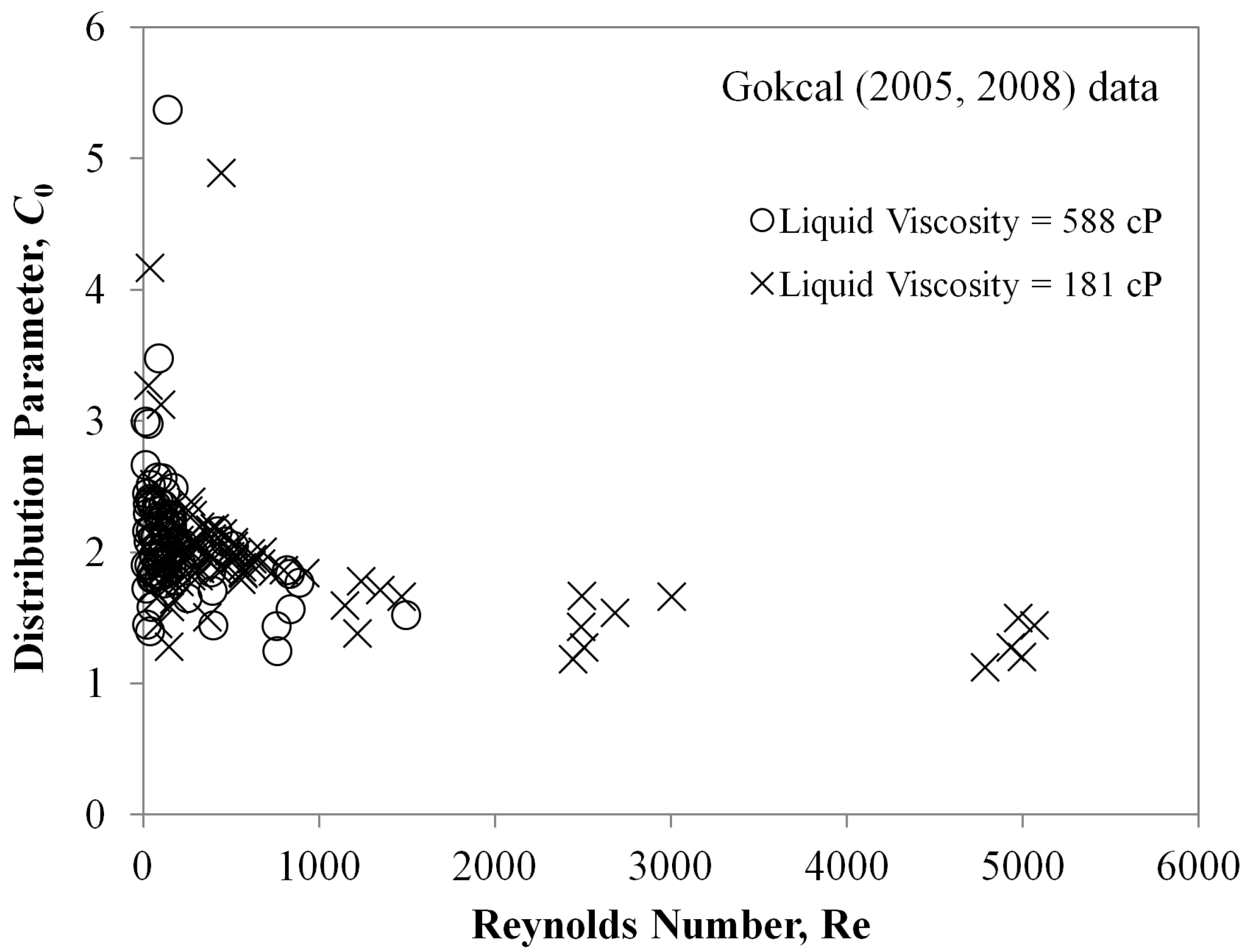
3.1. New Closure Relationship

In previous studies for low viscosity liquids, the distribution parameter ($C_0$) tends to have a value range of $1.0<C_0<1.2$. As can be seen in Figure 1, Gokcal [17] suggested a larger distribution parameter ($C_0$ ∼ 2) for low liquid Reynolds number ($\mathrm{Re}=\left({\rho }_L{u}_{M}d\right)/{\mu }_L$, ${\rho }_L$ is the liquid density, ${\mu }_L$ is the liquid viscosity, and d is the pipe inner-diameter). For large Reynolds numbers ($\mathrm{Re}>1,000$), the distribution parameter tends to vary between a 1.0 and 1.2. Unfortunately, no medium viscosity data has been found to corroborate the transition region between these two regimes. Based on this variation of the distribution parameter with Reynolds number, the new closure relationship correlation in this work is combining Fabre and Line [8], which is function of Reynolds number, and Ishii [10], which is relatively simple and accurate, as follows:

$$C_0=\frac{2}{1+{(\mathrm{Re}/1000)}^2}+\frac{1.2-0.2\sqrt{{\rho }_G/{\rho }_L}(1-\exp (-18{\alpha }_G)}{1+{(1000/\mathrm{Re})}^2}$$

(3)

where ${\alpha }_G$ is the gas void fraction. For laminar flow region, the value of 2 is implemented instead of 2.27 in the original Fabre and Line [8] model according to Figure 1. For turbulent flow region, 1.2 in Fabre and Line [8] model is replaced to Ishii [10] model for better performance. The inclusion of the liquid Reynolds number allows the prediction of the distribution parameter for a larger range of liquid viscosities.

Figure 1. Distribution parameter ($C_0$) for Gokcal [16,17] data.

Figure 1. Distribution parameter ($C_0$) for Gokcal [16,17] data.

The drift velocity ($u_D$) can be estimated by a modified version of Zuber and Findlay [4] model to consider the inclination angle effects as given below.

$$u_D=A\cos \theta +B{\left(\frac{g\sigma \Delta \rho }{{{\rho }_L}^2}\right)}^{1/4}\sin \theta$$

(4)

where σ was the surface tension between gas and liquid phase; and θ is the pipe inclination angle. The coefficients A and B of Equation (4) were obtained from a regression analysis between the predicted liquid holdup and the measured liquid holdup. For the experimental database presented in this study, the resultant values of A and B are given as 0.0246 and 1.606, respectively. On the other hand, the synthetic data yield $A=-0.191$ and $B=12.59$.

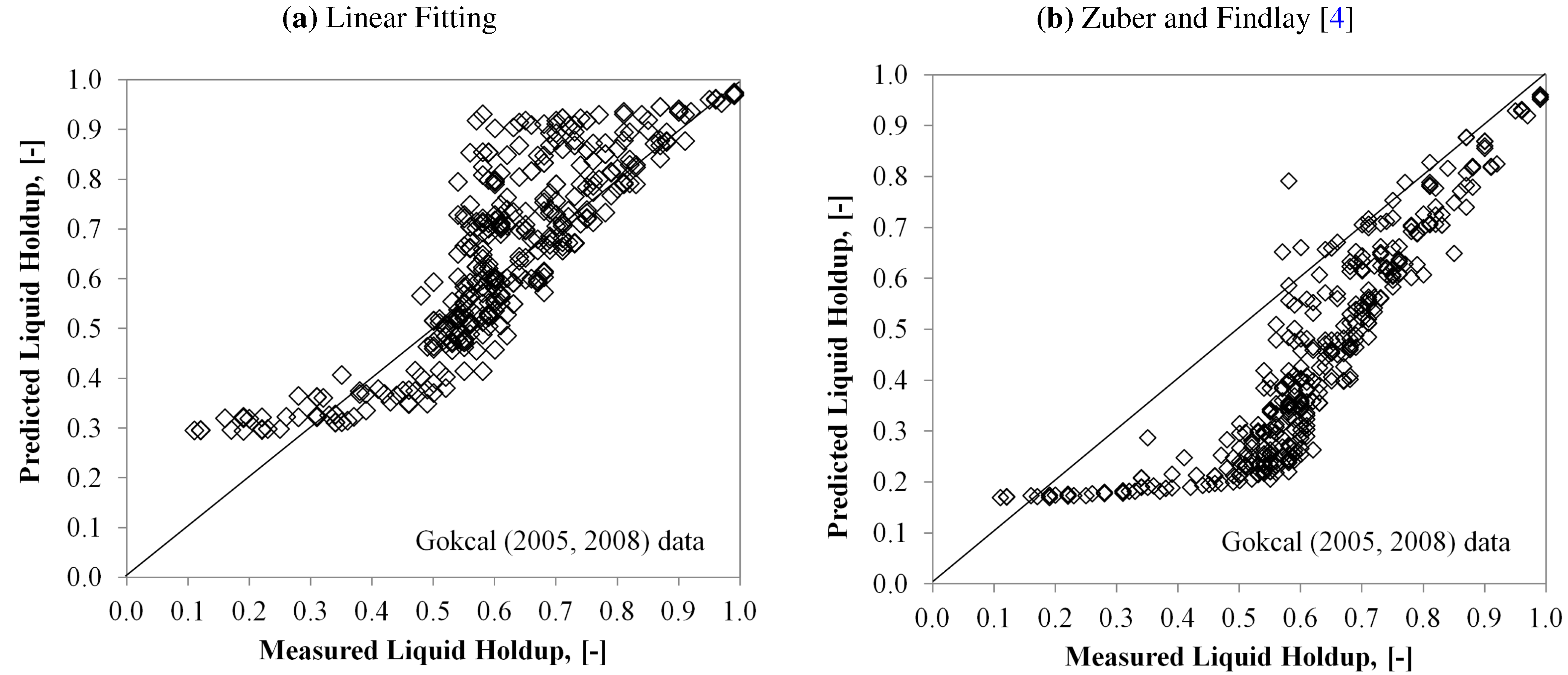
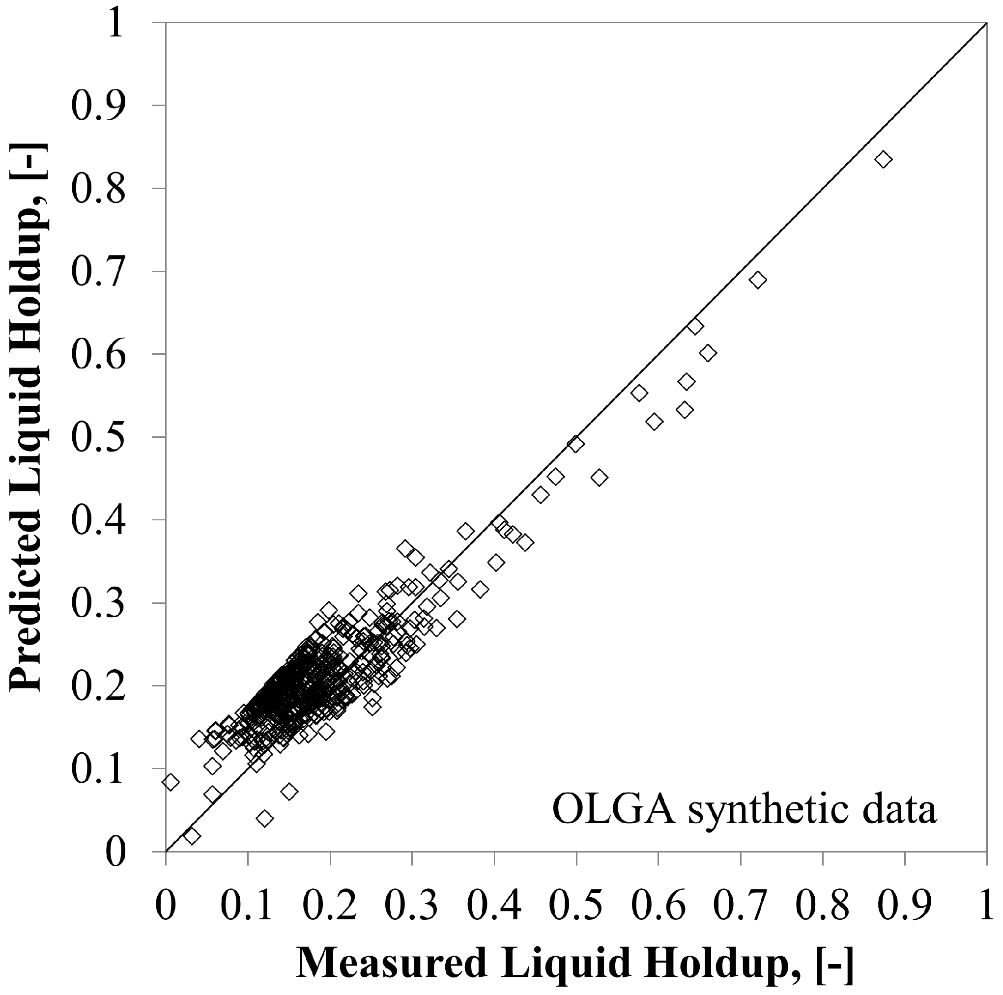
3.2. Prediction Accuracy of the Developed Model

The accuracy of the models is measured by mean absolute errors and standard deviations. Mean absolute errors are calculated by arithmetic means of absolute difference between measured and predicted liquid holdups. Table 4 summarizes the performances of 9 models from literature and the proposed model for liquid holdups predictions, and presents the mean absolute error of the models and the standard deviations. The proposed model has predicted the liquid holdup better than the other models. Its mean absolute error is 0.09584, which is similar to the linear fitting, and the standard deviation is 0.05684. Linear model gives smaller errors with slightly larger standard deviations. Linear model uses constant parameters obtained by typical regression analysis of measured data and calculated value, and thereby highly depends on the given data. It has a limitation for general application. In Section 3.3, this will be explained.

Figure 2 shows the prediction performance of the linear model and the Zuber and Findlay [4] model against Gokcal [16,17] experimental data for a relatively high viscosity liquid. In the case of Gokcal [16,17] dataset, the linear model relatively performed better for $0.3<H_L<0.7$ than the Zuber and Findlay [4] model. However, for $0.7<H_L$, the Zuber and Findlay [4] model performed relatively better than the linear fitting model. Figure 2 shows a limitation of model application for a wide range of flow conditions.

Figure 2. Two prediction performance examples of the comparative models against the experimental datasets: (a) Linear model; and (b) Zuber and Findlay [4] model. Each model shows relatively better performance for different range of liquid holdups; linear fitting for $H_L<0.7$ and the Zuber and Findlay [4] model for $H_L>0.7$. This shows their limitation in applying to a wide range of flow conditions.

Figure 2. Two prediction performance examples of the comparative models against the experimental datasets: (a) Linear model; and (b) Zuber and Findlay [4] model. Each model shows relatively better performance for different range of liquid holdups; linear fitting for $H_L<0.7$ and the Zuber and Findlay [4] model for $H_L>0.7$. This shows their limitation in applying to a wide range of flow conditions.

The proposed model performs consistently well for the entire range of liquid holdup. Figure 3 shows the correlation predictions against Gokcal [16,17] experimental data. Figure 4 presents correlation predictions against OLGA synthetic data having 0.0398 of mean absolute error, which is smaller than that against Gokcal [16,17] experimental data.

Figure 3. Prediction performance of the proposed model against the Gokcal [16,17] experimental dataset. The proposed model shows the best prediction performance compared with the comparative models; mean absolute error is 0.04234 and its standard deviation is 0.03755.

Figure 3. Prediction performance of the proposed model against the Gokcal [16,17] experimental dataset. The proposed model shows the best prediction performance compared with the comparative models; mean absolute error is 0.04234 and its standard deviation is 0.03755.

Figure 4. Prediction performance of the proposed model against the OLGA synthetic dataset. The proposed model shows good prediction performance; mean absolute error is 0.0398, which is smaller than that against experimental data in Figure 3.

Figure 4. Prediction performance of the proposed model against the OLGA synthetic dataset. The proposed model shows good prediction performance; mean absolute error is 0.0398, which is smaller than that against experimental data in Figure 3.

Table 4. Performance comparison for liquid holdup predictions. The proposed model shows the second smallest mean absolute error (0.09584) and the smallest standard deviation (0.05684) among the models.

Model	Closure relationship	Mean absolute error (Standard deviation)							All data
		Vigneron et al. [13]	Fan(Small) [14]	Fan(Large) [14]	Magrini [15]	Felizola [18]	Roumazeilles [19]	Gokcal [16,17]
The proposed model	Equations (3) & (4)	0.10684	0.14673	0.12803	0.15619	0.06612	0.08246	0.04234	0.09584
		(0.06402)	(0.01221)	(0.02506)	(0.00369)	(0.05319)	(0.04446)	(0.03755)	(0.05684)
The comparative models	Linear fitting	0.12319	0.06109	0.03886	0.00330	0.18692	0.06161	0.12400	0.08272
		(0.07298)	(0.04256)	(0.02519)	(0.00315)	(0.08584)	(0.02402)	(0.08556)	(0.07984)
	Zuber and Findlay[4] ($C_0=1.2$)	0.09071	0.16578	0.14449	0.16257	0.05842	0.09978	0.17548	0.14708
		(0.06240)	(0.01303)	(0.02425)	(0.00353)	(0.04735)	(0.04860)	(0.09578)	(0.07076)
	Ishii [10]	0.08492	0.16846	0.14830	0.15934	0.08251	0.10632	0.13716	0.13759
		(0.05610)	(0.01564)	(0.02397)	(0.00334)	(0.05699)	(0.04519)	(0.08224)	(0.05987)
	Liao et al. [20]	0.11962	0.09651	0.00288	0.15477	0.29511	0.18035	0.20556	0.14988
		(0.10789)	(0.07193)	(0.00522)	(0.00385)	(0.08743)	(0.05203)	(0.09229)	(0.10885)
	Jowitt et al. [21]	0.08620	0.20468	0.13984	0.14487	0.14258	0.15421	0.09646	0.13645
		(0.06638)	(0.01893)	(0.02522)	(0.00624)	(0.06498)	(0.05117)	(0.06434)	(0.06028)
	Sonnenburg [22]	0.15635	0.26991	0.27515	0.24188	0.20085	0.19128	0.08344	0.18856
		(0.23257)	(0.02589)	(0.02690)	(0.00332)	(0.23483)	(0.10169)	(0.06600)	(0.12271)
	Bestion [23]	0.15688	0.16070	0.27793	0.06203	0.30781	0.14751	0.15181	0.17560
		(0.14045)	(0.07811)	(0.06747)	(0.01472)	(0.08495)	(0.01611)	(0.09781)	(0.10610)
	Kataoka and Ishii [24]	0.08992	0.16002	0.14859	0.15897	0.06834	0.10145	0.15957	0.14214
		(0.06066)	(0.01327)	(0.02397)	(0.00338)	(0.05245)	(0.04586)	(0.09203)	(0.06595)
	Shi et al. [11]	0.19551	0.01404	0.02644	0.00701	0.07616	0.02951	0.24502	0.10324
		(0.08131)	(0.01138)	(0.02163)	(0.00381)	(0.05076)	(0.02098)	(0.13133)	(0.13101)

Table 4. Performance comparison for liquid holdup predictions. The proposed model shows the second smallest mean absolute error (0.09584) and the smallest standard deviation (0.05684) among the models.

Model	Closure relationship	Mean absolute error (Standard deviation)							All data
		Vigneron et al. [13]	Fan(Small) [14]	Fan(Large) [14]	Magrini [15]	Felizola [18]	Roumazeilles [19]	Gokcal [16,17]
The proposed model	Equations (3) & (4)	0.10684	0.14673	0.12803	0.15619	0.06612	0.08246	0.04234	0.09584
		(0.06402)	(0.01221)	(0.02506)	(0.00369)	(0.05319)	(0.04446)	(0.03755)	(0.05684)
The comparative models	Linear fitting	0.12319	0.06109	0.03886	0.00330	0.18692	0.06161	0.12400	0.08272
		(0.07298)	(0.04256)	(0.02519)	(0.00315)	(0.08584)	(0.02402)	(0.08556)	(0.07984)
	Zuber and Findlay[4] ($C_0=1.2$)	0.09071	0.16578	0.14449	0.16257	0.05842	0.09978	0.17548	0.14708
		(0.06240)	(0.01303)	(0.02425)	(0.00353)	(0.04735)	(0.04860)	(0.09578)	(0.07076)
	Ishii [10]	0.08492	0.16846	0.14830	0.15934	0.08251	0.10632	0.13716	0.13759
		(0.05610)	(0.01564)	(0.02397)	(0.00334)	(0.05699)	(0.04519)	(0.08224)	(0.05987)
	Liao et al. [20]	0.11962	0.09651	0.00288	0.15477	0.29511	0.18035	0.20556	0.14988
		(0.10789)	(0.07193)	(0.00522)	(0.00385)	(0.08743)	(0.05203)	(0.09229)	(0.10885)
	Jowitt et al. [21]	0.08620	0.20468	0.13984	0.14487	0.14258	0.15421	0.09646	0.13645
		(0.06638)	(0.01893)	(0.02522)	(0.00624)	(0.06498)	(0.05117)	(0.06434)	(0.06028)
	Sonnenburg [22]	0.15635	0.26991	0.27515	0.24188	0.20085	0.19128	0.08344	0.18856
		(0.23257)	(0.02589)	(0.02690)	(0.00332)	(0.23483)	(0.10169)	(0.06600)	(0.12271)
	Bestion [23]	0.15688	0.16070	0.27793	0.06203	0.30781	0.14751	0.15181	0.17560
		(0.14045)	(0.07811)	(0.06747)	(0.01472)	(0.08495)	(0.01611)	(0.09781)	(0.10610)
	Kataoka and Ishii [24]	0.08992	0.16002	0.14859	0.15897	0.06834	0.10145	0.15957	0.14214
		(0.06066)	(0.01327)	(0.02397)	(0.00338)	(0.05245)	(0.04586)	(0.09203)	(0.06595)
	Shi et al. [11]	0.19551	0.01404	0.02644	0.00701	0.07616	0.02951	0.24502	0.10324
		(0.08131)	(0.01138)	(0.02163)	(0.00381)	(0.05076)	(0.02098)	(0.13133)	(0.13101)

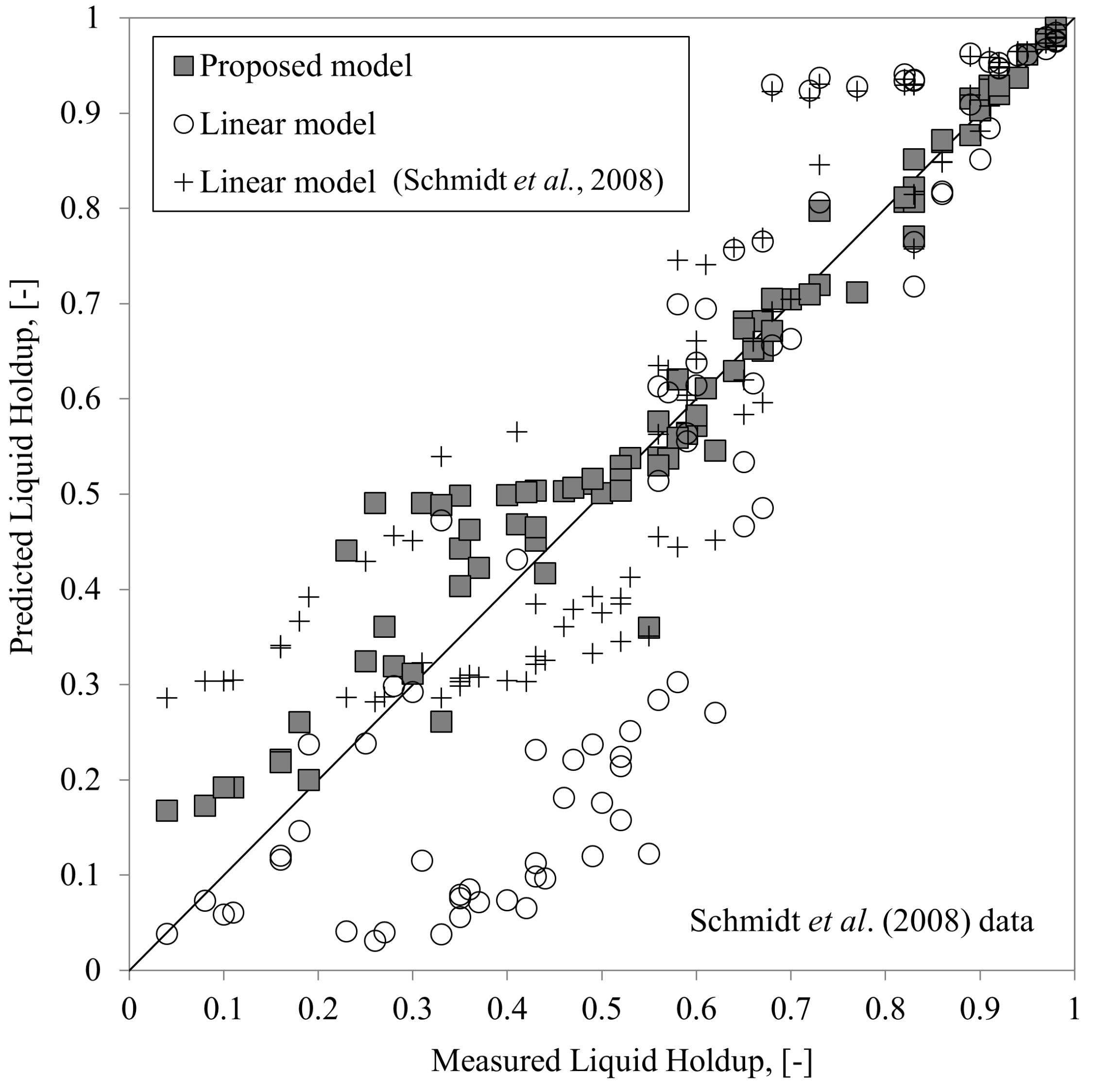
3.3. Validation of the New Proposed Model

Schmidt et al. [25] performed high-viscosity two-phase flow experiments in a vertical upward pipe. Their experimental data are not used in the development of the proposed model parameters, which are A and B in Equation (4). Their data are used to test the applicability of the new model. It has distinctive flow conditions, i.e., high viscosity liquid, for a whole range of liquid holdups ($0<H_L<1$).

Figure 5 shows the liquid holdup predictions of both the proposed model and the linear model, which showed the smallest mean absolute error for the test of comparative models. In Figure 5 and Table 5, “Linear fitting” denotes that the drift-flux parameters, the distribution parameter ($C_0$) and drift velocity ($u_D$), are taken from a linear fitting of the other experimental data, while “Linear Fitting (Schmidt et al., 2008)” uses the drift-flux parameters taken from a linear fitting of Schmidt et al. [25] data. It is reasonable that the latter gives better result than the former because of its high dependence on the data used in the regression analysis.

The proposed model clearly performs better. Table 5 summarizes the results for the liquid holdup estimations of various models and correlations against Schmidt et al. [25] data. The proposed model shows the best prediction accuracy in terms of mean absolute error and its standard deviation.

Figure 5. Prediction performance of the proposed model comparing linear models against the Schmidt et al. [25] experimental dataset. Linear model shows the smallest mean absolute error in model performance comparison against all available experimental datasets; mean absolute error of the proposed model is 0.09584, and that of linear model is 0.08272. However, The proposed model shows better prediction performance than linear models against the Schmidt et al. [25] experimental data, which is performed with high viscosity liquid; mean absolute error of the proposed model is 0.04960, that of linear model is 0.12270, and that of linear model (Schmidt et al., 2008) is 0.6950.

Figure 5. Prediction performance of the proposed model comparing linear models against the Schmidt et al. [25] experimental dataset. Linear model shows the smallest mean absolute error in model performance comparison against all available experimental datasets; mean absolute error of the proposed model is 0.09584, and that of linear model is 0.08272. However, The proposed model shows better prediction performance than linear models against the Schmidt et al. [25] experimental data, which is performed with high viscosity liquid; mean absolute error of the proposed model is 0.04960, that of linear model is 0.12270, and that of linear model (Schmidt et al., 2008) is 0.6950.

Table 5. Performance comparison of the proposed model and comparative models against the Schmidt et al.[25] experimental data set.

Model	Closure relationship	Mean abs. err.	Std. dev.
The proposed model	Equations (3) & (4)	0.04340	0.04960
The comparative models	Linear fitting	0.13955	0.12270
	Linear fitting (Schmidt et al., 2008)	0.09124	0.06950
	Zuber and Findlay[4] ($C_0=1.2$)	0.15163	0.10307
	Ishii[10]	0.12767	0.09334
	Liao et al.[20]	0.14036	0.09303
	Jowitt et al.[21]	0.11045	0.08086
	Sonnenburg[22]	0.09612	0.07091
	Bestion[23]	0.13291	0.09604
	Kataoka and Ishii[24]	0.14364	0.09971
	Shi et al.[11]	0.21452	0.15823

Table 5. Performance comparison of the proposed model and comparative models against the Schmidt et al.[25] experimental data set.

Model	Closure relationship	Mean abs. err.	Std. dev.
The proposed model	Equations (3) & (4)	0.04340	0.04960
The comparative models	Linear fitting	0.13955	0.12270
	Linear fitting (Schmidt et al., 2008)	0.09124	0.06950
	Zuber and Findlay[4] ($C_0=1.2$)	0.15163	0.10307
	Ishii[10]	0.12767	0.09334
	Liao et al.[20]	0.14036	0.09303
	Jowitt et al.[21]	0.11045	0.08086
	Sonnenburg[22]	0.09612	0.07091
	Bestion[23]	0.13291	0.09604
	Kataoka and Ishii[24]	0.14364	0.09971
	Shi et al.[11]	0.21452	0.15823

4. Conclusions

The new liquid holdup closure relationship using drift-flux approach has been developed and validated with experimental data. The proposed closure relationship was compared with nine comparative models using datasets covering a wide range of operating conditions, flow patterns, pipeline inclination angles, and fluid properties. Over this wide range, the proposed closure relationship performed consistently well and better than the other models or correlations in liquid holdup predictions.

References

1. Prado, M.G. A Block Implicit Numerical Solution Technique for Two-Phase Multidimensional Steady State Flow. Ph.D. Dissertation, The University of Tulsa, Tulsa, OK, USA, 1995. [Google Scholar]
2. Ishii, M.; Hibiki, T. Thermo-Fluid Dynamics of Two-Phase Flow; Springer: New York, NY, USA, 2005. [Google Scholar]
3. Nicklin, D.J. Two-phase bubble flow. Chem. Eng. Sci. 1962, 17, 693–702. [Google Scholar] [CrossRef]
4. Zuber, N.; Findlay, J.A. Average volumetric concentration in two-phase flow Systems. J. Heat Transf. 1965, 87, 453–468. [Google Scholar] [CrossRef]
5. Coddington, P.; Macian, R. A study of the performance of void fraction correlations used in the context of drift-flux two-phase flow models. Nucl. Eng. Des. 2002, 215, 199–216. [Google Scholar] [CrossRef]
6. França, F.; Lahey, R.T. The use of drift-flux techniques for the analysis of horizontal two-phase flows. Int. J. Multiph. Flow 1992, 18, 787–801. [Google Scholar] [CrossRef]
7. Danielson, T.J.; Fan, Y. Relationship between mixture and two-fluid models. In Preceedings of 14th International Conference on Multiphase Production Technology, Cannes, France, 17–19 June 2009; Volume 14, pp. 479–490.
8. Fabre, J.; Line, A. Modeling of two-phase slug flow. Annu. Rev. Fluid Mech. 1992, 24, 21–46. [Google Scholar] [CrossRef]
9. Goda, H.; Hibiki, T.; Kim, S.; Ishii, M.; Uhle, J. Drift-flux model for downward two-phase flow. Int. J. Heat Mass Transf. 2003, 46, 4835–4844. [Google Scholar] [CrossRef]
10. Ishii, M. One Dimensional Drift-Flux Model and Constitutive Equations for Relative Motion between Phases in Various Two-Phase Flow Regimes; Technical Report for Argonne National Laboratory: Lemont, IL, USA, 1977. [Google Scholar]
11. Shi, H.; Holmes, J.; Diaz, L.; Durlofsky, L.J.; Aziz, K. Drift-flux parameters for three-phase steady-state flow in wellbores. In Proceedings of SPE Annual Technical Conference and Exhibition, Houston, TX, USA, 26–29 September 2004; Society of Petroleum Engineers: Allen, TX, USA, 2005; pp. 130–137. [Google Scholar]
12. Shen, X.; Matsui, R.; Mishima, K.; Nakamura, H. Distribution parameter and drift velocity for two-phase flow in a large diameter pipe. Nucl. Eng. Des. 2010, 240, 3991–4000. [Google Scholar] [CrossRef]
13. Vigneron, F.; Sarica, C.; Brill, J.P. Experimental analysis of imposed two-phase flow transients in horizontal pipelines. In Preceedings of the BHR Group 7th International Conference, Cannes, France, 7–9 June 1995; pp. 199–217.
14. Fan, Y. An Investigation of Low Liquid Loading Gas-Liquid Stratified Flow in Near-Horizontal Pipes. Ph.D. Disseration, University of Tulsa, Tulsa, OK, USA, 2005. [Google Scholar]
15. Magrini, K.L. Liquid Entrainment in Aannular Gas-Liquid Flow in Inclined Pipes. Master’s Thesis, University of Tulsa, Tulsa, OK, USA, 2009. [Google Scholar]
16. Gokcal, B. Effects of High Viscosity on Two-Phase Oil-Gas Flow Behaviour in Horizontal Pipes. Master’s Thesis, University of Tulsa, Tulsa, OK, USA, 2005. [Google Scholar]
17. Gokcal, B. An Experimental and Theoretical Investigation of Slug Flow for High Oil Viscosity in Horizontal Pipes. Ph.D. Dissertation, University of Tulsa, Tulsa, OK, USA, 2008. [Google Scholar]
18. Felizola, H. Slug Flow in Extended Reach Directional Wells. Master’s Thesis, University of Tulsa, Tulsa, OK, USA, 1992. [Google Scholar]
19. Roumazeilles, P. An Experimental Study of Downward Slug Flow in Inclined Pipes. Master’s Thesis, University of Tulsa, Tulsa, OK, USA, 1994. [Google Scholar]
20. Liao, L.; Parlos, A.; Griffith, P. Heat Transfer, Carryover and Fall Back in PWR Steam Generators during Transients; Technical Report NUREG/CR-4376 EPRI-NP-4298; Department of Nuclear Engineering, Massachusetts Institute of Technology: Cambridge, MA, USA, 1985. [Google Scholar]
21. Pearson, K.; Cooper, C.; Jowitt, D. The THETIS 80% Blocked Cluster Experiment, Part 5: Level Swell Experiments; Technical Report for AEEW-R; AEEE Winfrith Safety and Engineering Science Division: London, UK, 1984. [Google Scholar]
22. Sonnenburg, H.G. Full-range drift-flux model base on the combination of drift-flux theory with envelope theory. In Preceedings of 4th International Topical Meeting on Nuclear Reactor Thermal-Hydraulics (NURETH-4), Karlsruhe, Germany, 10–13 October 1989; Volume 2, pp. 1003–1009.
23. Bestion, D. The physical closure laws in the CATHARE code. Nucl. Eng. Des. 1990, 124, 229–245. [Google Scholar] [CrossRef]
24. Kataoka, I.; Ishii, M. Drift flux model for large diameter pipe and new correlation for pool void fraction. Int. J. Heat Mass Transf. 1987, 30, 1927–1939. [Google Scholar]
25. Schmidt, J.; Giesbrecht, H.; van der Geld, C.W.M. Phase and velocity distributions in vertically upward high-viscosity two-phase flow. Int. J. Multiph. Flow 2008, 34, 363–374. [Google Scholar] [CrossRef]