Numerical Simulation of Methane Production from Hydrates Induced by Different Depressurizing Approaches

Abstract

Several studies have demonstrated that methane production from hydrate-bearing porous media by means of depressurization-induced dissociation can be a promising technique. In this study, a 2D axisymmetric model for simulating the gas production from hydrates by depressurization is developed to investigate the gas production behavior with different depressurizing approaches. The simulation results showed that the depressurization process with depressurizing range has significant influence on the final gas production. On the contrary, the depressurizing rate only affects the production lifetime. More amount of cumulative gas can be produced with a larger depressurization range or lowering the depressurizing rate for a certain depressurizing range. Through the comparison of the combined depressurization modes, the Class 2 (all the hydrate dissociation simulations are performed by reducing the initial system pressure with the same depressurizing range initially, then to continue the depressurization process conducted by different depressurizing rates and complete when the system pressure decreases to the atmospheric pressure) is much superior to the Class 1 (different depressurizing ranges are adopted in the initial period of the gas production process, when the pressure is reduced to the corresponding value of depressurization process at the different depressurizing range, the simulations are conducted at a certain depressurizing rate until the pressure reaches the atmospheric pressure) for a long and stable gas production process. The parameter analysis indicated that the gas production performance decreases and the period of stable production increases with the initial pressure for the case of depressurizing range. Additionally, for the case of depressurizing range, the better gas production performance is associated with higher ambient temperature for production process, and the effect of thermal conductivity on gas production performance can be negligible. However, for the case of depressurizing rate, the ambient temperature or thermal conductivity is dominant in different period of gas production process.

1. Introduction

Natural gas hydrates, which usually occur in ocean sediments of marine continental margins and permafrost regions, are crystalline, ice-like compounds of natural gas and water molecules that are formed under certain thermodynamic conditions [1]. The worldwide hydrate accumulations represent bigger hydrocarbon reserves than the known conventional fossil fuels of coal, oil and natural gas. Each volume of hydrate can produce 164.6 volumes of methane gas and 0.87 volumes of water at standard pressure temperature conditions [2]. Therefore, the natural gas hydrate is regarded as a potentially future energy resource, and has stimulated national research and development programs in several countries such as United States, Japan, China, Canada, India, and South Korea et al. [3].

So far, there are no commercially proven recovery techniques for producing natural gas from hydrate deposits [4]. Gas production from hydrates in the Messoyakha free gas/gas hydrate reservoir in Siberia via depressurization method is the only field case of long-term production [5], and the mentioned depressurization is a method encouraging the gas hydrate to dissociate by decreasing the wellbore pressure below the hydrate stability pressure at a specified temperature; this is regarded as the most promising mode for gas hydrate production compared with the other suggested methods [6]. However, scarcity of data about this reservoir limits to learn the gas production behaviors of natural gas hydrate reservoirs. In the absence of any other field experience, our understanding of producibility of gas hydrates is primarily based on laboratory experiments, short-term production tests from field deposits and mathematical models [7].

Several models have been proposed for gas production from hydrates under the condition of depressurization in the past few years [8,9,10,11,12,13,14,15,16,17,18]. In the earlier models, hydrate decomposition was treated as a Stefan moving boundary problem and the dissociation process was assumed to be isothermal. Yousif et al. [8] treated the hydrate dissociation as a Kim-Bishnoi [9] dynamic process and developed a three-phase 1-D model to simulate the behavior of gas production from methane hydrate in Bereasandstone by depressurization. In the model, gas and water flow were all considered in separated continuity equations, time variations of permeability and porosity during the hydrate dissociation were also considered. The numerical results agreed quite well with their experimental data of gas and water production. Masuda et al. [10] developed a 3D gas-water two-phase flow, finite-difference numerical simulator to model their hydrate dissociation experimental results by depressurization. In this simulator, the Kim-Bishnoi equation was used to determine the dissociation rate and the permeability of hydrate-bearing sandstone was firstly assumed to be the function of hydrate saturation. Ji et al. [11,12] adopted 1D analytical model to investigate the production characteristic of methane gas at a fixed constant well pressure or a constant. While it is worth noting that the mobility of the water phase is ignored in the model. Sun et al. [13,14] carried out the 1D and 2D simulations to simulate formation and dissociation of methane hydrates in porous media. They included four components (hydrate, methane, water, and salt) and five phases (hydrates, gas, aqueous-phase, ice, and salt precipitate) in their simulation. Moridis et al. [15] escalated the EOSHYDR model to a new code named TOUGH-Fx/Hydrate in 2005, which could be the most comprehensive model in simulating gas hydrate production so far [16]. This code can model the flow of gas and water, the nonisothermal gas release, phase behaviour and heat under conditions typical of common natural gas hydrates in complex geological media at any field class of hydrate accumulations. Konno et al. [17] investigated the key factors for the success of depressurization-induced gas production with the MH21-HYDRES numerical simulator and obtained that gas productivity was affected by initial effective permeability and hydrate-bearing sediments should have effective permeability higher than the threshold value. Liu et al. [18] developed a one-dimensional two-phase model for hydrate dissociation in porous media by depressurization described as a moving boundary ablation-like process. They discussed the effects of the assumption of a stationary water phase on moving front speed and the gas flow rate. Then, Gamwo and Liu [19] adopted the HydrateResSim numerical simulator to predict the methane production from a laboratory-scale reservoir. They compared the numerical results calculated by using kinetic and equilibrium models of hydrate dissociation theories. These developed gas hydrate reservoir simulators consider the hydrate-bearing sediments as a rigid body, that is, sediments containing hydrate are assumed to be no deformation. Recently another study of the stability and mechanical behavior of hydrate-bearing sediments concluded that it is essential to collect more data [20]. Some studies have reported about mechanical properties of artificial methane hydrate sediment sample in triaxial compression test [21,22,23,24,25]. On the numerical model dealing with the deformation of hydrate-bearing sediments, Klar et al. [26] studied the deformation of sediments containing gas hydrate and developed a geomechanical model in FLAC2D code to study the wellbore stability during hydrate dissociation induced by isothermal depressurization. Rutqvist and Moridis [27] proposed a numerical method by coupling the simulator TOUGH+HYDRATE with the geomechanical code FLAC3D and investigated the coupled thermal, hydraulic and geomechanical behaviors of hydrate deposits. Kimoto et al. [28] investigated the deformation of ground induced by hydrate dissociation, the elastic-viscoplastic model was adopted to simulate the mechanical behavior of soil containing hydrate.

The above-mentioned numerical models were mostly based on the single depressurizing pattern setting a low constant outlet pressure. There are still some further efforts could be made to investigate the methane gas production behaviour of hydrate dissociation under the conditions of different depressurizing scenarios. Therefore, a 2D axisymmetric model is developed for simulating the methane gas production from laboratory-scale hydrate in a cylindrical core sample. The numerical model includes dissociation thermodynamics and kinetics, variation of permeability and multiphase flow for hydrate depressurization; the heat conduction, convection and transfer from the surroundings are also considered in the energy balance equation. The Section 2 describes the mathematical model for gas production from hydrate with different depressurizing approaches. The numerical results compared with the Masuda et al.’s experimental data [10] are described in Section 3. The results are discussed in Section 4, followed by important conclusions in the last section.

2. Hydrate Depressurization Model

In our model, three components (hydrate, methane and water) and three phases (gas, water, and hydrate) are considered. A cylindrical coordinate system including radial (r) and axial (x) directions is adopted. In addition, some assumptions are made as listed in following [7,10,11,12,13,14]: (1) The gas hydrate in our assumed simulation is SI type, without the salt consideration; (2) Two-phase flow accords with Darcy’s law, and hydrate is stagnant in porous media; (3) The absolute permeability of porous media is the function of hydrate saturation; (4) The generated gas does not dissolve in water, and without hydrate reformation; (5) The diffusion and the dispersion are neglected in mass transportation; (6) There is no ice phase during the whole dissociation; (7) the hydrate-bearing sediments are rigid and do not deform during hydrate dissociation. On the basis of these concerns, the mass balance equations for gas and water flow through the porous media can be written as:

$$-\frac{1}{r}\frac{\partial }{\partial r}\left(r{\rho }_g{v}_{gr}\right)-\frac{\partial }{\partial x}\left({\rho }_g{v}_{gx}\right)+{\dot{q}}_g+{\dot{m}}_g=\frac{\partial }{\partial t}\left(\varphi {\rho }_g{S}_g\right)$$

(1)

$$-\frac{1}{r}\frac{\partial }{\partial r}\left(r{\rho }_w{v}_{wr}\right)-\frac{\partial }{\partial x}\left({\rho }_w{v}_{wx}\right)+{\dot{q}}_w+{\dot{m}}_w=\frac{\partial }{\partial t}\left(\varphi {\rho }_w{S}_w\right)$$

(2)

where S is the saturation, which is defined as the fraction of the total pore volume, $\varphi$ is the porosity of the hydrate bearing medium, $\rho$ is the density, and $\nu$ represents the Darcy velocity, $\dot{m}$ is the mass rate generated by hydrate dissociation per unit volume, $\dot{q}$ is the mass rate in terms of injection/production of gas or water. The subscripts “g” and “w” refer to gas and water, “r” and “x” represent the radial distance and axis direction distance, respectively. In this paper, the water phase is assumed to be incompressible. The methane is assumed to follow the Pen-Robinson equation of state.

The conservation equation of hydrate is given as:

$${\dot{m}}_h=\frac{\partial }{\partial t}\left(\varphi {\rho }_h{S}_h\right)$$

(3)

here the subscript “h” refers to the hydrate phase. ${\dot{m}}_h$ represents the mass rate generated by hydrate dissociated per unit volume. According to the dissociation reaction of hydrate, we can also obtain the following equations:

$$-{\dot{m}}_h={\dot{m}}_g\frac{N_h{M}_w+M_g}{M_g}$$

(4)

$${\dot{m}}_w={\dot{m}}_g\frac{N_h{M}_w}{M_g}$$

(5)

where N_h is hydrate number, M_g and M_w are molecular weight of gas and water, respectively.

On the basis of the model of Kim–Bishnoi, gas productivity of hydrate dissociation reaction is:

$${\dot{m}}_g=k_d{M}_g{A}_s\left(f_e-f\right)=k_d{M}_g{A}_s\left(P_e-P_g\right)$$

(6)

$$k_d=k_0\exp (-\frac{\Delta E_a}{RT})$$

(7)

$$A_s=\varphi S_h{A}_{geo}$$

(8)

where A_s is the specific surface area of porous medium bearing gas hydrate, and A_geo is the specific sharp geometry surface area contacting non-hydrate zone. f is the gas fugacity under the local temperature and pressure; f_e is fugacity of gas at the hydrate equilibrium pressure corresponding to the local temperature, which are usually replaced by local gas pressure P_g and equilibrium pressure P_e, respectively. k_d is the dissociation constant (kg/m²Pa s). According to the reference [14], k₀ = 3.6 × 10⁻⁴ mol·m⁻²·Pa·s, −∆E_a/R = 9752.73 K. Equilibrium pressure is calculated using the Equation (9).

$$p_e=1.15\exp \left(49.3185-\frac{9459}{T_e}\right)$$

(9)

The velocities of gas and water in Equations (1) and (2) are given by the Darcy’s law for multiphase flow, and here the gravity force is ignored due to the laboratory-scale sizes in this study:

$$v_i=\frac{K{k}_{ri}}{{\mu }_i}\nabla P_i(i=g,\text{\hspace{0.05em}\hspace{0.05em}\hspace{0.05em}w})$$

(10)

In this study, the relative permeability functions k_rw and k_rg are calculated based on modified Corey’s model and expressed as follows:

$$k_{rw}={\left(\frac{\frac{S_w}{S_w+S_g}-S_{wr}}{1-S_{wr}-S_{gr}}\right)}^{n_w}$$

(11)

$$k_{rg}={\left(\frac{\frac{S_g}{S_w+S_g}-S_{gr}}{1-S_{wr}-S_{gr}}\right)}^{n_g}$$

(12)

in the relative permeability model, n_w = 4, n_g = 2, and the residual water saturation and gas saturation are given as: S_wr = 0.2 and S_gr = 0.3.

The absolute permeability will vary with hydrate saturation because the hydrate occupied the pore space interferes with fluid flow. During the hydrate dissociation process, the volume occupied by the gas and water continuously increases with time as a result of gas hydrate dissociation. This relationship was firstly described by Masuda et al. [10] as follows:

$$K=K_0{\left(1-S_h\right)}^N$$

(13)

where N, called as permeability reduction index, is a parameter depending on the pore structure. K₀ is the original permeability without hydrate.

The saturation of gas, water and hydrate accords with the following relationship:

$$S_g+S_w+S_h=1$$

(14)

The water and gas pressures are related according to the capillary force equation:

$$P_c\left(S_w\right)=P_g-P_w$$

(15)

Hydrate dissociation is an endothermic process and the dissociation rate depends strongly upon the temperature [13]. In this work, the heat conduction, convection and transfer from the surroundings are considered, the Joule-Thompson throttling effect is also involved. The following energy conservation equation includes the following terms: conductive and convective heat transfer, heat input/output in terms of injection/production of gas and water, heat of hydrate dissociation. Right hand side of equation is the change in the enthalpy of the gas, water, hydrate and sand phase:

$$\begin{array}{l}\frac{1}{r}\frac{\partial }{\partial r}\left(r{k}_c\frac{\partial T}{\partial r}\right)+\frac{\partial }{\partial x}\left(k_c\frac{\partial T}{\partial x}\right)-\frac{1}{r}\frac{\partial }{\partial r}\left(r{\rho }_g{v}_{gr}{h}_g+r{\rho }_w{v}_{wr}{h}_w\right)-\frac{\partial }{\partial x}\left({\rho }_g{v}_{gx}{h}_g+{\rho }_w{v}_{wx}{h}_w\right)\\ +{\dot{q}}_g{h}_g+{\dot{q}}_w{h}_w+{\dot{q}}_h+{\dot{q}}_{in}=\frac{\partial }{\partial t}\left[\left(1-\varphi \right){\rho }_s{h}_s+\varphi \left(S_h{\rho }_h{h}_h+S_g{\rho }_g{h}_g+S_w{\rho }_w{h}_w\right)\right]\end{array}$$

(16)

$$k_c=\left(1-\varphi \right)k_s+\varphi \left(k_h{S}_h+k_w{S}_w+k_g{S}_g\right)$$

(17)

$${\dot{q}}_h={\dot{m}}_h\Delta H_D$$

(18)

where h_i is the enthalpy for phase i and the subscript “s” means the sand phase, T is the local temperature, and k_c is the heat conductivity of hydrate bearing medium, which is a function of local composition of the medium as expressed in Equation (17). The terms of ${\dot{q}}_g$ and ${\dot{q}}_w$ (mass per unit volume per unit time) are the source/sink in terms of injection or production of gas and water, respectively. ${\dot{q}}_{in}$ means the heat from the surroundings, and ${\dot{q}}_h$ is the heat of hydrate decomposition, which can be calculated by equation (18). $\Delta H_D$ is the enthalpy change in hydrate dissociation, and can be described as Selim’s definition [29]:

$${\dot{m}}_h\Delta H_D={\dot{m}}_g{H}_g+{\dot{m}}_w{H}_w+{\dot{m}}_h{H}_h$$

(19)

$$\Delta H_D=446.12\times {10}^3-132.638T$$

(20)

$$d{h}_i=\frac{\partial h_i}{\partial T}dT+\frac{\partial h_i}{\partial P_i}d{P}_i=C_{pi}dT+{\sigma }_{i}d{P}_i\left(i=h,g,w\right)$$

(21)

$$d{h}_s=\frac{\partial h_s}{\partial T}dT=C_{ps}dT$$

(22)

Here, C_pi is the heat capacity and ${\sigma }_i$ is the throttling coefficient for the i phase, respectively. Based on the data of Tester [30], the gas throttle coefficient is defined:

$${\sigma }_g={\left(\frac{\partial h_g}{\partial P_g}\right)}_T\approx -1.5\times {10}^{-4}$$

(23)

As shown in Figure 1, the outlet (named production well) is defined on the left of the core of hydrate-bearing porous media. On all the walls and the right side of the core, no-slip boundary conditions are assumed. The boundary condition for the ends of the core is adiabatic. So the boundary conditions and boundary conditions are imposed:

$$T=T_0, P=P_0, S_h=S_{h0}, S_w=S_{w0}, S_g=S_{g0} (0\le r\le D, 0\le x\le L)$$

(24)

$$\begin{array}{l}P=P_0\left(x=0\right),\frac{\partial P}{\partial x}=0\left(x=L\right),\frac{\partial P}{\partial r}=0\left(r=0,D\right)\\ \frac{\partial T}{\partial r}=0\left(r=0,D\right),\frac{\partial T}{\partial x}=0\left(x=0,L\right)\end{array}$$

(25)

Figure 1. Schematic of the computational grid of hydrate dissociation.

Figure 1. Schematic of the computational grid of hydrate dissociation.

3. Verification of Mathematical Model and Numerical Solution

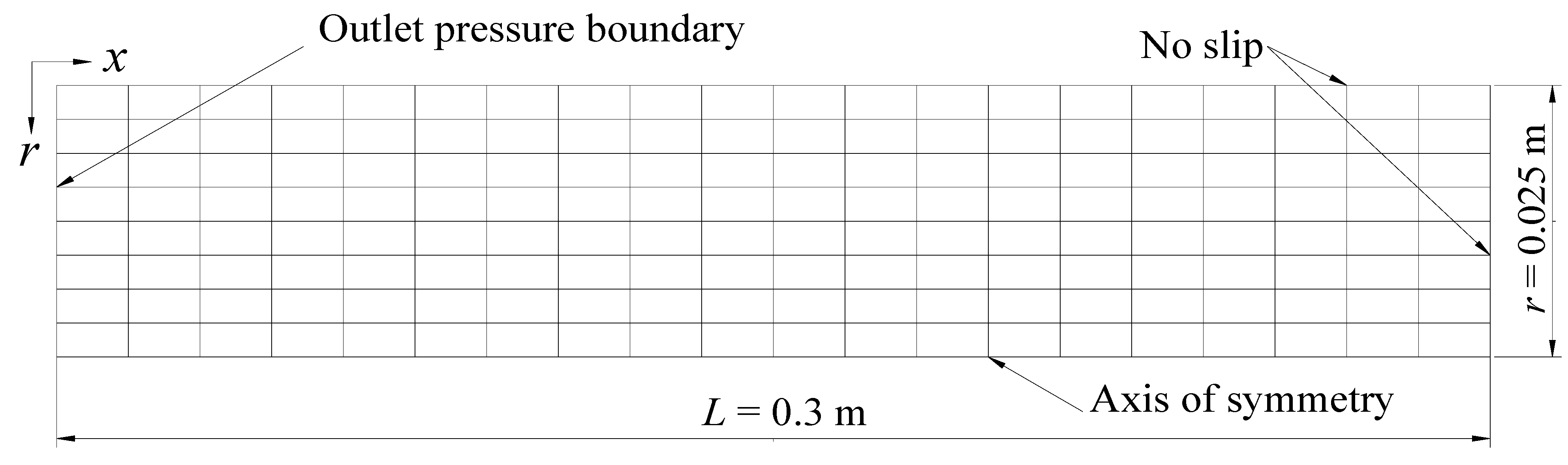
Many complex phenomenon are involved during the gas production process of hydrate dissociation by depressurization, which contains gas and water two-phase flow (mass transfer and transport), thermodynamic process and heat transfer (conduction, convection and phase change), and chemical reaction (the kinetic of hydrate dissociation). These information are all described in the above mathematical equations, which constitute a system of four coupled partial differential equations which are non-linearity and cannot be solved analytically (exactly). Several numerical examples have been tested to solve these equations [10,14,15,19,31,32,33,34,35]. In this work, the fully implicit simultaneous solution method combined with Newton’s iterative method is used to solve this model. The space and time derivatives of the equations were approximated by a block-centered finite difference scheme. The central difference approximation is used for the second order spatial derivatives and a backward difference is used for the first order time derivatives. After nonlinear partial differential equations are discretized into nonlinear algebraic equations, Newton-Raphson iteration method is used to linearize the fully implicit equations and these equations are solved simultaneously to obtain the solutions of pressure, temperature and saturation.

To verify the mathematical model and numerical solution, the numerical results are compared with the experimental data obtained by Masuda et al. [10]. The experiment and simulation conditions are summarized in Table 1. The Masuda et al.’s experiment was conducted using a Bereasandstone core sample with a cylindrical geometry, which is 0.3 m in length and 0.05 m in diameter. The intrinsic porosity and the intrinsic permeability are 0.182 md and 97.98 md, respectively. The core is initially saturated with hydrate, water and gas (S_h = 0.443, S_w = 0.206, and S_g = 0.351). The initial pressure and temperature are 3.75 MPa and 2.3 °C, respectively. The core sample is placed in a temperature bath with T_b = 2.3 °C. The pressure at the outlet located at the left of core sample is maintained at 2.84 MPa for depressurization. It was found that the maximum methane gas production could reach about 9048 cm³ under standard conditions (Scm³) in Masuda et al.’s experiment [10]. Figure 1 shows a two-dimensional computational domain for the laboratory-scale hydrate core, which is equally divided into 8 blocks in radial direction and 20 blocks in axial direction. The numerical simulation for analyzing the hydrate dissociation of an axisymmetric hydrate core was performed and the corresponding gas production behaviors were analyzed. The simulation results of the cumulative gas production and the variations of the temperature obtained using this 2-D depressurization-induced hydrate dissociation model were found to be good agreement with the experimental data [10]. The detail information for the validation of the model can be found in our previous literatures [34,35], which indicated that the mathematical model is capable of investigating the methane gas production behaviour of hydrate dissociation under the conditions of different depressurizing approaches.

Table 1. Primary physical variable values used in the hydrate depressurization model from the experimental study of Masuda et al. [10].

Core length, L (m)	0.3	Core diameter, D (m)	0.05
Core pressure, P0 (MPa)	3.75	Core temperature, T0 (°C)	2.3
Intrinsic porosity, Φ0	0.182	Intrinsic permeability, K0 (md)	97.98
Outlet pressure, Pp0 (MPa)	2.84	Bath temperature, Tb (°C)	2.3
Hydrate saturation, Sh	0.443	Water saturation, Sw	0.206
Gas saturation, Sg	0.351	Permeability reduction index, N	10

Table 1. Primary physical variable values used in the hydrate depressurization model from the experimental study of Masuda et al. [10].

Core length, L (m)	0.3	Core diameter, D (m)	0.05
Core pressure, P0 (MPa)	3.75	Core temperature, T0 (°C)	2.3
Intrinsic porosity, Φ0	0.182	Intrinsic permeability, K0 (md)	97.98
Outlet pressure, Pp0 (MPa)	2.84	Bath temperature, Tb (°C)	2.3
Hydrate saturation, Sh	0.443	Water saturation, Sw	0.206
Gas saturation, Sg	0.351	Permeability reduction index, N	10

4. Results and Discussion

In our work, the comparisons of gas production behaviors of hydrate dissociation with different depressurizing approaches are based on the same condition. The primary physical variable values used in different numerical simulations are the same and listed in Table 1. To achieve the different depressurizing approaches, the ideas from Li et al.’s paper [36] have been adopted in this mathematical modeling. The numerical results of gas production behaviors have been used to discuss the effects of different depressurizing ranges, different depressurizing rates and the combined depressurization mode of the both approaches.

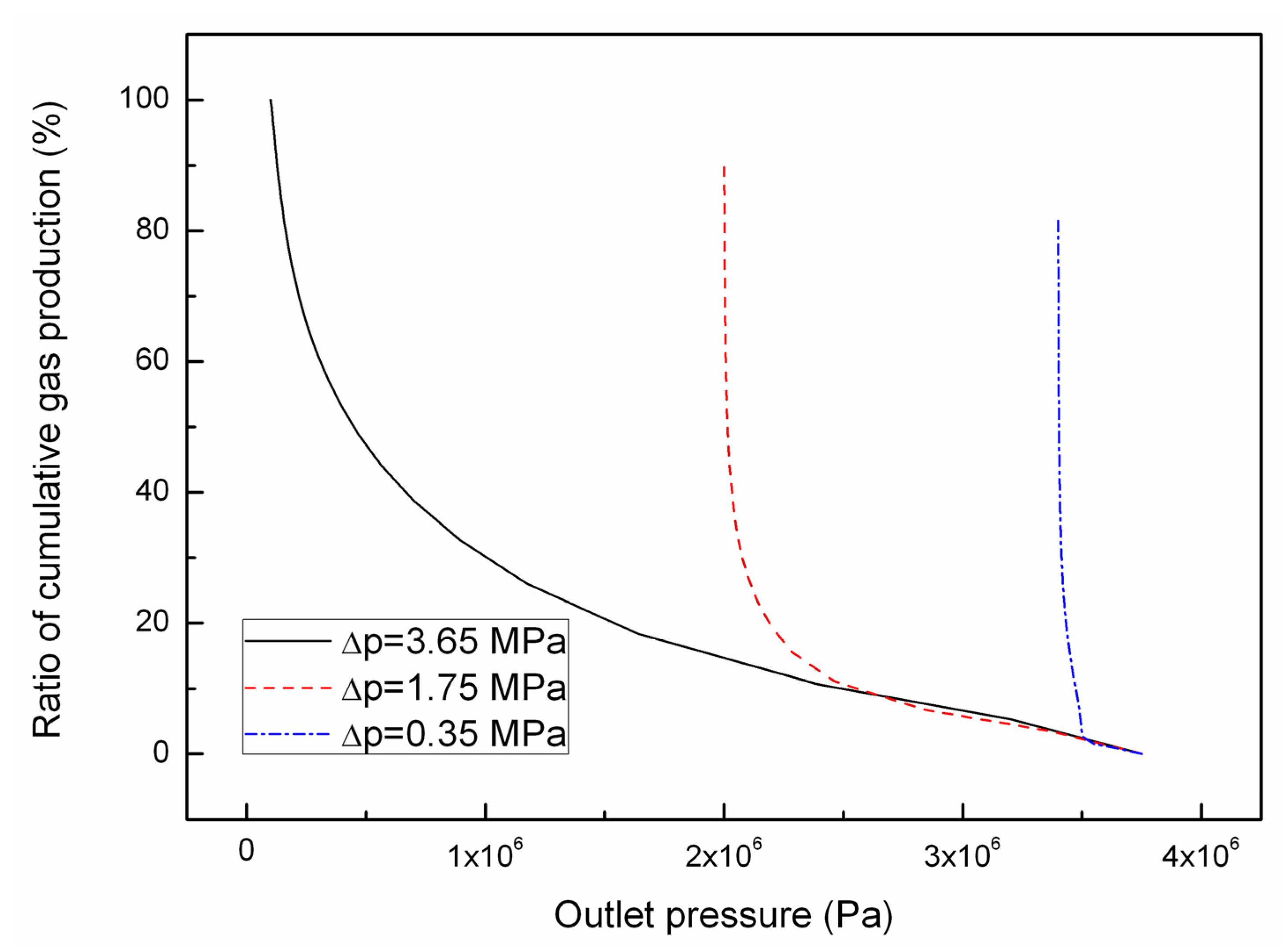
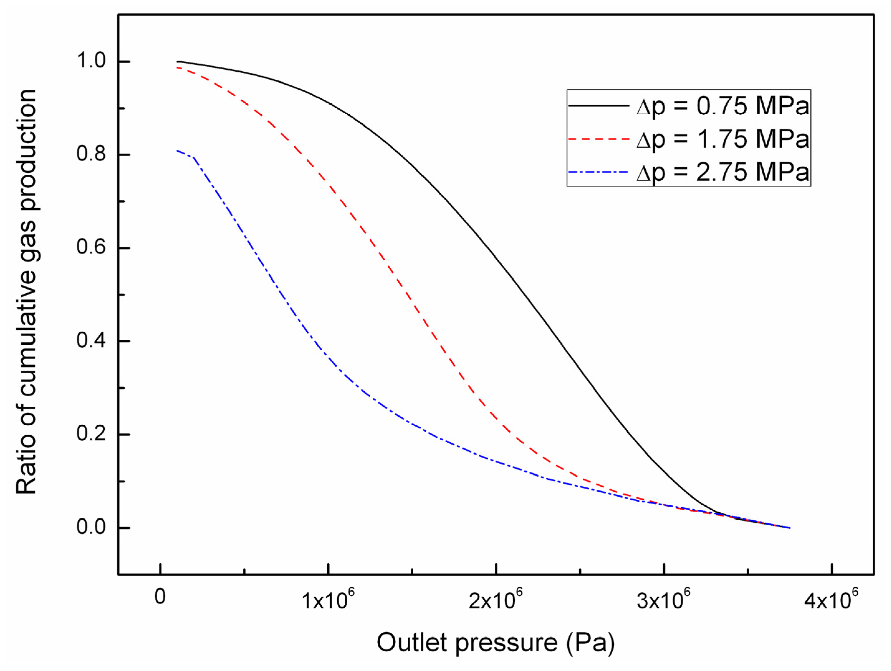
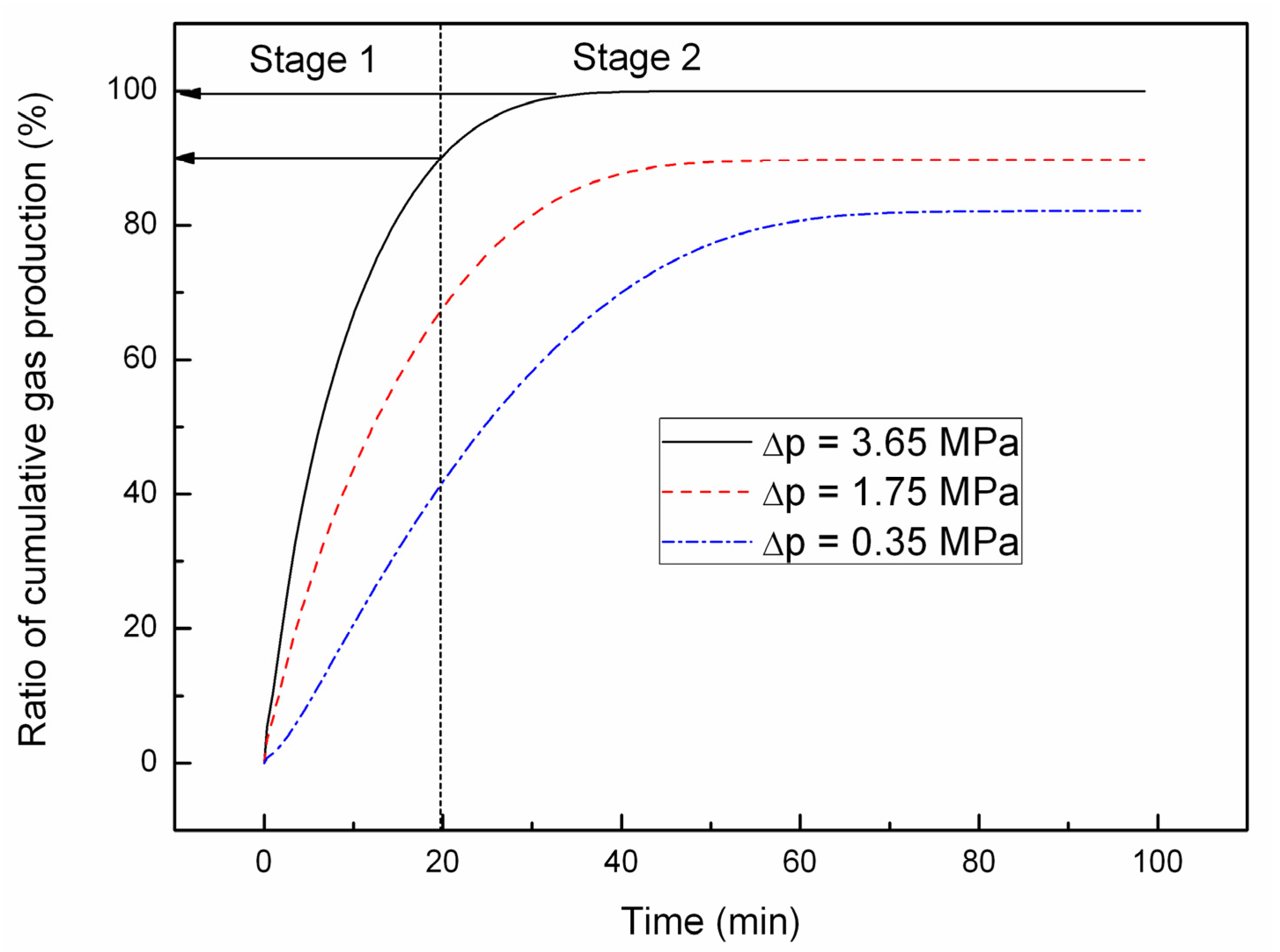
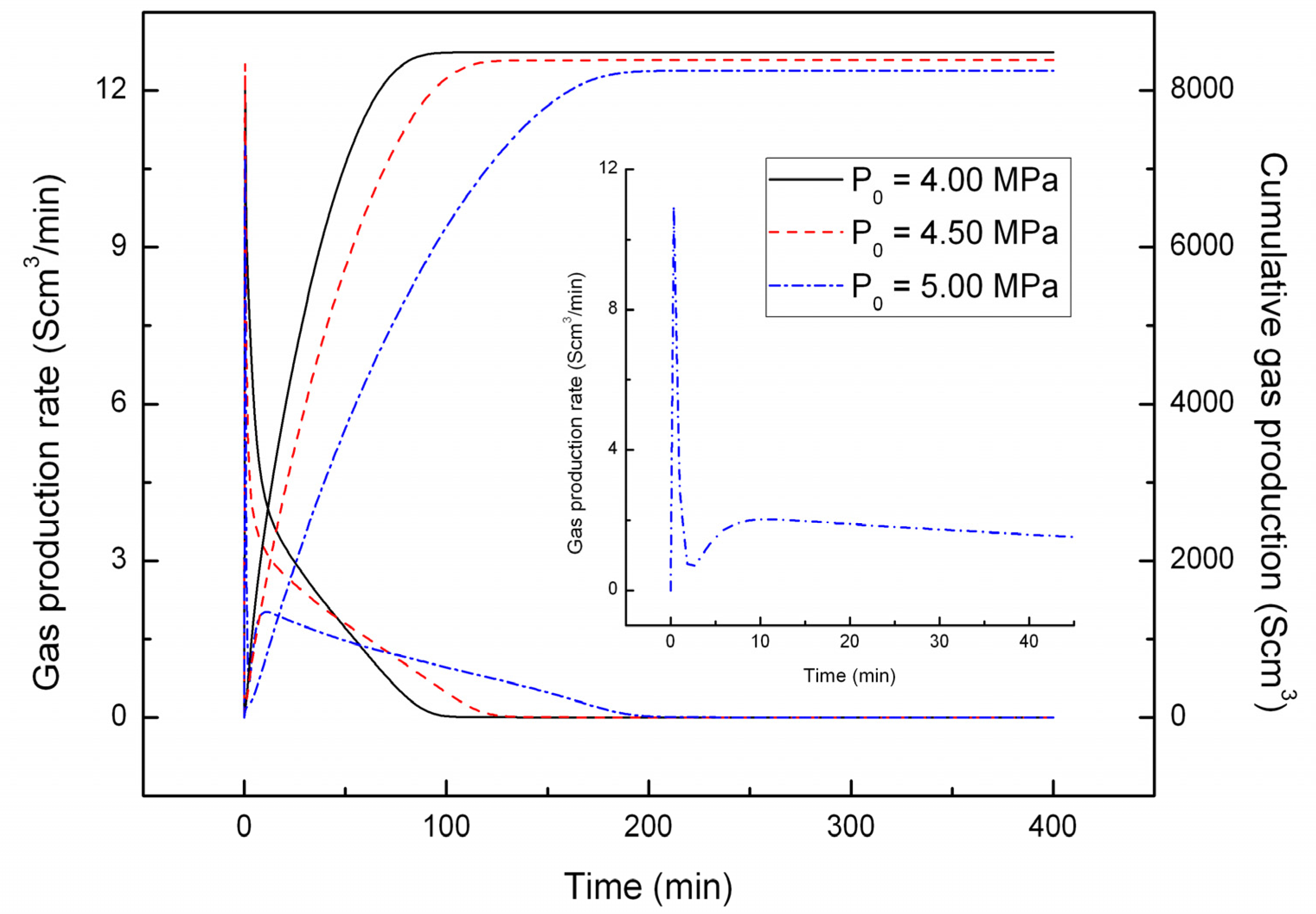
4.1. Effect of the Depressurizing Range

In this section, the effects of different depressurizing ranges ∆p (0.35 MPa, 1.75 MPa and 3.65 MPa) on the gas production from hydrate are studied. The initial pressure of the laboratory-scale hydrate system is fixed at P₀ = 3.75 MPa, corresponding to the values of different depressurizing ranges. Moreover, the outlet pressure is designed or set to 3.4 MPa, 2.0 MPa and 0.1 MPa, respectively. For the convenience of discussion, we define the percentage of cumulative gas production as the ratio of the cumulative gas production from hydrate dissociation and the maximum of gas production. Figure 2 shows the time evolutions of the percentage of cumulative gas production for different depressurizing ranges. As seen from this figure, the percentage of cumulative gas production increases more quickly with a larger ∆p. Based on Equation (6), a large driving force of pressure can lead to high gas productivity. As a result, more amount of cumulative gas can be produced with the higher depressurization range.

Figure 2. The percentage of cumulative gas production time evolution for different depressurizing ranges.

Figure 2. The percentage of cumulative gas production time evolution for different depressurizing ranges.

In addition, there are two stages for the cumulative gas production under the conditions of different depressurizing ranges as plotted in Figure 2. First, it becomes very high rapidly, in which the ascending segment corresponds to the almost amount of gas production from hydrate in the first stage (called stage 1, to distinguish another stage), then slows down gradually to stagnation at the end as shown in the stage 2. The change of the increase of gas production is due to the facts of the evolution of pressure difference and the ability of providing heat. During the early period of the depressurization, the heat for hydrate dissociation is abundant, a great pressure different is created between the outlet and the inner region once the pressure of outlet was decreased to a low value, by which the free gas and the gas generated from the dissociated hydrate are driven out, a vast amount of cumulative gas is produced in a short time. Whereas in the second stage the free gas and the latent heat of hydrate-bearing porous media are exhausted, the heat for hydrate incessant dissociation is poor and even needs to “borrow” additional heat from the ambient environment, and the decomposition of hydrate appears to be complete in some regions while only occurring in some small regions. All of the above lead to a reduction in the stage 2 of cumulative gas production.

To further discuss the impact of depressurizing range on gas production, the relationships between the percentage of cumulative gas production and outlet pressure for different depressurizing ranges are plotted in Figure 3. It can be observed that there is a similar tendency represented in the change of the cumulative gas production as the decreasing outlet pressure. First, the increase of cumulative gas production is slow, subsequently the gas production increases dramatically. The sharp increasing segments of the curves indicate that hydrate will begin to decompose massively once the system pressure decreases to the given outlet pressure.

Figure 3. The relationship between the percentage of cumulative gas production and outlet pressure for different depressurizing ranges.

Figure 3. The relationship between the percentage of cumulative gas production and outlet pressure for different depressurizing ranges.

Figure 4 shows the variation of gas production rate and cumulative gas production with initial pressure of gas hydrate system when the initial pressures are 4.00 MPa, 4.50 MPa and 5.00 MPa, respectively, and the depressurizing range for gas production is 2.0 MPa. We can see from Figure 4 that the gas production rate and cumulative gas production are lower with a higher initial pressure. However, the production lifetime becomes longer as the increase of initial pressure. This is due to the fact that we consider the effect of initial pressure on gas production rate with the condition of same depressurizing range. The system initial temperature is the same for the simulations, which implies that the phase equilibrium pressure of gas hydrate (P_e) is equivalent. For the high initial pressure, the gas hydrates do not dissociate before the system pressure lowers to P_e. So, the initial gas generated is only the free gas and flows in low permeability formation bearing gas hydrate, which causes the low gas production performance and delayed time that the gas generated from hydrate dissociation appears as the system pressure is reduced below the phase equilibrium pressure P_e. That is why there are two peaks presenting for the gas production rate of P₀ = 5.00 MPa, in which the first peak can be attributed to the free gas, and the second peak is due to the dissociated gas. On the contrary, under the low initial pressure, the pressure can be soon lowered to P_e. Therefore, the dissociated gas hydrate can supply an amount of gas and lead to the increase of permeability, which causes a high gas production behavior and the shorter time for stable production. For the field gas hydrate production, it can mean that a higher gas production is not associated with a higher initial reservoir pressure.

Figure 4. Gas production rate and cumulative gas production time evolution for different initial pressures with the same depressurizing range.

Figure 4. Gas production rate and cumulative gas production time evolution for different initial pressures with the same depressurizing range.

Considering the endothermic phenomena in gas hydrate dissociation process induced by depressurization, the ambient temperature (i.e., the heat transfer from environment) and thermal conductivity are taken into account for investigating the gas production with depressurizing ranges ∆p = 3.65 MPa. Gas production rate and cumulative gas production variation with different thermal conductivity conditions are shown in Figure 5.

Figure 5. Gas production rate and cumulative gas production time evolution for different thermal conductivity of the hydrate-bearing porous media with the same depressurizing ranges.

Figure 5. Gas production rate and cumulative gas production time evolution for different thermal conductivity of the hydrate-bearing porous media with the same depressurizing ranges.

The thermal conductivity of the hydrate-bearing porous media is 1.5 W/m·K, 4.0 W/m·K and 8.0 W/m·K, respectively. When the thermal conductivity increases, accordingly the gas production also increases as expected. It can be explained by a faster heat transfer to provide the needed dissociation heat. However, it is worth noting that the effects of higher thermal conductivity on the gas production behaviors seem negligible. This indicates that the heat transfer, one of three mechanisms for gas hydrate production by depressurization [37], has limited impact on hydrate dissociation for a low permeability hydrate-bearing porous media (K₀ = 97.98 md).

Figure 6 shows the variation of gas production rate and cumulative gas production under the conditions of different ambient temperatures with same depressurizing range (∆p = 3.65 MPa). The temperatures studied are 1.3 °C, 2.3 °C and 3.3 °C, while maintaining the thermal conductivity condition to be same λ = 1.5 W/m·K for all simulations. Compared to thermal conductivity, the ambient temperature has a significant influence on the gas production behavior as shown in Figure 6. A higher temperature leads to a better gas production performance in terms of both gas production rate and cumulative gas production. The maximum of gas production rate is 14.04 Scm³/min, 14.32 Scm³/min and 14.76 Scm³/min for T increasing from 1.3 °C to 3.3 °C, respectively. One of the reasons for this behavior is the capacity of substantial amount of heat provided to raise the temperature of the hydrate to the dissociation temperature. Furthermore, as expressed in Equations (6) and (7), the hydrate dissociation kinetic constant k_d and the driving force of hydrate dissociation are higher at higher temperature, causing a faster dissociation rate and the increase of cumulative gas produced. Therefore, it could suggest that the hydrate dissociation kinetics dominates the gas production process for a low permeability hydrate-bearing porous media, confirming the result of an earlier study [16].

Figure 6. Gas production rate and cumulative gas production time evolution for different temperature with the same depressurizing range.

Figure 6. Gas production rate and cumulative gas production time evolution for different temperature with the same depressurizing range.

In addition, the low temperature dramatically weakens the gas production behavior as the case of T = 1.3 °C shown in the Figure 6. For a low temperature to hydrate reservoir, if the depressurizing range is very large, massive dissociation of hydrate will occur thus causing the inner temperature of hydrate-bearing sediments to decrease more significantly, even below the freezing point of water. Hence, large depressurizing range maybe unfavorable for the exploitation in the field-scale hydrate reservoir.

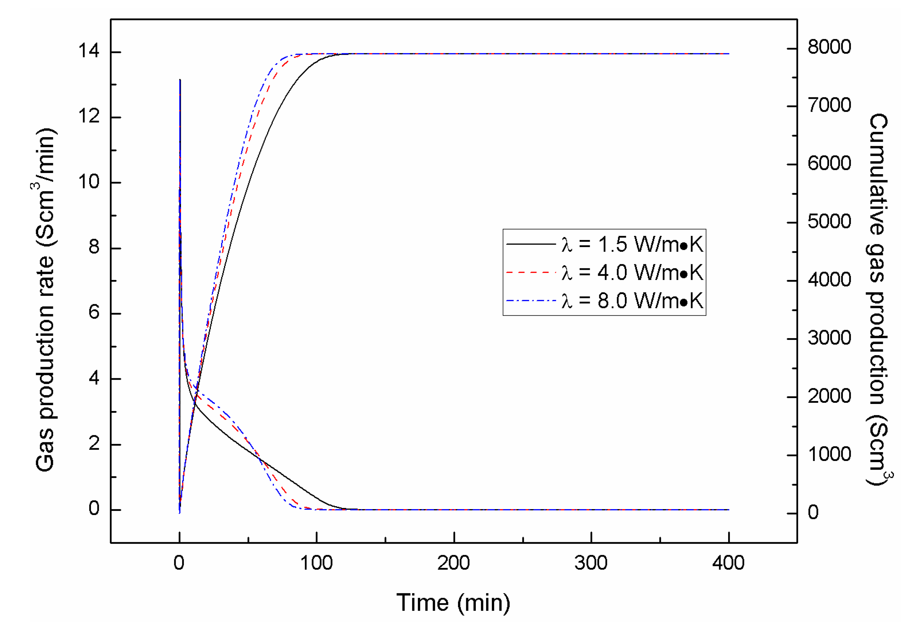
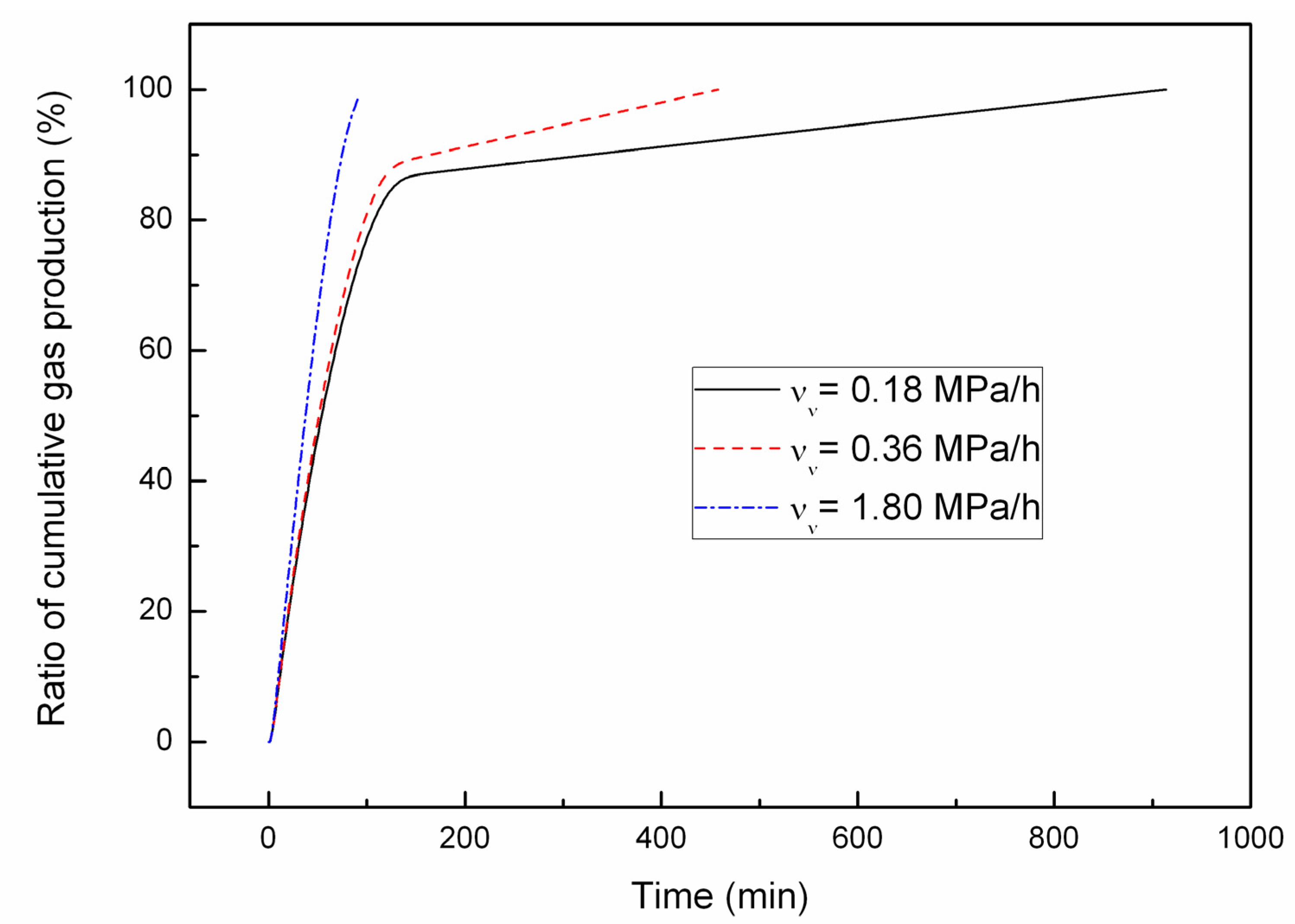
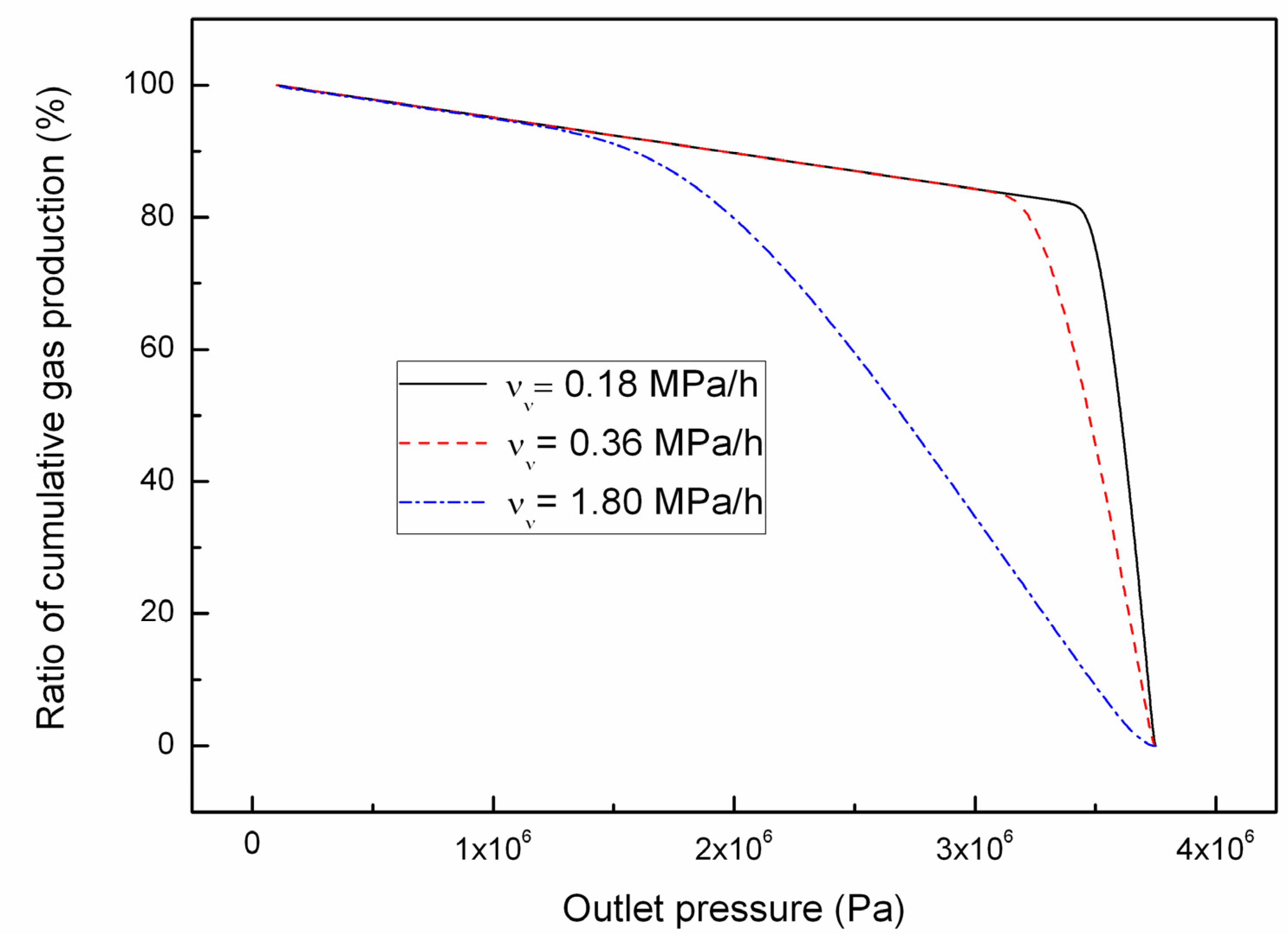
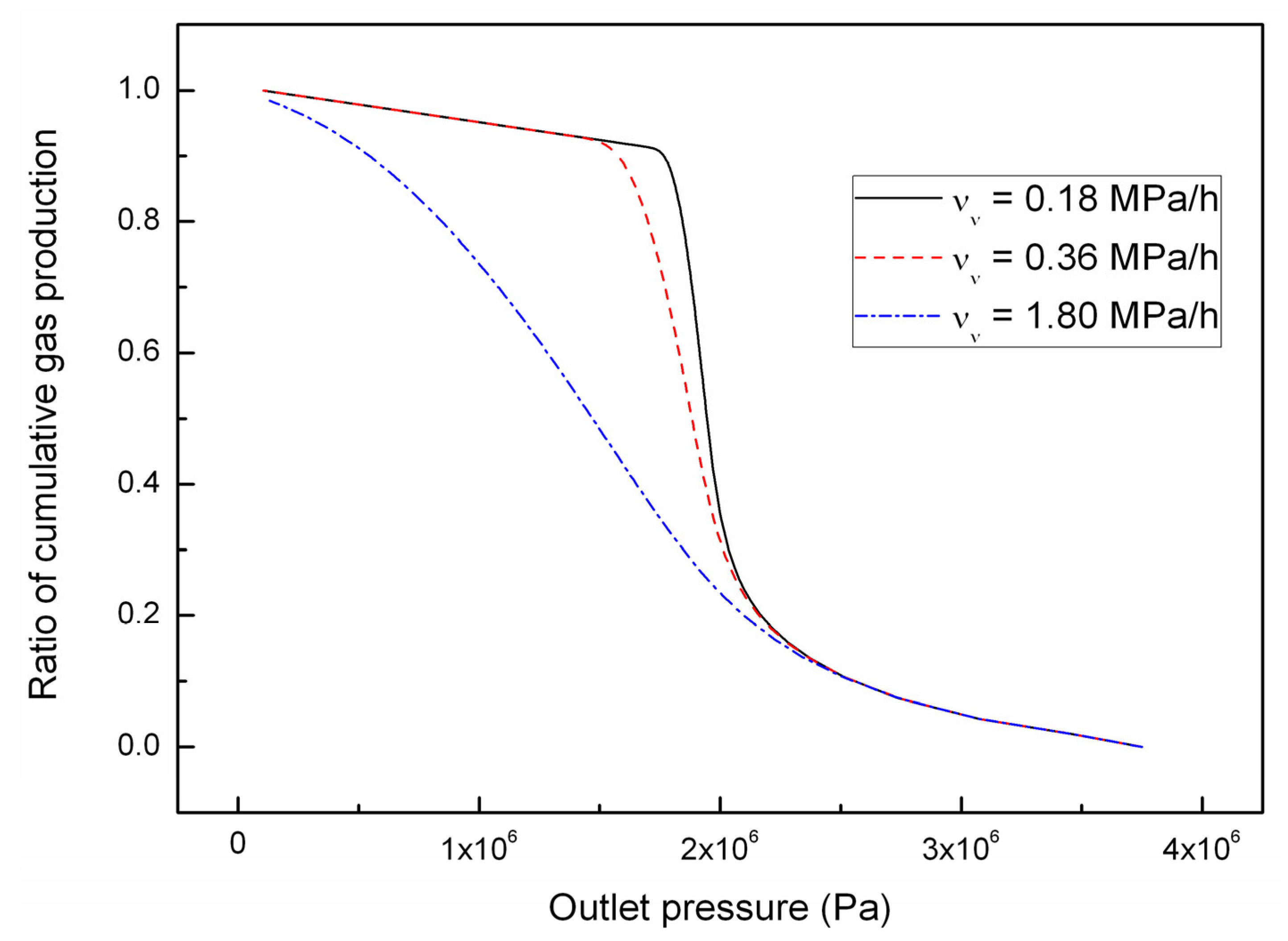
4.2. Effect of the Depressurizing Rate

As an alternative exploitation scenario, the depressurizing rate is conducted by the means of decreasing the pressure at a certain rate, but not setting to a low constant outlet pressure. In this section, simulations with different depressurizing rates ν_ν of 0.18 MPa/h, 0.36 MPa/h and 1.80 MPa/h are performed to investigate the effect of the depressurizing rate on the gas production from hydrate. The initial pressure of the laboratory-scale hydrate system is fixed at P₀ = 3.75 MPa, then the pressure is reduced to atmospheric pressure (1.0133 × 10⁵ Pa) with different depressurizing rates. Figure 7 represents the time evolutions for percentage of cumulative gas production with different depressurizing rates. It can be found that the different depressurizing rate only affects the production lifetime rather than the finial gas production, and the time of gas production becomes shorter with the increase of depressurizing rate ν_ν, which is different from the case of depressurizing range as already discussed in Figure 2. The reason for this is that the higher depressurizing rate leads to a faster depressurization and hydrate dissociation earlier in the production process. Moreover, there also are two stages for the cumulative gas production under the conditions of different depressurizing rates as indicated in Figure 7, which is similar to the case of depressurizing range.

Figure 7. The percentage of cumulative gas production time evolution for different depressurizing rates.

Figure 7. The percentage of cumulative gas production time evolution for different depressurizing rates.

In Figure 8, the relationships between the percentage of cumulative gas production and outlet pressure for different depressurizing rates are shown. In the initial period of the production process, the cumulative gas production drastically increases with a decreasing outlet pressure for each case of depressurizing rate, which indicates that the massive gas hydrates begin to dissociate when the pressure lowers to the phase equilibrium pressure (P_e = 3.68 MPa at T = 2.3 °C). While the effect of low pressure to gas production will be weakened as the hydrate disappears gradually. Finally, the cumulative gas production reaches a same maximum for all the cases. In addition, the cumulative gas production as indicated in Figure 8 decreases with an increase of depressurizing rate ν_ν for the same depressurizing range, which is clear especially in the early stages of hydrate depressurization process. When the outlet pressure is reduced to 3.5 MPa, the percentage of cumulative gas production is 75.05%, 44.77% and 8.53%, respectively, for ν_ν = 0.18 MPa/h, 0.36 MPa/h and 1.80 MPa/h. This numerical result suggested that more amount of gas production can be produced from field hydrate reservoir with lowering the depressurizing rate for a certain depressurizing range.

Figure 8. The relationships between the percentage of cumulative gas production and outlet pressure for different depressurizing rates.

Figure 8. The relationships between the percentage of cumulative gas production and outlet pressure for different depressurizing rates.

Figure 9 shows the variation of gas production rate and cumulative gas production at different ambient temperature and thermal conductivity cases with the same depressurizing rate (ν_ν = 1.80 MPa/h). Whether the ambient temperature decreases from 5.3 °C to 0.3 °C or thermal conductivity is reduced from 4.0 W/m·K to 1.5 W/m·K, the corresponding reduction in the volume of the produced gas appears with expectations. The reasons for this are already discussed above for Figure 5 and Figure 6. On the whole, higher ambient temperature and higher thermal conductivity are favorable for more gas production. However, note that Figure 9 also indicates that, in the initial period of the production process, the gas production behavior mainly depends on the ambient temperature. The gas production increases with the increasing ambient temperature, but varies little with thermal conductivity λ of hydrate-bearing porous media. After a period of production time, the effect of λ on gas production is even dominant from approximate 50 min to the end of the production periods comparing with the case of different ambient temperature. In other words, the hydrate dissociation kinetics (indicated by ambient temperature) is important for the initial production process of a laboratory-scale hydrate core, while the heat transfer (displayed by thermal conductivity) dominates the later period of production process.

Figure 9. Gas production rate and cumulative gas production time evolution for different temperature and rock thermal conductivity with the same depressurizing rate.

Figure 9. Gas production rate and cumulative gas production time evolution for different temperature and rock thermal conductivity with the same depressurizing rate.

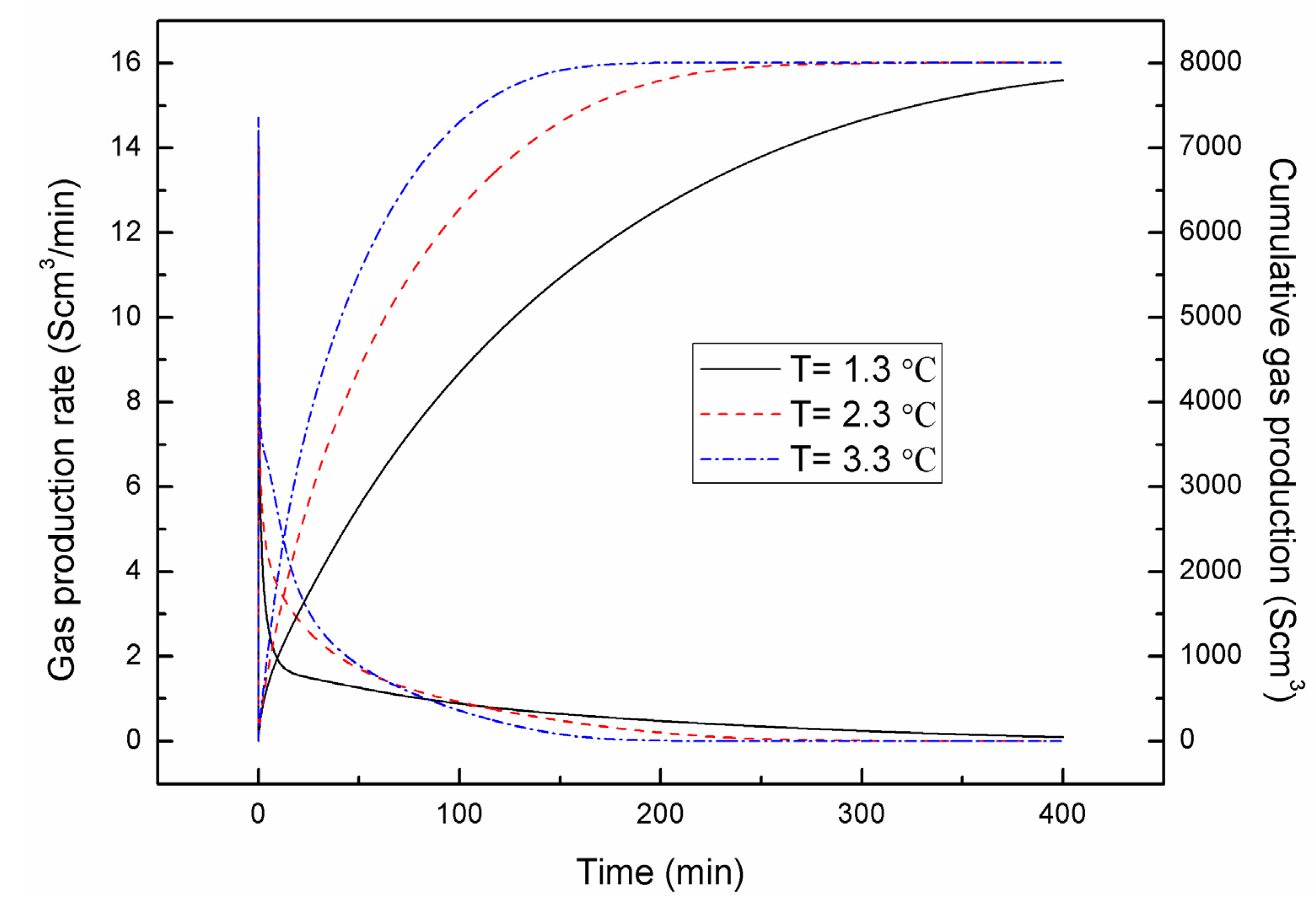
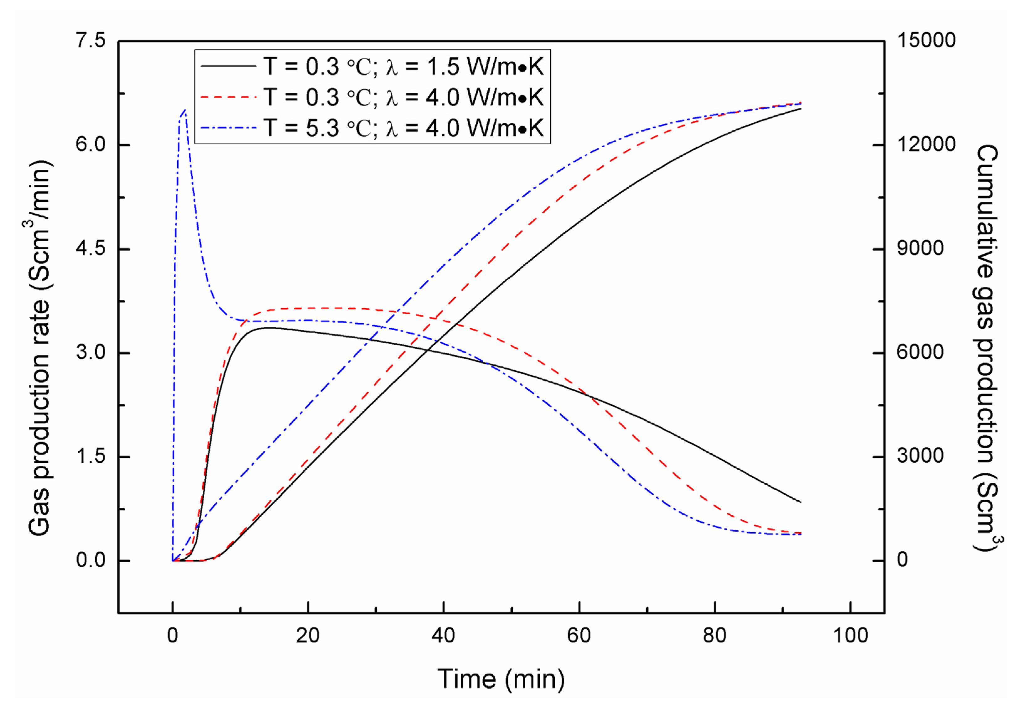
4.3. Effect of Combined Depressurization Approach

In this section, the effects of the combination of both depressurizing range and depressurizing rate on gas production are investigated. Two kinds of combination of depressurization approach have been proposed. The first kind of combination (called Class 1 in the following discussion) is that different depressurizing ranges are adopted in the initial period of the gas production process, when the pressure is reduced to the corresponding value of depressurization process at the different depressurizing range, the simulations are conducted at a certain depressurizing rate until the pressure reaches the atmospheric pressure. The second kind of combination (called Class 2 in the following discussion) is that the simulations are performed at a same depressurizing range initially, then to continue the depressurization of the gas production process with different depressurizing rates and complete at the atmospheric pressure. The other simulation conditions maintain the same as listed in Table 1. Figure 10 and Figure 11 show the relationships between the percentage of cumulative gas production and outlet pressure for the Class 1 and Class 2 of combined depressurization modes, respectively.

For the Class 1 of combined depressurization mode, the initial depressurization process is implemented with different depressurizing range ∆p from 0.75 MPa to 2.75 MPa, and the later depressurization process takes place with a constant depressurizing rate (ν_ν = 1.80 MPa/h). As shown in Figure 10, the initial larger depressurizing range leads to a lower gas production performance during the mostly depressurization process and even the case of ∆p = 2.75 MPa, ν_ν = 1.80 MPa/h results in a low final cumulative gas production (only over 80%). For the Class 2 of combined depressurization mode, as previously stated that the pressure is firstly reduced by the same depressurizing range (∆p = 1.75 MPa) and then decreases with different depressurizing rates (ν_ν = 0.18 MPa/h, 0.36 MPa/h and 1.80 MPa/h), the variation of gas production with the outlet pressure is much simpler and similar to the case of single depressurization process with the depressurizing rate. The curves of the Class 1 and Class 2 have the feature of “concave” line as indicated in the case of depressurizing range (Figure 3), and meanwhile have the characteristic of “convex” line presented in the case of depressurizing rate (Figure 8). Additionally, in Figure 10, the case represented by red dashed line is the same as the case shown in Figure 11 by a blue dash-dot line, i.e., the first depressurization process is with a depressurizing range ∆p = 1.75 MPa, and the next depressurization process is with a depressurizing rate ν_ν = 1.80 MPa/h. Therefore, it can be known that the Class 2 of combined depressurization mode is much superior to the Class 1 of combined depressurization mode for a long and stable gas production process through the comparison with Figure 10 and Figure 11.

Figure 10. The relationships between the percentage of cumulative gas production and outlet pressure for the Class 1 of combined depressurization mode.

Figure 10. The relationships between the percentage of cumulative gas production and outlet pressure for the Class 1 of combined depressurization mode.

Figure 11. The relationships between the percentage of cumulative gas production and outlet pressure for the Class 2 of combined depressurization mode.

Figure 11. The relationships between the percentage of cumulative gas production and outlet pressure for the Class 2 of combined depressurization mode.

5. Conclusions

In this paper, a 2D axisymmetric model for simulating the gas production from hydrate by depressurization is developed. Based on the model, the gas production behaviors were analyzed under different depressurizing approaches. From the numerical simulation results, the following conclusions can be drawn:

(1) The depressurizing range has significant influence on the final gas production. The amount of cumulative gas increases with an increase in the depressurization range.

(2) The depressurizing rate only affects the production lifetime rather than the final gas production. The time of gas production decreases with the increase of depressurizing rate. Moreover, the simulations also suggested that more amount of gas production can be produced from field hydrate reservoir with lowering the depressurizing rate for a certain depressurizing range, especially in the initial stage of hydrate depressurization.

(3) The parameter analysis of initial pressure with the same large depressurization range to gas production indicated that the gas production performance decreases and the period of stable production increases with the increasing initial pressure.

(4) For the case of depressurizing range, the numerical results in the analysis of thermal conductivity of the hydrate-bearing porous media to gas production indicated that the effect of thermal conductivity on gas production performance can be negligible. Moreover, the results also suggested that the heat transfer has limited impact on hydrate dissociation for a low permeability hydrate-bearing porous media.

(5) Under a given depressurizing range, the higher ambient temperature for gas hydrate production, the better gas production performance in terms of both gas production rate and cumulative gas production.

(6) In the case of depressurizing rate, the numerical results showed that the gas production is controlled by the ambient temperature and thermal conductivity in different period of production process.

(7) In the case of combined depressurization mode, the Class 2 is much superior to the Class 1 for a long and stable gas production process.

References

1. Sloan, E.D. Clathrate Hydrates of Natural Gas, 2nd ed.; Marcel Dekker Inc: New York, NY, USA, 1998. [Google Scholar]
2. Max, M.D.; Dillon, W.P. Oceanic methane hydrate: Character of the Blake Ridge hydrate stability zone and potential for methane extraction. J. Pet. Geol. 1998, 21, 343–358. [Google Scholar] [CrossRef]
3. Konno, Y.; Oyama, H.; Nagao, J.; Masuda, Y.; Kurihara, M. Numerical analysis of the dissociation experiment of naturally occurring gas hydrate in sediment cores obtained at the Eastern Nankai Trough, Japan. Energy Fuels 2010, 24, 6353–6358. [Google Scholar] [CrossRef]
4. Kumar, A.; Maini, B.; Bishnoi, P.R.; Clarke, M.; Zatsepina, O.; Srinivasan, S. Experimental determination of permeability in the presence of hydrates and its effect on the dissociation characteristics of gas hydrates in porous media. J. Pet. Sci. Eng. 2010, 70, 114–122. [Google Scholar] [CrossRef]
5. Khataniar, S.; Kamath, V.A.; Omenihu, S.D.; Patil, S.H.; Dandekar, A.Y. Modelling and economic analysis of gas production from hydrates by depressurization method. Can. J. Chem. Eng. 2002, 80, 135–143. [Google Scholar] [CrossRef]
6. Makogon, Y.F. Hydrates of Natural Gas, 1st ed.; Penn Well Publishing Company: Tulsa, OK, USA, 1997. [Google Scholar]
7. Pooladi-Darvish, M.; Zatsepina, O.; Hong, H.F. Behaviour of Gas Production from Type III Hydrate Reservoirs. In Proceedings of the 6th International Conference on Gas Hydrates (ICGH 2008), Vancouver, Canada, 6–10 July 2008.
8. Yousif, M.H.; Abass, H.H.; Selim, M.S.; Sloan, E.D. Experimental and theoretical investigation of methane-gas-hydrate dissociation in porous media. SPE Reserv. Eng. 1991, 6, 69–76. [Google Scholar] [CrossRef]
9. Kim, H.; Bishnoi, P.R.; Heidemann, R.A.; Rizvi, S. Kinetics of methane hydrate decomposition. Chem. Eng. Sci. 1987, 42, 1645–1653. [Google Scholar] [CrossRef]
10. Masuda, Y.; Fujinaga, Y.; Naganawa, S.; Fujita, K.; Sato, K.; Hayashi, Y. Modeling and Experimental Studies on Dissociation of Methane Gas Hydrates in Bereasandstone Cores. In Proceedings of the 3rd International Conference on Gas Hydrates, Salt Lake City, UT, USA, 8–12 July 1999.
11. Ji, C.; Ahmadi, G.; Smith, D.H. Natural gas production from hydrate decomposition by depressurization. Chem. Eng. Sci. 2001, 56, 5801–5814. [Google Scholar] [CrossRef]
12. Ji, C.; Ahmadi, G.; Smith, D.H. Constant rate natural gas production from a well in a hydrate reservoir. Energy Convers. Manag. 2003, 44, 2403–2423. [Google Scholar] [CrossRef]
13. Sun, X.; Mohanty, K.K. 1-D modeling of hydrate depressurization in porous media. Transp. Porous Media 2005, 58, 315–338. [Google Scholar] [CrossRef]
14. Sun, X.; Mohanty, K.K. Kinetic simulation of methane hydrate formation and dissociation in porous media. Chem. Eng. Sci. 2006, 61, 3476–3495. [Google Scholar] [CrossRef]
15. Moridis, G.J.; Kowalsky, M.B.; Pruess, K. TOUGH-Fx/HYDRATE V1.0.1 User’s Manual: A Code for the Simulation of System Behavior in Hydrate-Bearing Geological Media; Lawrence Berkeley National Laboratory: Berkeley, CA, USA, 2005; LBNL/PUB 3185. [Google Scholar]
16. Tang, L.G.; Li, X.S.; Feng, Z.P.; Li, G.; Fan, S.S. Control mechanisms for gas hydrate production by depressurization in different scale hydrate reservoirs. Energy Fuels 2007, 21, 227–233. [Google Scholar] [CrossRef]
17. Konno, Y.; Masuda, Y.; Hariguchi, Y.; Kurihara, M.; Ouchi, H. Key factors for depressurization-induced gas production from oceanic methane hydrates. Energy Fuels 2010, 24, 1736–1744. [Google Scholar] [CrossRef]
18. Liu, Y.; Strumendo, M.; Arastoopour, H. Simulation of methane production from hydrates by depressurization and thermal stimulation. Ind. Eng. Chem. Res. 2009, 48, 2451–2464. [Google Scholar] [CrossRef]
19. Gamwo, I.K.; Liu, Y. Mathematical modeling and numerical simulation of methane production in a hydrate reservoir. Ind. Eng. Chem. Res. 2010, 49, 5231–5245. [Google Scholar] [CrossRef]
20. Hyodo, M.; Nakata, Y.; Yoshimoto, N.; Ebinuma, T. Basic research on the mechanical behavior of methane hydrate-sediments mixture. Soils Found. 2005, 45, 75–85. [Google Scholar] [CrossRef]
21. Winters, W.J.; Waite, W.F.; Mason, D.H.; Gilbert, L.Y.; Pecher, I.A. Methane gas hydrate effect on sediment acoustic and strength properties. J. Pet. Sci. Eng. 2007, 56, 127–135. [Google Scholar] [CrossRef]
22. Masui, A.; Miyazaki, K.; Haneda, H.; Ogata, Y.; Aoki, K. Mechanical Characteristics of Natural and Artificial Gas Hydrate Bearing Sediments. In Proceedings of the 6th International Conference on Gas Hydrates (ICGH 2008), Vancouver, Canada, 6–10 July 2008.
23. Miyazaki, K.; Masui, A.; Tenma, N.; Ogata, Y.; Aoki, K. Study on mechanical behavior for methane hydrate sediment based on constant strain-rate test and unloading-reloading test under triaxial compression. Int. J. Offshore Polar Eng. 2010, 20, 61–67. [Google Scholar]
24. Li, Y.; Song, Y.; Yu, F.; Liu, W.; Zhao, J. Experimental study on mechanical properties of gas hydrate-bearing sediments using kaolin clay. China Ocean Eng. 2011, 25, 113–122. [Google Scholar] [CrossRef]
25. Li, Y.; Song, Y.; Liu, W.; Yu, F. Experimental research on the mechanical properties of methane hydrate-ice mixtures. Energies 2012, 5, 181–192. [Google Scholar] [CrossRef]
26. Klar, A.; Soga, K. Coupled Deformation-Flow Analysis for Methane Hydrate Production by Depressurized Wells. In Proceedings of the 3rd Biot Conference on Poromechanics, Norman, OK, USA, 24–27 May 2005.
27. Rutqvist, J.; Moridis, G. Numerical Studies of Geomechanical Stability of Hydrate-Bearing Sediments. In Proceedings of 2007 Offshore Technology Conference (OTC-18860), Houston, TX, USA, 30 April–3 May 2007.
28. Kimoto, S.; Oka, F.; Fushita, T. A chemo-thermo-mechanically coupled analysis of ground deformation induced by gas hydrate dissociation. Int. J. Mech. Sci. 2010, 52, 365–376. [Google Scholar] [CrossRef]
29. Selim, M.S.; Sloan, E.D. Heat and mass transfer during the dissociation of hydrate in porous media. AIChE J. 1989, 35, 1049–1052. [Google Scholar] [CrossRef]
30. Tester, J.W. Thermodynamics and Its Applications; Prentice Hall: Upper Saddle River, NJ, USA, 1997. [Google Scholar]
31. Hong, H.; Pooladi-Darvish, M. Simulation of depressurization for gas production from gas hydrate reservoirs. J. Can. Pet. Technol. 2005, 44, 39–46. [Google Scholar] [CrossRef]
32. Song, Y.; Liang, H. 2-D Numerical simulation of natural gas hydrate decomposition through depressurization by fully implicit method. China Ocean Eng. 2009, 23, 529–542. [Google Scholar]
33. Bai, Y.; Li, Q.; Li, X.; Du, Y. Numerical simulation on gas production from a hydrate reservoir underlain by a free gas zone. Chin. Sci. Bull. 2009, 54, 865–872. [Google Scholar] [CrossRef]
34. Liang, H.; Song, Y.; Chen, Y. Numerical simulation for laboratory-scale methane hydrate dissociation by depressurization. Energy Conver. Manag. 2010, 51, 1883–1890. [Google Scholar] [CrossRef]
35. Ruan, X.; Song, Y.; Liang, H.; Yang, M.; Dou, B. Numerical simulation of the gas production behavior of hydrate dissociation by depressurization in hydrate-bearing porous medium. Energy Fuels 2012. [Google Scholar] [CrossRef]
36. Li, S.; Chen, Y.; Hao, Y.; Du, Q. Experimental research on influence factors of natural gas hydrate production by depressurizing in porous media. J. China Univ. Pet. 2007, 31, 56–59. (in Chinese). [Google Scholar]
37. Hong, H.; Pooladi-Darvish, M. A Numerical Study on Gas Production from Formations Containing Gas Hydrates. In Proceedings of Canadian International Petroleum Conference, Calgary, Canada, 12–14 June 2003.