Optimization of Steam Pressure Levels in a Total Site Using a Thermoeconomic Method

Abstract
:1. Introduction
2. Model Representation
2.1. Transshipment Model of a Steam Network
2.2. Exergoeonomics
2.2.1. SPECO Method
2.2.2. Auxiliary Equations
3. Optimization of Network
3.1. Constraints
3.2. Decision Variables
4. Case Studies
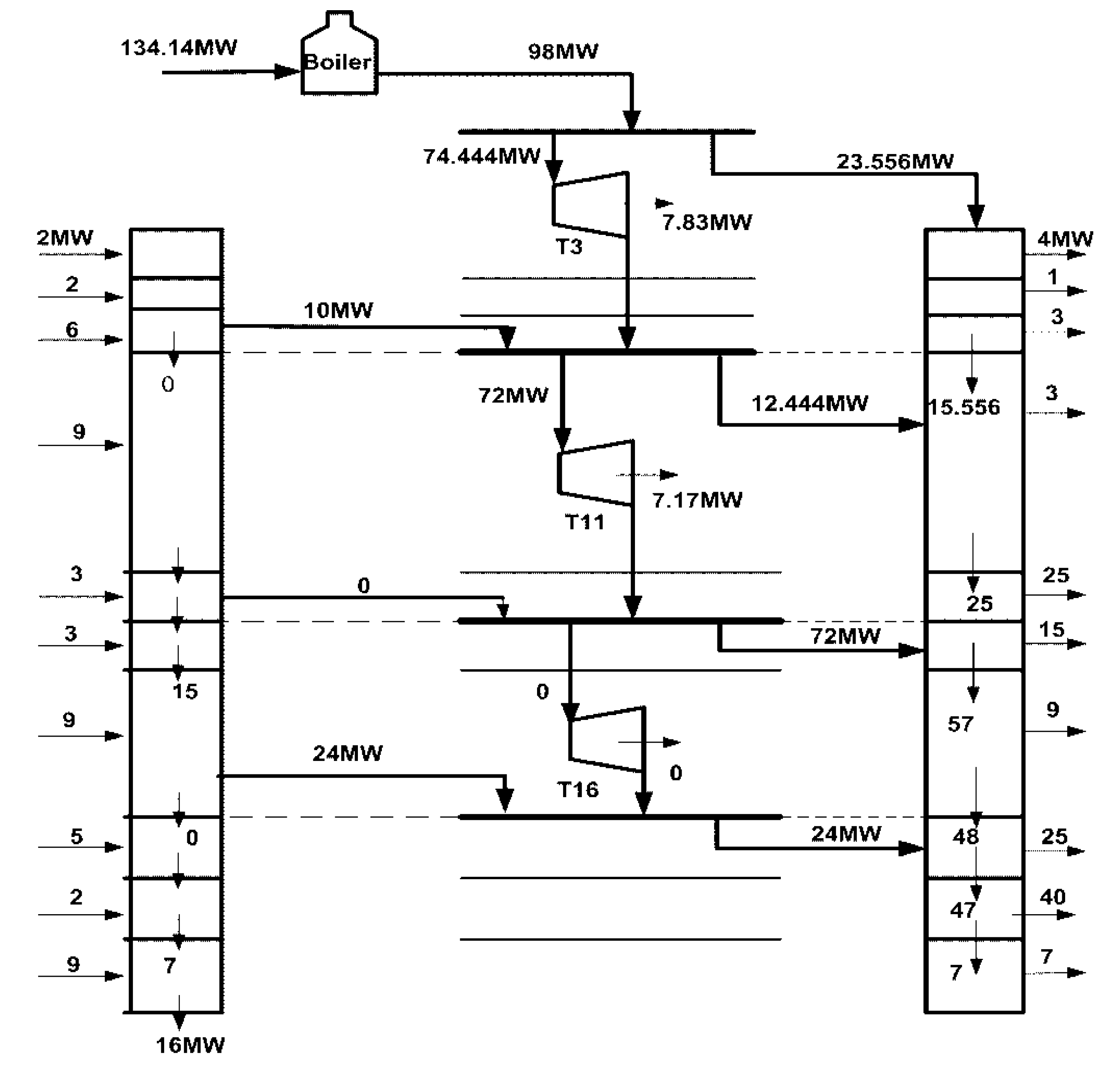
4.1. Case Study 1
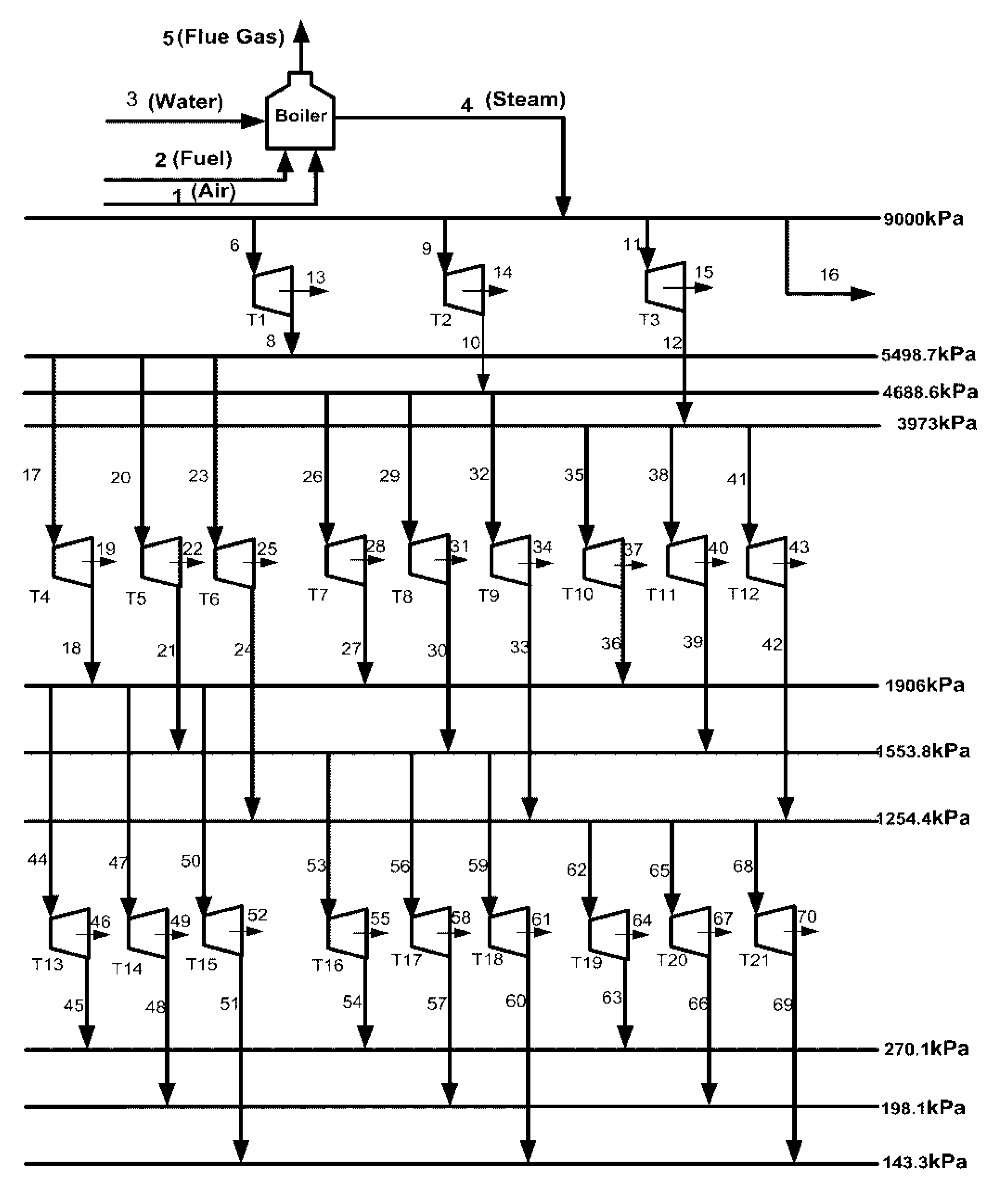
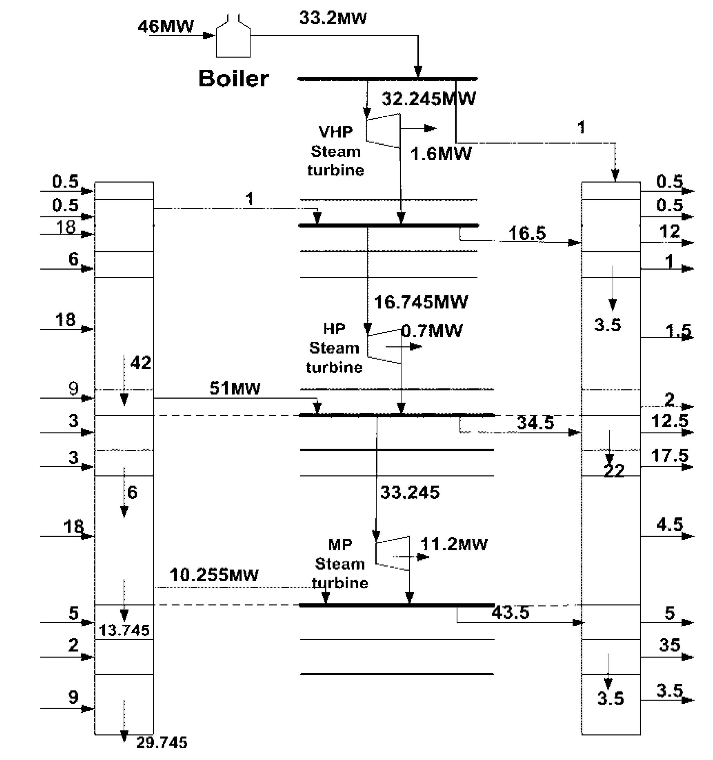
4.1.1. Definition of Problem and Superstructure

| Heat Provided (MW) | Heat Required (MW) | Interval (i,j) | Pressure Steam Level (kPa) |
|---|---|---|---|
| 12 | 1 | (1,1) | 5498.7 |
| 2 | 3 | (1,2) | 4688.6 |
| 6 | 20 | (1,3) | 3973 |
| 9 | 8 | (2,1) | 1906.3 |
| 3 | 0.8 | (2,2) | 1553.8 |
| 10 | 9 | (2,3) | 1254.4 |
| 9 | 3 | (3,1) | 270.1 |
| 5 | 40 | (3,2) | 198.5 |
| 2 | 7 | (3,3) | 143.3 |

4.1.2. Derivation of Constraints
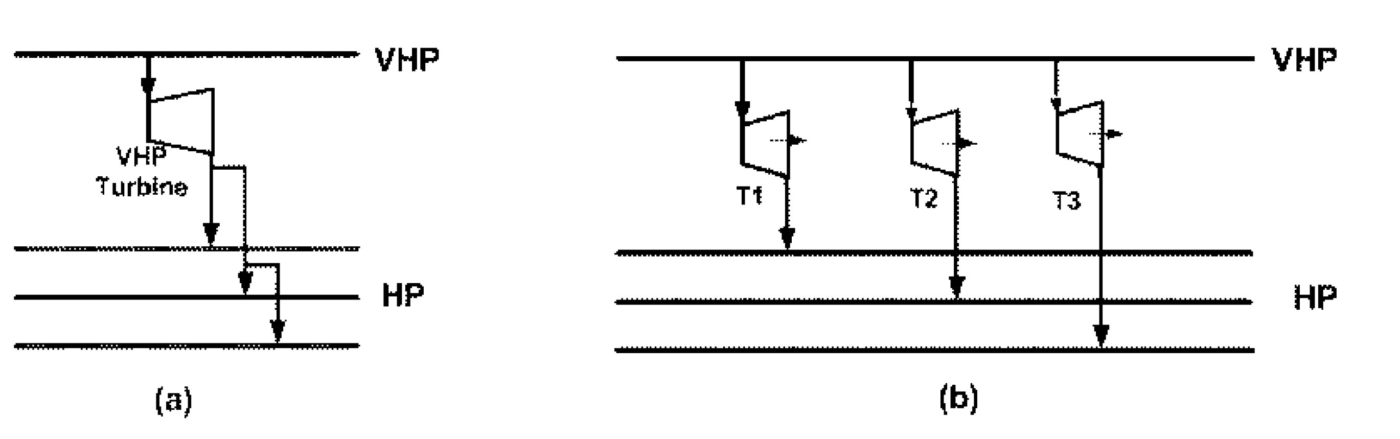
4.1.2.1. Steam Turbine
4.1.2.2. Boiler
4.1.2.3. Energy Balance of Steam Levels
4.1.2.4. Energy Balance of Temperature Intervals
4.1.2.5. Exergy and Cost Equations
4.1.3. Objective Function
4.1.4. Assumptions
- Exergy costs of entering air and water to the boiler are negligible.
- Exergy losses in all components are negligible.
- Steam has no chemical exergy.
- All condensates are returned to the boiler (no condensate losses and no blow down).
- Maintenance costs of the components are not accounted for.
- Boiler utilizes natural gas with Heat Value (HV) of 13,856 kWh/t as fuel. The price of natural gas and cooling water with ∆T = 20 °C is as 223 USD/t and 0.005 USD/t, respectively. The price of electricity is assumed as 0.12 USD/kWh.
- Investment costs (USD) of the boiler () and steam turbine () are according to Equation (30) and Equation (31) in which and are mass flow rate of steam (kg/s) and power output (kW), respectively:Equations (30) and (31) were obtained from the regression process based on the data reported by the website of Equip Cost [17] and Loh et al. [18], respectively.
- Marshall and Swift equipment cost index for the process industries in the first quarter of 2011 is 1549.8 [19].
- Annual system operation time at nominal capacity is 7008 hours.
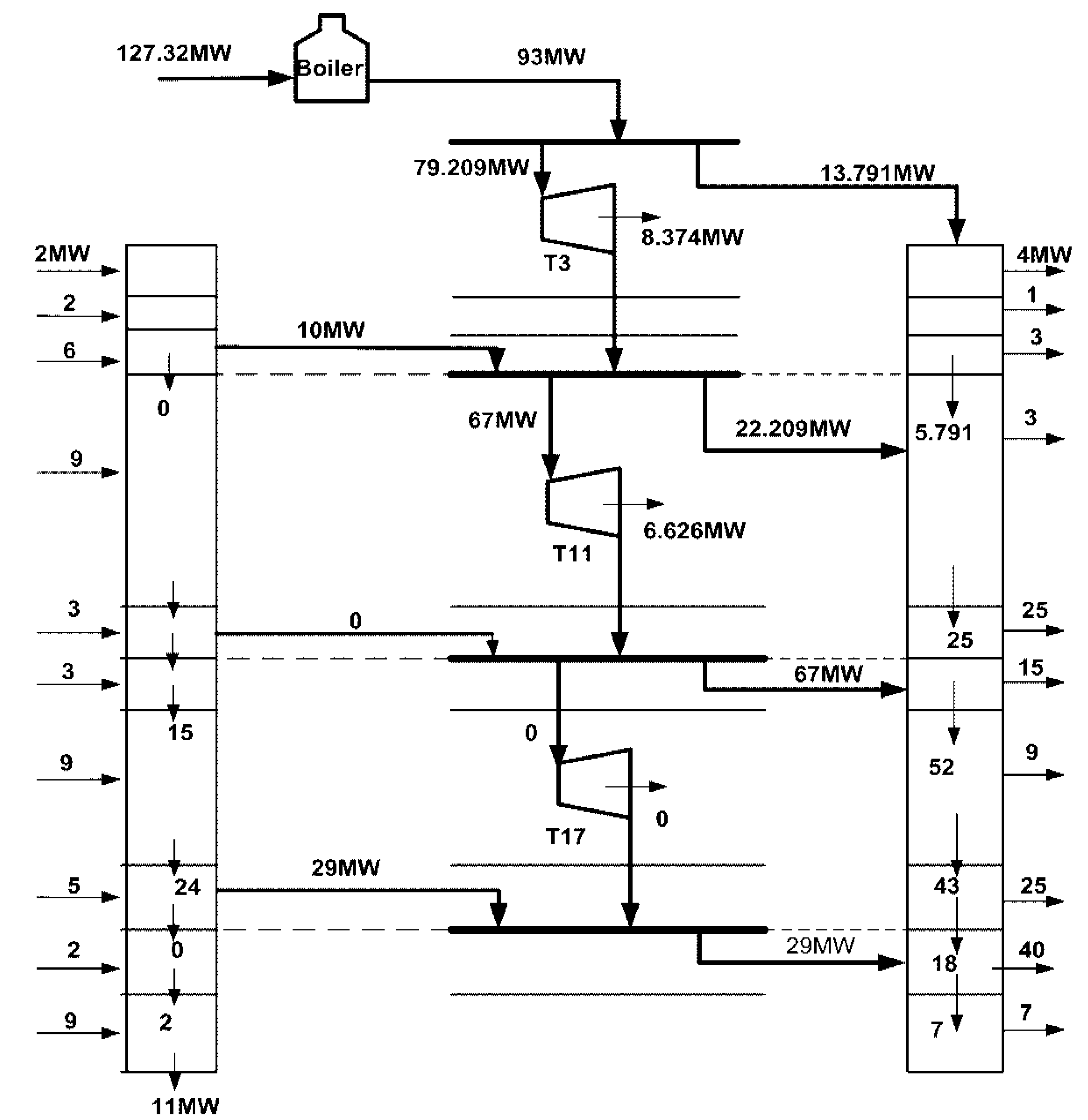
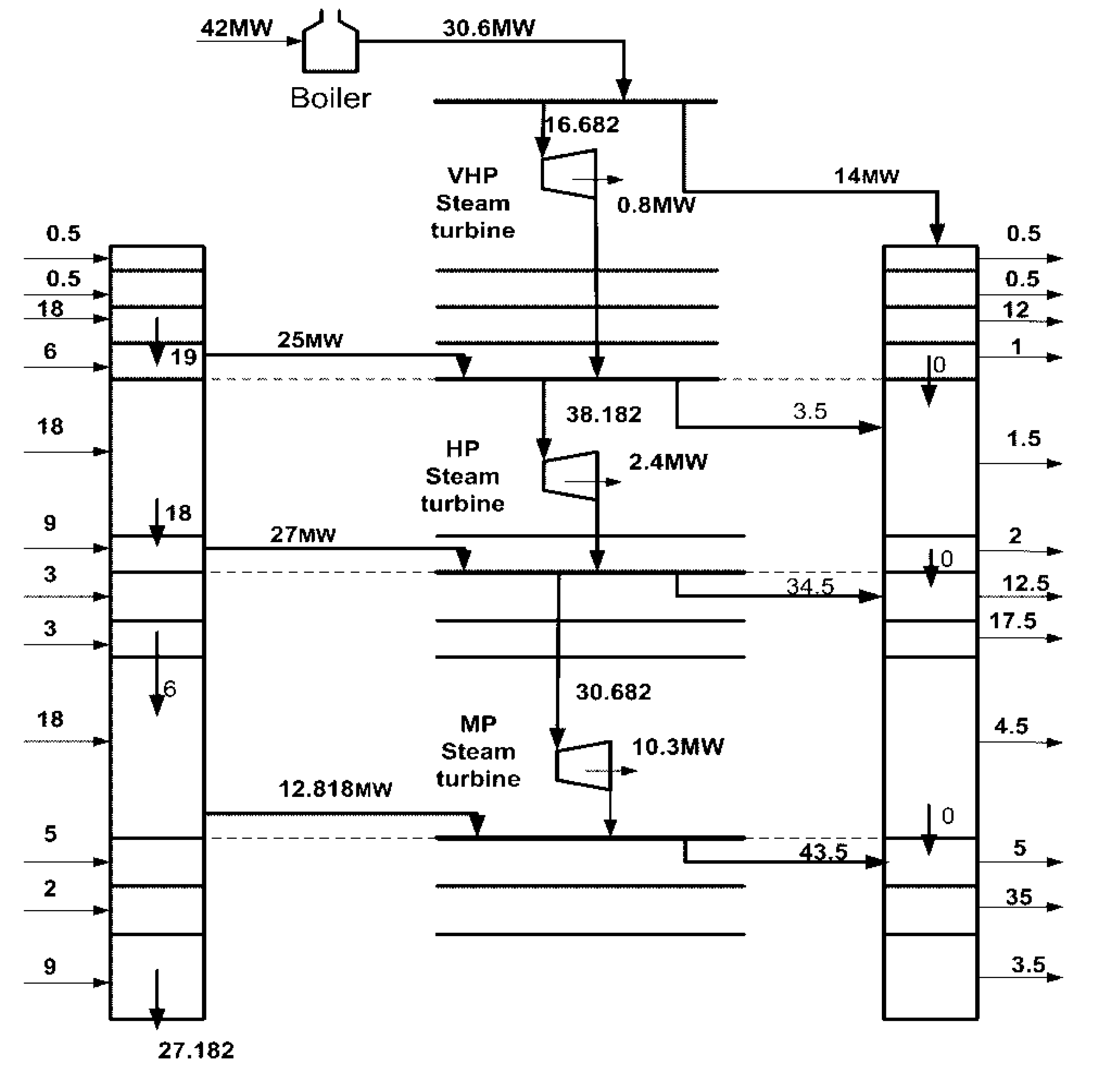
4.2. Case Study 2
| Heat Provided (MW) | Heat Required (MW) | Interval (i,j) | Pressure Steam Level (kPa) |
|---|---|---|---|
| 0.5 | 0.5 | (1,1) | 6411.7 |
| 0.5 | 12 | (1,2) | 5498.7 |
| 18 | 1 | (1,3) | 4688.6 |
| 6 | 1.5 | (1,4) | 3973 |
| 18 | 2 | (2,1) | 2317.8 |
| 9 | 12.5 | (2,2) | 1906.3 |
| 3 | 17.5 | (2,3) | 1553.8 |
| 3 | 4.5 | (2,4) | 1254.4 |
| 18 | 5 | (3,1) | 270.1 |
| 5 | 35 | (3,2) | 198.5 |
| 2 | 3.5 | (3,3) | 143.3 |


5. Conclusions
Nomenclature:
Cost rate, Cost rate associated with exergy [$/h] | |
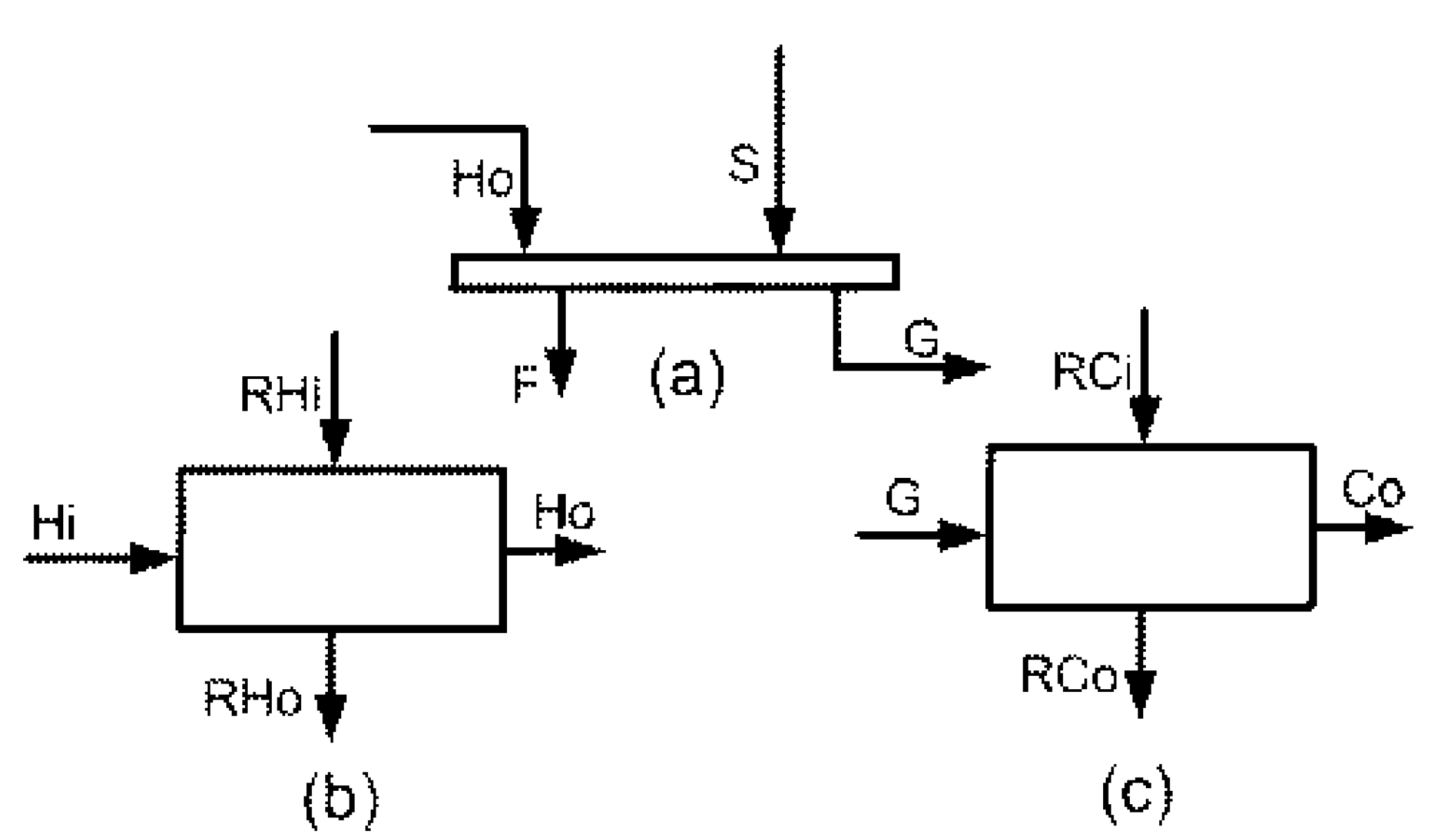
| Co | Heat flowing out of the temperature interval control volume to heat sink zone |
| c | Cost per unit of exergy [$/GJ] |
Exergy flow rate [kW] | |
| F | Heat flowing out of the steam level control volume to the steam turbine |
| G | Heat flowing out of the steam level control volume to the heat sink |
| Hi | Heat provided by process heat source to temperature interval control volume in heat source zone |
| Ho | Heat flowing out of the temperature interval control volume in heat source zone |
| HP | High Pressure |
| LP | Low Pressure |
| MP | Medium Pressure |
| RCi | Heat flowing into temperature interval control volume from a higher temperature interval into heat sink zone |
| RCo | Residual heat flowing out of temperature interval control volume in heat sink zone |
| RHi | Heat flowing into temperature interval control volume from a higher temperature interval into heat source zone |
| RHo | Residual heat flowing out of temperature interval control volume in heat source zone |
| S | Heat flowing into the steam level control volume from steam turbine |
| VHP | Very High Pressure |
Subscripts
| B | Boiler |
| D | Destruction |
| e | Exit |
| F | Fuel |
| i | Inlet |
| is | Isentropic |
| max | Maximum, refers to capacity |
| P | Product |
| q | Heat loss |
| sat | Saturation |
| sys | System |
| T | Turbine |
| w | Power |
References
- Nishio, M. Computer aided synthesis of steam and power plants for chemical complexes. Ph.D. Thesis, The University of Western, Ontario, Canada, 1977. [Google Scholar]
- Nishio, M.; Itoh, J.; Umeda, T. A thermodynamic approach to steam-power system design. Ind. Eng. Chem. Proc. Des. Dev. 1980, 19, 306–318. [Google Scholar] [CrossRef]
- Petroulas, T.; Reklaitis, G.V. Computer-aided synthesis and design of plant utility systems. AICHE J. 1980, 30, 69–78. [Google Scholar] [CrossRef]
- Papoulias, S.A.; Grossmann, I.E. A structural optimisation approach in process synthesis-I. Utility systems. Comput. Chem. Eng. 1983, 7, 695–706. [Google Scholar] [CrossRef]
- Mavromatis, S.P. Conceptual design and operational of industrial steam turbine networks. Ph.D. Thesis, The University of Manchester, Manchester, UK, 1996. [Google Scholar]
- Mavromatis, S.P.; Kokossis, A.C. Conceptual optimisation of utility networks for operational variations-1: targets and level optimisation. Chem. Eng. Sci. 1998, 53, 1585–1608. [Google Scholar] [CrossRef]
- Shang, Z. Analysis and optimisation of total site utility systems. Ph.D. Thesis, The University of Manchester, Manchester, UK, 2000. [Google Scholar]
- Shang, Z.; Kokossis, A. A transshipment model for the optimisation of steam levels of total site utility system for multiperiod operation. Comput. Chem. Eng. 2004, 28, 1673–1688. [Google Scholar] [CrossRef]
- Varbanov, P.S.; Doyle, S.; Smith, R. Modelling and optimization of utility systems. Chem. Eng. Res. Des. 2004, 82, 561–578. [Google Scholar] [CrossRef]
- Keenan, J.H. A steam chart for second low analysis. Mech. Eng. 1932, 54, 195–204. [Google Scholar]
- Lazzaretto, A.; Tsatsaronis, G. SPECO: A systematic and general methodology for calculating efficiencies and costs in thermal systems. Energy 2006, 31, 1257–1289. [Google Scholar] [CrossRef]
- Sahoo, P.K. Exergoeconomic analysis and optimization of a cogeneration system using evolutionary programming. Appl. Therm. Eng. 2008, 28, 1580–1588. [Google Scholar] [CrossRef]
- Abusoglu, A.; Kanoglu, M. Exergetic and thermoeconomic analyses of diesel engine powered cogeneration: Part 1—Formulations. Appl. Therm. Eng. 2009, 29, 234–241. [Google Scholar] [CrossRef]
- Abusoglu, A.; Kanoglu, M. Exergetic and thermoeconomic analyses of diesel engine powered cogeneration: Part 2—Application. Appl. Therm. Eng. 2009, 29, 242–249. [Google Scholar] [CrossRef]
- Tsatsaronis, G. Definitions and nomenclature in exergy analysis and exergoeconomics. Energy 2007, 32, 249–253. [Google Scholar] [CrossRef]
- Abusogolu, A.; Kanoglu, M. Exergoeconomic analysis and optimization of combined heat and power production: A review. Renew. Sust. Energy Rev. 2009, 13, 2295–2308. [Google Scholar] [CrossRef]
- Equip Cost: Boiler Cost. Available online: http://www.matche.com/EquipCost/Boiler.htm (accessed on 1 July 2011).
- Loh, H.P.; Jennifer, L.; Charles, W.W. Process Equipment Cost Estimation. Final Report for National Energy Technology Center. Available online: http://www.chemeng.lth.se/ket050/Arkiv/KostnadsDataProcessutrustning2002.pdf (accessed on 9 March 2012).
- Marshall & Swift Equipment Cost Index. Available online: http://business.highbeam.com/408261/article-1G1-254419142/marshall-amp-swift-equipment-cost-indexFigure.1 (accessed on 1 July 2011).
© 2012 by the authors; licensee MDPI, Basel, Switzerland. This article is an open access article distributed under the terms and conditions of the Creative Commons Attribution license (http://creativecommons.org/licenses/by/3.0/).
Share and Cite
Shamsi, S.; Omidkhah, M.R. Optimization of Steam Pressure Levels in a Total Site Using a Thermoeconomic Method. Energies 2012, 5, 702-717. https://doi.org/10.3390/en5030702
Shamsi S, Omidkhah MR. Optimization of Steam Pressure Levels in a Total Site Using a Thermoeconomic Method. Energies. 2012; 5(3):702-717. https://doi.org/10.3390/en5030702
Chicago/Turabian StyleShamsi, Shahin, and Mohammad R. Omidkhah. 2012. "Optimization of Steam Pressure Levels in a Total Site Using a Thermoeconomic Method" Energies 5, no. 3: 702-717. https://doi.org/10.3390/en5030702