Article

Calculation of the Arc Velocity Along the Polluted Surface of Short Glass Plates Considering the Air Effect

State Key Laboratory of Power Transmission Equipment & System Security and New Technology, Chongqing University, Chongqing 400044, China
*
Author to whom correspondence should be addressed.
Energies 2012, 5(3), 815-834; https://doi.org/10.3390/en5030815
Submission received: 22 February 2012 / Revised: 19 March 2012 / Accepted: 19 March 2012 / Published: 22 March 2012

Abstract

:
To investigate the microphysics mechanism and the factors that influence arc development along a polluted surface, the arc was considered as a plasma fluid. Based on the image method and the collision ionization theory, the electric field of the arc needed to maintain movement with different degrees of pollution was calculated. According to the force of the charged particle in an arc plasma stressed under an electric field, a calculation model of arc velocity, which is dependent on the electric field of the arc head that incorporated the effects of airflow around the electrode and air resistance is presented. An experiment was carried out to measure the arc velocity, which was then compared with the calculated value. The results of the experiment indicated that the lighter the pollution is, the larger the electric field of the arc head and arc velocity is; when the pollution is heavy, the effect of thermal buoyancy that hinders arc movement increases, which greatly reduces the arc velocity.

Graphical Abstract

1. Introduction

The discharge along the polluted surface of insulators is a major problem in power transmission systems, and it remains a hot issue in the field of high voltage insulation [1]. The formation and propagation of partial arcs along a polluted insulator surface has been the subject of many experimental and theoretical studies. In addition, many models have been presented to describe the discharge mechanisms [2,3,4,5]. Although many different models [6,7] covering each phase of the discharge process have been presented, these studies are mainly qualitative or experiential, and no related report on the microphysics mechanism has been detailed up to now. The force factors on the developing arc and the velocity characteristic of arc with the polluted degree along the polluted surface can provide theoretical support for a comprehensive understanding of the mechanism of polluted flashover.
An arc is a high-density charged particle flux and arc motion results from the collective motion of charged particles in an electric field. Therefore, arc motion can be described using fluid mechanics [8]. When the applied voltage meets the requirement of the flashover conditions, the arc is drawn by the electric field force towards the opposite electrode and a flashover is formed [9]. With the arc velocity changing constantly during arc development, different researchers have come up with different measurement results. Although various methods have been used to investigate the instantaneous arc velocity along the surface of polluted insulators [10,11], these are purely theoretical or purely empirical, and they are only valid under certain conditions. Theoretical research on surface discharge, which is mainly based on gas ionization discharge [12], did not consider the influence of insulator surface on the discharge. Although the body force was measured in the experiment [13], and the arc velocity was investigated using an electrolyte instead of a wet polluted layer [14], the conditions are still very different from those of the wet polluted layer of an actual insulator, therefore, reflecting the actual condition effectively is difficult.
In this paper, the electric field needed to keep arc moving ahead with different pollution degrees is given based on the image method and the collision ionization theory. Based on the force of the charged particles in the arc plasma stressed under the electric field, a calculation model of arc velocity, which is dependent on the electric field of the arc head, is presented; the effects of airflow around the electrode and air resistance were considered. The charge simulation method was employed to calculate the variation between the electric field of the arc head and the arc length with different degrees of pollution. The electric field was incorporated into the calculation model to obtain the arc velocity. An experiment was carried out to measure the arc velocity, and we compared the result with the calculated value. The results provide theoretical support for a comprehensive micromechanism of polluted flashover.

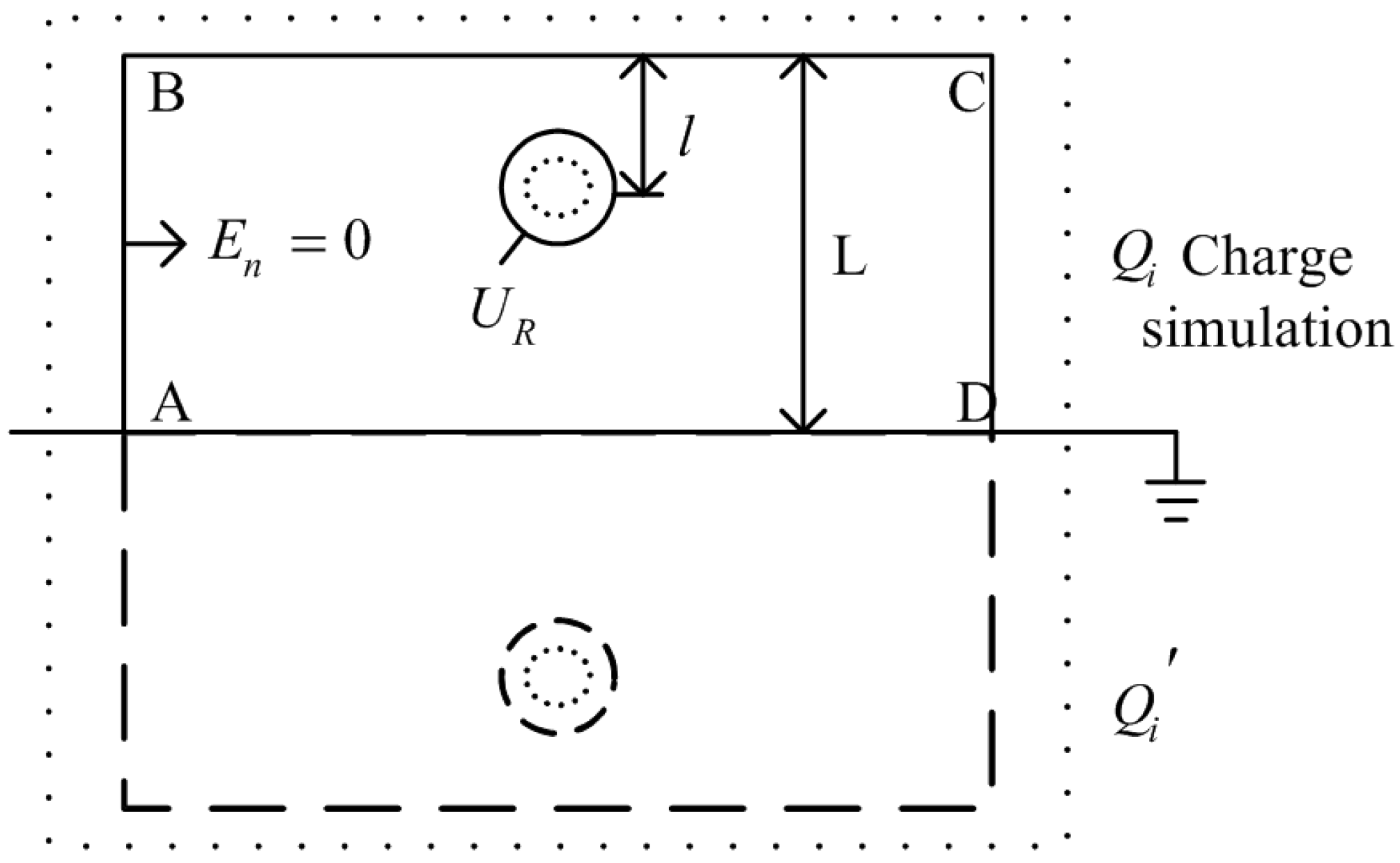
2. Electric Field for Maintaining Arc Movement

Supposing the arc head is a semisphere with radius r, the equivalent charge at the center of sphere is q, and the image charge in insulation medium is q/. The angle from the arc head to the center of sphere, that from the arc head to the image charge point is θ, and the distance from the arc head to the image charge point is r/. The dielectric constant of air is ε0, and the dielectric constant of insulation medium is ε1. Here, the insulation medium is toughened glass whose relative dielectric constant is 7.5, so ε1 = 7.5ε0. The image charge can be obtained by the following equation [15]:
q = ε 0 ε 1 ε 0 + ε 1 q = 0.7647 q
The negative sign indicates that the image charge has a charge opposite that of the initial charge. Supposing the electric property of q is positive, the direction of the electric field E 0 at the arc head is positive, and the electric field produced by q’ is E 1 . Therefore, the total electric field at the arc head is E s = E 0 + E 1 , as shown in Figure 1.
Figure 1. Schematic diagram of electric field at arc head.
Energies 05 00815 g001
Hence, the electric field is computed as follows:
E 0 = q 4 π ε 0 r 2
E 1 = | q | 4 π ε 0 r 2 = 0.1529 E 0
E s = E 0 2 + E 1 2 + 2 E 0 E 1 sin θ = 1.14 E 0
When the sum of the electric energy after the electron passes the main free path, the electron kinetic energy and ray radiation energy exceed the main ionization energy of the mixed gases at the arc head, the arc moves and fulfills the equation as follows:
E s e λ ¯ e + 3 2 k T e + h c / λ = U i e
where Es is the total electric field at the arc head considering the effect of the image charge, λ e ¯ is the mean free path of electron, k is the Boltzmann constant, Te is the electron temperature [16], Ui is the mean ionization potential of the mixed gases at the arc head, λ is the wavelength of arc light, and c is the velocity of light, h is Planck constant.
Based on the gas molecule phoronomy, the mean free path of gas molecule with diameter d at pressure p and temperature T is [17]:
λ g ¯ = k T 2 π d 2 p
Ignoring the electron radius, the electron velocity is much faster than gas molecule velocity, and the gas molecule can be considered as still. Therefore, the mean free path of the electron is 4 2 times of gas molecule with the same temperature [18], the mean free path of the electron with temperature Te is as follows:
λ e ¯ = 4 k T e π d 2 p
The effective molecule diameter of air is 0.35 nm [19], and the vapor molecule diameter is about 0.27 nm to 0.32 nm [20]. The mean value of 0.295 nm is the effective molecule diameter of vapor. The arc light is similar to sunlight [21], and the mean wavelength is λ = 0.475 μm.
NaCl is used to represent the soluble salt, and the equivalent salt deposit density (ESDD) is used to represent the degree of pollution. Suppose the ESDD is s mg/cm2 and the water adsorption capacity of salt dissolved completely per square centimeter is m mg, the saturation of NaCl at room temperature is 36 g/mL [22], so:
36 100 = s m
The adsorption capacity of water when the salt dissolves completely per square centimeter is:
m = 25 s 9
and the number of water molecules is:
n H 2 O = 25 s 9 × 10 3 × 6.02 × 10 23 18
At atmospheric pressure and room temperature, the number of air molecules per cubic centimeter is:
n 0 = 6.02 × 10 23 24041 = 2.504 × 10 19
Therefore, the proportion of the number of vapor and air molecules per unit volume at the arc head is:
n H 2 O n a i r = n H 2 O n 0 n H 2 O
According to the gas ionization potential [23] with the scaled value of each gas ionization potential as the mean ionization potential, then:
U i = 12.7 n H 2 O + 16.3 n a i r n H 2 O + n a i r
Similarly, the mean effective molecule diameter of the mixed gas at the arc head is:
d = 0.295 n H 2 O + 0.35 n a i r n H 2 O + n a i r
By replacing the Equations (2), (3), (4) and (7) into (5), the electric field at the arc head that is produced by the equivalent charge q is:
E 0 = U i e 3 2 k T e h c / λ 4.5552 e k T e × π d 2 p
The electric field required to maintain the arc movement along the insulation surface at the horizontal direction is:
E = E 0 0.1529 E 0 cos θ
The relationships between the horizontal electric field at the arc head and the proportion of mixed gas molecule number to the ESDD are shown in Figure 2. Curves E0 and E are the relationship between the electric field at the arc head in the horizontal direction and the ESDD with and without the image charge effect, respectively. Curve nwater/nair is the relationship between the ratio of the number of vapor to air molecules at the arc head and the ESDD. Figure 2 shows that the proportion of mixed gas molecules to the vapor molecules increases parabolically with the ESDD, and that the electric field required to maintain arc movement is inversely proportional to ESDD. Considering that the higher the ESDD, the higher the adsorption capacity of water to dissolve the salt completely and the mean ionization potential of mixed gas at the arc head, the electric field required to maintain arc development decreases with increasing ESDD. The higher the ESDD, the easier the arc moves forward. When the electric field at the arc head exceeds this electric field condition, the arc continuously moves forward until the flashover.
Figure 2. Relationships of the electric field at arc head in the horizontal direction with/without image charge effect (E/E0) and the proportion of mixed gas molecule number nwater/nair with the ESDD.
Energies 05 00815 g002

3. Arc Force Analysis and Velocity Calculation

3.1. Force Analysis of the Arc

Several physical mechanisms of discharge along the polluted surface have been proposed. One of the most widely accepted mechanisms is that external forces simply pull the partial arc across the surface [24]. With the in-depth study of plasma [25,26], a better understanding of its basic properties (components, thermodynamics, the transport and the electrical properties), basic physical processes (arc foot motion, the interaction between arc and airflow, electrode processes), and the flow, and heat transmission has been gained. Therefore, the electric field force and thermal buoyancy should be considered during the development of arc plasma, as well as the effects of the interaction between arc and airflow. As the high temperature arc plasma moves fast, the effect of electrode jet and air viscous action varies. Considering the factors that affect arc development synthetically, for a horizontal insulation flat plate, the arc is influenced mainly by the pressure of the airflow vortex [27] and the viscous resistance of the ambient air [28], aside from the resultant force of the electric field force [24]. These components work together to determine the arc motion characteristics. In the present study, the negative polar arc was taken as an example, with the arc moving tightly along the surface of insulation plate. If the direction of thermal buoyancy is perpendicular to the horizontal plane, the effect of thermal buoyancy can be ignored. The force analysis is shown in Figure 3.
Figure 3. Schematic diagram of force analysis of arc.
Energies 05 00815 g003
The forces of the arc stress during the prolongation along the polluted surface are expressed as follows:
F = F E + F P + f
where FE is the electric force of arc, FP is the airflow pressure force, f is the air resistance.

3.1.1. The Forward Electric Field Force

The electric force FE is in the order ε0E2/2 times the characteristic area given by [24]:
F E = 1 2 ε 0 E 2 r 2
where ε0, E, and r are the permittivity of free space, the head field of arc, and the arc radius, respectively.

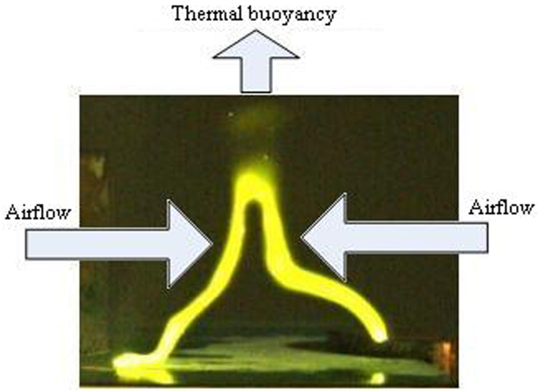
3.1.2. The Forward Airflow Pressure Force

During arc movement, an airflow vortex occurs at the back of the arc, as shown in Figure 3. Supposing the arc constriction radius at point a of the electrode vicinity is ra = a, and the radius at point b of the arc head is rb = b, (a << b). Thus, the axial pressure difference [27] ΔP and the airflow pressure force FP between points a and b are given by:
Δ p = μ 0 I 2 4 π 2 ( 1 r a 2 1 r b 2 ) μ 0 I 2 4 π 2 a 2
F P = Δ P S μ 0 I 2 4 π
where I is the arc current, and μ0 is the permeability of free space 4π × 107 H/m.

3.1.3. Backward Air Resistance

The velocity is very slow at the beginning of the arc, and it suffers mainly from the viscous resistance in prolongation. Assume that the arc is a size of a column; the air resistance f equals to the viscous resistance [28] f1 of air around the arc can be written as:
f 1 = η π r ( r + 2 l ) d v d x
where η is the coefficient of air viscosity, l is the length, and dv/dx is the variation in arc velocity per unit displacement.
The force that drives the arc to move forward is the sum of the electric field force and airflow pressure. Based on Newton’s law, acceleration can be expressed as:
d v d x = F E + F P m 1
where m1 is the mass per unit area of the air ahead of the arc.
By substituting (18), (20), and (22) into (21), and letting g = l/r, we obtain:
f 1 = η ( 1 + 2 g ) ρ 0 ( F E + F p )
where ρ0 is the air density of 1.293 kg/m3.
If the arc is moving forward to the grounding electrode, the resultant force ΔF on the arc in the horizontal direction can be expressed as:
Δ F = F P + F E f 1 = ρ 0 η ( 1 + 2 g ) ρ 0 ( F E + F p )
The motion conditions of partial arc in the horizontal direction are obtained as follows:
(1)
When the resultant force is larger than the air resistance ΔF > 0, then g < (ρ0/η – 1)/2, and the arc moves forward.
(2)
When the resultant force is equal to or smaller than the air resistance ΔF ≤ 0, then g ≥ (ρ0/η – 1)/2, the arc is extinguished or remains static.

3.2. Arc Velocity Calculation

3.2.1. Velocity Caused by the Electric Field Force

If the arc velocity is v1 when the length is l under the field force, based on the theorem of kinetic energy, the equation can be expressed as:
F E l = 1 2 m 2 v 1 2 0
where m2 is the mass of the arc, and m2 = ρπr2l.
By substituting the electric field force FE and the mass differential expression of arc m2 into Equation (25), we will have:
0 l 1 2 ε 0 E 2 r 2 x d x = 1 2 0 l 2 3 π r 3 ρ d x v 1 2
where ρ is the arc density in air, and ρ = ρ0/30.
According to (26), we obtain:
v 1 = E 2 3 ε 0 g π ρ

3.2.2. Velocity Caused by Airflow Pressure

Considering the pressure at the arc axes is much less than the total pressure, the pressure gradient at the axes drives the arc to move forward. If the velocity of the arc caused by airflow pressure is v2, the electrode jet is stopped and a kinetic preventive pressure ρv22/2 is produced. The electrode jet velocity can be calculated using the pressure difference given in Equation (18), which is equal to the kinetics preventing pressure, as given by [27]:
Δ P p a = ρ v 2 2 2
By substituting Equation (19) into (28), we obtain:
v 2 = I π a μ 0 2 ρ
According to [6], the current can be expressed by the relation:
I = k E 2 l
We can then obtain:
v 2 = k E 2 l π a μ 0 2 ρ
where k is a constant.
Hence, the velocity v0, which drives the arc to move forward, is the sum of v1 and v2:
v = v 1 + v 2 = k E 2 l a π μ 0 2 ρ + E 2 3 ε 0 g π ρ

3.2.3. Velocity Caused by Air Resistance

The viscosity coefficient η around the arc changes with the air temperature. The variation meeting the Sutherland formula is given by [28]:
η η 1 = T 1 + T s T + T s ( T T 1 ) 3 2
where T1 is reference temperature, η1 is the air viscosity coefficient at the reference temperature, and Ts is the Sutherland constant, which is about 120 K.
The temperature is less than 5000 K at the beginning of arc formation, and the flashover reaches up to about 13,000 K [11]. In this paper, T = 4000 K, T1 = 273 K, η1 = 1.71 × 10⁻⁵ pa·s. We obtain:
η = 393 T + 120 ( T 273 ) 3 2 × 1.71 × 10 5
The arc temperature increases with the arc length based on the measured range of arc temperature [11] if the arc temperature can be expressed by the linear relation:
T = 4000 + l L × 9000
where L is the length of the plate insulator.
When the arc velocity increases, the number of molecules per unit volume of the pre-arc and post-arc parts are different, and it leads to pressure resistance f2 expressed as:
f 2 = η ρ 0 r l v 2
Therefore, the resistance that the fast arc suffers in air is the sum of f1 and f2. We obtain:
f = f 1 + f 2 = η ( π r 2 + 2 π r l ) d v d x + η ρ 0 r l v 2
Again, if the decrease in velocity caused by air resistance is Δv, the approximate power equation is represented by the following expression:
f v = m 2 ( v 3 ) 2 2
We obtain:
v 3 = v η ( r + l ) ( 2 Δ p π + ε 0 E 2 ) π r ρ 0 2 + 2 η l v 3 π r
The velocities can be added directly because they are in a line, so the velocities can be added directly. According to (32) and (39), the practical velocity of arc v is:
v = v 1 + v 2 v 3

3.3. Calculation Results

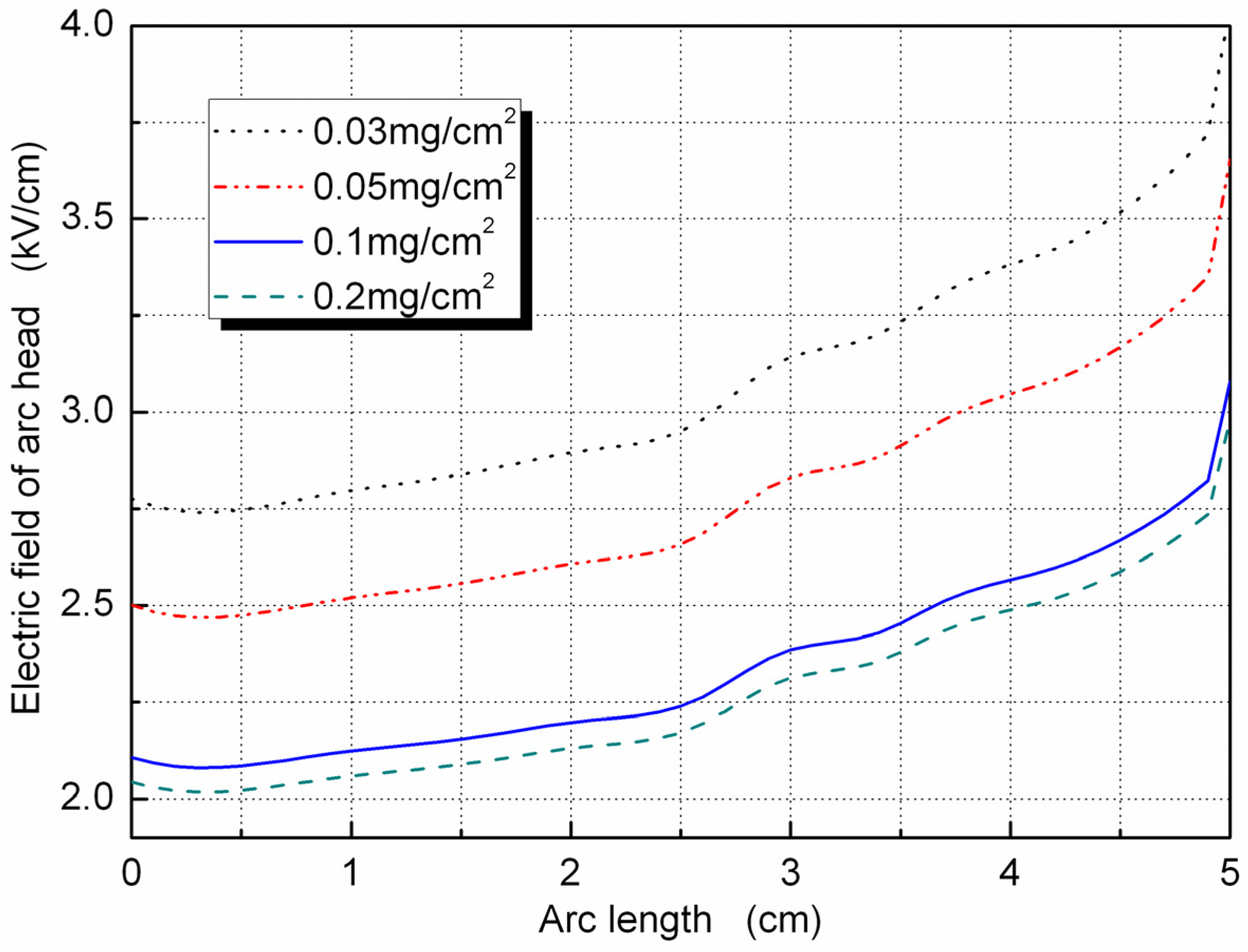
3.3.1. Electric Field of the Arc Head

Based on the investigation of force analysis on the arc and its effect on arc velocity, the arc velocity was found to be dependent on the electric field of the arc head. In this paper, the developing velocity of the arc along the horizontal polluted surface is investigated. The study only needs the electric field strength of the arc head in the horizontal direction.
The effect of air on the polluted surface layer and insulation medium can be ignored with the development of the arc. Moreover, the electric field distribution in the polluted layer depends on the current distribution on the insulation surface. The arc can be considered as a current source, and a constant current field consists of the polluted layer and the current source. The current flows from the arc and receives compensation from the system power supply at the same time. The electric charge in the arc keeps a dynamic balance; hence, it can be considered as an electrostatic field.
Based on the fundamental equations of constant current field in conducting medium:
{ J = 0 × E = 0 J = γ E 2 φ = 0
At the boundary face, those equations satisfy the conditions:
{ φ 1 = φ 2 γ 1 φ 1 n = γ 2 φ 2 n
where E and J are the electric field intensity and current density, respectively; φ is the electric potential, γ is the conductivity. φ1 and φ2 are the electrical potentials at each side of the interface, respectively; γ1 and γ2 are the conductivities at each side of the interface, respectively. n is the normal direction.
The generally accepted charge simulation method is employed to calculate the electric field of the arc head. The results were then used to calculate the arc velocity. For a rectangular flat plate, the constant current field in a polluted layer is similar to the two-dimensional space electric field. The two-dimensional electric field is a parallel plane field, and the axial length is infinite. The ground is treated as a zero potential energy surface, and the imaging method is employed to satisfy the grounding boundary condition of the polluted surface. The schematic diagram of the calculation is shown in Figure 4.
The shunting effect of the polluted layer on both sides of the arc is ignored. Suppose that only the arc root is in contact with the pollution layer, and that the arc moves ahead against the insulation surface. The empirical formula of the arc radius and current is given by [29]:
r = I 1.45 π
In this study, the boundary condition UR is the surface potential of the arc root, and the field normal component at the pollution layer boundary of AB, BC, and CD all equal to zero, viz. En = 0. A number of point charges inputted at the arc root and boundary to satisfy the following boundary condition:
{ U R = U A I n l U n | A B , B C , C D = 0
where U and I are voltage and current, respectively, A and n are the arc constants relating to the cooling conditions, ambient media, and so on, for the polluted flashover A = 63, n = 0.76 [30].
Figure 4. Schematic diagram of the charge simulation method.
Energies 05 00815 g004
The number of simulated charges selected from the concentric circle in the arc root is n1, and the same number of sites is taken at the arc root boundary. Meanwhile, the sum of the simulation charges taken at a certain distance outside of the boundary AB, BC, and CD is n2, and the same number of sites is taken at the boundary to satisfy the requirement that the field normal component equals to zero for each point. If n = n1 + n2, the equations of potential coefficients and field coefficients based on the uniqueness theorem of the electrostatic field are as follows:
U 1 = P 11 Q 1 + P 12 Q 2 + + P 1 n Q n U 2 = P 21 Q 1 + P 22 Q 2 + + P 2 n Q n U = P n 1 1 Q 1 + P n 1 2 Q 2 + + P n 1 n Q n
0 = B 11 Q 1 + B 12 Q 2 + + B 1 n Q n 0 = B 21 Q 1 + B 22 Q 2 + + B 2 n Q n 0 = B n 2 1 Q 1 + B n 2 2 Q 2 + + B n 2 n Q n
where B and P represent the potential coefficient and field coefficient matrix, respectively. U is the potential matrix.
By combining Equations (43) to (44), the simulation charge quantity and sites can be obtained. Moreover, the field of the arbitrary point of the arc root surface and boundary lines can be calculated using the simulation charge. The calculated results and the known conditions are then compared, which indicated an error. If the error is within the allowable range, the calculation method can be used to determine the field and the potential of the arbitrary point in a passive field. If the error exceeds the acceptable range, the number and position of the simulation charge must be reselected until the requirement is met.
The tangential field can be calculated at the arbitrary position on the plate surface, that is, the vector sum of the tangential field of all the simulation charges at a certain point. The tangential field can be written as:
E j = i = 1 n B j i Q i cos θ j i
where Ei is the tangential field at the arbitrary point, Bji is the field coefficient of simulation charge i at the point j, Qi is the quantity of simulation charge i, θji is the included angle between the field direction of the simulation charge i at the point j with the horizontal direction.
The conductance (γ) of the pollution layer and the critical flashover voltage (Uc) correspond with the ESDD of 0.03, 0.05, 0.1 and 0.2 mg/cm2 are given in Table 1 [31]. In this paper, the length and width of the rectangular plate are 5 and 20 cm, respectively. Each simulation charge is set along the boundary tangent at an interval of 0.39 cm outside the polluted layer boundary of 0.2 cm, and 36 simulation charges are set at half of the radius in the arc root. At the ground surface with zero potential energy as a plane of symmetry, and chose the same number of image charge to satisfy the requirement for the grounding condition. The field error of the checkpoint on the boundary is 0.054%, which satisfies the error requirement of less than 1%.
Table 1. Initial experimental data.
ESDD (mg/cm2)γ (μS·cm−1)Uc (kV)
0.033.610.44
0.055.59.17
0.1117.45
0.2205.57
By substituting the experimental data into Equations (44) and (47), the variations in the electric field of the arc head with the arc length can be obtained, as shown in Figure 5. Figure 5 shows that the electric field of the arc head increases with increasing arc length, and decreases with increasing degree of pollution. The arc head field at a low degree of pollution is larger than that at a high one during the whole process. It ranges from the beginning of the arc to the end of the flashover. The electric field at the ESDD of 0.03 mg/cm2 is three times larger than that of 0.2 mg/cm2 at the same length of arc. For the high conductivity of the arc, most of the voltage is concentrated on both sides of the residual polluted layer. The electric field of the arc head is enhanced with increasing arc length. With the same arc length, the larger the conductivity of the polluted layer is, the lower the voltage is distributed on it. Therefore, the arc head field becomes much smaller. Meanwhile, the larger the conductivity of the polluted layer is, the larger the leakage current is. The dry band is formed easily near the electrode with a concentrated field, and so can the partial arc.
Figure 5. Variation of the electric field of the arc head with the arc length.
Energies 05 00815 g005

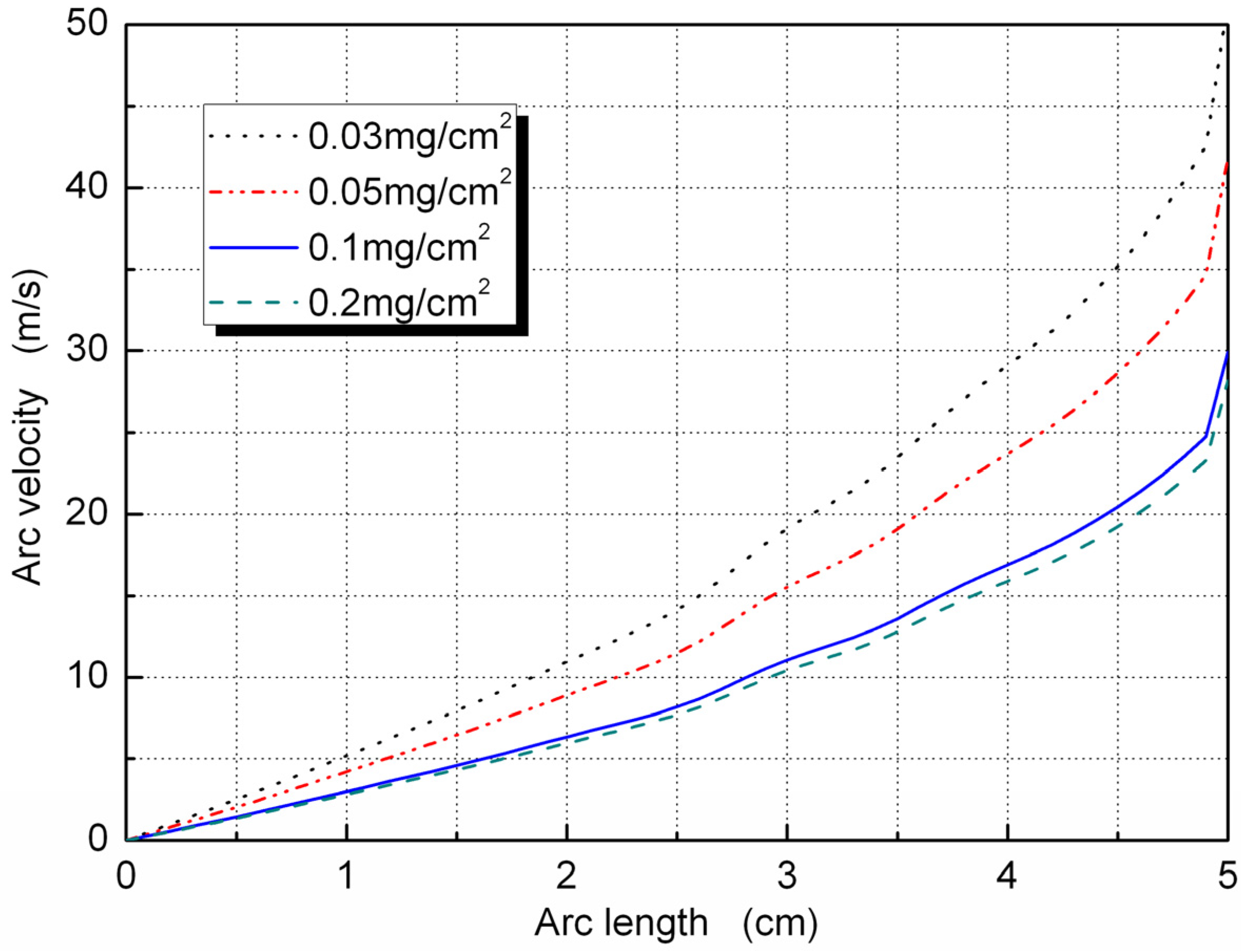
3.3.2. The Arc Velocity

By substituting the result of the electric field of the arc head into Equation (40), the variation of the calculated velocity with the arc length is shown in Figure 6. Clearly, the developing velocity increases with the increment of the arc length no matter how high the degree of pollution. However, the developing velocity is reduced with increasing degrees of pollution at the same arc length. At the beginning of the partial arc, the arc velocities of different pollution degrees have a few differences; all are less than ten meters per second. The biggest difference is the velocity of the critical flashover; when the pollution degree is 0.2 mg/cm2, the maximal speed is about less than 30 meters per second. The maximal speed reaches up to 50 m/s with the pollution degree of 0.03 mg/cm2.
Figure 6. Variation of the calculated velocity with the arc length.
Energies 05 00815 g006

4. Test Specimens, Setups and Procedures

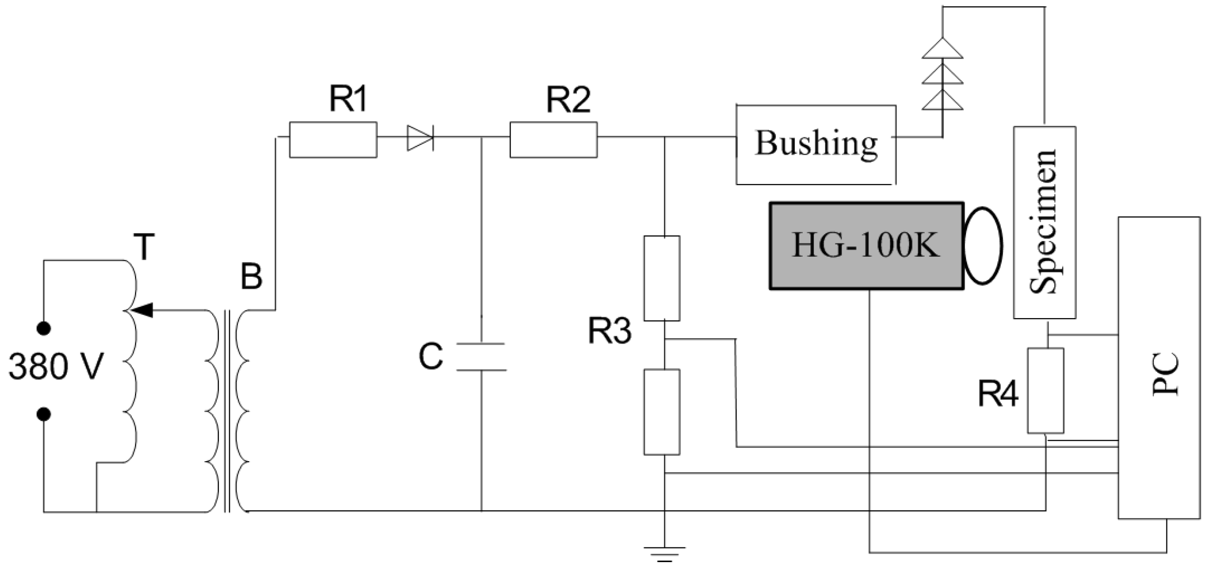
4.1. Test Specimens and Setups

To validate the calculation model based on the force analysis proposed in this paper, a pollution test of a flat insulator plate model measuring 20 cm × 20 cm × 1 cm was carried out. The circuit of the pollution test under DC voltage is shown in Figure 7. Through this system, the value of the applied voltage and the leakage current could be measured. The position of the arc could be measured synchronously as well.
Figure 7. Test circuit. T-regulator, B-transformer, R1/R2-protective resistance, C-filtering capacitance, R3-resistance divider, R4-standard resistance.
Energies 05 00815 g007
The test power supply consisted of a regulator and a transformer. The main parameters of the regulator were the rated capacity of 100 kVA, the input voltage of 380 V, and the output voltage range of 0 V to 400 V. The main parameters of the transformer were a rated capacity of 200 kVA, a rated current of 1 A, an input voltage range of 0 V to 400 V, and an output voltage range of 0 kV to 200 kV. The DC power supply was generated by a silicon stack to rectify the AC voltage. At a leakage current of 1 A, the dynamic voltage was less than 5%, and the ripple coefficient of the voltage was less than 3% at the flashover time, which satisfies the requirement recommended by the IEC Tech. Rep. GB/T 22707 [32] and IEEE Standard-4-1995 [33]. The test power supply was introduced into the artificial pollution laboratory using a wall bushing. The high test voltage side was connected with the data acquisition system through a DC resistance divider with a voltage ratio of 1:10000. The data acquisition system was used to collect the data of the applied voltage and leakage current synchronously using an NI USB-6215 data acquisition card. The data acquisition card collects samples at a non-inductive resistance of 1 Ω between the grounding electrode and the ground. To avoid the over-current during the test, the protective resistances of R1 with 5 kΩ and the R2 with a bushing filled with distilled water conductance less than 5 μS·cm−1, were used.

4.2. Test Procedures

Before the test, all specimens were carefully cleaned so that all traces of dirt and grease on the glass insulation surface were removed. The solid layer method was applied to the polluted layer on the specimens where sodium chloride and kaolin were the electric and inert materials, respectively [34]. Considering the common proportion of sodium chloride and kaolin in engineering is 1:6, four specimens with ESDD of 0.03, 0.05, 0.1, and 0.2 mg/cm2 were prepared. To achieve precision and uniformity of pollution distribution on the insulation surface, the weight of the sodium chloride and kaolin was first calculated based on the area of the glass plate for every pollution grade. The sodium chloride and kaolin were weighed using a digital balance with a precision of 0.1 mg, and were placed on the glass insulation surface. Distilled water was dropped until the sodium chloride and kaolin dissolved completely. A filament was glided back and forth along the glass surface until a uniform pollution solution film was formed. Three groups of specimens for each pollution grade were prepared, and were then placed at a shady and cool place to dry naturally. Before the test, distilled water was sprinkled onto the polluted layer uniformly on the glass plate until the polluted layer dissolved completely. The DC voltage was then applied to the specimens and was increased with a constant rate of 1 kV/s until the flashover. Each group of specimen was tested ten times, and a five minute intervals was taken between the two adjacent tests. The high-voltage electrode used was a copper column with a height and diameter of 5 cm. The grounding electrode was a sheet copper with the same diameter.
The HG-100K high-speed camera was used to record the position and time by taking photos during the arc discharges. Based on the relationship between the development of partial arc and the corresponding time, the arc instantaneous velocity at time t2 can be expressed as:
v ( t 2 ) = l ( t 2 ) l ( t 1 ) t 2 t 1
where v(t2) is the instantaneous arc velocity, and l(ti) is the length of the arc at time ti (i = 1 or 2). If the interval between t1 and t2 is short enough, v(t2) can be treated as the instantaneous velocity at l(t2).

5. Analysis and Discussion
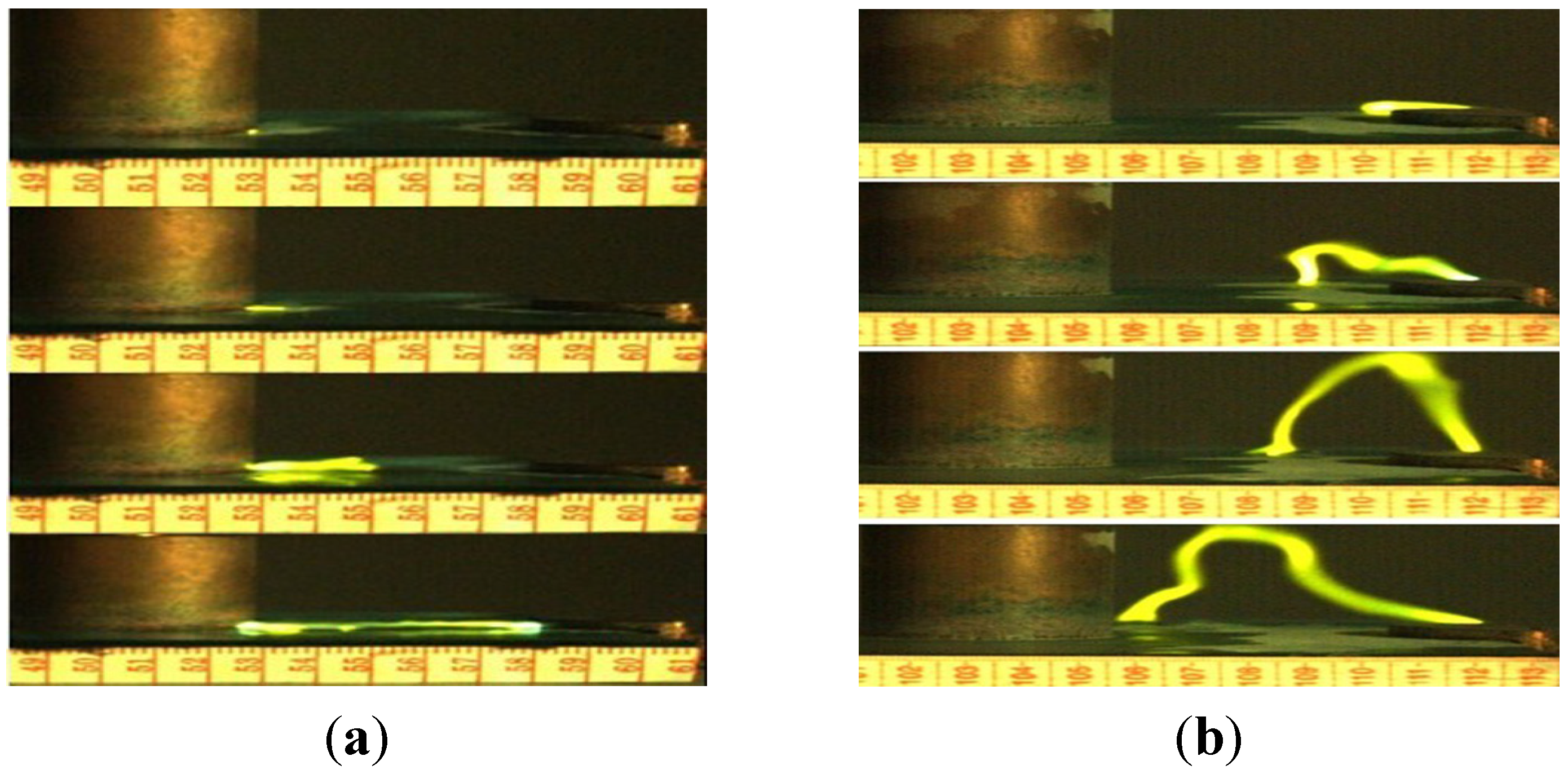
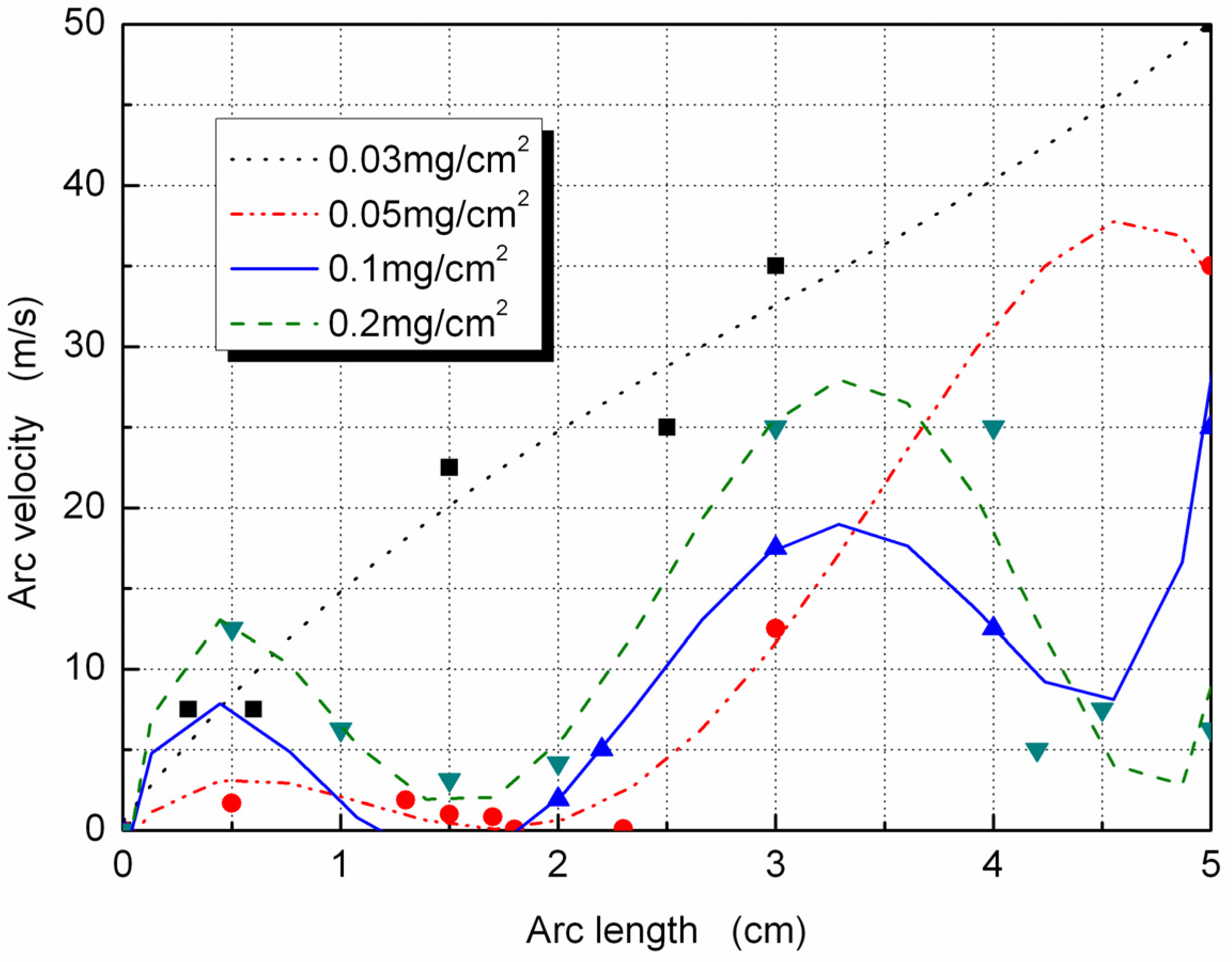
A short polluted glass plate with an anode–cathode distance of 5 cm was used to validate the proposed model. A column electrode and a semicircle grounding electrode with a radius of 2.5 cm were employed. Figures 8(a) and 8(b) are typical photos of development arc along the polluted surface with ESDD of 0.05 and 0.2 mg/cm2, respectively.
Figure 8. (a) Typical photos of development arc along the polluted surface with ESDD of 0.05 mg/cm2; (b) Typical photos of development arc along the polluted surface with ESDD of 0.2 mg/cm2.
Energies 05 00815 g008
As shown in Figure 8, the arc moves tightly along the surface of the insulation plate at low ESDD, the effect of thermal buoyancy is obvious with a high ESDD. We can determine arc position and the corresponding intervals from the photos at any time, and use Equation (48) to calculate arc velocity at any position. Similarly, we can determine the arc velocity with degrees of pollution of 0.03, 0.05, 0.1, and 0.2 mg/cm2.

5.1. Arc Velocity

The variations of the measured velocity with the arc length are shown in Figure 9. Figure 9 shows that the maximal velocity of the arc is only about tens of meters per second, not hundreds or thousands of meters per second [10]. The experiment indicates that there is no obvious difference in arc velocity at the same ESDD for which electrode the arc was formed, high voltage electrode or grounding one, and the arc velocity has a fluctuation with the development of arc. Except at a low ESDD of 0.03 mg/cm2, all arc velocities increased fast and then slowed down, and increased with fluctuations. With increasing arc length, the velocity increases again up to tens of meters per second at flashover time, which is consistent with the value calculated from the proposed model. The measured value is slightly different with the calculated value because the transition region at the arc head is not obvious. Consequently, an error in reading the arc length and the effect of thermal buoyancy occurs in the theoretical calculation.
Figure 9. Variation of the measured velocity with the arc length.
Energies 05 00815 g009
At a high ESDD, the difference between the calculated value and the measured value was large because more water was adsorbed to dissolve the salt completely. The more the salt and the water, the more charged particles were present in the arc; hence, the effect of thermal buoyancy is obvious, as shown in Figure 10. Such effect is brought by the airflow hindering the arc from moving toward the arc head. Moreover, the current flows easily in the conducting film when the polluted layer resistivity is high, and the streamer weakens to form at the arc head. When the arc length is long, the large thermal buoyancy leads to a steady arc, which slows down the arc velocity before flashover.
Figure 10. Schematic diagram of airflow caused by thermal buoyancy.
Energies 05 00815 g010

5.2. The Temperature Effect on the Arc Velocity

By comparing Figure 6 and Figure 9, the largest difference between the measured and the calculated value of arc velocity shows that the arc velocity displays an obvious fluctuation. The fluctuation occurs because the temperature of the arc plasma increases rapidly with the development of the arc, which changes the isobaric heat capacity of air around the arc and the heat exchange between them. Those changes may lead to the fluctuation of arc velocity in the discharge process.
The air isobaric heat capacity changes greatly with the temperature, and so does the arc plasma [35]. The isobaric heat capacity is stable and small at a temperature of 5000 K, which corresponds to the initial stage of arc development. Additionally, the leakage current, arc radius, and velocity are all small. With increasing temperature, the arc isobaric heat capacity, current, and velocity all increased rapidly. The isobaric heat capacity reaches a maximal value at 7500 K, which corresponds to the second stage of arc development. However, the isobaric heat capacity decreases rapidly to the minimum level with increasing temperature close to 10,000 K. The rapid decrement of isobaric heat capacity suddenly increases the loss of heat exchange and slows down the arc velocity. For the continuous power supply, the temperature consistently increased. Once the temperature exceeded 10,000 K, the isobaric heat capacity of the arc increased rapidly again, whereas the isobaric heat capacity of the ambient air did not increase at the same time. Therefore, the heat that cannot dissipate in time drives the arc to move quickly to the opposite electrode, and the flashover is formed.

6. Conclusions

This work focused on the arc velocity along the polluted insulation surface with an anode–cathode distance of 5 cm. The analysis of the calculation and experimental results are as follows:
(1)
Based on the image method and the collision ionization theory, the electric field of the arc needed to keep moving with different degrees of pollution was calculated.
(2)
Considering the electric force stressed on the charged particle in the electric field and the effect of airflow and ambient air on the moving arc, the characteristics of arc velocity along the polluted insulation surface were investigated.
(3)
Based on force analysis, a mathematical expression was presented, which allows one to evaluate the propagation velocity of the arc along the polluted surface. Only the physical parameters, such as the degree of pollution, insulation plate length, and critical flashover voltage were offered.
(4)
The electric fields of the arc head and arc velocities with degrees of pollution of 0.03, 0.05, 0.1, and 0.2 mg/cm2 were calculated, and an experiment was carried out. At the ESDD of 0.03 mg/cm2, the proposed model was consistent with the experiment. When the ESDD exceeds 0.2 mg/cm2, the airflow caused by thermal buoyancy hindered the arc from moving towards the arc head because of the large current and arc radius, and the reduced arc velocity.
(5)
The velocity, which was not a fixed value, changed with the variations in the degree of pollution and the electrode gap. No matter what type of electrode from which the arc developed from, no obvious difference in arc velocity at the same degree of pollution and electrode gap.

Acknowledgments

This work is supported by the Funds for Innovative Research Groups of China (51021005) and the National Basic Research Program of China (973 Program) (2009CB724504).

References

  1. Subba Reddy, B.; Kumar, U. Enhancement of surface flashover performance of high voltage ceramic discinsulators. J. Mater. Eng. Perform 2011, 20, 24–30. [Google Scholar]
  2. Su, H.; Jia, Z.; Guan, Z.; Li, L. Mechanism of contaminant accumulation and flashover of insulator in heavily polluted coastal area. IEEE Trans. Dielectr. Electr. Insul. 2010, 17, 1635–1641. [Google Scholar] [CrossRef]
  3. El-A Slama, M.; Beroual, A.; Hadi, H. Analytical computation of discharge characteristic constants and critical parameters of flashover of polluted insulators. IEEE Trans. Electr. Insul. 2010, 17, 1764–1771. [Google Scholar]
  4. Jiang, X.; Yuan, J.; Shu, L.; Zhang, Z.; Hu, J.; Mao, F. Comparison of DC pollution flashover performances of various types of porcelain, glass, and composite insulators. IEEE Trans. Power Deliv. 2008, 23, 1183–1190. [Google Scholar] [CrossRef]
  5. Dhahbi-Megriche, N.; Beroual, A.; Krähenbühl, L. A new proposal model for flashover of polluted insulators. J. Phys. D: Appl. Phys. 1997, 30, 889–894. [Google Scholar] [CrossRef]
  6. Waters, R.T.; Haddad, A.; Griffiths, H.; Harid, N.; Sarkar, P. Partial-arc and spark models of the flashover of lightly polluted insulators. IEEE Trans. Dielectr. Electr. Insul. 2010, 17, 417–424. [Google Scholar] [CrossRef]
  7. Gençoglu, M.T.; Cebeci, M. The pollution flashover on high voltage insulators. Electr. Power Syst. Res. 2008, 78, 1914–1921. [Google Scholar] [CrossRef]
  8. Li, X.; Chen, D.; Wu, Y.; Dai, R. A comparison of the effects of different mixture plasma properties on arc motion. J. Phys. D: Appl. Phys. 2007, 40, 6982–6988. [Google Scholar] [CrossRef]
  9. Shrzan, K.L.; Moro, F. Concentrated discharges and dry bands on polluted outdoor insulators. IEEE Trans. Power Deliv. 2007, 22, 466–471. [Google Scholar] [CrossRef]
  10. Balmain, K.G.; Gossland, M.; Reeves, R.D.; Kuller, W.G. Optical measurement of the velocity of dielectric surface arcs. IEEE Trans. Nuclear Sci. 1982, 29, 1615–1617. [Google Scholar] [CrossRef]
  11. Li, S.; Zhang, R.; Tan, K. Measurement of dynamic potential distribution during the propagation of a local arc along a polluted surface. IEEE Trans. Electr. Insul. 1990, 25, 757–761. [Google Scholar] [CrossRef]
  12. Larigaldie, S. Mechanisms of spark propagation in ambient air at the surface of a charged dielectric. II. Theoretical modeling. J. Appl. Phys. 1987, 61, 102–108. [Google Scholar] [CrossRef]
  13. Kotsonis, M.; Ghaemi, S.; Veldhuis, L.; Scarano, F. Measurement of the body force field of plasma actuators. J. Phys. D: Appl. Phys. 2011, 44, 045204. [Google Scholar] [CrossRef]
  14. Boylett, F.D.A.; Maclean, I.G. The propagation of electric discharges across the surface of an electrolyte. Proc. R. Soc. Lond. A 1971, 324, 469–489. [Google Scholar] [CrossRef]
  15. Feng, C.; Ma, X. Introduction of Engineering Electromagnetic Field; Higher Education Press: Beijing, China, 2000; pp. 40–43. [Google Scholar]
  16. Rethfeld, B.; Wendelstorf, J.; Klein, T.; Simon, G. A self-consistent model for the cathode fall region of an electric arc. J. Phys. D: Appl. Phys. 1996, 29, 121–128. [Google Scholar] [CrossRef]
  17. Li, C.; Zhang, L.; Qian, S. Calorifics; Higher Education Press: Beijing, China, 1978; pp. 111–116. [Google Scholar]
  18. Yao, Z.; Zhen, X.; Feng, X. Physical Electronics; Xi’an Jiaotong University Press: Xi’an, China, 1991; pp. 145–146. [Google Scholar]
  19. Li, C.; Zhang, L.; Qian, S. Thermotics; Higher Education Press: Beijing, China, 1978; p. 114. [Google Scholar]
  20. Li, C.; Fu, B. Application Chemistry Manual; Chemical Industry Express: Beijing, China, 2007; pp. 102–162. [Google Scholar]
  21. Dai, G. Heat Transfer, 2nd ed.; Higher Education Press: Beijing, China, 1999; pp. 188–206. [Google Scholar]
  22. Compilation Team of Common Chemistry Handbook. Common Chemistry Handbook; Geological Press: Beijing, China, 1997; pp. 86–87. [Google Scholar]
  23. Yang, B.; Liu, X.; Dai, Y. High Voltage Technology; Chongqing University Press: Chongqing, China, 2001; p. 5. [Google Scholar]
  24. Jolly, D.C. Contamination flashover, Part I: Theoretical aspects. IEEE Trans. Appar. Syst. 1972, 91, 2437–2442. [Google Scholar] [CrossRef]
  25. Fulcheri, L.; Rollier, J.-D.; Gonzalez-Aguilar, J. Design and electrical characterization of a low current-high voltage compact arc plasma torch. Plasma Sources Sci. Technol. 2007, 16, 183–192. [Google Scholar] [CrossRef]
  26. Benilov, M.S. Understanding and modeling plasma-electrode interaction in high-pressure arc discharges: A review. J. Phys. D: Appl. Phys. 2008, 41, 144001. [Google Scholar] [CrossRef]
  27. Roth, J.R. Plasma Engineering in Industry: Principles; Institute of Physics Publishing: Bristol, UK, 1995; Volume I, Chapter 10. [Google Scholar]
  28. Zhang, Z.; Qiao, Z. Viscous Fluid Mechanics; National Defense Industrial Press: Beijing, China, 1989; pp. 1–6. [Google Scholar]
  29. Wilkins, R. Flashover voltage of high-voltage insulators with uniform surface-pollution films. Proc. Inst. Electr. Eng. 1971, 116, 457–465. [Google Scholar] [CrossRef]
  30. Aydogmus, Z.; Cebeci, M. A new flashover dynamic model of polluted HV insulators. IEEE Trans. Dielectr. Electr. Insul. 2004, 11, 577–584. [Google Scholar] [CrossRef]
  31. Guan, Z.; Zhang, R. Calculation of dc and ac flashover voltage of polluted insulators. IEEE Trans. Electr. Insul. 1990, 25, 723–729. [Google Scholar] [CrossRef]
  32. IEC 60507:1991. Artificial pollution tests on high-voltage insulators to be used on dc systems. International Electrotechnical Commission: Geneva, Switzerland, 2008.
  33. IEEE Standard Techniques for High-Voltage Testing. IEEE Std.-4, 1995. Available online: http://dc317.4shared.com/doc/ETJq1s_H/preview.html (accessed on 21 March 2012).
  34. Artificial pollution testing of HVDC insulators: Analysis of factors influencing performance. Electra 1992, 140, 98–113.
  35. Xu, G. The Principle and Application of High-Voltage Circuit Breaker; Tsinghua University Press: Beijing, China, 2000; pp. 287–289. [Google Scholar]

