Simulation of the Effect of Water Temperature on Domestic Biomass Boiler Performance

Abstract

This paper presents a methodology to simulate the combustion of fixed beds of biomass particles using computational fluid dynamics (CFD) techniques. The models presented were used in the simulation of a domestic pellet boiler working under operating conditions and the model predictions were compared with measurements of heat transfer, temperature and species concentration. The same procedure was then used to simulate the same domestic boiler working with different values of water temperature and the influence of water temperature variations on the main variables was analyzed.

1. Introduction

Biomass is a widespread and versatile resource that can undergo direct conversion to process heat or conversion to higher-quality fuels that are more competitive in the global energy market. An important characteristic of biomass as a fuel is its function as a renewable energy source with reduced pollutant emissions [1,2], which implies its suitability for use in boilers and heat-generation systems. The complexity of the processes that occur in fuel combustion is a handicap in the study of boiler behavior.

Computational fluid dynamics (CFD) simulations have become a useful tool to understand and evaluate the physical and chemical processes involved in the thermal conversion of biomass. Available commercial codes are implemented using specific models, which are specially developed for each application. So CFD simulations have contributed to improve performance and manage new designs and prototypes [3,4]. Most of these models require several submodels to account for the different processes occurring, including fluid dynamics, chemical reactions, heat transfer, particle transport by the gases and biomass drying, devolatilisation and heterogeneous combustion. Each model may be validated individually or in conjunction with one or more of the others [5,6].

Different fixed-bed biomass combustion modeling methods were presented by Yin et al. [7]. A common strategy is to separate the simulation of the bed and the freeboard; thus, the calculation in the gas phase is less expensive and does not require large computational resources. Another approach is to consider each particle and interstitial space in the bed and simulate it using commercial CFD codes; this method requires grids with many cells to consider every bed detail. However, at present, only a limited number of fixed-bed combustion simulations employ detailed combustion models for both the bed and the gas phases [8,9,10].

Previous works [11,12] were based on the assumption that radiation from the combustion chamber has a strong influence on the biomass decomposition. These works model a zero-dimensional bed in which the radiation of the flame was considered as an input variable used in performing mass and energy balances and generating the variables necessary to simulate combustion in the framework.

The influence of water temperature on parameters such as performance or contaminant emissions is studied in this paper using CFD simulation of an 18 kW biomass boiler. A simple but reasonably accurate methodology is presented and later evaluated using the simulation of the studied boiler. The results of this test simulation are compared with experimental data acquired from several tests to which the boiler had been previously subjected. These simulations are based on a commercially available CFD code (Ansys Fluent 13.0 [13]) and the bed model is coupled with user-defined functions (UDF) [14]. The methodology presented may be useful for modeling biomass boilers because of its simplicity and the results may provide guidance for the design of similar systems.

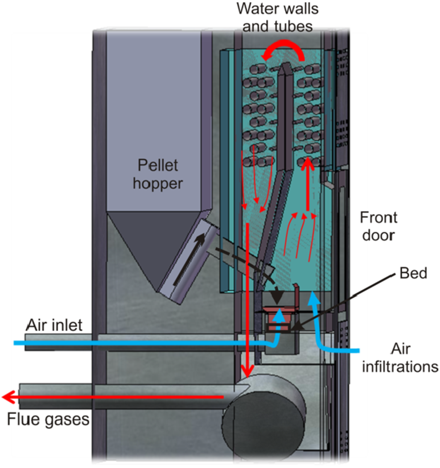
2. Fuel and Experimental Installation

The main parts of the simulated boiler and the movement of the gases and the fuel are illustrated in Figure 1. The fuel particles are introduced into the bed via a feeding screw, which drops the particles into the bed box from the pellet entry placed above. The primary air is divided into two groups of jets; one fraction of the air enters the bed from beneath and the rest enters through several orifices just above the bed, providing a secondary air effect because it is mixed with the gases that leave the bed and feeds the flame. The distribution between these two groups of air streams is set by the geometry of the bed box. A heat exchanger is located over the bed and is formed by two tube banks surrounded by cooled walls. The combustion gases ascend to reach the heat exchanger and then move to the back of the boiler, where an induced fan forces the gases to leave the combustion chamber and enables the boiler to work slightly below atmospheric pressure.

Figure 1. Schematic of the boiler.

Figure 1. Schematic of the boiler.

The boiler is operated at a nominal capacity of 18 kW with a variable air-to-fuel ratio (air excess coefficient) ranging between 2.1 to 3.0 (measured in the chimney), depending on the test performed. Measurements in the air inlet indicate that only approximately one-third of the air enters through this duct and the rest of the air enters via infiltrations that occur at different parts of the freeboard, mostly through the front door, the top cover and an ashtray under the bed. Because the air infiltration values are difficult to measure in each zone, the boundary conditions of the simulation contain some uncertainties that can affect the precision of the results.

The conditions were reproduced in the bed and the air measured by a mass flow meter was imposed at the entrance of the air. The remaining fraction of air needed to attain the air excess was described as infiltration through the door seals, which are not perfectly sealed. The operating conditions and air and fuel flow were maintained for each test; however, the conditions may have varied slightly due to the instantaneous, noncontinuous feeding system of the bed.

Air and exhaust were measured in the primary inlet and in the outlet, respectively, while the fuel feed was adjusted using the regulation system of the boiler. The values for the different measurements have instantaneous variations due to the irregular entry of particles into the bed [15,16].

The fuel characteristics were evaluated using ultimate and proximate analyses and the results are presented in Table 1. Table 2 shows some variables measured in the boiler which were used as boundary conditions in the simulations. As the distribution of the infiltrations is unknown, this distribution was used as an adjustable parameter to obtain good agreement between simulation and experimental results. The air infiltrations were distributed 77% through the ashtray and 23% through the front door. The results obtained during the combustion test are presented in addition to the simulation results in Section 4. Other physical and chemical properties of the pellet can be found in [17].

Table 1. Ultimate and Proximate Analyses of the Fuel Employed (* according to standards ISO 589:2008, ISO 562:2010 and ISO 1171:2010).

Ultimate Analysis		Proximate Analysis *
Carbon [wt %]	52.05	Moisture [wt %]	8.50
Hydrogen [wt %]	6.75	Ash [wt %]	0.62
Oxygen [wt %]	40.97	Fixed Carbon [wt %]	16.20
Nitrogen [wt %]	0.17	Volatile matter [wt %]	74.68
Sulfur [wt %]	0.05	LHV as received [MJ/kg]	18.33

Table 1. Ultimate and Proximate Analyses of the Fuel Employed (* according to standards ISO 589:2008, ISO 562:2010 and ISO 1171:2010).

Ultimate Analysis		Proximate Analysis *
Carbon [wt %]	52.05	Moisture [wt %]	8.50
Hydrogen [wt %]	6.75	Ash [wt %]	0.62
Oxygen [wt %]	40.97	Fixed Carbon [wt %]	16.20
Nitrogen [wt %]	0.17	Volatile matter [wt %]	74.68
Sulfur [wt %]	0.05	LHV as received [MJ/kg]	18.33

Table 2. Measured conditions of the boiler.

Parameter	Simulation Value
Fuel mass flow rate [kg/h]	3.53
Total air mass flow rate [kg/h]	51.40
Air excess ratio [-]	2.25
Primary air mass flow rate [kg/h]	14.81
Total infiltrations mass flow rate [kg/h]	36.59

Table 2. Measured conditions of the boiler.

Parameter	Simulation Value
Fuel mass flow rate [kg/h]	3.53
Total air mass flow rate [kg/h]	51.40
Air excess ratio [-]	2.25
Primary air mass flow rate [kg/h]	14.81
Total infiltrations mass flow rate [kg/h]	36.59

Figure 2. Diagram of the interaction between the bed model and the CFD simulation.

Figure 2. Diagram of the interaction between the bed model and the CFD simulation.

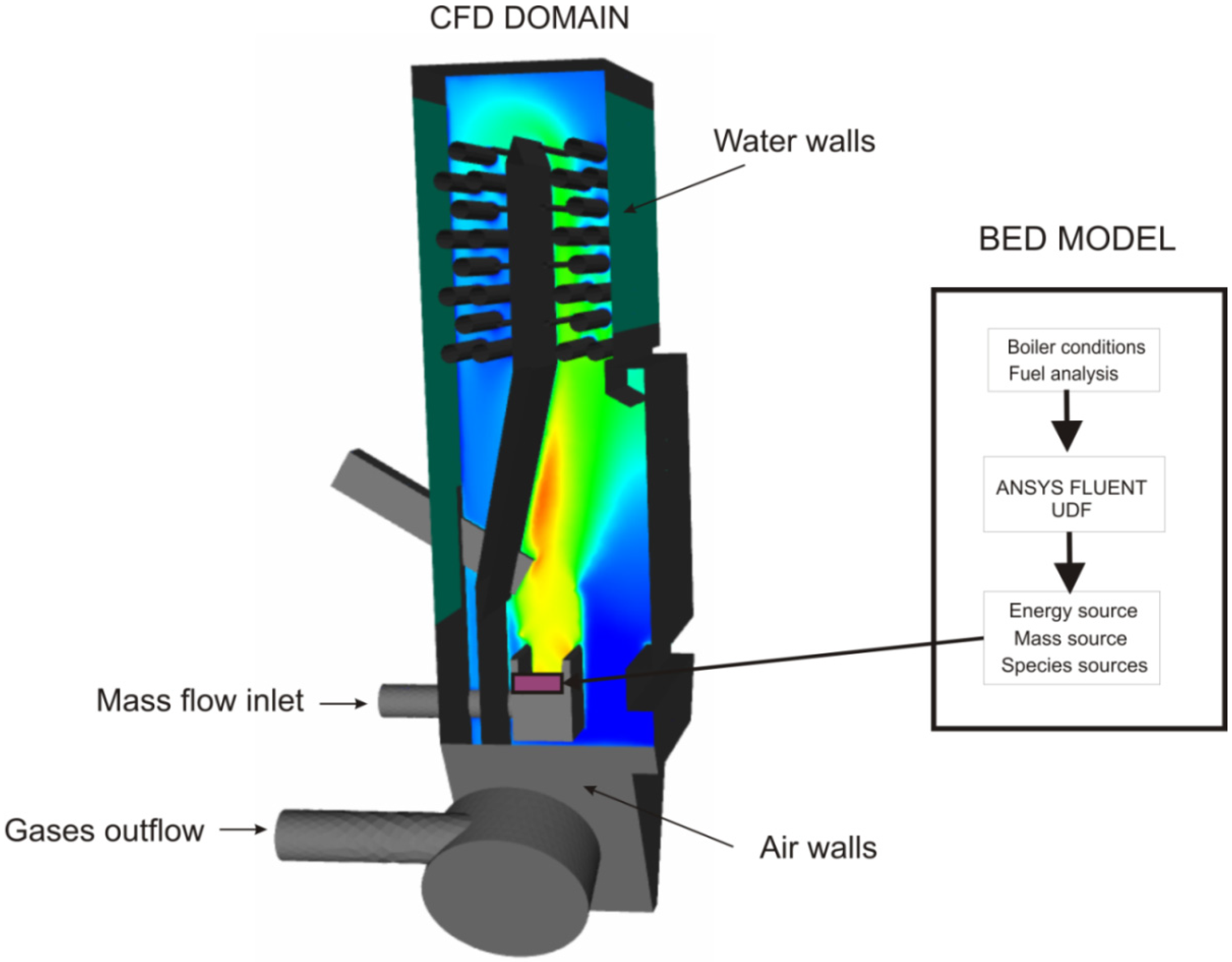
3. Model Description

3.1. Introduction

The entire domain of the boiler can be divided into two zones: the gas zones, where homogeneous reactions, fluid movement and heat transfer occur and the bed, which is part of the gas zones but some mass, energy and species sources are introduced to take into account the biomass combustion process. The interaction between these two zones was externally calculated and coupled to the CFD code through User-Defined Functions (UDFs) programmed in C. The size of the grid was selected to reach grid independence and high accuracy of the variables values. An unstructured three-dimensional tetrahedral grid with approximately 4.5 × 10⁶ elements was chosen. Other grids with approximately 1 × 10⁶ and 8 × 10⁶ elements have been tested and discarded. The first grid did not fulfill the expected accuracy in the results. The computational cost of the second mesh was notably higher and the model showed similar results to those obtained with the chosen mesh. The average size of the element was approximately 5 mm on each side with an average angular skew of 0.3, a maximum angular skew smaller than 0.7 and an average size change of 0.1.

The CFD analysis was based on the commercial code Ansys Fluent 13. Modeling of a biomass boiler involves two main areas of interest: biomass combustion in the bed and homogeneous reactions and heat transfer in the freeboard. The entire fuel bed was included as a portion of the CFD simulation domain and porous media conditions were imposed in the bed volume. The contribution of solids to both energy and mass was programmed in C and was included as a user-defined routine in the commercial code.

3.2. Gas Phase

As in similar works [11,12], the steady-state governing equations were solved using the SIMPLE algorithm; the spatial discretization was solved using the second-order upwind method for the momentum, energy and radiation; and the pressure was determined using PRESTO. The continuity, momentum and energy of the gas phase were modeled according to the standard CFD procedures, which are well documented [13] and will not be discussed in this paper. The realizable k–ε model with enhanced wall treatment was employed to account for the effect of turbulence because of its proven effectiveness in industrial applications [18,19].

Flow through a porous medium was modeled by treating the bed as a homogeneous region with space-averaged properties, which is possible in the commercial CFD code using a porous cell zone in which Ergun’s pressure drop equation is solved (Equation 1). Other parameters, such as viscous and inertial resistance [Equations (2) and (3)], were introduced via UDFs. The mean diameter was calculated from the Rosin-Rammler distribution of the fuel particles:

$$\frac{\mathrm{∆}P}{l_B}=\frac{150 \mu {\left(1-\epsilon \right)}^2}{{d_{eq}}^2 {\epsilon }^3}v+\frac{1.75 {\rho }_g \left(1-\epsilon \right)}{d_{eq} {\epsilon }^3} v^2$$

(1)

$$\alpha =\frac{{\psi }^2{d}_{eq}^2}{150}\frac{{\epsilon }^3}{{\left(1-\epsilon \right)}^2}$$

(2)

$$C_2=\frac{3.5}{\psi d_{eq}}\frac{\left(1-\epsilon \right)}{{\epsilon }^3}$$

(3)

In this study, radiative heat transfer was modeled according to the discrete ordinates model, which solves the radiative transfer equation (RTE) for a finite number of discrete solid angles, each associated with a vector direction $\overrightarrow{s}$ fixed in the global Cartesian system. The absorption coefficient for radiation is calculated as a function of the characteristic cell-size and gas concentrations of the participating gases using the Weighted Sum of Grey Gases Model (WSGGM). Soot is known to play an important role when investigating heat transferred by radiation and its effect was included in the absorption coefficient. The effect of the soot was also included by adding the soot absorption coefficient [Equation (4)], which was calculated using an experimental correlation [20]. The effect of the particles in the bed region, which are assumed to be in thermal equilibrium with the gas phase, is accounted for by adding a solid-phase contribution to the total absorption coefficient [Equation (6)]. The solid-phase absorption coefficient was calculated by considering the diameter of the particles and the porosity of the bed [8]:

$$a_{soot}=0.03 \left(1.6·{10}^{-3} T-0.5\right) \left(2-\lambda \right) \frac{C^R}{H^R} L$$

(4)

$$a_{solid}= -\frac{1}{d }\ln \epsilon$$

(5)

$$a_{total}=a_{gas}+a_{soot}+a_{solid}$$

(6)

3.3. Bed Modeling

Many transport and reaction phenomena occur in the bed of the boiler when the heat from the flame reaches the fuel particles. These processes were modeled by calculating the mass, energy and species generated or consumed when the fuel enters the bed via UDF and by introducing them as sources in the cell zone representing the bed in the simulation. However, some limitations are present when using this bed model because it is performed under perfectly stirred reactor conditions and the particles that form the bed should be treated as being thermally thin. Thermally thin consideration means that heat absorbed by the particle surface will penetrate its thickness rapidly, thus temperature gradient through the particle depth can be neglected [11,21]. The opposite, thermally thick, means that temperature gradient in the particle is relevant [22,23].

The combustion regime of the bed is defined by the Dämkholer number (Da). This dimensionless number relates the mixing time scale with the chemical time scale in the bed. Da was formulated as shown in Equation 7 [11], where $S_b$ is the rate of destruction or generation of gaseous species in the bed, $l_B$ is the bed characteristic length (in this work is represented by the bed height) and $v_0$ is the mean velocity of the gases in the bed:

$$Da=\frac{S_b ·l_B}{\left|\overline{v_0}\right|}=\frac{{\tau }_{conv}}{{\tau }_{reac}}$$

(7)

Because different combustion phases occur simultaneously in different particles, steady state was considered as an average of the entire bed combustion. When the bed is working under steady-state conditions, the rate of destruction or generation of gaseous species in the bed can be estimated by employing the Equation 8, where $\varphi$ is a stoichiometric coefficient of the pellet consumption in the bed. The stoichiometric coefficient relates pellet burning to oxygen consumption, taking into account that only a 20 % of the fuel is the fixed carbon that consumes oxygen in the bed. Its value is approximately 0.53. ${\dot{m}}_f$ is the amount of fuel fed and $V_{bed}$ is the bed volume:

$$S_b=\frac{\varphi ·{\dot{m}}_f}{V_{bed}}$$

(8)

The Dämkholer number calculated with the working conditions of the boiler is approximately 0.1. Therefore, the reaction time is 10 times greater than the residence time, which means that the transport of gases in the bed is enough to consider that almost all the fuel particles in the bed are immersed in gases with similar compositions. Because the process works under well-stirred conditions, the homogeneous behaviour of the bed is imposed in relation to the biomass degradation effects in the gas phase.

The bed was treated as a porous medium in which the solid phase has the same physical properties as the pellets. The composition of the gases emitted does not vary with temperature [24] and was determined by the fuel composition and the conditions assumed for devolatilisation and heterogeneous combustion.

The gas composition was calculated by performing a mass and species balance for each process (drying, pyrolysis and char oxidation) of the fuel combustion. Drying was modeled by releasing the moisture content of the fuel to the gas phase while latent heat of evaporation was removed. The amount of water vapor released by the bed due to the drying process is presented in Equation 9. In a similar manner, volatile species were emitted to the gas phase to simulate the pyrolysis phenomenon. These volatile species are composed mainly of CO, CO₂, H₂, H₂O, NH₃, light hydrocarbons (represented by CH₄) and tars (usually represented by C₆H₆) [25]. Both moistuire and volatile generation rates were calculated from moisture and volatile fractions ($Y_m$ and $Y_v$ respectively) which were deduced from the proximate analysis. The composition of the gases (${\chi }_j$) emitted during devolatilisation was estimated as proposed by Thunman [26]. This composition of gases is variable with the temperature but the variation is not significant between 500 and 700 K which is a typical interval of devolatilisation in biomass. Therefore, a constant temperature of 600 K was employed to estimate the fraction of each one of the volatile gases introduced, whose total amounts were introduced in the gas phase [Equation (10)]. The predicted fractions of the volatile species are listed in the Table 3.

$${\dot{\omega }}_{H_{2}O,m}^{‴}={\dot{\omega }}_f^{‴}{Y}_m$$

(9)

$${\dot{\omega }}_{j,v}^{‴}={\dot{\omega }}_f^{‴}{Y}_v {\chi }_j$$

(10)

Table 3. Fraction of the released volatile species.

Volatile specie (j)	Fraction (${\chi }_j$)
C6H6	0.2883
CH4	0.0256
H2	0.0287
CO	0.1285
CO2	0.3230
H2O	0.2041
NH3	0.0018

Table 3. Fraction of the released volatile species.

Volatile specie (j)	Fraction (${\chi }_j$)
C6H6	0.2883
CH4	0.0256
H2	0.0287
CO	0.1285
CO2	0.3230
H2O	0.2041
NH3	0.0018

Char combustion is a complex process that is affected by the fuel composition, particle shape and boiler conditions. A simplified model was used by Porteiro [11] that considers a heterogeneous reaction of char to form CO and CO₂ [Equation (11)] where $\eta$ is the ratio of the CO/CO₂ formation rate that depends on the temperature [Equation (12)]. A representative char combustion temperature of 1373 K was employed [27] to estimate the composition of the char combustion products, resulting in the expressions in Equations (13) and (14) for CO and CO₂ calculated from char fraction $Y_c$ (value from proximate analysis). The total energy generated or consumed by fuel heating, drying, pyrolysis and char oxidation was also introduced to the CFD code as a source in the energy equation. This source term $S_f$ appears in Equation (15):

$$C+O_2\to 2\left(\eta -1\right)CO+\left(2-\eta \right)C{O}_2$$

(11)

$$\eta =\frac{2\left(1+4.3 e^{\left(\raisebox{1ex}{$-3390$}\!\left/ \!\raisebox{-1ex}{$T$}\right.\right)}\right)}{\left(2+4.3 e^{\left(\raisebox{1ex}{$-3390$}\!\left/ \!\raisebox{-1ex}{$T$}\right.\right)}\right)}$$

(12)

$${\dot{\omega }}_{CO,c}^{‴}={\dot{\omega }}_f^{‴}{Y}_c\frac{2\left(\eta -1\right)}{\eta }$$

(13)

$${\dot{\omega }}_{C{O}_2,c}^{‴}={\dot{\omega }}_f^{‴}{Y}_c\frac{\left(2-\eta \right)}{\eta }$$

(14)

$$S_f={\dot{\omega }}_f^{‴}\left(\left(1-Y_m\right)h_{\text{f}}^0\left(T_{ref},f\right)+Y_m{h}_{\text{f}}^0\left(T_{ref},H_2{O}_{\left(l\right)}\right)-{\displaystyle \sum }_j{\gamma }_j{h}_{\text{f}}^0\left(T_{ref},j\right) \right)$$

(15)

3.4. Combustion Model

A set of chemical reactions was introduced to model the combustion of the species due to the fuel pyrolysis, combustion and gasification processes detailed in the bed modeling section. These reactions consisted of the partial oxidation of benzene [Equation (16)] and methane [Equation (17)] to carbon monoxide. The complete oxidation of hydrogen [Equation (18)] and carbon monoxide [Equation (19)] and the dissociation of carbon dioxide [Equation (20)], which becomes important at high temperatures, complete the homogeneous reactions. The kinetics of the global combustion mechanism of Westbrook and Dryer used by Yin et al. [21] was used to compute the homogeneous reactions. Reasonably good predictions for the major species were obtained using similar oxidation models [28]. Equations (21) and (22) model the combustion of ammonia, which represents the species derived from the nitrogen present in the fuel. The influence of both kinetics and turbulence were accounted for using the Finite-rate/Eddy-dissipation model to compute all of the competitive reactions of the model:

$$C_6{H}_6+\frac{9}{2}{O}_2\to 6 CO+3 H_{2}O$$

(16)

$$C{H}_4+\frac{3}{2} O_2\to CO+2 H_{2}O$$

(17)

$$H_2+\frac{1}{2}{O}_2\to H_{2}O$$

(18)

$$CO+\frac{1}{2}{O}_2\to C{O}_2$$

(19)

$$C{O}_2\to CO+\frac{1}{2}{O}_2$$

(20)

$$N{H}_3+O_2\to NO+H_{2}O+\frac{1}{2}{H}_2$$

(21)

$$N{H}_3+NO\to N_2+H_{2}O+\frac{1}{2}{H}_2$$

(22)

3.5. Heat Transfer

The studied boiler was designed to operate as both a boiler and a stove. Therefore, some of the walls are used to transfer heat to water and others are used to heat the room where the boiler is located. Both heat transfer processes were considered by introducing the appropriate boundary conditions in the walls, which were supposed to be in contact with water and air. These boundary conditions consider convection to water and air and are modeled by selecting the convective coefficients and fluid temperatures. The convective coefficients used were 2500 W m⁻² K⁻¹ and 7 W m⁻² K⁻¹ for water and air, respectively, which are typical values. The measured temperatures in the air walls are reasonably low for not considering the radiation heat loss in the convection coefficient. The air temperature inside the room was set to 20 °C. Because the water temperature was studied to evaluate the boiler performance, different values were used for various simulations and are discussed in the results section. A water temperature of 60 °C was selected for the simulation used for comparison with the experimental data.

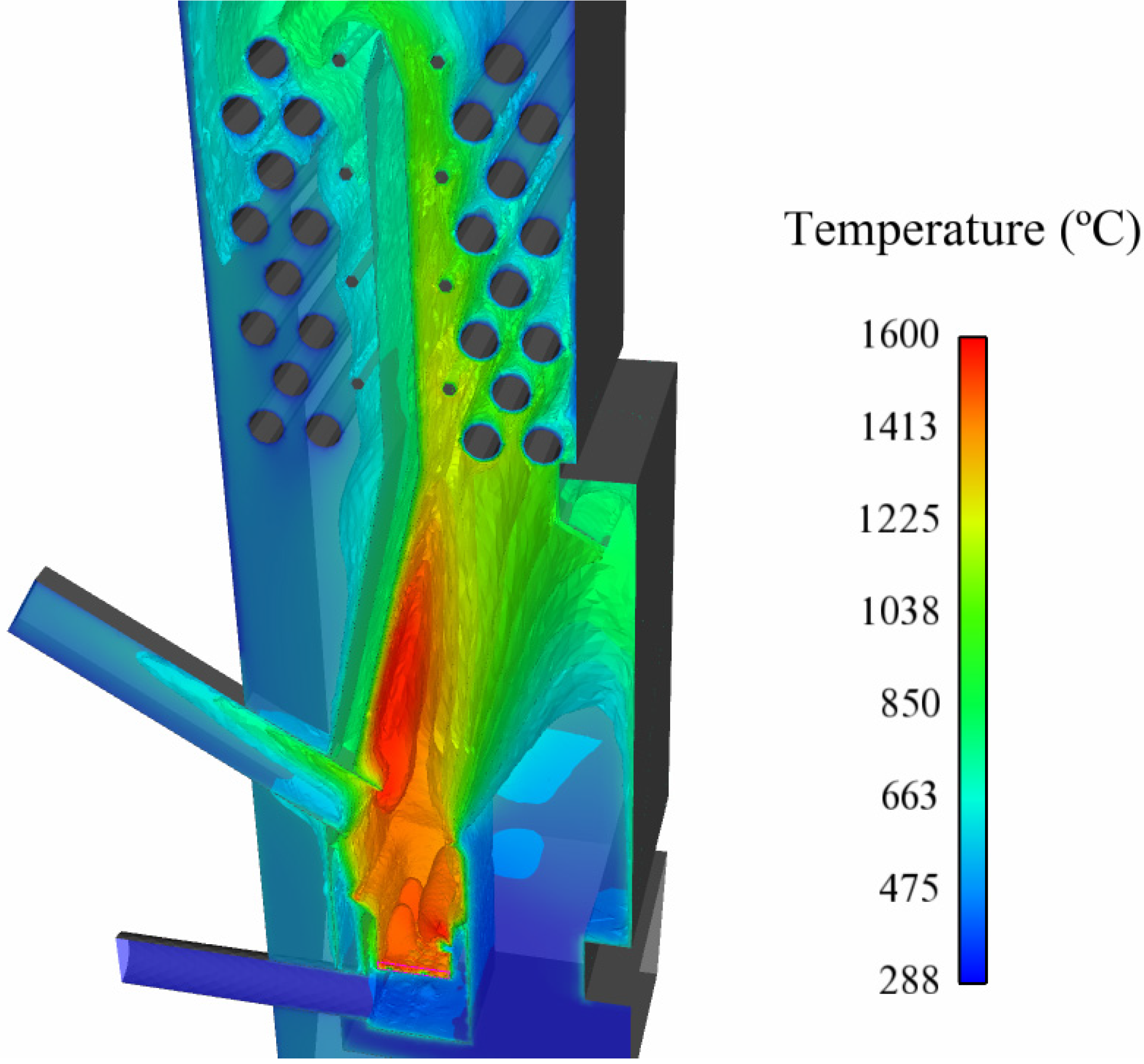
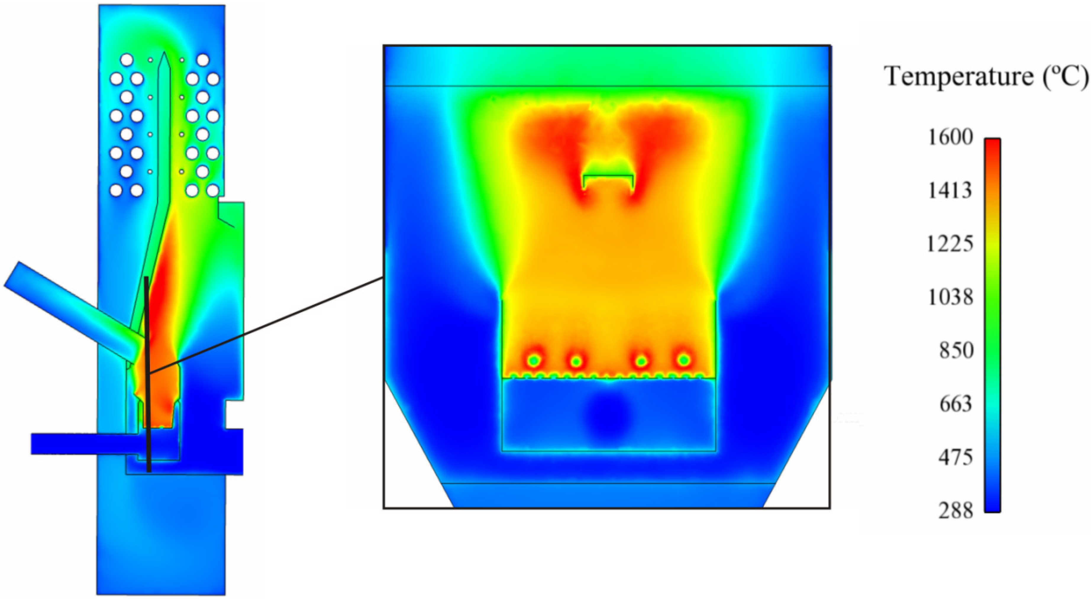
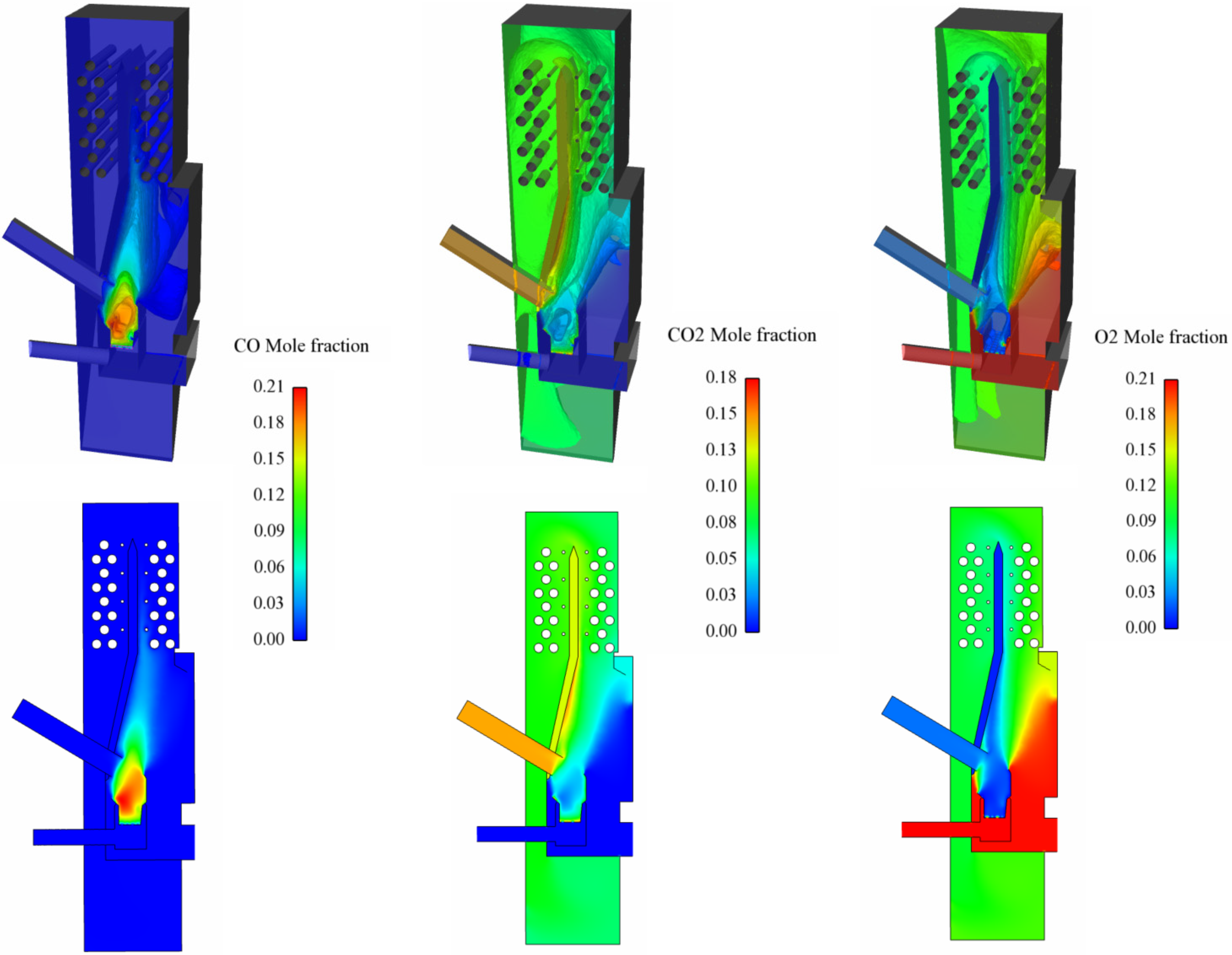
4. Results and Discussion

In the following section, the results of several simulations are analyzed and discussed. First, the results of the proposed model which was applied in a simulation of the boiler under operating conditions, and compared with experimental data to ensure the validity of the proposed model and the assumptions made. The main parameters for the system are then presented and discussed in more depth. Next, the results of a set of simulations in which the water temperature varies are presented to determine the effect of this variation on the key parameters. Finally, various figures are shown to analyze the fields of the main variables inside the boiler.

4.1. Experimental Contrast

Before comparing the CFD results with the measured data, the difficulties of maintaining a constant air-to-fuel ratio (air excess) throughout the tests and measuring gas species in such a combustion system must be understood, especially when considering the commonly high instability of low-power systems [16]. Table 4 presents a comparison between the results of a CFD simulation using the proposed model and the averaged values of the measurements performed after several hours of working continuously. The water temperature in the experimental trials was 60 °C and the air excess coefficient was λ = 2.2; these values were selected because of the resulting higher stability of the boiler. To avoid the influence of uncontrolled dilution during gas composition measurements, the experimental and simulated concentrations refer to the same O₂ concentration (10%) in the flue gases.

Table 4. Comparison between simulation and experimental results.

Parameter	CFD Simulation	Experimental
Heat to water (kW)	13.91	13.31
Outlet temperature (°C)	188.0	174.5
CO2 emissions (%)	9.50	9.92
CO emissions (ppm)	2290	1828
NOx emissions (ppm)	154	256

Table 4. Comparison between simulation and experimental results.

Parameter	CFD Simulation	Experimental
Heat to water (kW)	13.91	13.31
Outlet temperature (°C)	188.0	174.5
CO2 emissions (%)	9.50	9.92
CO emissions (ppm)	2290	1828
NOx emissions (ppm)	154	256

The comparison of the results demonstrated good agreement between the simulated and experimental heat transfer and temperature values. The CO₂ emissions data also showed good agreement with the experimental data and the CO emissions were on the same order of magnitude, despite the simplicity of the combustion and dissociation reaction model. The reasonably good prediction of this model indicates that both the combustion model and the combustion scheme were suitable for this study, considering the large number of processes involved (turbulence, kinetics, mixing and flame quenching) [29]. The predicted NO_x emissions were low in comparison with the experimental measurements; these emissions depend on the fraction of nitrogen, which can vary significantly as a function of fuel heterogeneity.

Some temperature maps of the interior of the freeboard, the bed and the heat exchanger is presented in the Figure 3 and Figure 4. The air that crosses the bed represents only one-third of the air present in the outflow and the air excess is only 2.25, so this air is insufficient to complete the combustion process and the oxygen from the air infiltrations is required. This causes the elongated shape of the flame. Hot areas are observed just over the bed, where the fuel is fed by the primary air and where the air from infiltrations reaches the remaining volatile gases. The flame generated is not completely developed and is interrupted by the water tubes stopping the reactions and contributing to enhance CO emissions; this effect is more pronounced for colder tubes. The maximum temperature reached varies from approximately 1,500 to 1,600 °C, which are typical values for this type of combustion system, as demonstrated in previous works [15,16]. While some tubes are touched by the flame, others are shielded and are reached by cooled gases. In addition, preferred trajectories for the movement of gases are present that favor heat transfer to certain tubes. Figure 4 reveals that the hottest gases move up the central area of the freeboard whose walls are not cooled, which means a loss of efficiency. It also shows temperature gradients in some regions in the bed caused by the entry of the cold air. These contradict the hypothesis of constant temperature in the pyrolysis and the char combustion stages, which is the main weakness of this study.

Figure 5 presents the CO, CO₂ and O₂ mole fraction profiles. CO is more concentrated just over the bed, which is a consequence of the devolatilisation and char oxidation processes [Equation (15)]. Because the primary inlet works under substoichiometric conditions, the volatile hydrocarbon combustion is not completely developed, which provides more CO to the flame [Equations (4) and (5)] and the O₂ from the infiltrations consumes most of the remaining CO.

Figure 3. Gas temperature field (°C) in the freeboard and heat exchanger.

Figure 3. Gas temperature field (°C) in the freeboard and heat exchanger.

Figure 4. Gas temperature (°C) contours of a central axis section and a frontal view of the burner.

Figure 4. Gas temperature (°C) contours of a central axis section and a frontal view of the burner.

CO₂ is not present in the air or infiltration inlets and its concentration increases when char and volatile species react in the bed and freeboard. The opposite process to that used to form CO₂ occurs when the consumed O₂ reacts with the char and volatiles. Therefore, the O₂ concentration is maximum (mole fraction of 0.21) in the air or infiltration inlets and minimum inside the bed and the flame where the volatile species from the pyrolysis react and consume the O₂ from the inlet.

Figure 5. CO, CO₂ and O₂ iso-sufaces and contours of the central axis section of the boiler.

Figure 5. CO, CO₂ and O₂ iso-sufaces and contours of the central axis section of the boiler.

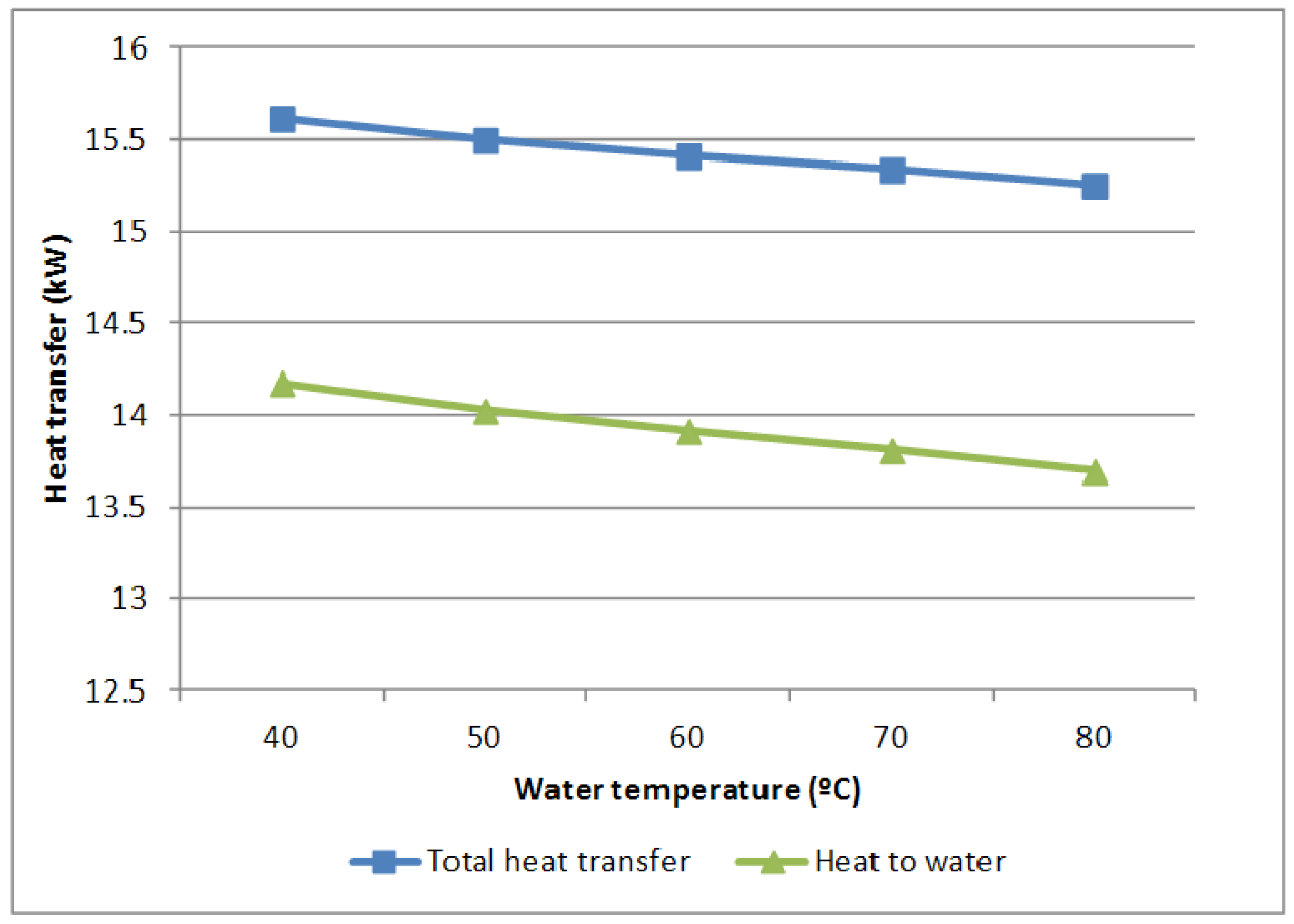
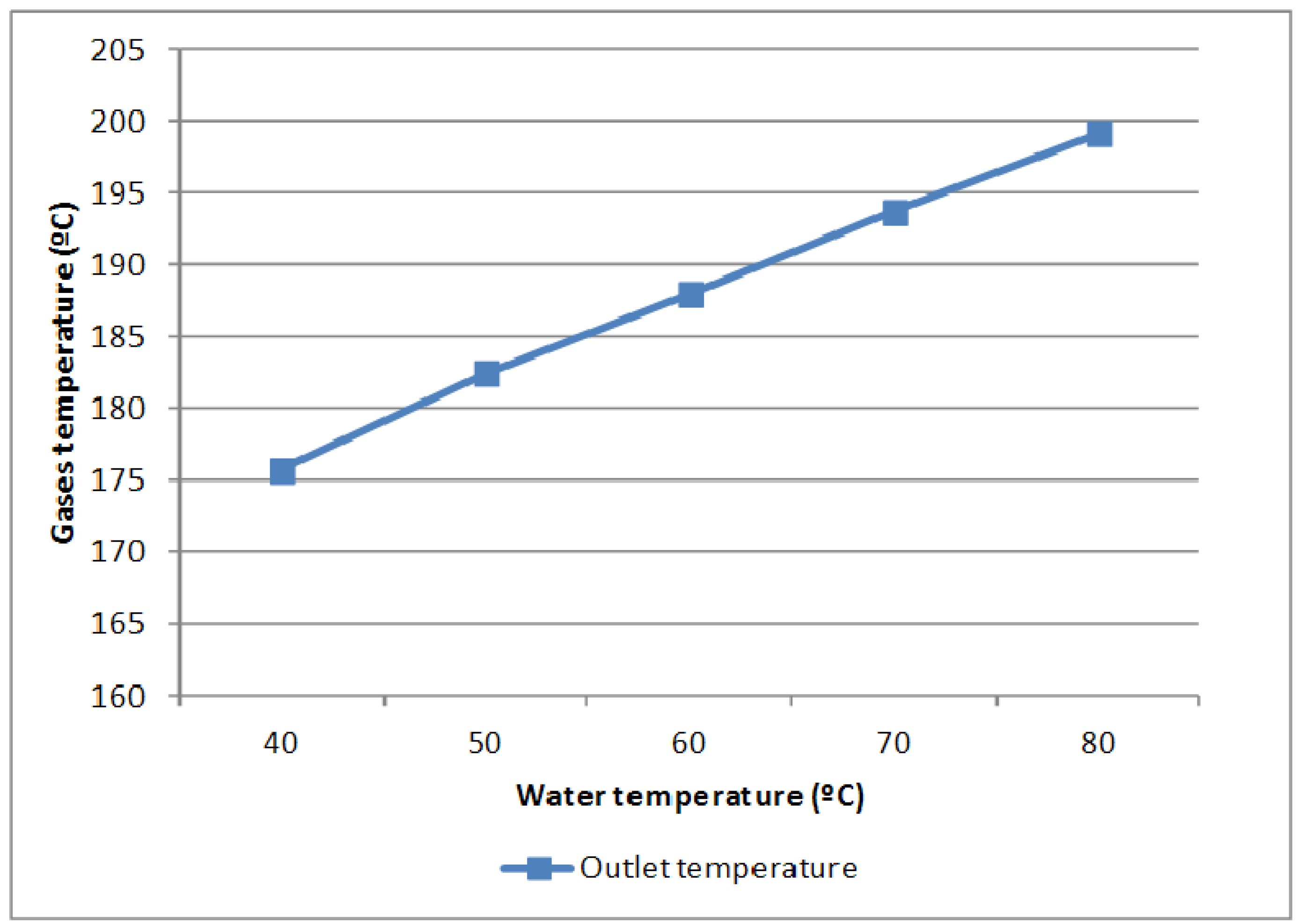
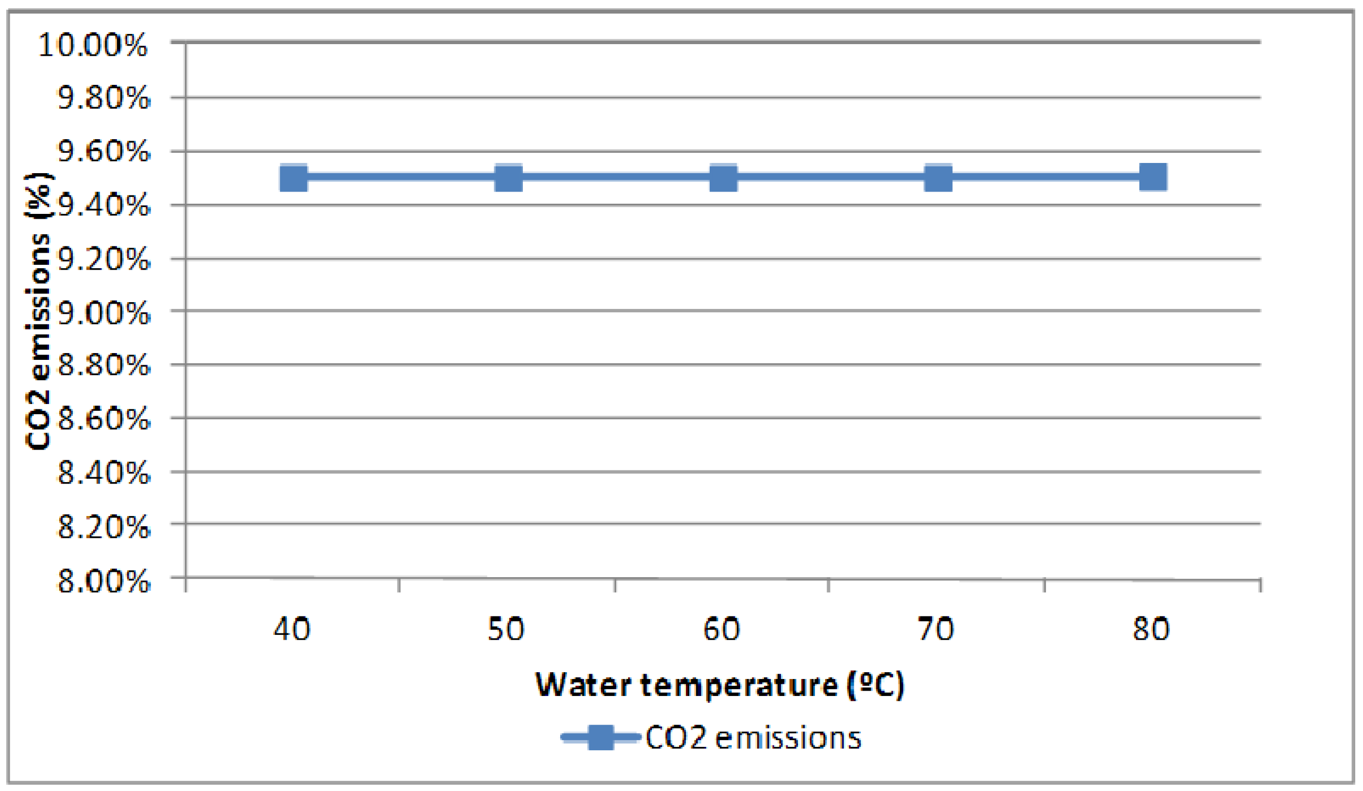
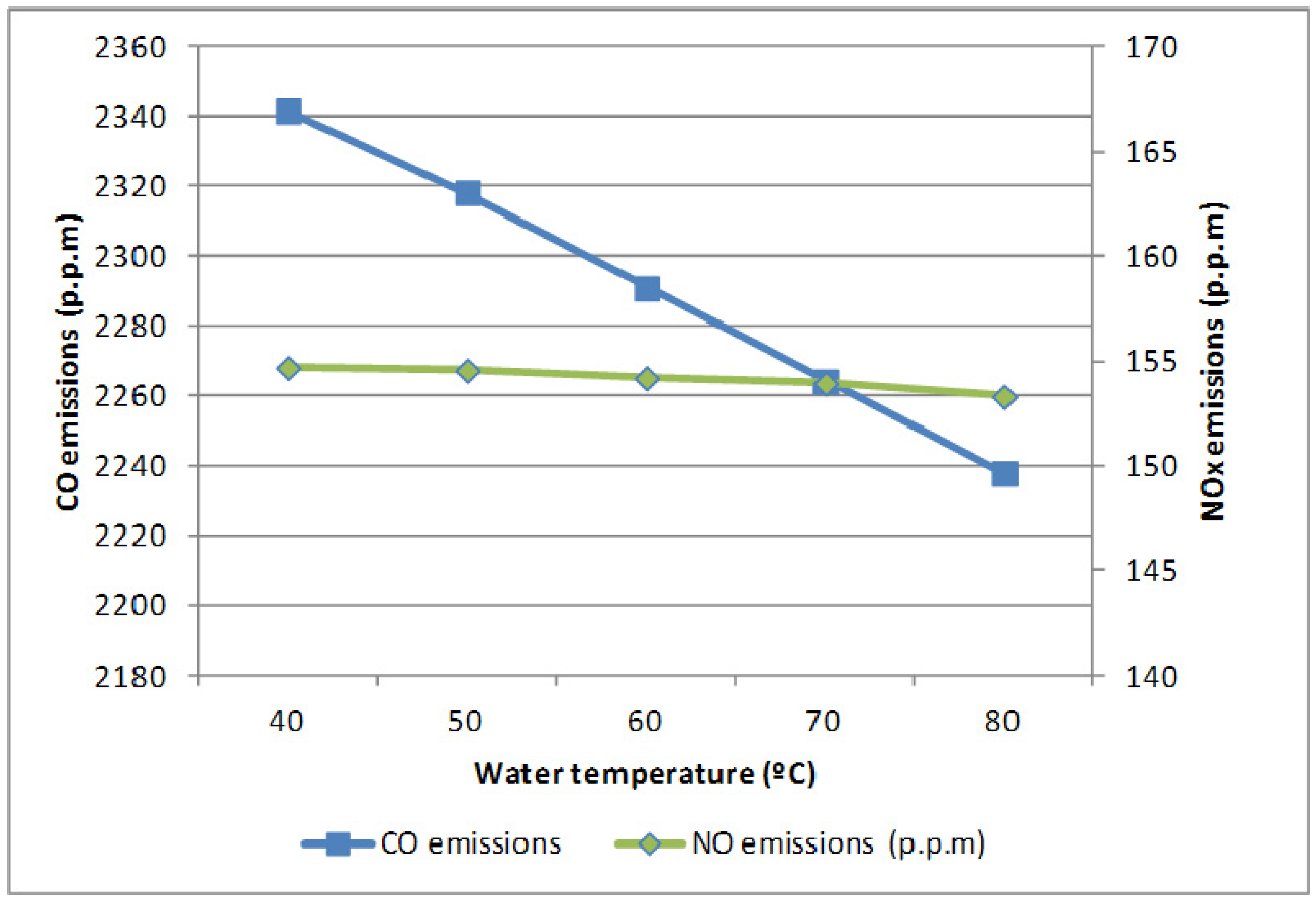
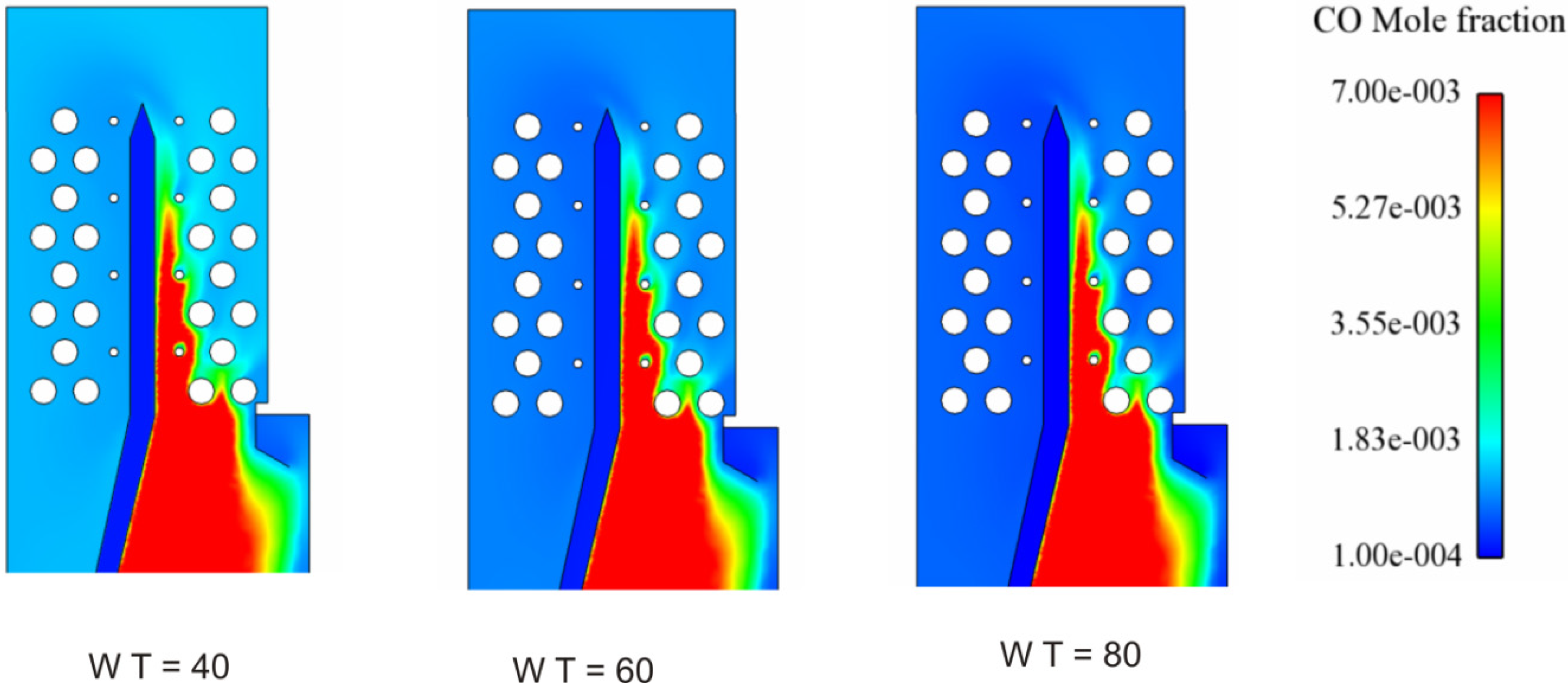
4.2. Water Temperature Effect

The same models and boundary conditions were used to simulate the boiler while varying the water temperature from 40 °C to 80 °C to analyze the effect of these variations on the rest of the parameters. Figure 6 plots the heat supplied to the water and the total heat transfer (water and air) as a function of the water temperature. Although large variations are not observed, the heat transfer has a tendency to increase when the water temperature decreases. The larger temperature gradient in the walls causes this increase in heat transfer; however, because the total variation does not exceed 3% of the total power, the water temperature is revealed to not be a relevant parameter in the heat transfer and, therefore, it is not relevant in the performance of the boiler.

Figure 6. Total heat transfer and heat transfer to water (kW).

Figure 6. Total heat transfer and heat transfer to water (kW).

The predicted temperatures of the flue gases are plotted in Figure 7. The model predicts higher flue gas temperatures when the water temperature increases. This result is caused by the larger heat transfer that occurs when the water temperature is low, which cools the gases in the boiler interior. This gas temperature is an important parameter in controlling acid condensations in the exhaust stacks because biomass contains small concentrations of sulfur.

Figure 7. Temperature of the flue gases (°C).

Figure 7. Temperature of the flue gases (°C).

Figure 8 and Figure 9 illustrate the predicted emissions of pollutants (CO₂ in Figure 8 and CO and NO_x in Figure 9) in the flue gases. Because the experimental concentrations were calculated with respect to 10% O₂, the predicted values of the simulations were also calculated using the same O₂ concentration. The CO₂ content remained constant over the entire water temperature range; however, the simulation captured a decrease of CO from the exhaust with increasing water temperature. Most CO emissions in combustion systems typically appear due to flame quenching at the walls. If the flame touches a cold surface, gaseous reactions are halted and because CO acts as an intermediate product in the complete combustion to CO₂, a fraction of that CO remains. This phenomenon is more pronounced the lower the temperature of the walls. The NO_x fraction is almost constant over this temperature range.

Figure 8. Predicted CO₂ emissions.

Figure 8. Predicted CO₂ emissions.

Figure 9. Predicted CO and NO_x emissions.

Figure 9. Predicted CO and NO_x emissions.

Figure 10 presents the predicted distribution of the molar fraction of CO inside the boiler. The scale is in a reduced range which allows appreciating the differences in CO concentrations. All the simulations predict similar CO concentrations in the flame (red colour in the contours, which means a CO mole fraction greater than 7 × 10⁻³); however, higher concentrations of CO appear in the lower water temperature simulations when the gases pass through the heat exchanger. The upper area of the flame is reached by the air from the infiltrations at the front of the boiler, which consume the CO. However, a portion of the gas mixture is cooled by the refrigerated walls, preventing the oxidation reactions. These results indicate that the position of the water tubes, the distribution of the air inlets and the air infiltrations are the key factors determining the high emission levels in this type of system.

Figure 10. CO mole fraction contours with different water temperatures (W T) in the heat exchanger.

Figure 10. CO mole fraction contours with different water temperatures (W T) in the heat exchanger.

5. Conclusions

A simple approach to simulating biomass boilers whose beds can be assumed to be perfectly mixed is presented in this paper. This modeling method and its application to a commercial case was performed using experimental data.

The method presents some weaknesses such as the assumption of constant temperatures for the calculation of pyrolysis and char oxidation products. This simplification is not relevant in this simulation because the bed dimensions, especially depth, are small in comparison with the freeboard dimensions. However, the local bed temperature should be considered in simulations with larger beds.

Despite the simplicity of the methodology and the assumptions of the model, the predictions and the main behavior of the system seem to be correct because the results obtained with this model have an acceptable level of accuracy when compared with experimental measurements. The porous bed combustion mechanism, coupled with the CFD simulation of the combustion chamber via UDFs, appears to be adequately formulated and solved. Overall, the boiler efficiency and main emissions were correctly predicted, except for the NO_x emissions, whose predicted values are too low compared with the experimental data.

The methodology presented was used to simulate and analyze the influence of the water temperature on the performance and emissions of the studied boiler. The results indicate that low water temperatures increase the heat transfer with a corresponding increase in performance. However, this increase also leads to increases in CO emissions. These results can be extrapolated to similar systems involving the low-power combustion of solid fuels.

The results can significantly help to improve and optimize biomass combustion system designs. However, validation of these types of models through a comparison with detailed experimental tests must still be performed.

References

1. Dinh Tung, N.; Steinbrecht, D.; Vincent, T. Experimental Investigations of Extracted Rapeseed Combustion Emissions in a Small Scale Stationary Fluidized Bed Combustor. Energies 2009, 2, 57–70. [Google Scholar]
2. Demirbas, M.F.; Balat, M.; Balat, H. Potential contribution of biomass to the sustainable energy development. Energy Convers. Manag. 2009, 50, 1746–1760. [Google Scholar] [CrossRef]
3. Saastamoinen, J. Modelling of Wood Combustion in Small Stoves. In Proceedings of Nordic Workshop on Combustion of Biomass, Trondheim, Norway, February 1991.
4. Ghenai, C.; Janajreh, I. CFD analysis of the effects of co-firing biomass with coal. Energy Convers. Manag. 2010, 51, 1694–1701. [Google Scholar] [CrossRef]
5. Yang, Y.B.; Sharifi, V.N.; Swithenbank, J.; Ma, L.; Darvell, L.I.; Jones, J.M.; Pourkashanian, M.; Williams, A. Combustion of a single particle of biomass. Energy Fuels 2008, 22, 306–316. [Google Scholar] [CrossRef]
6. Peng, Z.; Liu, B.; Wang, W.; Lu, L. CFD investigation into diesel PCCI combustion with optimized fuel injection. Energies 2011, 4, 517–531. [Google Scholar] [CrossRef]
7. Yin, C.; Rosendahl, L.A.; Kær, S.K. Grate-firing of biomass for heat and power production. Progr. Energy Combust. Sci. 2008, 34, 725–754. [Google Scholar] [CrossRef]
8. Shin, D.; Choi, S. The combustion of simulated waste particles in a fixed bed. Combust. Flame 2000, 121, 167–180. [Google Scholar] [CrossRef]
9. Yin, C.; Rosendahl, L.; Kær, S.K.; Clausen, S.; Hvid, S.L.; Hiller, T. Mathematical modeling and experimental study of biomass combustion in a thermal 108 MW grate-fired boiler. Energy Fuels 2008, 22, 1380–1390. [Google Scholar] [CrossRef]
10. Zhang, X.; Chen, Q.; Bradford, R.; Sharifi, V.; Swithenbank, J. Experimental investigation and mathematical modelling of wood combustion in a moving grate boiler. Fuel Process. Technol. 2010, 91, 1491–1499. [Google Scholar] [CrossRef]
11. Porteiro, J.; Collazo, J.; Patiño, D.; Granada, E.; Gonzalez, J.C.M.; Míguez, J.L. Numerical modeling of a biomass pellet domestic boiler. Energy Fuels 2009, 23, 1067–1075. [Google Scholar] [CrossRef]
12. Comesaña, R.; Collazo, J.; Míguez, J.L.; Porteiro, J. CFD Simulation of a Fixed Bed 60 kW Biomass Boiler. In Proceedings of the 18th European Biomass Conference and Exhibition, Lyon, France; 2010; pp. 1327–1331. [Google Scholar]
13. Ansys Fluent 12.0 Theory Guide, 2009. Available online: https://www.sharcnet.ca/Software/Fluent12/html/th/main_pre.htm (accessed on 18 April 2012).
14. Ansys Fluent 12.0 UDF Manual, 2009. Available online: https://www.sharcnet.ca/Software/Fluent12/pdf/udf/fludf.pdf (accessed on 18 April 2012).
15. Moran, J.C.; Granada, E.; Porteiro, J.; Míguez, J.L. Experimental modelling of a pilot lignocellulosic pellets stove plant. Biomass Bioenergy 2004, 27, 577–583. [Google Scholar] [CrossRef]
16. Morán, J.C.; Tabarés, J.L.; Granada, E.; Porteiro, J.; López-González, L.M. Effect of different configurations on small pellet combustion systems. Energy Sources Part A Recovery Utilizat. Environ. Effects 2006, 28, 1135–1148. [Google Scholar] [CrossRef]
17. Porteiro, J.; Patiño, D.; Collazo, J.; Granada, E.; Moran, J.C.; Miguez, J.L. Experimental analysis of the ignition front propagation of several biomass fuels in a fixed-bed combustor. Fuel 2010, 89, 26–35. [Google Scholar] [CrossRef]
18. Sumner, J.; Watters, C.S.; Masson, C. CFD in wind energy: The virtual, multiscale wind tunnel. Energies 2010, 3, 989–1013. [Google Scholar] [CrossRef]
19. Zahirović, S.; Scharler, R.; Kilpinen, P.; Obernberger, I. Validation of flow simulation and gas combustion sub-models for the CFD-based prediction of NOx formation in biomass grate furnaces. Combust. Theory Modell. 2011, 15, 61–87. [Google Scholar] [CrossRef]
20. A.G. Blokh. Heat Transfer in Steam Boiler Furnaces, 1st ed.; Hemisphere Publishing Corporation: New York, NY, USA, 1988. [Google Scholar]
21. Yin, C.; Kær, S.K.; Rosendahl, L.; Hvid, S.L. Co-firing straw with coal in a swirl-stabilized dual-feed burner: Modelling and experimental validation. Bioresour. Technol. 2010, 101, 4169–4178. [Google Scholar] [CrossRef] [PubMed]
22. Gubba, S.R.; Ma, L.; Pourkashanian, M.; Williams, A. Influence of particle shape and internal thermal gradients of biomass particles on pulverised coal/biomass co-fired flames. Fuel Process. Technol. 2011, 92, 2185–2195. [Google Scholar] [CrossRef]
23. Yang, Y.B.; Sharif, V.N.; Swithenbank, J. Numerical simulation of the burning characteristics of thermally-thick biomass fuels in packed-beds. Process Safety Environ. Protect. 2005, 83, 549–558. [Google Scholar] [CrossRef]
24. Girgis, E.; Hallett, W.L.H. Wood combustion in an overfeed packed bed, including detailed measurements within the bed. Energy Fuels 2010, 24, 1584–1591. [Google Scholar] [CrossRef]
25. Bryden, K.M.; Ragland, K.W. Numerical modeling of a deep, fixed bed combustor. Energy Fuels 1996, 10, 269–275. [Google Scholar] [CrossRef]
26. Thunman, H.; Niklasson, F.; Johnsson, F.; Leckner, B. Composition of volatile gases and thermochemical properties of wood for modeling of fixed or fluidized beds. Energy Fuels 2001, 15, 1488–1497. [Google Scholar] [CrossRef]
27. Porteiro, J.; Patiño, D.; Moran, J.; Granada, E. Study of a fixed-bed biomass combustor: Influential parameters on ignition front propagation using parametric analysis. Energy Fuels 2010, 24, 3890–3897. [Google Scholar] [CrossRef]
28. Hermansson, S.; Thunman, H. CFD modelling of bed shrinkage and channelling in fixed-bed combustion. Combust. Flame 2011, 158, 988–999. [Google Scholar] [CrossRef]
29. Collazo, J.; Porteiro, J.; Patiño, D.; Miguez, J.L.; Granada, E.; Moran, J. Simulation and experimental validation of a methanol burner. Fuel 2009, 88, 326–334. [Google Scholar] [CrossRef]