A Low-Carbon Dispatch Model in a Wind Power Integrated System Considering Wind Speed Forecasting and Energy-Environmental Efficiency

Abstract

This paper introduces the “Energy-Environmental Efficiency” concept of building a low-carbon dispatch model of wind-incorporated power systems from the perspective of environmental protection and low-carbon dispatch promotion based on the existing economic environmental dispatch. A rolling auto-regressive and moving-average model is adopted to forecast wind speeds for the next 24 h and reduce the disadvantages brought about to the power system dispatch by wind speed fluctuations. A fuzzy satisfaction-maximizing approach is employed to convert the multi-objective decision-making problem in the low-carbon dispatch model into a single nonlinear one. Particle swarm optimization with a simulated annealing algorithm hybrid is used for better solutions. Simulation results show that the energy-environmental efficiency concept benefits the optimization of the proposed power system dispatch, and the proposed low-carbon dispatch model is reasonable and practical.

1. Introduction

The global energy security and environment situation has become increasingly serious in recent years, leading to a mounting social appeal for environmental protection and sustainable development [1]. One of the most promising nonpolluting renewable energy sources, wind power, has been given more consideration by policies because of its difference from conventional energy sources [2]. Wind power in China has developed in leaps and bounds in recent years. The total wind power capacity of China at the end of 2010 has reached 44,734 MW, exceeding the United States for the first time and ranking first in the World [3]. A zero-emission carbon dioxide renewable resource, wind power is expected to optimize the power source structure, and to promote energy savings and emission reduction in the power industry through large-scale research and development. However, unlike conventional power generation, wind power generation is intermittent and fluctuating. Hence, its integration brings several problems to the power system, dispatch operation being one of the most important aspects [4,5,6,7].

The intermittent and unpredictable nature of wind power generation can influence generation schedule and frequency control. For this reason, the main method currently used to deal with problems of grid-connected wind power generation is to integrate wind speed forecasting into dispatch operation. Real-time regulation of grid dispatch strategy based on wind speed and wind power forecasting can alleviate the adverse effects caused by wind integration to the grid, increase wind power penetration limits, and reduce power system operation costs. Current wind power forecast methods could be divided into two categories based on energy transformation perspective. The first is indirect methods, which provide wind speed forecasts followed by calculation of the output power of wind farm based on the wind speed-power function curve. The second is direct methods, which directly predict the output power of wind via historical wind power data. Generally, the predicted results will change along with the strength of object regularity. The strength of the regularity of the wind power is weaker than that of the wind speed. Hence, indirect methods can reflect the random fluctuation of wind speed more reasonably than direct methods and are also widely used in wind power prediction. 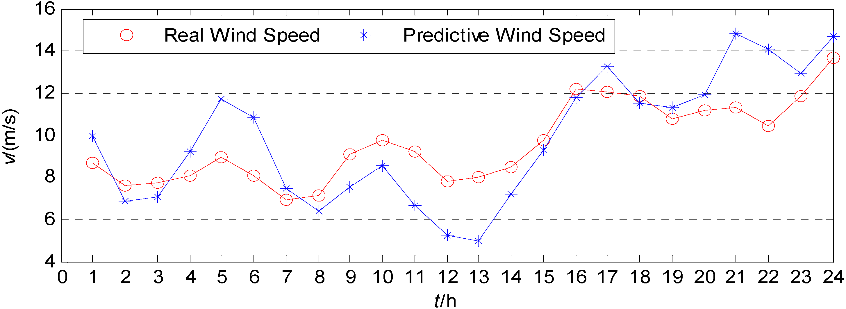Wind speed forecasting is classified into very short-term, short-term, and medium- and long-term forecasting [8], The error of very short-term forecasting (on the minutes or seconds range) is generally between 5% and 10% [9], while short-term forecasting (for the next 24 h) generally has an average prediction error varying from 25% to 40% [10]. Auto-regressive and moving-average (ARMA), artificial neural network, Kalman filter algorithm, fuzzy logic, and wavelet analysis are the most commonly used methods in wind speed forecasting. However, these methods mainly aim at very short-term forecasting, without considering the time sequence of wind speed data. A fairly accurate short-term forecasting is critical to optimal power system load dispatch. Obtaining such forecasts, typically for the next 24 h, will enable the dispatch department to ensure timely planning and regulation of the dispatch schedule, and thus improve significantly the security and economy of the power system.

The power industry is a major CO₂-emission source, accounting for approximately 40% of the CO₂ emitted by fossil fuel combustion. In many important energy-consuming countries such as the United States, China, and Australia, fossil fuels will serve as the main domestic sources of power generation in the next few decades [11,12]. The Kyoto Protocol stipulates that greenhouse gas emission reduction targets must be realized by 2012, which leaves many countries under severe pressure to achieve CO₂ emission reductions. With the deterioration of environmental pollution and the energy crisis, and under the premise of large-scale wind power integration, optimization scheduling can effectively reduce CO₂ emissions, promote low carbon for power production, and promote sustainable development in the power industry.

The traditional power system economic dispatch (ED) is usually aimed at minimum generation operational cost [13,14,15,16] for economic reasons, overlooking the effect of consequent pollutants on the ecosystem. With increasing public awareness of environmental pollution caused by fossil fuels, the traditional ED cannot satisfy the strategic requirements for sustainable living because of the excessive amount of emission pollution [17]. As an alternative, the environmental/ED (EED) is becoming increasingly desirable for minimizing cost and emission [18,19,20]. Reference [21] developed an improved Hopfield neural network for the EED problem. Cai et al. [22] solved the EED problems considering both economic and environmental issues using a multi-objective chaotic particle swarm optimization (PSO). Chena and Chen [23] presented a direct Newton-Raphson method based on an alternative Jacobian matrix to solve the EED problem with line flow constraints. Cheng [24] proposed a multi-objective dispatch that considers environment and fuel cost under large wind energy. Ummels et al. [25] proposed a new simulation method that can fully assess the effects of large-scale wind power on system operations from the cost, reliability, and environmental perspectives.

Based on the ED and EED models, the present paper focuses on the low carbonization of the power system dispatch while maintaining moderate interest in the power generation economy from an ecological perspective. The energy-environmental efficiency concept is introduced into the optimal dispatch of wind-incorporated power systems, for which a low-carbon dispatch model considering unit commitment is built based on wind speed prediction. This paper is organized as follows: Section 1 provides an introduction. 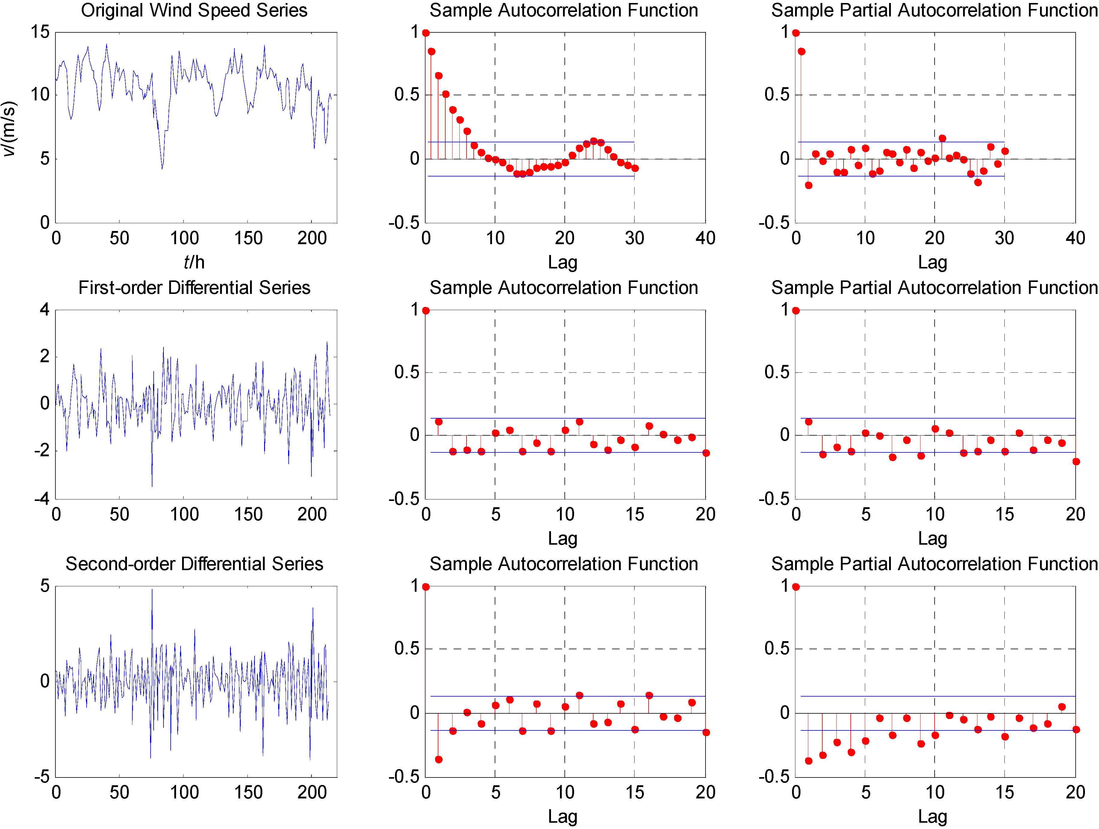Section 2 presents the ARMA-based wind speed forecasting approach and the wind speed-power function of wind generators is presented. Data analysis is also conducted on the field wind speed data of a certain wind farm. In Section 3, a low-carbon dispatch model considering energy-environmental efficiency is described. Section 4 introduces the basic PSO algorithm and the simulated annealing (SA) algorithms. The PSO with SA (PSO-SA) hybrid algorithm is presented to overcome the inherent defects in the PSO and SA algorithms, and to achieve optimized performance. 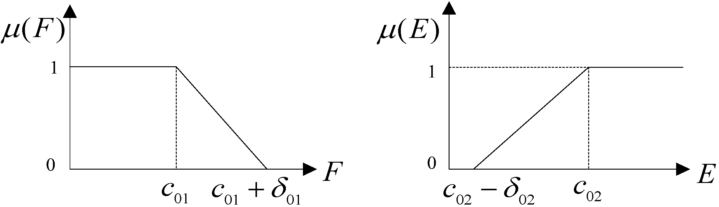In Section 5, the fuzzification method and the concrete calculation steps are pointed out for the aforementioned dispatch model. Section 6 analyzes the results of a six-generator system containing a wind farm. Finally, conclusions are drawn and discussed in Section 7.

2. Wind Speed and Generated Power Forecasting in Wind Farm

2.1. Wind Speed Forecasting Based on Time Series

Time series, which contains data series and data size at the same time, presents a dynamic process of the physical world and reflect the objective world and its changing information. Wind speed data in the wind farm have the characteristics of sequence and discretization. The greatest advantage of time series analysis modeling is that the time series itself and its correlation provide enough information [26]. As long as a limited sample series is provided, a forecasting model with high precision can be built. Based on the abovementioned advantages, the present paper employs the time series method for wind speed forecasting.

2.1.1. Time Series Models

The time series model is built based on the stationarity hypothesis of random series. The most widely used models are the autoregressive (AR) model, the moving average (MA) model, and the ARMA model. The AR and MA models can be transformed from each other while ARMA is the combination of the former two [27]. The characteristics of the three models are listed in Table 1.

Table 1. Characteristics of time series models.

Model type	AR (p)	MA (q)	ARMA (p, q)
Autocorrelation	Tail-off	Cut-off	Tail-off
Partial autocorrelation	Cut-off	Tail-off	Tail-off

Table 1. Characteristics of time series models.

Model type	AR (p)	MA (q)	ARMA (p, q)
Autocorrelation	Tail-off	Cut-off	Tail-off
Partial autocorrelation	Cut-off	Tail-off	Tail-off

The ARMA model can be expressed as:

$${\tilde{Z}}_t={\phi }_1{\tilde{Z}}_{t-1}+\cdots +{\phi }_p{\tilde{Z}}_{t-p}+a_t-{\theta }_1{a}_{t-1}-\cdots -{\theta }_q{a}_{t-q}$$

(1)

Equation (1) can be further transformed into:

$$\phi (B){\tilde{Z}}_t=\theta (B)a_t$$

(2)

where $\left\{{\tilde{Z}}_t\right\}$ represents the time series of the random variables under consideration, whose average is zero and satisfies stationarity; {a_t} is the white noise sequence whose average is zero and variance is ${\sigma }_{\mathrm{a}}^2$; φ_i (i = 1, 2, …, p) is the AR coefficient; θ_j (j = 1, 2, …, q) is the MA coefficient; and B is the backward shifting operator defined as:

$$B{\tilde{Z}}_t={\tilde{Z}}_{t-1},B^j{\tilde{Z}}_t={\tilde{Z}}_{t-j}$$

(3)

When q = 0, the ARMA (p, q) model is converted to the AR (p) model; when p = 0, the ARMA (p, q) model is changed to the MA (q) model. In practice, time series models are usually not stable (wind speed for example). In this case, stationarization is required for modeling. Differentiation is an easy but effective way to implement stationarization. Based on the above analysis, a non-stationary time series model, the AR-integrated MA (ARIMA) model, can be built. The ARIMA is expressed as:

$${\phi }^{\prime }(B){\tilde{Z}}_t=\theta (B)a_t$$

(4)

where ${\phi }^{\prime }(B){\tilde{Z}}_t=\phi (B){(1-B)}^d{\tilde{Z}}_t=\phi (B){\nabla }^d{\tilde{Z}}_t$, $\nabla =1-B$ is the backward differential evolution operator.

2.1.2. Parameter Estimation

The parameters of the ARMA (p, q) model, φ_i, θ_j, and ${\sigma }_{\mathrm{a}}^2$, are estimated by the moment estimation method. The estimation steps are as follows:

(1) AR coefficient estimation

Based on the Yule-Walker equation:

$${\gamma }_A={\gamma }_B\phi$$

(5)

From Equation (5), the estimation expression of the AR coefficient φ_i can be deducted as:

$$\phi ={\gamma }_B^{-1}{\gamma }_A$$

(6)

where φ is the AR coefficient vector, ${\gamma }_A$ is the auto-covariance function vector, and ${\gamma }_B$ is the auto-covariance function matrix. Their respective concrete expressions are as follows:

$$\phi =\left[\begin{array}{c}{\widehat{\phi }}_1\\ {\widehat{\phi }}_2\\ ⋮\\ {\widehat{\phi }}_p\end{array}\right]\begin{array}{cc},& {\gamma }_A=\left[\begin{array}{c}{\widehat{\gamma }}_{q+1}\\ {\widehat{\gamma }}_{q+2}\\ ⋮\\ {\widehat{\gamma }}_{q+p}\end{array}\right]\end{array}\begin{array}{cc},& {\gamma }_B=\left[\begin{array}{cccc}\begin{array}{c}{\widehat{\gamma }}_q\\ {\widehat{\gamma }}_{q+1}\\ ⋮\\ {\widehat{\gamma }}_{q+p-1}\end{array}& \begin{array}{c}{\widehat{\gamma }}_{q-1}\\ {\widehat{\gamma }}_q\\ ⋮\\ {\widehat{\gamma }}_{q+p-2}\end{array}& \begin{array}{c}{\widehat{\gamma }}_{q-2}\\ {\widehat{\gamma }}_{q-1}\\ ⋮\\ {\widehat{\gamma }}_{q+p-3}\end{array}& \begin{array}{c}{\widehat{\gamma }}_{q-p+1}\\ {\widehat{\gamma }}_{q-p+2}\\ ⋮\\ {\widehat{\gamma }}_q\end{array}\end{array}\right]\end{array}$$

(7)

(2) To estimate the MA coefficients θ_j and ${\sigma }_a^2$

Let y_t be:

$$y_t={\tilde{Z}}_t-{\widehat{\phi }}_1{\tilde{Z}}_{t-1}-\cdots -{\widehat{\phi }}_p{\tilde{Z}}_{t-p}$$

(8)

From Equations (1) and (8), y_t can be deducted as:

$$y_t\approx a_t-{\theta }_1{a}_{t-1}-\cdots -{\theta }_q{a}_{t-q}$$

(9)

The model described by Equation (9) can be viewed as the MA (q) process. The following equation set is solved:

$${\widehat{\gamma }}_{y,k}=\{\begin{array}{ll}{\widehat{\sigma }}_a^2(1+{\widehat{\theta }}_1^2+{\widehat{\theta }}_2^2+\cdots +{\widehat{\theta }}_q^2),& k=0\\ {\widehat{\sigma }}_a^2(-{\widehat{\theta }}_k+{\widehat{\theta }}_1{\widehat{\theta }}_{k+1}+\cdots +{\widehat{\theta }}_{q-k}{\widehat{\theta }}_q),& k=1,2,\cdots ,q\end{array}$$

(10)

where ${\widehat{\gamma }}_{y,k}$ is the auto-covariance coefficient of sequence {y_t}.

Equation (10) can be solved by the direct method (suitable for q < 3), the linear iteration method, and the Newton–Raphson algorithm. In the present paper, moment estimations θ_j and ${\sigma }_a^2$ are obtained by a combination of the linear iteration method and the direct method to solve Equation (10).

2.1.3. Model Order Determination

The partial correlation order determination method and the criterion function order determination method are often used to determine model order. Considering the simplicity principle of modeling, the values of p and q are relatively small in practice. Thus, the exhaustion method is also applicable in model selection. Moreover, not all the results by the criterion function order determination are accurate in the calculation process. Therefore, the present paper carries out each model determination one by one, from the lower order to the higher order, by fitting and examination using the partial correlation order determination method for reference.

2.1.4. Model Examination

Model examination involves two aspects: (1) stationarity and reversibility examination and (2) residual error examination. The condition for parameters to meet the stationary requirement is “no root of the characteristic equation of the coefficient φ(B) = 1 − φ₁B − φ₂B² − … − φ_pB^p = 0 is within the unit circle (i.e., the modulus of the roots all bigger than one).” The condition for parameters to meet the reversibility requirement is “no root of the characteristic equation of the coefficient θ(B) = 1 − θ₁B − θ₂B² − … − θ_qB^q = 0 is within the unit circle.” The objective of inspecting the model’s residual error is to judge whether the fitting residual sequence {a_t} is white noise or not [28]. If it is, then this model can be accepted; otherwise, the model needs rebuilding. The criterion of the residual error examination is the slight difference between auto-covariance function and zero.

2.1.5. Rolling Time Series Forecasting Method

The ARMA model in this paper uses a single-step prediction method with a time interval of 1 h to obtain an hour-ahead-of-time wind speed forecast. As the dispatching department generally requires multi-step prediction results 1~3 h ahead in making power generation plan, this paper puts forward the rolling time-series prediction method. In the process of predicting the computation of the model, the value of predicted wind speed at time t is obtained in the iteration, and then the value is put into the model as the sample. Finally, the wind speed was predicted at the t + 1 time, which formed the rolling time-series prediction methods to achieve the prediction of average hourly wind speed in the next 24 h.

2.1.6. Case Study of Wind Speed Forecasting

Field wind speed data in the windy season of a certain wind farm in Yunan (China) are analyzed. The original time series consists of the hourly average wind speed. The first 216 data points are used for modeling while the last 24 data points are used for examination.

First, a run-length test is conducted to examine the stationarity of the original time series. The method involves field data only. A hypothesis for data distribution regularity is not necessary, which proves to be practical. Results of the run-length test clearly show that the original sequence is shifting. After the first-order and second-order differential evolutions, reexaminations prove the stationarity of the modified first-order differential evolution sequence. Therefore, the first-order differentiation method is adopted for calculation. The original wind speed time series and its autocorrelation function and partial correlation function are shown in Figure 1. The curves in the second line reveal that the autocorrelation function of the first-order differentiation sequence rapidly attenuates to zero, which further proves that the first-order differentiation sequence is stationary.

Figure 1 shows that the first-order differentiation sequence reveals no cyclical tendency or linear tendency. Thus, via zero-mean, the time series model can be established. By analyzing the character of the three time series models in Table 1, a general model can be set as ARIMA (p, 1, q). The autocorrelation and partial correlation functions in Figure 1, in reference to the partial correlation order determination method, show that both the values of p and q are less than or equal to 4. A fitting process from low-order to high-order results in a final ARIMA model (2, 1, and 4).

Figure 1. Wind speed series, sample autocorrelation function, and partial autocorrelation function.

Figure 1. Wind speed series, sample autocorrelation function, and partial autocorrelation function.

The forecasting result is shown in Figure 2. Mean absolute error (MAE) and mean absolute percentage error (MAPE) are taken as the criteria for wind speed forecasting evaluation:

$$\text{MAE}=\frac{1}{n}{\displaystyle \sum _{t=1}^n\left|{\overline{Z}}_t-Z_t\right|}\begin{array}{cc},& \text{MAPE}\end{array}=\frac{1}{n}{\displaystyle \sum _{t=1}^n\left|\frac{{\overline{Z}}_t-Z_t}{Z_t}\right|}$$

(11)

where ${\overline{Z}}_t$ is the predicted value, Z_t is the real value, and n = 24 represents the number of data forecasted.

Figure 2. Results of wind speed forecasting.

Figure 2. Results of wind speed forecasting.

Analysis of the data in Figure 2 by Equation (11) demonstrates the MAE of the wind speed forecasting to be 1.4950 m/s and the MAPE to be 16.23%. The maximum error appearing in the 13th hour is 37.61%, whereas the minimum error presented in the 18th hour is 3.03%. Error analysis shows that wind speed forecasting performed in this paper is effective, and the result is suitable for the low-carbon dispatch model proposed in Section 3.

2.2. Wind Turbine Power Output Forecasting

This paper concentrates on wind generators with a variable pitch control strategy to obtain the maximum energy in case of low wind speed and improve power quality. Thus, the ideal power output curve can be attained theoretically [29] as expressed in Equation (12):

$$P_{\mathrm{w}}=\{\begin{array}{ll}0,& v_{\mathrm{w}}\le v_{\text{CI}},v_{\mathrm{w}}\ge v_{\text{CO}}\\ \frac{{v_{\mathrm{w}}}^3-{v_{\text{CI}}}^3}{{v_{\mathrm{R}}}^3-{v_{\text{CI}}}^3}{P}_{\mathrm{R}},& v_{\text{CI}}\le v_{\mathrm{w}}\le v_{\mathrm{R}}\\ P_{\mathrm{R}},& v_{\mathrm{w}}\ge v_{\mathrm{R}}\end{array}$$

(12)

where P_w and P_R represent the real power output and rated power output of wind turbines, respectively, with the unit of kW; and v_w, v_CI, v_CO, and v_R denote the actual wind speed, cut-in wind speed, cut-out wind speed, and rated wind speed, respectively, with the unit of m/s.

According to the variation trend, the wind speed forecasting curve can be partitioned into several parts of different periods. The approximate power expectation of the wind generator in a certain period can be attained by gaining the expectation of wind speed in the corresponding period:

$$\overline{P_{\mathrm{w}}}={\displaystyle \underset{t_{s-1}}{\overset{t_s}{\int }}\frac{P_{\mathrm{w}}}{t_s-t_{s-1}}dt}$$

(13)

where $\overline{P_{\mathrm{w}}}$ represents the power output in the s-th dispatch time interval; and t_s and t_s−1 denote the periods adjacent to interval s.

3. Low-Carbon Dispatch Model Considering the Energy-Environmental Efficiency

Based on wind speed forecasting and wind power output forecasting, the present paper establishes the power system low-carbon dispatch model considering the energy-environment effect. The flow chart for the dispatch process is shown in Figure 3.

3.1. Objective Function

3.1.1. Objective Function of Minimum Operational Cost

The mathematical model used as the objective function to obtain the minimum operational cost of thermal units is:

$$F=\min {\displaystyle \sum _{t=1}^T{\displaystyle \sum _{i=1}^G\left[(a_i+b_i{P}_i^t+c_i{(P_i^t)}^2)+S_i(1-I_i^{t-1})\right]}}\times I_i^t$$

(14)

where T is the total scheduling period; G is the number of generators; $P_i^t$ is the generation of the i-th unit at the t-th hour; S_i is the hot start-up cost of unit i; $I_i^t$ is the on/off status of the i-th unit at the t-th hour (1 for on, and 0 for off); and a_i, b_i, and c_i represent the unit cost coefficients.

Figure 3. Flow chart of low-carbon dispatch based on wind speed forecasting.

Figure 3. Flow chart of low-carbon dispatch based on wind speed forecasting.

3.1.2. Objective Function of Optimum Energy-Environmental Efficiency

Greenhouse gas generated by thermal power generation, such as CO₂, poses a threat to the environment and the continuous development of society. Unfortunately, in many important energy-consuming countries, fossil fuels will serve as the main domestic source for power generation for the next few decades. The fact is that large-scale CO₂ emission reduction has much room for improvement. The low-carbonization campaign in thermal power generation offers a primary drive for the whole power industry to cut down carbon emission. Based on the “Energy Ecology index” in [30,31,32], the present paper establishes the energy-environmental efficiency model to appraise the energy utilization rate of different thermal units and the effect that carbonization emission inflicts on the ecology, as expressed by Equation (15):

$$E=\max {\displaystyle \sum _{t=1}^T{\displaystyle \sum _{i=1}^G\left[\frac{{\eta }_{ie}{\eta }_r(P_i^t){\theta }_{\alpha }^i}{{\eta }_{ie}{\eta }_r(P_i^t){\theta }_{\alpha }^i+k{E}_{C{O}_2}^i}\times I_i^t\right]}}$$

(15)

where ${\eta }_{ie}$ presents the generation efficiency of the i-th thermal unit; ${\theta }_{\alpha }^i$ denotes the net calorific value of the i-th generator with the unit of MJ/kg; and k designates the heat loss coefficient caused by pollutants such as CO₂, with the unit of MJ/kg. The combustion of hydrogen and coal is compared in [30], which indicates the heat loss coefficient of standard coal combustion to be approximately 2; $E_{{\text{CO}}_2}^i$ indicates the rated equivalent CO₂ emission of other greenhouse gases (the specific conversion process is explained in [30]); ${\eta }_r(P_i^t)$ designates the function of the variable power $P_i^t$ to generation efficiency ${\eta }_{ie}$, as expressed by the following equation:

$${\eta }_r(P_i^t)={\gamma }_i+{\beta }_i{P}_i^t+{\alpha }_i{(P_i^t)}^2$$

(16)

where α_i, β_i, and γ_i represent the coefficients of the efficiency function.

The values of α, β, and γ are obtained from the running thermal power unit in the actual system. Conventional generator parameters are mainly determined by the capacity of the units and the technical factory specifications.

The energy-environmental efficiency model represents the total energy-environmental efficiency index of all generators in a certain dispatch interval. It stands for the degree to which the environment is threatened by the consequent carbon emissions from power generation in one time unit. A higher index value indicates better energy-environment efficiency in the dispatch period, namely, higher energy conversion efficiency.

Equations (14) and (15) constitute the low-carbon power dispatch model to which the energy-environment efficiency concept is introduced based on the conventional power dispatch strategy. The low-carbonization model of power generation is introduced based on the perspective of ecological continuous development. The commonly used EED model added the function of CO₂ emissions to study the environmental pollution caused by power production on the basis of the ED model as shown in Equation (14). The specific expression is rendered as follows:

$$E_c=\min {\displaystyle \sum _{t=1}^T{\displaystyle \sum _{i=1}^G\left[(a_{\mathrm{c}i}+b_{\mathrm{c}i}{P}_i^t+c_{\mathrm{c}i}{(P_i^t)}^2)\right]\times }}{I}_i^t$$

(17)

where E_c is CO₂ emissions function of the thermal units; a_ci, b_ci, and c_ci represent the unit cost coefficients. Compared with the EED model, low carbon dispatching model can better evaluate environmental benefit and energy efficiency among different primary energies. The low carbon dispatching model can also reflect the destruction of ecological environment caused by power production comprehensively and objectively and make the result of the optimization dispatching more reasonable.

3.2. System and Unit Constraints

(1) System power balance, the transmission losses are ignored.

Total power generation outputs at each hour must be sufficient to meet the system load demands:

$${\displaystyle \sum _{i=1}^G{P}_i^t}+{\displaystyle \sum _{m=1}^M{P}_{\mathrm{w}m}^t}=P_{\mathrm{D}}^t,t\in T$$

(18)

where M is the number of wind-powered generators, $P_{\mathrm{w}m}^t$ is the real power output of the m-th wind-powered generator at the t-th hour, $P_{\mathrm{D}}^t$ is the system load demand of t-th hour.

(2) Generation power limits

The generating power of each unit should lie between the maximum and minimum limits:

$$P_{i\min }\le P_i^t\le P_{i\max },t\in T$$

(19)

where P_imin and P_imax are the minimum and maximum generation limits, respectively, of the i-th unit.

(3) Ramp rate limits

The operating range of all online units is restricted by their ramp rate limits during each dispatch period. Thus, the subsequent dispatch output of each unit should be limited between the constraints of the up and down ramp rates:

$$P_i^t-P_i^{t-1}\le r_{i\text{up}}\mathrm{\Delta }T,i\in Gt\in T$$

(20)

$$P_i^{t-1}-P_i^t\le r_{i\text{down}}\mathrm{\Delta }T,i\in Gt\in T$$

(21)

where r_iup and r_idown are the ramp-up and ramp-down rate limits, respectively, of the power generation of the i-th unit; and ΔT represents the scheduling period. In this paper, ΔT = 1 h.

(4) System spinning reserve requirement

The product of wind power generation is electric energy rather than spare capacity. Thus, the system spinning reserve depends on the spinning reserve of available thermal units.

$${\displaystyle \sum _{i=1}^G(P_{i\max }^t}-P_i^t)\ge {\epsilon }_1{P}_{D\text{up}}^t,t\in T$$

(22)

$${\displaystyle \sum _{i=1}^G(P_i^t-P_{i\min }^t})\ge {\epsilon }_2{P}_{D\text{down}}^t,t\in T$$

(23)

where ε₁ and ε₂ represent the upward and downward system spinning reserve rates, respectively; $P_{i\max }^t$ and $P_{i\min }^t$ are the maximum and minimum power outputs, respectively, of the i-th unit at the t-th hour; and $P_{D\text{up}}^t$ and $P_{D\text{down}}^t$ are the respective corresponding system loads when the upward or downward system spinning reserve is used.

(5) Unit minimum up and minimum down time

When the unit is turned on, it must maintain its on status for the minimum up time before it can be shut down. When the unit is turned off, it must be kept in the off-state for the minimum down time before it can be turned on again:

$$\begin{array}{l}(I_i^t-I_i^{(t-1)})\times {\displaystyle \sum _{j=t-T_{i\min }^{off}}^{t-1}(1-I_i^j)\ge T_{i\min }^{off}}\\ (I_i^{(t-1)}-I_i^t)\times {\displaystyle \sum _{j=t-T_{i\min }^{on}}^{t-1}(1-I_i^j)\ge T_{i\min }^{on}}\end{array}$$

(24)

where $T_{i\min }^{off}$ and $T_{i\min }^{on}$ represent the minimum down time and minimum running time, respectively, of i-th unit.

4. Hybrid of PSO with SA Algorithm

4.1. Basic PSO

The PSO algorithm is an adaptive algorithm originally developed by Kennedy and Eberhart [33]. PSO is motivated by the social behavior of organisms such as bird flocking. Its main advantages, compared with those of other methods, are its fast and adjustable convergence, and its ability to produce similar yet better quality solutions with less fitness evaluations. The fundamental idea for the PSO is that the optimal solution can be found through cooperation and information sharing among individuals in the swarm. The classical PSO model consists of a swarm of particles moving in the D-dimensional space of possible problem solutions.

Let x and v denote a particle coordinate (position) and its corresponding flight speed (velocity) in the search space. Each particle i has a position X_i = (x_i,1, x_i,2, …, x_i,D) and a flight velocity V_i = (v_i,1, v_i,2, …, v_i,D). Each particle keeps track of its coordinates in the solution space, which is associated with the best solution it has achieved so far. Moreover, a swarm contains for each particle i its own best position p_i = (p_i,1, p_i,2, …, p_i,D) found so far and a global best particle position p_g = (p_g,1, p_g,2, …, p_g,D) found among all the particles in the swarm so far. The modified velocity and position of each particle can be calculated using the current velocity and the distance from pbest_i,D to gbest_i,D, as shown in the following formulas:

$$v_{i,d}^{k+1}=\omega \cdot v_{i,d}^k+c_1\cdot r{n}_1\cdot (p_{i,d}^k-x_{i,d}^k)+c_2\cdot r{n}_2\cdot (p_{g,d}^k-x_{i,d}^k)$$

(25)

$$x_{i,d}^{k+1}=x_{i,d}^k+v_{i,d}^{k+1}\hspace{1em}i=1,2,\dots ,N;d=1,2,\dots ,D$$

(26)

where N is the number of particles in a group, D is the number of members in a particle, ω is an inertia weight factor, c₁ is a cognition weight factor, c₂ is a social weight factor, rn₁ and rn₂ represent uniform random numbers between 0 and 1, $v_{i,d}^k$ is the d-th dimension velocity of a particle i at iteration k, $x_{i,d}^k$ is the d-th dimension position of particle i at iteration k, $pbes{t}_{i,d}^k$ is the d-th dimension position of the own best position of particle i until iteration k, and $gbes{t}_d^k$ is the d-th dimension of the best particle in the swarm at iteration k.

4.2. SA Algorithm

The SA algorithm was proposed by Kirkpatrick et al. in 1983 [34]. SA is one of the most efficient methods for solving widely complex problems with several solution combinations. The basic idea of the method is that it accepts all changes that lead to improvements in the fitness of a solution to avoid becoming trapped in local minima. This technique is a reassertion of the gradual cooling process of a physical system to reach the state of minimum potential energy. The SA process consists of two steps. One is to increase the temperature of the heating bath to a maximum value at which the solid melts, and the other is to decrease the temperature of the heating bath gradually until the particles arrange themselves in the ground state of the solid [35].

SA is an improving mechanism that starts with a primary solution (S0). The parameter that controls the process is temperature (T), which takes an initial value of T₀. Subsequently, in the solution space, other solutions are searched in the following manner.

The temperature (T) declines gradually during the calculation process, and the solution is evaluated by the Metropolis rule continually [36]. In each stage of the reduction, the process stops to reach a thermal equilibrium, which represents a better solution. During this time, a new solution (S_n) is created in the neighborhood of the previous solution (S). If the value of objective function [f(S_n)] is less than that of the previous value [f(S)], for example, for a minimum optimization problem, then the new solution is accepted. Otherwise, the new solution is accepted with a probability of P to escape the local optimum [37]. P is calculated by the formula:

$$\begin{array}{l}P=\exp (-\mathrm{\Delta }E/KT)\\ \mathrm{\Delta }E=\frac{f(S_n)-f(S)}{f(S_n)}\times 100\end{array}$$

(27)

where ΔE is the change in value and K is the Boltzmann constant.

SA can receive a worse solution limitary according to the Metropolis rule when the temperature is high. Hence, it can escape the local solution and have a good global convergence performance. However, the performance of the SA algorithm largely depends on the initial solution (S₀). The precondition of global convergence is that the initial temperature is high enough, declines slowly enough, and has an ending temperature that is low enough.

4.3. PSO-SA Hybrid Algorithm

PSO is simple and convenient, but it is easily trapped in the local optimization. SA has a strong ability to avoid the problem of local optimization, but its convergence rate is slow. Taking into consideration the characteristics of the SA and PSO algorithms, the present paper presents a novel combined algorithm based on PSO and SA [38,39]. The basic idea of the PSO-SA is to learn from one algorithm’s strong points to offset the other’s weaknesses. Regarding PSO as the principal part of the hybrid strategy, first the initial swarm is generated randomly. Subsequently, new individuals are searched [40]. Meanwhile, the annealing operation is used to update the position and velocity of each particle. In the PSO-SA hybrid algorithm, the inertia weight ω starts with a high value ω_max and linearly decreases to ω_min. For the acceleration coefficients, c₁ and c₂ start with a high value c_max and decrease to c_min. The mechanical expression is as follows:

$$\omega ={\omega }_{\max }-\frac{{\omega }_{\max }-{\omega }_{\min }}{ite{r}_{\max }}\times iter$$

(28)

$$c_1=c_2=c_{\max }-\frac{c_{\max }-c_{\min }}{ite{r}_{\max }}\times iter$$

(29)

where iter_max is the maximum iteration number, iter is the current iteration number, ω_max is set to 0.9, ω_min is set to 0.4 by experiment, c_max is set to 2.0, and c_min is set to 0.8.

The procedures for implementing the PSO-SA hybrid algorithm are given by the following steps:

Step 1: Create a swarm of particles as the initial population of PSO, including random position and velocity, and calculate the experienced best position P_best = (p₁, p₂, …, p_i, …, p_N), the global best position p_g.

Step 2: Initialize the sequence number of iteration k = 0.

Step 3: Calculate the ω(k), c₁(k), and c₂(k) according to Equations (28) and (29).

Step 4: Update the position and velocity of every particle in the population according to Equations (25) and (26).

Step 5: Update the X, V, p_i, and p_g of the population.

Step 6: k = k + 1, if k ≥ iter_max, go to Step 7; otherwise, go back to Step 3.

Step 7: According to the obtained P_best, take each p_i as a starting state using SA to find the optimum p_g. Initialize the sequence number of initial solutions i = 1, and the temperature controlling parameter T = T₀.

Step 8: Generate a new solution p_i^temp according to p_i. If f(p_i^temp) < f(p_i), accept p_i^temp to replace p_i; otherwise, calculate P from Equation (27), generate a random number rn_temp between 0 and 1. If rn_temp < P, accept p_i^temp to replace p_i; otherwise, do nothing.

Step 9: Decrease the temperature by the formula T = α × T, where α is called the cooling coefficient, with 0.80 ≤ α ≤ 1.0. If T > T_min, go back to Step 8; otherwise, go to Step 10. At the end of Step 9, a new population $P_{best}^{\text{temp}}$ = (p_1,temp, p_2,temp, …, p_i,temp, …, p_N,temp) is obtained.

Step 10: Choose the solution with the best objective function value from $P_{best}^{\text{temp}}$. Estimate the solution. If it is satisfactory, output the solution and end the calculation; otherwise, go back to Step 4.

5. Fuzzy Processing and Solution of the Low-Carbon Dispatch Model

5.1. Fuzzy Processing of Low-Carbon Dispatch Model

The solution of the proposed low-carbon dispatch model belongs to the multi-objective decision-making (MODM) problem. In MODM, the best solution does not exist according to the conventional concept of optimality. Thus, the subjectivity of the decision maker must be adequately considered to achieve solutions that meet subjective and objective requirements [41]. Fuzzy math is an effective way to handle uncertain information. Considering the fuzziness and imprecision that depend on the subjectivity of decision makers, the present paper employs the fuzzy optimization method to convert the multi-objective function into a single-objective function for solutions.

The key to the solution of the multi-objective fuzzy optimization is the membership functions of each single-objective function [42]. The minimum operational cost objective is cost-oriented, which is considered better with lower function values. The optimal energy-environment efficiency objective is benefit-oriented, which seeks maximization of the expression. In terms of maximization and minimization of the single objectives, a monotonically non-increasing function is chosen as the membership function for the operational cost objective, whereas a non-decreasing function is chosen for the energy-environment efficiency objective. The specific algorithm is expressed in Equation (30) and the corresponding graph is shown in Figure 4:

$$\mu (F)=\{\begin{array}{ll}1& F\le c_{01}\\ \frac{c_{01}+{\delta }_{01}-F}{{\delta }_{01}}& c_{01}<F\le c_{01}+{\delta }_{01}\\ 0& F>c_{01}+{\delta }_{01}\end{array}\begin{array}{cc}& \mu (E)=\{\begin{array}{ll}1& E>c_{02}\\ \frac{E-c_{02}+{\delta }_{02}}{{\delta }_{02}}& c_{02}-{\delta }_{02}<E\le c_{02}\\ 0& E\le c_{02}-{\delta }_{02}\end{array}\end{array}$$

(30)

where c₀₁ and c₀₂ denote the minimum operational cost and best energy-environment efficiency, respectively; δ₀₁ stands for an acceptable increase in operational cost; and δ₀₂ stands for the expected raise in energy-environment efficiency.

Figure 4. Maximal and minimal fuzzy membership functions.

Figure 4. Maximal and minimal fuzzy membership functions.

The abovementioned parameters are set after scaling when each single-objective optimization is fulfilled. In the MODM’s fuzzification process, these parameters are given based on which feasible region of each function can be determined.

Of the two membership functions of the single objectives in Equation (30), the satisfactory degree λ can be defined as

$$\lambda =\min \left\{\mu (F),\mu (E)\right\}$$

(31)

According to the maximum and minimum principal of the fuzzy set theory, the MODM can be converted to a max λ problem, which seeks the maximum λ without violating the constraints. The mathematical expression is as follows:

$$\begin{array}{l}\begin{array}{cc}& \end{array}\hspace{1em} \max \lambda \\ s.t.\{\begin{array}{l}\mu (F)\ge \lambda \begin{array}{cc};& \mu (E)\ge \lambda \end{array}\\ 0\le \lambda \le 1\\ \text{Equations }(18)\sim (24)\end{array}\end{array}$$

(32)

By substituting μ(F) ≥ λ and μ(E) ≥ λ in Equation (32) into the feasible region of Equation (30), the MODM problem can be converted into a single nonlinear programming issue. The mathematical description is as follows:

$$\begin{array}{l}\begin{array}{cc}& \end{array}\hspace{1em} \max \lambda \\ s.t.\{\begin{array}{l}F-\lambda {\delta }_{01}\ge c_{01}-{\delta }_{01}\\ E+\lambda {\delta }_{02}\le c_{02}+{\delta }_{02}\\ 0\le \lambda \le 1\\ \text{Equations }(18)\sim (24)\end{array}\end{array}$$

(33)

5.2. Computational Flow

(1) Input field data; employ the PSO-SA algorithm to optimize the single-objective power dispatch model of minimum operational cost and gain the corresponding operational cost value c₀₁, the energy-environmental efficiency value $c_{02}^{\prime }$, the unit commitment, and the power output of the thermal generators.

(2) Input field data; use the PSO-SA algorithm to solve the optimum energy-environmental efficiency power dispatch problem and obtain the energy-environmental efficiency value c₀₂, the operational cost value $c_{01}^{\prime }$, the unit commitment, and the power output of each thermal unit.

(3) Determine the value of δ₀₁ and δ₀₂ by scaling the resultant values based on Steps (1) and (2), according to the inequality $0<{\delta }_{01}<(c_{01}-c_{01}^{\prime })$ and inequality $0<{\delta }_{02}<(c_{02}^{\prime }-c_{02})$, and thus implement fuzzification. With the discrepancy in preference for economy over the environment or the other way around, the objective value can be scaled to different degrees. In theory, δ₀₁ and δ₀₂ are expected to be minimized, which will, however, lead to an increase in calculation complexity.

(4) Constitute the values of c₀₁, δ₀₁, c₀₂, and δ₀₂ into Equation (30) to attain the expression for the membership function.

(5) Adopt the satisfaction-maximizing method to convert the multi-objective dispatch problem into a single nonlinear one. Take the PSO-SA algorithm to search for the solution, and obtain the unit commitment and power output for the maximum satisfaction in different time intervals.

6. Numerical Simulation

To confirm the reasonability of the low-carbon power dispatch model considering the energy-environmental efficiency and the practicability of the PSO-SA algorithm, a six-unit system is introduced to implement the simulation in a 24 h dispatch period (1 h per time interval). The “Renewable Energy Law” promulgated by China has set policies to support renewable energy being fully online. This numerical simulation first meets the full online need of wind power forecasting. Wind power will still run according to the prediction when the system load demand is increased or decreased, and the change of the load value is borne by the thermal power units. One wind farm is incorporated with 60 wind turbines, rated 750 kW power output, and 3 m/s, 25 m/s, and 15m/s for the cut-in wind speed, cut-out wind speed, and rated wind speed, respectively. The relevant data of the wind farm comes from the actual running wind farm in Yunnan Province, China. Considering the small system capacity of wind power farms and the limited power of wind forecasting in the 24 h dispatching periods, the reserve requirements based on present-day values is prescribed as 5% of the load. The control parameters of the PSO-SA algorithm are expressed as follows: population size = 20, maximum iteration number = 200, start temperature T = 100, terminate temperature T₀ = 50, and cooling coefficient α = 0.95. The base value of power is set as 100 MVA. The system load statistics are shown in Table 2. The conventional generator parameters are shown in Table 3, in which the first generator serves as the balancing unit. Fuel specifications are listed in Table 4. The codes are compiled using Matlab R2010a under the computing environment of Intel(R) Core(TM)i3 2120 3.3 GHz, 4 GB RAM.

Table 2. Load demands.

Hour	1	2	3	4	5	6	7	8	9	10	11	12
PD/pu	2.305	1.963	1.958	1.909	1.958	2.359	2.650	3.041	3.685	3.736	3.736	3.548
Hour	13	14	15	16	17	18	19	20	21	22	23	24
PD/pu	3.412	3.613	3.592	3.636	3.875	3.932	3.932	3.736	3.486	3.093	2.608	2.706

Table 2. Load demands.

Hour	1	2	3	4	5	6	7	8	9	10	11	12
PD/pu	2.305	1.963	1.958	1.909	1.958	2.359	2.650	3.041	3.685	3.736	3.736	3.548
Hour	13	14	15	16	17	18	19	20	21	22	23	24
PD/pu	3.412	3.613	3.592	3.636	3.875	3.932	3.932	3.736	3.486	3.093	2.608	2.706

Table 3. Parameters of conventional generators.

Unit NO.	G1	G2	G3	G4	G5	G6
Pimax/pu	4.00	1.30	1.30	0.80	0.55	0.55
Pimin/pu	1.20	0.20	0.20	0.20	0.10	0.10
ai/($/h)	663.3562	932.6582	876.7851	1235.2237	1332.3704	1658.1029
bi/($/MW·h)	0.3619	0.4560	0.4258	0.3826	0.3992	0.3527
ci/(10−4·$/MW2·h)	0.2048	0.1332	0.1298	0.0640	0.0254	0.0128
riup/(pu/h)	0.8	0.3	0.3	0.25	0.15	0.15
ridown/(pu/h)	0.8	0.3	0.3	0.25	0.15	0.15
ηie	0.75	0.50	0.55	0.40	0.35	0.30
αi/10−5·MW−2	−0.0313	−0.2495	−0.1875	−0.1210	−0.7503	−0.6714
βi/10−2·MW−1	0.1375	0.4017	0.3775	0.3228	0.5301	0.4866
γi	0.8300	0.7466	0.7795	0.7496	0.7472	0.7520
Si/$	4500	560	550	170	30	30
$T_{i\min }^{\text{off}}$/h	8	5	5	3	1	1
$T_{i\min }^{\text{on}}$/h	8	5	5	3	1	1

Table 3. Parameters of conventional generators.

Unit NO.	G1	G2	G3	G4	G5	G6
Pimax/pu	4.00	1.30	1.30	0.80	0.55	0.55
Pimin/pu	1.20	0.20	0.20	0.20	0.10	0.10
ai/($/h)	663.3562	932.6582	876.7851	1235.2237	1332.3704	1658.1029
bi/($/MW·h)	0.3619	0.4560	0.4258	0.3826	0.3992	0.3527
ci/(10−4·$/MW2·h)	0.2048	0.1332	0.1298	0.0640	0.0254	0.0128
riup/(pu/h)	0.8	0.3	0.3	0.25	0.15	0.15
ridown/(pu/h)	0.8	0.3	0.3	0.25	0.15	0.15
ηie	0.75	0.50	0.55	0.40	0.35	0.30
αi/10−5·MW−2	−0.0313	−0.2495	−0.1875	−0.1210	−0.7503	−0.6714
βi/10−2·MW−1	0.1375	0.4017	0.3775	0.3228	0.5301	0.4866
γi	0.8300	0.7466	0.7795	0.7496	0.7472	0.7520
Si/$	4500	560	550	170	30	30
$T_{i\min }^{\text{off}}$/h	8	5	5	3	1	1
$T_{i\min }^{\text{on}}$/h	8	5	5	3	1	1

Table 4. Fuel characteristic data of unit.

Unit NO.	EiCO2	${\theta }_{\alpha }^i$/(MJ/kg)
G1	23.933 2	25.862 7
G2	38.952 9	14.872 6
G3	34.212 6	13.071 4
G4	40.593 3	12.288 0
G5	42.015 2	11.191 7
G6	44.128 2	10.530 3

Table 4. Fuel characteristic data of unit.

Unit NO.	EiCO2	${\theta }_{\alpha }^i$/(MJ/kg)
G1	23.933 2	25.862 7
G2	38.952 9	14.872 6
G3	34.212 6	13.071 4
G4	40.593 3	12.288 0
G5	42.015 2	11.191 7
G6	44.128 2	10.530 3

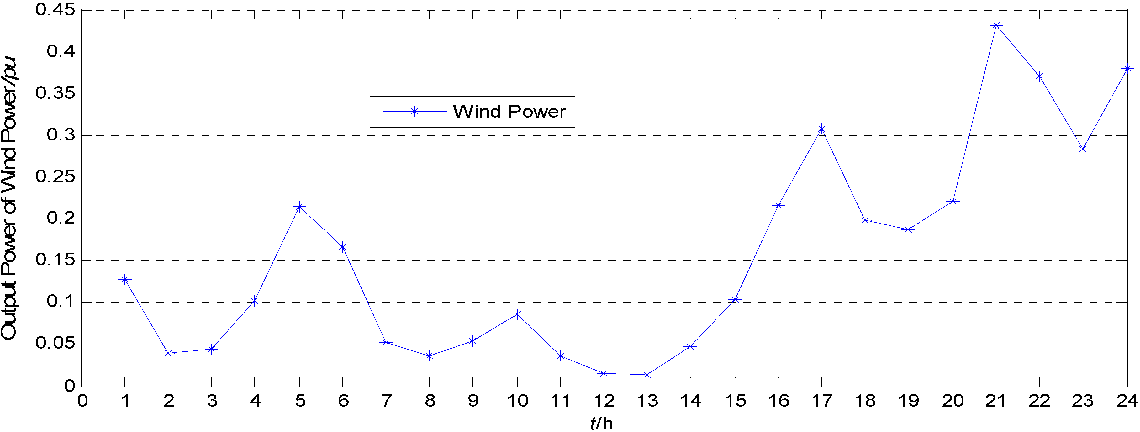
The predicted power output P_w of the wind farm in the 24 dispatch periods shown in Figure 5 is based on the wind speed–power function curve described in Equations (12) and (13), and the wind speed prediction in Figure 2. Table 5 compares the optimization results of the wind farm integrated into the system and the wind farm not integrated into the system power dispatch model. The energy-environmental efficiencies of the two models show no clear distinction due to low power output of the wind farm, whereas the operational cost experienced a decrease of $5,512.6268, from $99,721.9382 to $94,209.3114. Thus, the incorporation of wind power reduces primary energy cost, which proves to be a significant advantage of wind power.

Figure 5. Wind power forecast data for each time period.

Figure 5. Wind power forecast data for each time period.

Table 5. Comparison between optimization results of wind farmin and out the power system of low-carbon dispatch models.

Dispatch model	Operational cost/($)	Energy-environmental efficiency
Wind farm excluded	99,721.9382	10.9417
Wind farm included	94,209.3114	10.9301

Table 5. Comparison between optimization results of wind farmin and out the power system of low-carbon dispatch models.

Dispatch model	Operational cost/($)	Energy-environmental efficiency
Wind farm excluded	99,721.9382	10.9417
Wind farm included	94,209.3114	10.9301

Table 6 lists the comparison of computation times of multi-objective low-carbon dispatch and different single-objective dispatch models. As shown in Table 6, the calculation time consumed in solving multi-objective low-carbon dispatch model in a system consisting of six thermal power units and a grid-connected wind farm is 834.8493 s, which is longer than the time consumed in solving the single-objective dispatch model. Increased calculation time shows that the multi-objective model is more complicated and more difficult than the single-objective model. In the actual operation of the power system, the scheduling department generally makes power generation plan 24 h ahead of time. Therefore, the computing efficiency of the PSO-SA algorithm used in this paper to solve multi-objective low-carbon models can still meet the demand of the dispatch department to make daily generation plan. The PSO-SA algorithm used in this paper can act as a reasonable candidate for scheduling solution of the scheduling department of the power system.

Table 6. Comparison of calculation times of multi-objective and different single-objective dispatch models.

Dispatch model	Minimum operational cost	Optimum energy-environmental efficiency	Multi-objective low-carbon dispatch
CPU time/(s)	289.1735	349.4854	834.8493

Table 6. Comparison of calculation times of multi-objective and different single-objective dispatch models.

Dispatch model	Minimum operational cost	Optimum energy-environmental efficiency	Multi-objective low-carbon dispatch
CPU time/(s)	289.1735	349.4854	834.8493

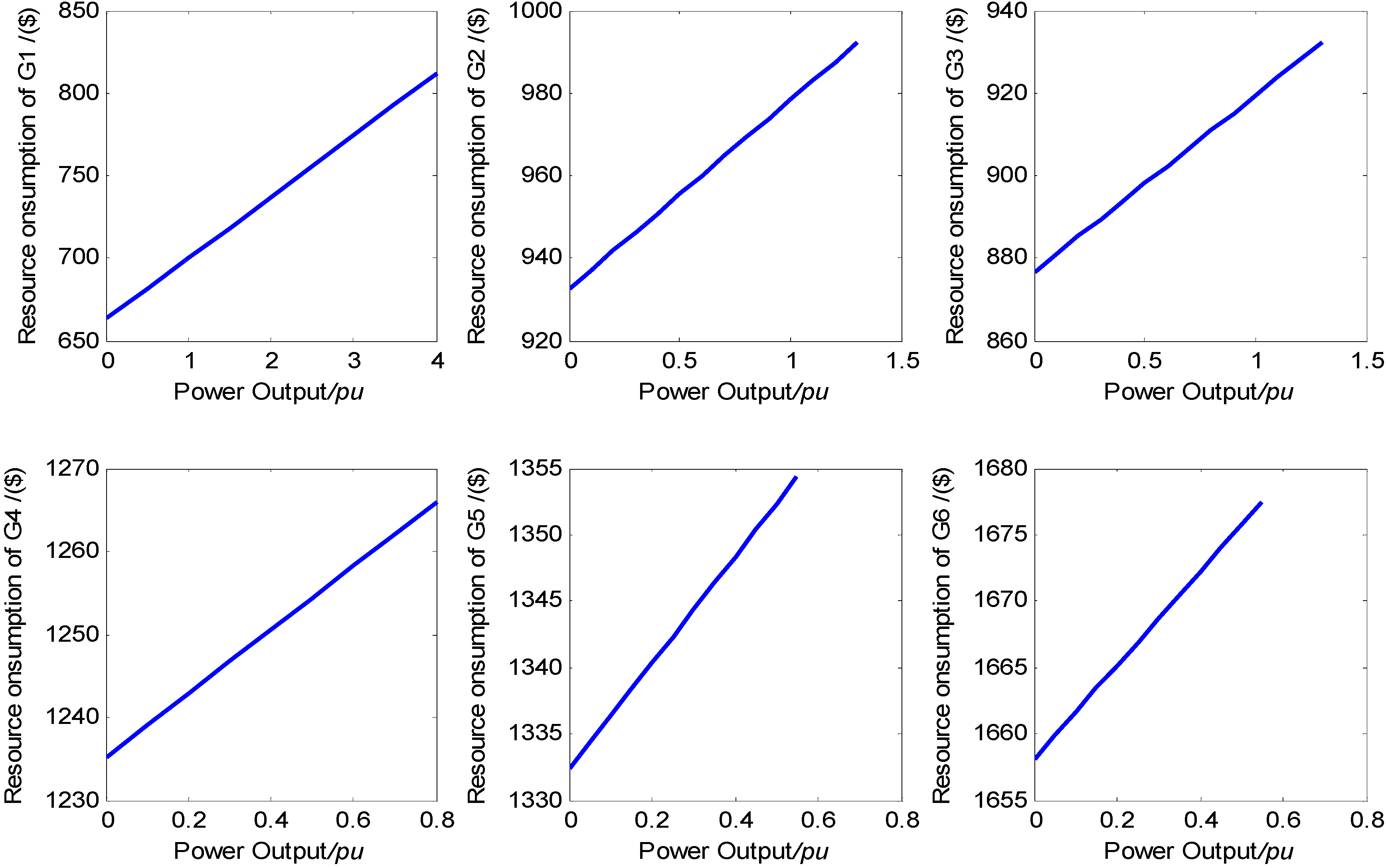
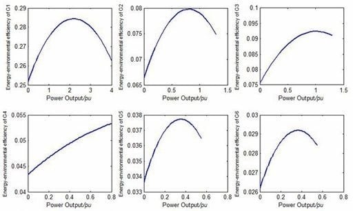
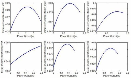
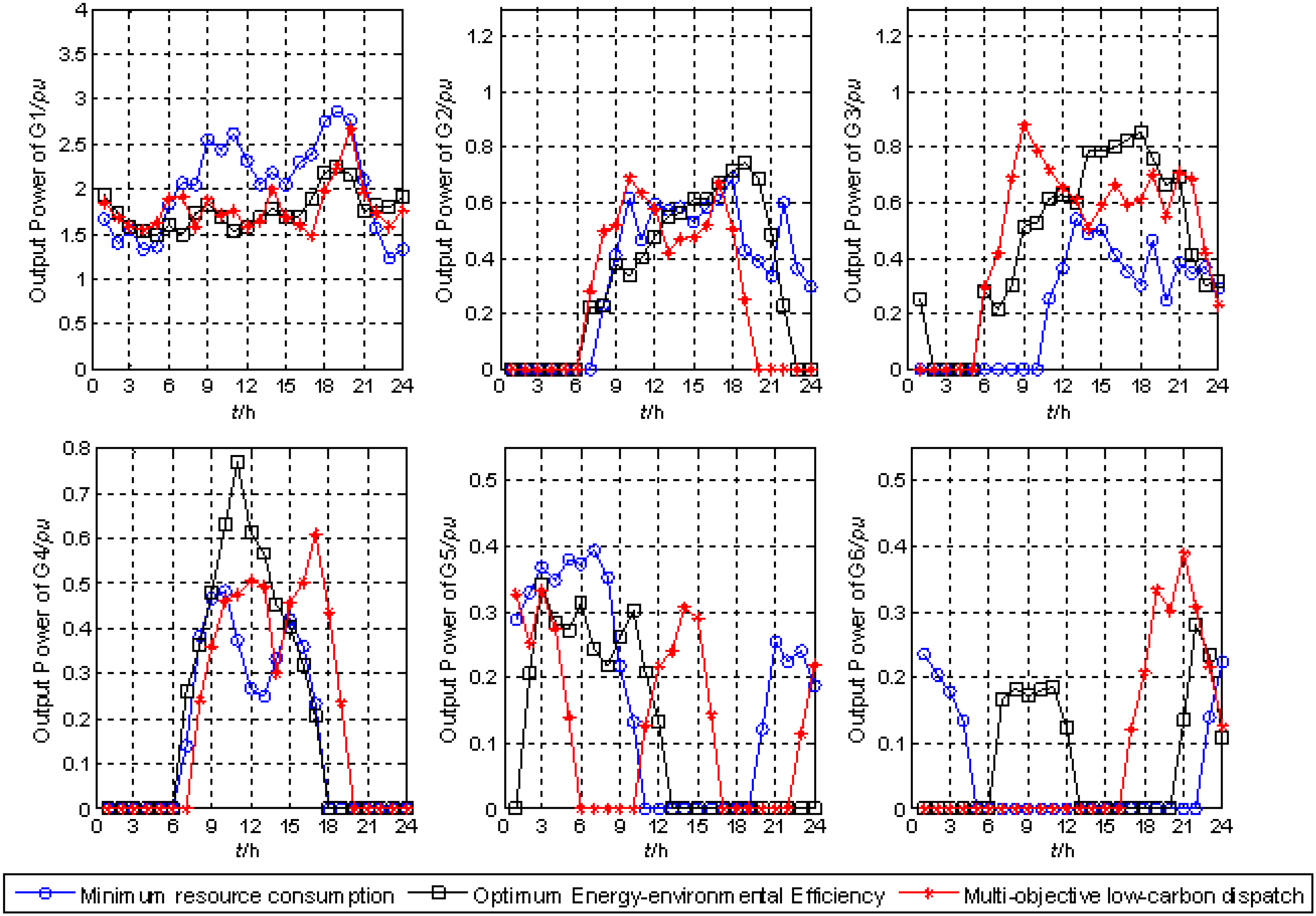
Table 7 compares the expected optimization objectives of the multi-objective low-carbon dispatch model with those of the single-objective dispatch models. Table 8 reveals the fuzzification result of the multi-objective dispatch model. Figure 6 shows the resource consumption-thermal power output curve. Figure 7 depicts the energy-environmental efficiency-thermal power output curve. Figure 8 renders the unit commitment and power output curves of the thermal generators, G₁ to G₆, of different dispatch models.

Table 7. Comparison of optimization results among multi-objective and different single-objective dispatch models.

Objective	Minimum operational cost	Optimum energy-environmental efficiency	Multi-objective low-carbon dispatch
Operational cost/($)	91,642.8250	97,312.1739	94,209.3114
Energy-environmental efficiency	10.5646	11.0364	10.9301

Table 7. Comparison of optimization results among multi-objective and different single-objective dispatch models.

Objective	Minimum operational cost	Optimum energy-environmental efficiency	Multi-objective low-carbon dispatch
Operational cost/($)	91,642.8250	97,312.1739	94,209.3114
Energy-environmental efficiency	10.5646	11.0364	10.9301

Table 7 and Table 8 show a maximum satisfaction value of 0.8122 when the multi-objective low-carbon dispatch optimization is performed, as shown in Table 8. Under this circumstance, generation operational cost is $94,209.3114, a $2,566.4864 (2.8%) increase compared with the operational cost of $91,642.8250 in the minimum operational cost dispatch and a $3,102.8625 (3.18%) reduction compared with the operational cost of $97,312.1739 in the optimum energy-environmental efficiency dispatch.

Table 8. Fuzzification result of multi-objective low-carbon dispatch model.

λ	μ(F)	μ(E)	F/($)	E
0.6373	0.9113	0.6373	92,432.7848	10.6894
0.6536	0.9026	0.6536	92,805.9495	10.7092
0.7138	0.8878	0.7138	93,109.7942	10.7752
0.7192	0.8825	0.7192	93,372.6540	10.7828
0.7513	0.8759	0.7513	93,605.9495	10.8252
0.7657	0.8562	0.7657	93,688.7945	10.8429
0.7741	0.8513	0.7741	93,935.8975	10.8763
0.7997	0.8489	0.7997	94,054.6232	10.8892
0.8050	0.8216	0.8050	94,117.0730	10.9102
0.8122	0.8158	0.8122	94,209.3114	10.9301

Table 8. Fuzzification result of multi-objective low-carbon dispatch model.

λ	μ(F)	μ(E)	F/($)	E
0.6373	0.9113	0.6373	92,432.7848	10.6894
0.6536	0.9026	0.6536	92,805.9495	10.7092
0.7138	0.8878	0.7138	93,109.7942	10.7752
0.7192	0.8825	0.7192	93,372.6540	10.7828
0.7513	0.8759	0.7513	93,605.9495	10.8252
0.7657	0.8562	0.7657	93,688.7945	10.8429
0.7741	0.8513	0.7741	93,935.8975	10.8763
0.7997	0.8489	0.7997	94,054.6232	10.8892
0.8050	0.8216	0.8050	94,117.0730	10.9102
0.8122	0.8158	0.8122	94,209.3114	10.9301

The corresponding energy-environmental efficiency value of the best compromise solution equals 10.9301, which is a 0.1063 (0.96%) decrease from 11.0364 of the optimum energy-environmental efficiency dispatch and a 0.3655 (3.46%) increase from 10.5646 of the minimum operational cost dispatch. According to Table 7, optimization of the multi-objective low-carbon dispatch model bears higher total generation operational cost than that of the optimization of minimum operational cost dispatch model and better energy-environmental efficiency than that of the optimization of the optimum energy-environmental efficiency dispatch model. The multi-objective model accounts for both economy and ecology in power generation, whereas the pre-mentioned single-objective models emphasize only a certain side. Based on the above comparative analysis, the multi-objective dispatch model proposed in the present paper outperforms the single-objective ones when the two conflicting optimization objectives are both considered. The proposed model strikes a balance between the two and precisely reflects the operating condition of the thermal generators while optimizing the wind power output dispatch. These characteristics distinguish the proposed model from the traditional single-objective ones.

Table 8 indicates that operational cost increases along with the enhancement of fuzzy satisfaction, whereas the energy-environmental efficiency increases greatly. Nevertheless, control of CO₂ emission is bound to raise generation costs. This finding further proves the necessity and efficiency of the proposed model in improving energy-environmental efficiency and cutting down carbon emission. The decision maker can choose a compromise solution subjectively to meet different power market requirements based on the optimization result.

Figure 6. Curves of resource consumption values of unit G1 to G6.

Figure 6. Curves of resource consumption values of unit G1 to G6.

Figure 6 shows that the resource consumption values of the six generators increase monotonously with the escalation of power output level. The operational cost of thermal unit is determined by resource consumption. This characteristic leads to the active power of all thermal generator units in different dispatching periods close to the relevant power output value of the minor resource consumption when using the objective function of minimum operational cost in optimal dispatching. Besides, those with minor resource consumption in the same load distribution have the priority to take the load. Nevertheless, the energy-environmental efficiency curve and the resource consumption curve show different characteristics.

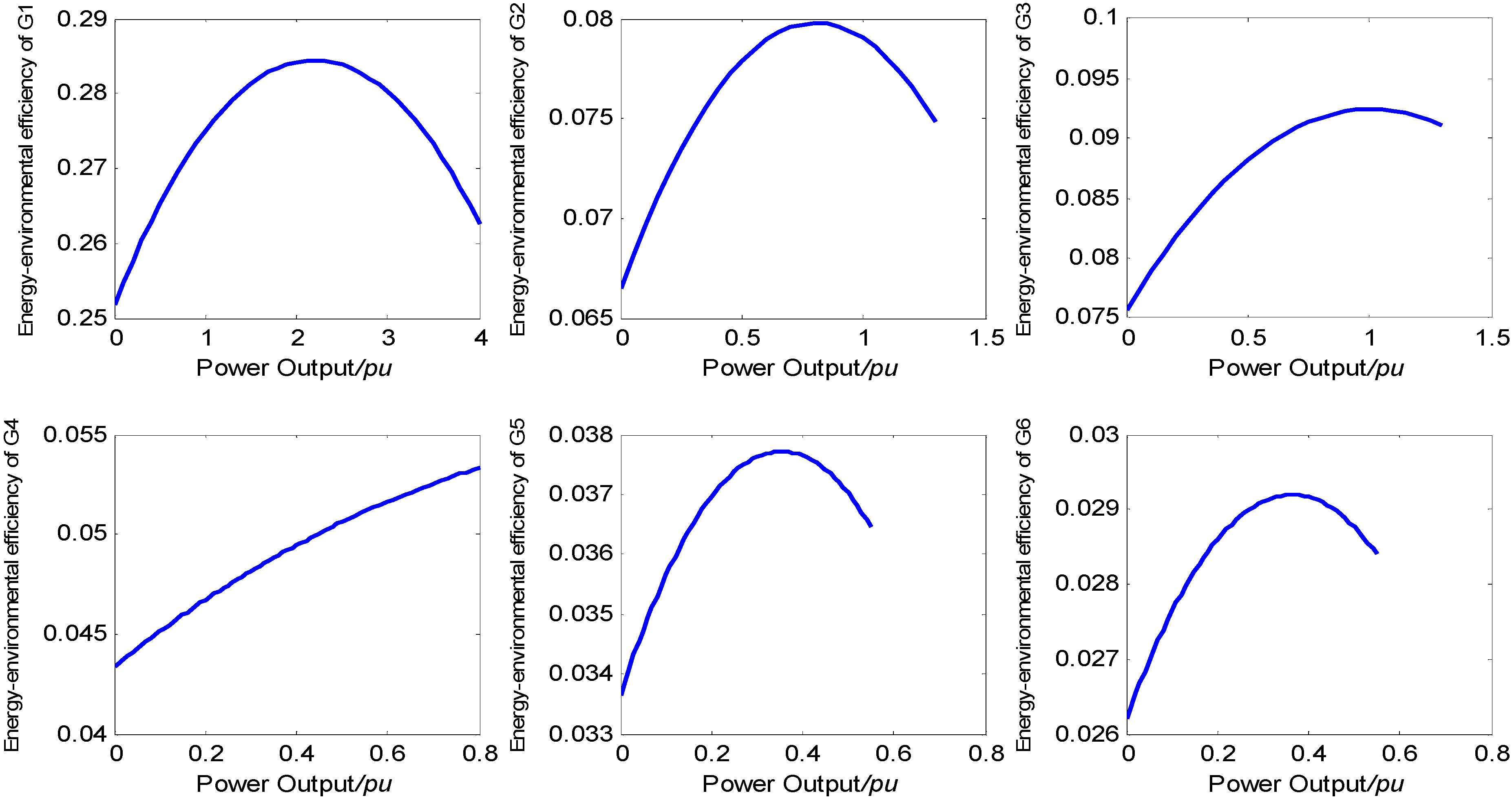
Figure 7 shows the energy-environmental efficiency values of the six generators under different power output levels. The energy-environmental efficiency of the thermal generators does not monotonically increase along with the escalation of the power output, except in the fourth unit. They generally have parabolic curves that make energy-environmental efficiency values lower on both light and heavy power output levels. This characteristic significantly influences the load dispatch strategy when considering energy-environmental efficiency. For a certain generator, power output in different dispatch periods converges to the point where the energy-environmental efficiency reaches its optimum value. For generators with the same power output character, those with better energy-environmental efficiency have the priority to take the load.

Figure 7. Curves of energy-environmental efficiency values of unit G1 to G6.

Figure 7. Curves of energy-environmental efficiency values of unit G1 to G6.

The abovementioned issue may be proven by the power output curves in Figure 8. In either single-objective model with optimal energy-environmental efficiency or multi-objective low-carbon dispatch model to carry out the dispatch, the power output of the thermal generators fluctuates around the point of the best energy-environmental efficiency in most dispatch intervals. When the load is relatively low, units with worse energy-environmental efficiency will be cut off. This way, the overall energy-environmental efficiency is improved because the units with better energy-environmental efficiency are ensured to operate around their optimum operation point. When the minimum operational cost model is adopted, the power output of G₁ to G₆ are reduced for cost control, resulting in a relatively low energy-environmental efficiency value. Under this circumstance, operational cost is lessened at the expense of environmental damage, contrary to the low-carbon developing policy. For generators of the same power output characteristic, the ones with better energy-environmental efficiency will take on the load first. For example, if G₂ and G₃ have the same power output character, as shown in Figure 7, then G₃ exceeds G₂ in operating time and power output when energy-environmental efficiency is considered. A similar analysis applies to G₅ and G₆ with an identical conclusion.

The energy-environmental efficiency curve of G₄ monotonically increases with the growth of its power output. A comparison of the power output curves of G₄ in the three different dispatch models suggests that G₄ offers the largest power output in the optimum energy-environmental efficiency model. In the multi-objective model, the power output of G₄ falls to some extent, but still outweighs the power output in the minimum operational cost model significantly. Therefore, the above comparative analysis reveals that the unit commitment strategy and load dispatch scheme change greatly when energy-environmental efficiency is considered. Units with better energy-environmental efficiency gain the priority to be loaded to augment the operational cost of power generation. When the multi-objective low-carbon dispatch model is introduced, reasonable operational cost is achieved while energy-environmental efficiency is improved and low-carbon dispatch is promoted.

Figure 8. Curves of daily output of units G1 to G6 with different objectives.

Figure 8. Curves of daily output of units G1 to G6 with different objectives.

Figure 8 shows that in the optimization of the minimum operational cost model, units with lower operational cost possess absolute advantage in price regardless of the energy-environmental efficiency. Thus, these units hold loading priority. When energy-environmental efficiency serves as the optimization objective, units with better energy-environmental efficiency have superiority over other generators, irrespective of operational cost. Thus, such units hold loading priority. When both economic and environmental indexes are considered, optimization of the multi-objective model involves the impartiality for power generators and brings forward the spirit of low-carbon power dispatch.

Energy-environmental efficiency cannot be measured by money like the operational cost of traditional generators. Rather, it appears as a kind of invisible capital. Overall, by taking energy-environmental efficiency into account, the operational cost of thermal generators slightly increases, whereas the energy-environmental efficiency of the power generation system escalates unconsciously, leaving the ecology less polluted. Therefore, incorporation of the energy-environmental efficiency into the power dispatch model bears profound meanings in the background of global promotion of green energy development and low-carbon economy. Low-carbon dispatch possesses expansive potential applications in appliances.

7. Conclusions

This paper introduces wind speed prediction technique and energy-environmental efficiency concept into the optimization dispatch problem of a wind-incorporated power system. The time series method is adopted to perform short-term wind speed prediction and offer relatively accurate power output data for dispatch departments to mitigate the impact of wind speed fluctuation on the power system dispatch and its operation. Low-carbonization is stressed by the introduction of energy- environmental efficiency in the modeling process, resulting in a multi-objective power dispatch model that pursues both minimum operational cost and optimal energy-environmental efficiency. The proposed model is built from the ecological perspective, emphasizing the effect of power generation on the environment. The model positively affects the present power system dispatch technique in the strategic policy of large-scale wind power promotion and green low-carbon development. Multi-objective fuzzy optimization and PSO-SA algorithms are adopted to solve the low-carbon dispatch model and increase its calculation precision. Simulation results prove the reasonability of the proposed multi-objective low-carbon dispatch model. The consequent dispatch strategy offers reference to traditional power generation dispatch. Energy-environmental efficiency should be a key factor in power system dispatch and operation.

The following conclusions are also reached: (1) Wind speed prediction is critical in the optimization of the dispatch of wind-incorporated power systems. Progress in prediction techniques is beneficial to the overall security and stability of power system dispatch and operation; (2) With environmental protection becoming the societal focus, more strict limits on pollutant emission are set. The energy-environmental efficiency index effectively evaluates the transformation efficiency and environmental effect of different primary energies, objectively reflecting the effect of power generation on the ecology; (3) Traditional single-objective dispatch models are not adequate for dealing with wind-incorporated power system dispatch problems. In contrast, the multi-objective low-carbon dispatch model considering both minimum operational cost and optimum energy-environmental efficiency is a more practical method.

Finally, it should be pointed out that this paper has validated the rationality of the proposed multi-objective low-carbon dispatch model under the simulation of the system containing six thermal power units and a grid-connected wind farm. The optimization result can be used as a reference for existing power system dispatch. However, further research and consummation are needed to determine whether multi-objective low-carbon dispatch model and PSO-SA algorithm can implement the time scales required for scheduling dispatch over real systems (on the order of thousands of generators).

References

1. 120 Gigawatt of Wind Turbines Globally Contribute to Secure Electricity Generation; World Wind Energy Association: Bonn, Germany; Available online: http://www.wwindea.org/home/index2.php?option=com_content&do_pdf=1&id=223 (accessed on 25 November 2010).
2. Ren, B.Q.; Jiang, C.W. A review on the economic dispatch and risk management considering wind power in the power market. Renew. Sustain. Energy Rev. 2009, 13, 2169–2174. [Google Scholar] [CrossRef]
3. 2010 Chinese Wind Power Capacity Statistics; Chinese Wind Energy Association: Beijing, China; Available online: http://www.cwea.org.cn/download/display_info.asp?id=39 (accessed on 17 August 2011).
4. Chen, C.L.; Lee, T.Y.; Jan, R.M. Optimal wind-thermal coordination dispatch in isolated power systems with large integration of wind capacity. Energy Convers. Manag. 2006, 47, 18–19. [Google Scholar]
5. Miranda, V.; Hang, P.S. Economic dispatch model with fuzzy wind constraints and attitudes of dispatchers. IEEE Trans. Power Syst. 2005, 20, 2143–2145. [Google Scholar] [CrossRef]
6. Hetzer, J.; Yu, D.C.; Bhattarai, K. An economic dispatch model incorporating wind power. IEEE Trans. Energy Convers. 2008, 23, 603–611. [Google Scholar] [CrossRef]
7. Liu, X.; Xu, W. Minimum emission dispatch constrained by stochastic wind power availability and cost. IEEE Trans. Power Syst. 2010, 25, 1705–1713. [Google Scholar] [CrossRef]
8. Foley, A.M.; Murguvlia, A.; Leahy, P.G.; McKeogh, E.J. Current methods and advances in forecasting of wind power generation. Renew. Energy 2012, 37, 1–8. [Google Scholar] [CrossRef] [Green Version]
9. Pourmousavi, S.A.; Ardehali, M.M. Very short-term wind speed prediction: A new artificial neural network-markov chain model. Energy Convers. Manag. 2011, 52, 738–745. [Google Scholar] [CrossRef]
10. Ackermann, T. Wind Power in Power System; John Wiley & Sons: London, UK, 2005. [Google Scholar]
11. Chen, Q.X.; Kang, C.Q.; Xia, Q. Modeling flexible operation mechanism of CO2 capture power plant and its effects on power-system operation. IEEE Trans. Energy Convers. 2010, 25, 853–861. [Google Scholar] [CrossRef]
12. Maria, M.B.; Pardo, A. What you should know about carbon markets. Energies 2008, 1, 120–153. [Google Scholar] [CrossRef] [Green Version]
13. Carrion, M.; Arroyo, J.M. A computationally efficient mixed-integer linear formulation for the thermal unit commitment problem. IEEE Trans. Power Syst. 2006, 21, 1371–1378. [Google Scholar] [CrossRef]
14. Han, X.S.; Gooi, H.B.; Kirschen, D.S. Dynamic economic dispatch: Feasible and optimal solutions. IEEE Trans. Power Syst. 2001, 16, 22–28. [Google Scholar] [CrossRef]
15. Chaturvedi, K.T.; Manjaree, P.; Laxmi, S. Self-organizing hierarchical particle swarm optimization for nonconvex economic dispatch. IEEE Trans. Power Syst. 2008, 23, 1079–1087. [Google Scholar] [CrossRef]
16. Liu, D.R.; Cai, Y. Taguchi method for solving the economic dispatch problem with nonsmooth cost functions. IEEE Trans. Power Syst. 2005, 20, 2006–2014. [Google Scholar] [CrossRef]
17. Lu, Y.L.; Zhou, J.Z.; Qin, H.; Wang, Y.; Zhang, Y.C. Environmental/Economic dispatch problem of power system by using an enhanced multi-objective differential evolution algorithm. Energy Convers. Manag. 2011, 52, 1175–1183. [Google Scholar] [CrossRef]
18. Abido, M.A. A niched pareto genetic algorithm for multiobjective environmental/economic dispatch. Int. J. Electr. Power Energy Syst. 2003, 25, 97–105. [Google Scholar] [CrossRef]
19. Abido, M.A. Multiobjective particle swarm optimization for environmental/economic dispatch problem. Electr. Power Syst. Res. 2009, 79, 1105–1113. [Google Scholar] [CrossRef]
20. Talaq, J.H.; El-Hawary, F.; EI-Hawary, M.E. Summary of environmental/economic dispatch algorithms. IEEE Trans. Power Syst. 1994, 9, 1508–1516. [Google Scholar] [CrossRef]
21. King, T.D.; EI-Hawary, M.E.; EI-Hawary, F. Optimal environmental dispatching of electric power systems via an improved Hopfield neural network model. IEEE Trans. Power Syst. 1995, 10, 1559–1565. [Google Scholar] [CrossRef]
22. Cai, J.J.; Ma, X.Q.; Li, Q.; Li, L.X.; Peng, H.P. A multi-objective chaotic particle swarm optimization for environmental/economic dispatch. Energy Convers. Manag. 2009, 50, 1318–1325. [Google Scholar] [CrossRef]
23. Chena, S.D.; Chen, J.F. A direct Newton-Raphson economic emission dispatch. Int. J. Electr. Power Energy Syst. 2003, 25, 411–417. [Google Scholar] [CrossRef]
24. Cheng, C.K. Wind energy dispatch considering environmental and economic factors. Renew. Energy 2010, 35, 2217–2227. [Google Scholar] [CrossRef]
25. Ummels, B.C.; Gibescu, M.; Pelgrum, E.; Kling, W.L.; Brand, A.J. Impacts of wind power on thermal generation unit commitment and dispatch. IEEE Trans. Energy Convers. 2007, 22, 44–51. [Google Scholar] [CrossRef]
26. Boehme, T.; Wallace, A.R.; Harrison, G.P. Applying time series to power flow analysis in networks with high wind penetration. IEEE Trans. Power Syst. 2007, 22, 951–957. [Google Scholar] [CrossRef]
27. Sfetsos, A. A comparison of various forecasting techniques applied to mean hourly wind speed time series. Renew. Energy 2000, 21, 23–35. [Google Scholar] [CrossRef]
28. Pashardes, S.; Christofides, C. Statistical analysis of wind speed and direction in Cyprus. Sol. Energy 1995, 55, 405–414. [Google Scholar] [CrossRef]
29. Wind Turbine Control Methods; National Instruments Corporation: Austin, TX, USA; Available online: http://zone.ni.com/devzone/cda/tut/p/id/8189 (accessed on 7 October 2010).
30. Cardu, M.; Baica, M. Regarding a global methodology to estimate the energy-ecologic efficiency of thermopower plants. Energy Convers. Manag. 1999, 40, 71–87. [Google Scholar] [CrossRef]
31. Cardu, M.; Baica, M. Regarding a new variant methodology to estimate globally the ecologic impact of thermopower plants. Energy Convers. Manag. 1999, 40, 1569–1575. [Google Scholar] [CrossRef]
32. Cardu, M.; Baica, M. Regarding the energy ecologic efficiency of desulphurization and denox systems and installations in thermopower plants. Energy Convers. Manag. 2000, 41, 1155–1164. [Google Scholar] [CrossRef]
33. Kennedy, J.; Eberhart, R. Particle swarm optimization. In Proceedings of the 1995 IEEE International Conference on Neural Networks, Perth, Australia, 27 November–1 December 1995; pp. 1942–1948.
34. Kirkpatrick, S.; Gelatt, C.D.; Vecchi, M.P. Optimization by simulated annealing. Science 1983, 220, 671–680. [Google Scholar] [CrossRef] [PubMed]
35. Fu, A.L.; Lei, X.J.; Xiao, X. The aircraft departure scheduling based on particle swarm optimization combined with simulated annealing algorithm. In Proceedings of the 2008 IEEE Congress on Evolutionary Computation, Hong Kong, China, 1–6 June 2008; pp. 1393–1398.
36. Sadati, N.; Amraee, T.; Ranjbar, A.M. A global particle swarm-based-simulated annealing optimization technique for under-voltage load shedding problem. Appl. Soft Comput. 2009, 9, 652–657. [Google Scholar] [CrossRef]
37. Li, J.B.; Liu, X.G. Melt index prediction by RBF neural network optimized with an MPSO-SA hybrid algorithm. Neurocomputing 2011, 74, 735–740. [Google Scholar] [CrossRef]
38. Wang, Z.S.; Li, L.C.; Li, B. Based on particle swarm optimization and simulated annealing combined algorithm for reactive power optimization. In Proceedings of the 2009 Asia-Pacific Power and Energy Engineering Conference, Wuhan, China, 28–30 March 2009; pp. 1909–1913.
39. Ajami, A.L.; Aghajani, G.H.; Pourmahmood, M. Optimal location of FACTS devices using adaptive particle swarm optimization hybrid with simulated annealing. J. Electr. Eng. Technol. 2010, 5, 179–190. [Google Scholar] [CrossRef]
40. Cui, Y.B. Application of simulated annealing particle swarm optimization algorithm in power coal blending optimization. In Proceedings of the 2008 International Conference on Wireless Communication, Networking and Mobile Computing, Dalian, China, 12–14 October 2008; pp. 1–4.
41. Zangeneh, A.; Jadid, S. Fuzzy multiobjective model for distributed generation expansion planning in uncertain environment. Eur. Trans. Electr. Power 2011, 21, 129–141. [Google Scholar] [CrossRef]
42. Huang, C.M.; Yang, H.T.; Huang, C.L. Bi-objective power dispatch using fuzzy satisfaction-maximizing decision approach. IEEE Trans. Power Syst. 1997, 12, 1715–1721. [Google Scholar] [CrossRef]