Numerical Modelling of Mutual Effect among Nearby Needles in a Multi-Needle Configuration of an Atmospheric Air Dielectric Barrier Discharge

Abstract

A numerical study has been conducted to understand the mutual effect among nearby needles in a multi-needle electrode dielectric barrier discharge. In the present paper, a fluid-hydrodynamic model is adopted. In this model, the mutual effect among nearby needles in a multi-needle configuration of an atmospheric air dielectric barrier discharge are investigated using a fluid-hydrodynamic model including the continuity equations for electrons and positive and negative ions coupled with Poisson’s equation. The electric fields at the streamer head of the middle needle (MN) and the side needles (SNs) in a three-needle model decreased under the influence of the mutual effects of nearby needles compared with that in the single-needle model. In addition, from the same comparison, the average propagation velocities of the streamers from MN and SNs, the electron average energy profile of MN and SNs (including those in the streamer channel, at the streamer head, and in the unbridged gap), and the electron densities at the streamer head of the MN and SNs also decreased. The results obtained in the current paper agreed well with the experimental and simulation results in the literature.

1. Introduction

Non-thermal plasma (NTP) produced through dielectric barrier discharges (DBDs) has a number of useful industrial applications, such as surface modification, environmental protection, medicine, and plasma displays, because DBDs can produce large volume and high-energy-density NTPs at atmospheric pressure over a wide range of frequencies without employing expensive vacuum equipment [1,2,3,4,5,6].

Research on DBDs mainly focuses on two topics: application technologies and the physical mechanism of the discharges [1]. The first, which study the actual application of DBDs, are primarily implemented through experimental observation [3,5,7,8,9] and theoretical analysis [5,10,11]. They mainly aim at improving the plasma-treatment efficiency and reducing energy consumption. Generally, plane-to-plane or coaxial structures are adopted for DBD electrodes [1]. To increase the energy-input efficiency, improvements for the two structures have been proposed, such as multineedle-to-plane (MP) [5,7,10], mesh-to-plate [3,8], trench-to-plane [12,13], and multineedle-to-cylinder (MC) configurations [9,11]. These configurations have been proven better for some applications because they can generate non-uniform electric fields in space, resulting in low operating voltage and low dielectric loss, which are beneficial for commercial applications. For example, Takaki [12,14,15] reported that the NO_x removal efficiency through an MP reactor was higher than that through the plane-to-plane reactor. Our previous study showed that the MC configuration reduced the initial discharge and operating voltages as well as improved the transported charges compared with the coaxial configuration, both at 50 Hz and at higher frequencies (17–29 kHz) [9,16]. Meanwhile, a quasi-static field simulation based on three-dimensional (3-D) finite-element method (FEM) was employed to investigate the DBD characteristics of MC configurations, which was experimentally confirmed in [11].

On the other hand, research on the physical mechanism of the discharge of DBD concentrates on the definition of discharge properties (filament discharge [17], Townsend glow discharge [18], and glow discharge [1,19,20,21]) and local discharge characteristics [22]. Considering the complexity of the plasma processes created by DBDs, mathematical modelling and numerical simulations are essential tools used to increase our fundamental understanding of the subject [23,24,25,26,27]. Research on local discharge characteristics mainly focuses on the space-time evolution of particles (e.g., excitation and ionization by an electron of a neutral particle, recombination of electrons and ions, and electron thermal and non-thermal attachment and detachment processes), electron mean energy profile, and photo-ionization [28]. This research cannot be easily realized through experimental observation but must be conducted via theoretical analysis. With the advent of more powerful computers and more sophisticated algorithms, numerical modelling has been increasingly employed and will continue to benefit the investigation of non-equilibrium plasma caused by gas discharge [23,24,25,26,28,29].

At the high pressures usually encountered in DBD, streamer discharge takes place because of the considerable space charge generated during the first avalanche transit through the gap [23]. The streamer mechanism was initially proposed by Raether [30] and Loeb and Meek [31] to explain the electrical breakdown of overvolted gaps at near-atmospheric pressure. In investigating the local mechanism of streamer discharge, the streamer discharge can be approximately regarded as a low-temperature and non-equilibrium plasma. At present, three basic models are employed in describing the evolution of charged particles in non-equilibrium plasma [23,24,25,26,27,28,29,32,33,34,35,36,37,38,39,40,41,42,43]: the fluid-hydrodynamic, particle-in-cell/Monte Carlo collision (PIC/MCC), and hybrid models. Impressive advances have been achieved in the development of these models, and they have been widely employed in both the investigation of fundamental physics and in the design of plasma equipment. Each method has its advantages and disadvantages. The fluid-hydrodynamic models are widely used and can be applied to analyze polyatomic and monatomic gas discharges without pressure limitations [38]. Natalia et al. reported a multifluid hydrodynamic simulation that investigated the ion energy and angular distributions incident on dielectric flat surfaces resulting from the intersection of DBD filaments subjected to atmospheric-air pressure [24]. The PIC/MCC method provides the most detailed information on the properties (e.g., velocity distributions) of electrons, ions, and atoms in non-equilibrium plasma [41,43]. Hybrid models have been developed to implement practical simulations without losing the non-equilibrium properties, such as ionization and dissociation rates. Kushner [27] proposed a hybrid model to address different physical processes or the same physical processes using different techniques. The hybrid model in [29,34] combined the computational modules, including sheath, magnetostatic, electromagnetic, electron energy-transport, fluid kinetics–Poisson, surface kinetic, dust-transport, radiation-transport Monte Carlo, plasma-chemistry Monte Carlo, real-time-control, sputter module, and ion Monte Carlo simulation and circuit modules. These modules transfer information among themselves in hierarchical manner; thus, algorithms best suited for the conditions of interest can be used without affecting the other modules. Meanwhile, Célestin et al., have made great progress in simulating streamer propagation in point-to-plane and point-to-point geometries using ghost fluid method combined with the finite volume approach [44,45,46]. Although the PIC/MCC model provides a clear physical picture of the avalanche-to-streamer transition and its subsequent propagation, vast majority of numerical simulations for such phenomena employed the hydrodynamic diffusion-drift approximation models to describe the evolution of charge densities because kinetic simulations are extremely time consuming [23,34]. In addition, the amount of calculation required for the hybrid kinetic-fluid model is so enormous that multicore processors and parallel computers are required [23,29]. This model could be one of the main models to be adopted for the investigation of DBD in the future. Therefore, the current paper, which addresses the mutual effect among nearby needles in atmospheric-air DBD, mainly uses the simplified fluid-hydrodynamic model that contains continuity equations for electrons, ions, and neutral particles coupled with the Poisson's equation for a local field [47,48].

In our previous research, the mutual effect of nearby needles was found to influence the DBD characteristics in multi-needle configuration [11]. This effect appeared to be stronger when nearby sets of needles were arranged parallel, i.e., inter axial needle rotation angle was set to be 0°. Rong et al., also observed the mutual effect among nearby needles in MP configuration, which was experimentally validated [5]. Considering that the quasi-static field simulation [11] and the static field simulation [5] were adopted and the process of avalanche formation was the main aim of these works, the mutual effect mechanism in streamer discharge of the multi-needle geometry was not clear. Therefore, the hydrodynamic model is adopted in the current paper to investigate numerically the space-time evolutions of electric fields, particles (electron and positive ions), and electron average energy profile of the multi-needle configuration in atmospheric air and to reveal further the mutual effect among nearby needles.

2. Simulation Model

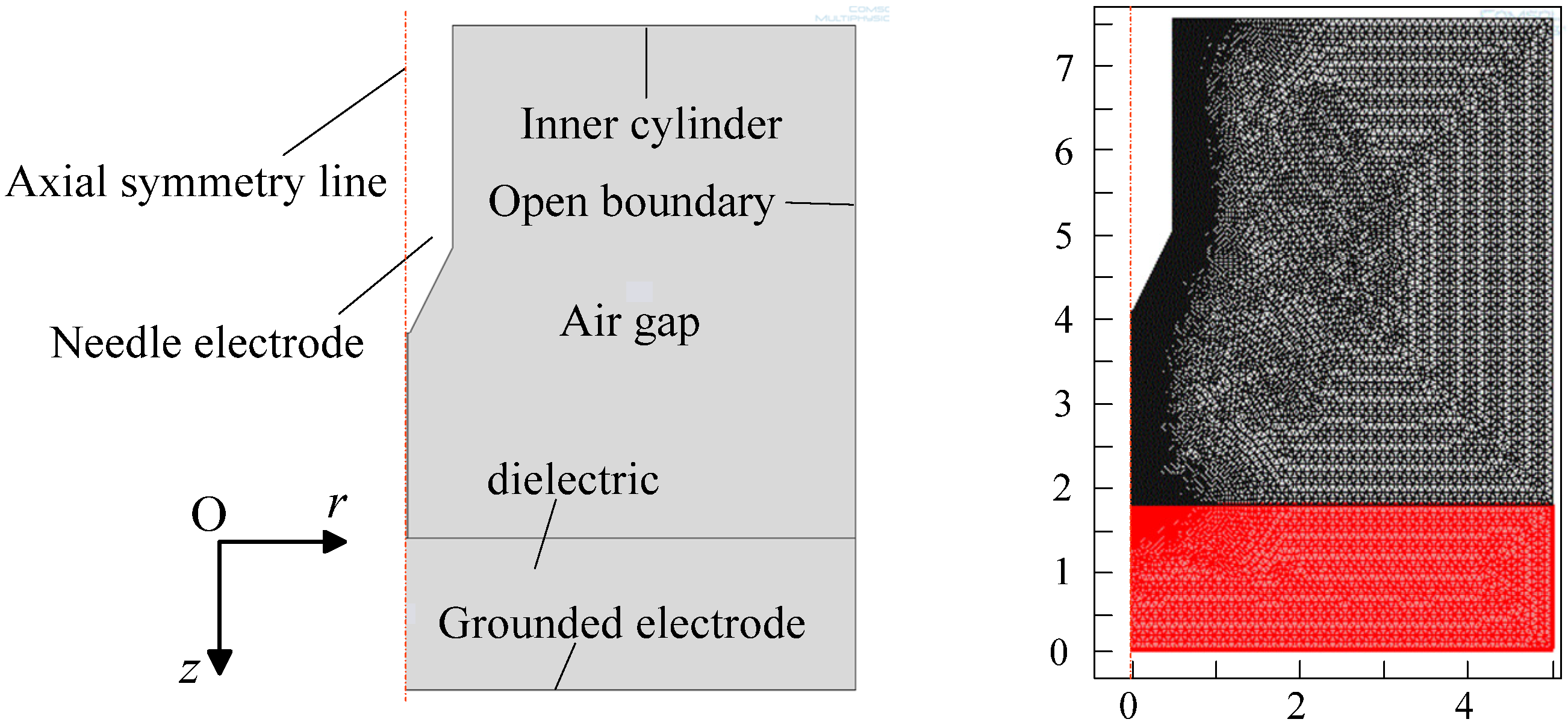
2.1. Geometry Models in the Simulation

The multi-needle geometry model used in the current simulation, a simplified two-dimensional (2-D) axisymmetric model patterned after the 3-D model in [11], is shown in Figure 1(a). In our previous study, the mutual effect among nearby needles was found to influence the DBD characteristics in multi-needle configuration [11], and the effect is stronger when the adjacent sets of needles are arranged parallel. The 3-D geometry is shown in Figure 2, in which the multineedle electrode is composed of three sets of needles arrayed on a 5 mm diameter copper rod. However, the simulation of the 3-D geometry was time-consuming and limited by the computer employed. Therefore, the X–Z cross section in the 3-D geometry was adopted as the 2-D simplified axisymmetric model [Figure 1(a)]. The simplified simulation model in Figure 1(a) is not completely equivalent to the 3-D geometry in Figure 2. Considering that the present study is mainly aimed at the mutual effect among nearby needles, and the effect on the cross section in the 2-D axisymmetric model is analogous to those in the 3-D model to a certain extent, the simplified 2-D axisymmetric model is a reasonable, acceptable, and a time-saving option. In the current paper, the needle length is 3.5 mm and the distance among nearby needles is equal to 5 mm. The diameter and the tip angle of the needles are 1 mm and 53°, respectively. The gap length between the needle tips and the dielectric surface is 2.25 mm.

Figure 1. Geometry model in simulation and the model of the needle tip (units in milimeters). (a) Geometry model used in simulation; (b) Schematic diagram of the needle tip (units in millimeters).

Figure 1. Geometry model in simulation and the model of the needle tip (units in milimeters). (a) Geometry model used in simulation; (b) Schematic diagram of the needle tip (units in millimeters).

Streamer discharge has been proven to occur near the streamer head and propagate along the axial direction in multi-needle DBD. Thus, due to high electric field and charge densities, a very fine “unstructured mesh” must be used around the needle tip, along the axial symmetry line, and along the line from the needle tip perpendicular to the dielectric layer (Figure 3). The mesh parameters are shown in Table 1. Usually, the tip of the needle projection works as a singular point, indicating the presence of an infinite electric field near the tip. Furthermore, the simulation result was significantly sensitive to the mesh resolution in this region [49]. Therefore, the needle tip is treated as shown in Figure 1(b) during the modelling, as demonstrated in [11].

Figure 2. 3-D geometry in the current work (the cross section in the dashed frame is adopted as the simplified 2-D simulation model).

Figure 2. 3-D geometry in the current work (the cross section in the dashed frame is adopted as the simplified 2-D simulation model).

Figure 3. Computational domain of 2-D model in an unstructured triangular grid (units in millimeters).

Figure 3. Computational domain of 2-D model in an unstructured triangular grid (units in millimeters).

Table 1. Mesh statistics.

Mesh parameter	Results
Triangular elements	113,554
Edge elements	2,755
Minimum element quality	0.6566
Average element quality	0.9635
Element area ratio	4.298 × 10−11
Mesh area	7.0 × 10−5 m2

Table 1. Mesh statistics.

Mesh parameter	Results
Triangular elements	113,554
Edge elements	2,755
Minimum element quality	0.6566
Average element quality	0.9635
Element area ratio	4.298 × 10−11
Mesh area	7.0 × 10−5 m2

Furthermore, the half-needle geometry model (Figure 4) was also adopted and researched to compare the simulation results of the three-needle (TNG) and single-needle geometries (SNG) and to analyze the mutual effect of nearby needles.

The models employed in this work were built in (2-D) axial symmetry configurations and implemented in COMSOL Multiphysics^® package based on FEM [49], in which a time-dependent solver PARDISO was used. Automatic geometry shape order was chosen as the basis functions with triangular-shaped elements. Time resolution adopted was backward differentiation formula (BDF).

All the calculations were conducted using one machine with two 3.4 GHz Intel(R) I7-2600 processors parallel running in 64-bit mode, 16 GB memory, and Windows 7 operating system.

Figure 4. The geometry model including a half needle (units in millimeters).

Figure 4. The geometry model including a half needle (units in millimeters).

2.2. Mathematical Model

A considerable amount of theoretical, numerical, and experimental efforts have been devoted to understanding the development of an electron avalanche, its transition into streamers, propagation of the streamer fronts [23,50,51,52], and formation of a glow. These factors constitute the main mechanisms of non-thermal gas discharge plasma production under atmospheric pressure. In the current work, primary streamer propagation is mainly aimed at.

The continuity equations for electrons, positive ions, and negative ions (to account for the development of the space-charge) has been proven to be the simplest set of equations within the fluid model framework that contains the basic physics necessary for gaseous discharges. This set of equations is coupled with the Poisson’s equation (to account for the modification of the electric field due to space-charge) [23]. The continuity equations in their multidimensional form are as follows [52,53]:

(1)

(2)

(3)

where S is the source term due to photoionization, t is the time; subscripts e, p, and n represent the electrons, positive ions, and negative ions respectively; N_e, N_p, and N_n are the ion number densities; ${\overrightarrow{W}}_e$, ${\overrightarrow{W}}_p$, and ${\overrightarrow{W}}_n$ represent the electron, positive ion, and negative ion drift velocities, respectively; and D_e is the electron diffusion coefficient. The symbols α, η, β_ep, and β_np denote the ionization, attachment, electron–positive-ion recombination and negative-ion–positive-ion recombination coefficients, respectively. The recombination coefficients β_ep and β_np are considered constant and equal to β, following Morrow and Lowke [42]. The transport properties, which are functions of the local electric field, are given in Table 2.

Table 2. Transport properties of air given by Morrow and Lowke [42] and Kang et al. [17] (E in volts per centimeter).

Properties	Functions
α (cm−1)	3500exp(−1.65 × 105E−1)
η (cm−1)	15exp(−2.5 × 104E−1)
βep = βnp / cm3·s−1)	2 × 10−7 [42]
We (cm·s−1)	−6060E0.75
Wp (cm·s−1)	2.43E
Wn (cm·s−1)	−2.7E
D (cm2·s−1)	1800

Table 2. Transport properties of air given by Morrow and Lowke [42] and Kang et al. [17] (E in volts per centimeter).

Properties	Functions
α (cm−1)	3500exp(−1.65 × 105E−1)
η (cm−1)	15exp(−2.5 × 104E−1)
βep = βnp / cm3·s−1)	2 × 10−7 [42]
We (cm·s−1)	−6060E0.75
Wp (cm·s−1)	2.43E
Wn (cm·s−1)	−2.7E
D (cm2·s−1)	1800

The Poisson’s equation is given by [46,52]:

$$\overrightarrow{\mathrm{\nabla }}·({\epsilon }_r\overrightarrow{\mathrm{\nabla }}\phi )+\frac{e}{{\epsilon }_0}(N_p-N_e-N_n)=0$$

(4)

where ε₀ is the absolute permittivity, ε_r is the relative permittivity, e is the electron charge, and φ is the electric potential.

The transfer parameters, which are functions of the local electric field, are given in Table 2 [23,25]. The electric field $\overrightarrow{E}$ is computed using:

$$\overrightarrow{E}=-\overrightarrow{\mathrm{\nabla }}\phi$$

(5)

The term of photoionization S is described in the same manner as in [38,44,54,55] and based on the model [56]:

(6)

where $\overrightarrow{r}$ is the observation point, ${\overrightarrow{r}}^{\prime }$ is the source point, p_q is the quenching pressure of the singlet states of N₂, p is the gas pressure, and $h\left(\right|\overrightarrow{r}-{\overrightarrow{r}}_1\left|p\right)$ is the absorption function of the photoionizing radiation.

To calculate the electron average energy profile in streamer discharge, electron Boltzmann equation is employed [37,57]:

(7)

where, ε is the electron energy, f₀ is the electron energy distribution function, k_B is Boltzmann constant, T is gas temperature, E/N is the reduced electric field, σ_m is total momentum-transfer cross-section, σ_ε is the total elastic collision cross-section, C₀ is the term of collision. The functional relation between the electron average energy ${\overline{\epsilon }}_{\mathrm{av}}$ and E/N could be obtained through f₀ [57]:

(8)

The air employed in the simulation was a mixture of N₂ and O₂ (N₂:O₂ = 8:2), in which the corresponding reaction processes and reaction cross-sections are from [58]. The pressure and temperature in the present study were atmospheric pressure and 300 K. The electron Boltzmann equation is solved using BOLSIG [57].

2.3. Boundary and Initial Conditions

The boundary condition for the axial symmetry line is the axial symmetry. The other boundary conditions for the models are shown in Table 3.

Table 3. Boundary conditions for all the models [25].

Application mode	Convection and diffusion Ne	Convection and diffusion Np	Convection and diffusion Nn	Electrostatics φ
Inner cylinder electrode	Flux	$\overrightarrow{n}·(-D_p\overrightarrow{\mathrm{\nabla }}{N}_p+N_p{\overrightarrow{W}}_p)=0$	Nn = 0	U(t) **
Needle electrode	$\overrightarrow{n}·(-D_e\overrightarrow{\mathrm{\nabla }}{N}_e+N_e{\overrightarrow{W}}_e)=0$	$\overrightarrow{n}·(-D_p\overrightarrow{\mathrm{\nabla }}{N}_p+N_p{\overrightarrow{W}}_p)=0$	Nn = 0	U(t) **
Dielectric upper surface	$\overrightarrow{n}·(-D_e\overrightarrow{\mathrm{\nabla }}{N}_e+N_e{\overrightarrow{W}}_e)=0$	$\overrightarrow{n}·(-D_p\overrightarrow{\mathrm{\nabla }}{N}_p+N_p{\overrightarrow{W}}_p)=0$	$\overrightarrow{n}·(-D_n\overrightarrow{\mathrm{\nabla }}{N}_n+N_n{\overrightarrow{W}}_n)=0$	$\overrightarrow{n}·\overrightarrow{D}={\sigma }_S$ *
Open boundaries	$\overrightarrow{n}·(-D_e\overrightarrow{\mathrm{\nabla }}{N}_e+N_e{\overrightarrow{W}}_e)=0$	$\overrightarrow{n}·(-D_p\overrightarrow{\mathrm{\nabla }}{N}_p)=0$	$\overrightarrow{n}·(-D_n\overrightarrow{\mathrm{\nabla }}{N}_n+N_n{\overrightarrow{W}}_n)=0$	$\overrightarrow{n}·\overrightarrow{D}=0$ *
Ground boundary	$\overrightarrow{n}·(-D_e\overrightarrow{\mathrm{\nabla }}{N}_e+N_e{\overrightarrow{W}}_e)=0$	Np = 0	$\overrightarrow{n}·(-D_n\overrightarrow{\mathrm{\nabla }}{N}_n+N_n{\overrightarrow{W}}_n)=0$	0

Table 3. Boundary conditions for all the models [25].

Application mode	Convection and diffusion Ne	Convection and diffusion Np	Convection and diffusion Nn	Electrostatics φ
Inner cylinder electrode	Flux	$\overrightarrow{n}·(-D_p\overrightarrow{\mathrm{\nabla }}{N}_p+N_p{\overrightarrow{W}}_p)=0$	Nn = 0	U(t) **
Needle electrode	$\overrightarrow{n}·(-D_e\overrightarrow{\mathrm{\nabla }}{N}_e+N_e{\overrightarrow{W}}_e)=0$	$\overrightarrow{n}·(-D_p\overrightarrow{\mathrm{\nabla }}{N}_p+N_p{\overrightarrow{W}}_p)=0$	Nn = 0	U(t) **
Dielectric upper surface	$\overrightarrow{n}·(-D_e\overrightarrow{\mathrm{\nabla }}{N}_e+N_e{\overrightarrow{W}}_e)=0$	$\overrightarrow{n}·(-D_p\overrightarrow{\mathrm{\nabla }}{N}_p+N_p{\overrightarrow{W}}_p)=0$	$\overrightarrow{n}·(-D_n\overrightarrow{\mathrm{\nabla }}{N}_n+N_n{\overrightarrow{W}}_n)=0$	$\overrightarrow{n}·\overrightarrow{D}={\sigma }_S$ *
Open boundaries	$\overrightarrow{n}·(-D_e\overrightarrow{\mathrm{\nabla }}{N}_e+N_e{\overrightarrow{W}}_e)=0$	$\overrightarrow{n}·(-D_p\overrightarrow{\mathrm{\nabla }}{N}_p)=0$	$\overrightarrow{n}·(-D_n\overrightarrow{\mathrm{\nabla }}{N}_n+N_n{\overrightarrow{W}}_n)=0$	$\overrightarrow{n}·\overrightarrow{D}=0$ *
Ground boundary	$\overrightarrow{n}·(-D_e\overrightarrow{\mathrm{\nabla }}{N}_e+N_e{\overrightarrow{W}}_e)=0$	Np = 0	$\overrightarrow{n}·(-D_n\overrightarrow{\mathrm{\nabla }}{N}_n+N_n{\overrightarrow{W}}_n)=0$	0

*: The surface charge density σ_S (t) can be calculated by integrating the normal component of the charged particle current densities at the surface, which can be expressed as [25]:

$${\sigma }_S(t)=\underset{t}{\overset{0}{\int }}({\overrightarrow{J}}_{ez}+{\overrightarrow{J}}_{nz}-{\overrightarrow{J}}_{pz})dt$$

(9)

where ${\overrightarrow{J}}_{iz}=e{\overrightarrow{W}}_{iz}{N}_i$.

$\stackrel{\rightharpoonup }{D}$ is the electricity displacement vector, which could be expressed by:

$$\stackrel{\rightharpoonup }{D}={\epsilon }_0{\epsilon }_r\stackrel{\rightharpoonup }{E}$$

(10)

**: The applied voltage U(t) is the impulse voltage specifying a rise time of 0.05 μs and a decay to half the peak value in 0.2 μs; it is expressed as:

(11)

where U_p is 10.6 kV in the present work.

At the needle electrode, the boundary condition for the electrons is given as a secondary emission flux when positive ions strike the cathode, i.e.,

$$N_e\left|{\overrightarrow{W}}_e\right|=\gamma N_p\left|{\overrightarrow{W}}_p\right|$$

(12)

where γ is in the range from 10⁻² to 10⁻³; it was set as 0.01 in this model as commonly used in the literature for air [25,28,59,60,61].

Neutral molecules and molecular ions are assumed immobile throughout the streamer discharge. At the initial time, the air in the gap is assumed to be quasi-neutral and zero level of negative ions is assigned. For the sake of time-saving, the onset of the streamer channel is stimulated by specifying of an initial electron and positive ion distribution [62]:

(13)

where N_max = 10¹³ 1/m³; r₀ = 0; z₀ = 3.95 mm; σ_r and σ_z are all 0.035 mm.

3. Results and Discussion

When the simulation results were analyzed, the models, namely, the SNG and TNG were obtained by mirroring the models in Figure 2 and Figure 4, respectively. In this section, a comparison of the results of the SNG and those of the needle-to-plane model in literature is presented first. Then, a comparison of the results of the TNG and the SNG is presented to illustrate the mutual effect among nearby needles.

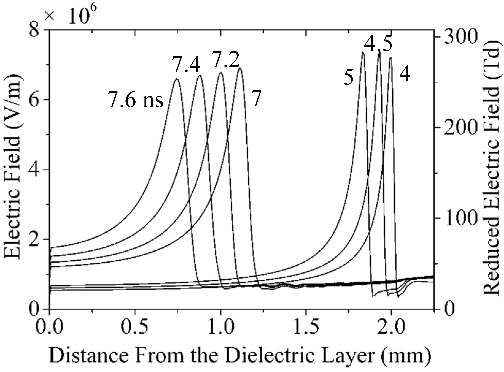
3.1. Electric Field Distribution and Streamer Propagation Velocity

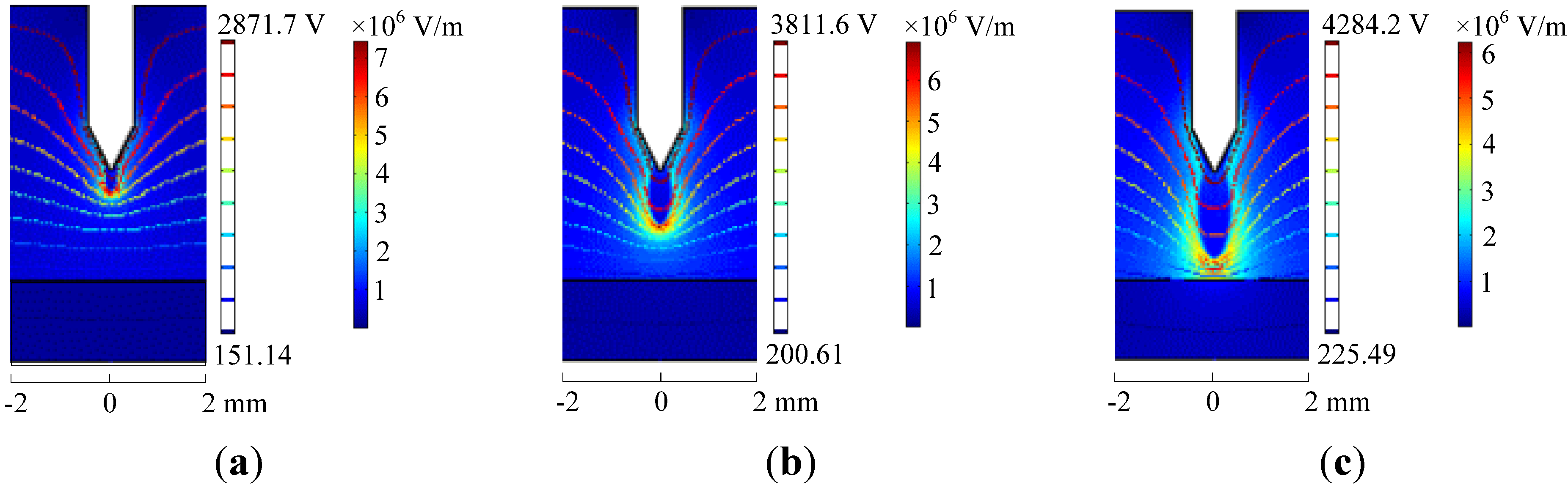
Figure 5 shows the 2-D structure of the absolute value of the electric field at 5, 7, and 8.1 ns in SNG. Figure 6 shows the electric field distribution along the axis of the streamer propagation of the SNG.

Figure 5. Electric field distribution of a cross section for the SNG: (a) 5 ns; (b) 7 ns; (c) 8.1 ns.

Figure 5. Electric field distribution of a cross section for the SNG: (a) 5 ns; (b) 7 ns; (c) 8.1 ns.

Figure 6. Electric field distribution along the axis of the streamer propagation of the SNG at different times.

Figure 6. Electric field distribution along the axis of the streamer propagation of the SNG at different times.

Generally, when the applied electric field is larger than the local breakdown field strength, the electron drift velocity can reach 2 × 10⁷ cm/s, whereas the positive ion drift velocity can be approximately 2 × 10⁵ cm/s [63]. Under the applied electric field effect, the seed electrons begin to drift and multiply until they reach the anode. Growing electrons produce a high space charge where self-propagating streamers are formed, and the applied electric field in the streamer head is largely increased. Consequently, the simulation results in the current work (Figure 5) indicate that the classic structure of a positive streamer discharge is divided into a streamer head, which propagates with a high electric field toward the dielectric layer, and a streamer channel, which corresponds to a highly conductive channel connecting the streamer head to the anode (needle). In addition, Figure 5 demonstrates that the largest electric field always appears at the streamer head, and the electric field along the axial symmetry line is reduced dramatically after the streamer passes any point. The electric field near the anode ranges from 0.8 × 10⁶ V/m to 0.95 × 10⁶ V/m (shown in the corresponding dark-blue region). This value is in accordance with the discharge theory that states that the electric field gradually tends to (1–2) × 10⁶ V/m in the streamer channel [64]. The electric field at the streamer head is within the 6.6 × 10⁶–7.4 × 10⁶ V/m range, slightly smaller than that reported in [65] (within the 1 × 10⁷–1.83 × 10⁷ V/m range). The electric field near the cathode ranges from 0.6 × 10⁶ V/m to 1.8 × 10⁶ V/m.

During the streamer propagation, the electric field at the streamer head increased first, attained its highest value at 4.5 ns, and reduced gradually. This trend was consistent with that in [66] where the point-to-plane gap is 1 mm.

In Figure 6, the simulation results show that the streamer propagates nearly one-half of the air gap in the first 7 ns, and the average velocity during the first 7 ns is approximately 1.6 × 10⁵ m/s. In the next 1 ns, the streamer propagates to 0.7 mm, and the average velocity is 7 × 10⁵ m/s. During the 8–8.1 ns time, the streamer travels 0.1 mm, and the average velocity is nearly 10⁶ m/s. This result is consistent with the reported experimental results by Yi and Williams [67]. They observed the streamer propagation of the needle-to-plane geometry produced in a short gap (0.5–1 cm) using high-speed photography. Their experimental results revealed that the speed of the streamer propagation increased as the propagation developed, and the speed reached up to approximately 10⁶ m/s. Ono [6] photographed a streamer discharge in a 5 mm-air-gap using a short-gated ICCD camera, where atmospheric pressure and 300 °C were adopted. The experimental results showed the steamer reached the cathode in 7 ns, and the average velocity was around 7.14 × 10⁵ m/s. According to the experimental results in [67], the values of the speed deduced from various empirical formulas differed by almost one order of magnitude, even under the same experimental condition. In addition, experimental conditions (including gas, gap lengths, and electric field strengths) significantly affect the streamer propagation. Therefore, the simulation results in the current work can be concluded as reasonable.

The electric field distribution of the TNG investigated using hydrodynamic model is shown in Figure 7 and Figure 8. For clarity, two definitions are introduced in the TNG: (1) The needle electrode located at r = 0, i.e., the middle needle, is labeled as MN. (2) The needle electrodes located at r = 5 mm, i.e., the side needle electrodes, are labeled as SNs.

With the streamer propagation, both the electric fields at the head of the streamer from MN and that from SNs increase at first, then decrease and increase gradually. They reach their greatest value also at 4.5 ns. But under the impact of mutual effect of nearby needles, the distribution of the electric field for TNG is different from that for the SNG. The electric fields at the streamer head of MN and SNs in TNG decrease compared with that in SNG. It is in the 4.7 × 10⁶ V/m to 6.8 × 10⁶ V/m range at the streamer head of MN, and that of the SN is in the 2.56 × 10⁶ V/m to 3.3 × 10⁶ V/m range. The electric field near the cathode of MN ranges from 0.6 × 10⁶ V/m to 1.45 × 10⁶ V/m, and that of the SN ranges from 0.7 × 10⁶ V/m to 1.8 × 10⁶ V/m.

Figure 7. Electric field distribution of a cross section of the TNG: (a) 5 ns; (b) 7 ns; (c) 8.1 ns (the cross section in the dashed frame is the section in Figure 9); (d) 8.5 ns.

Figure 7. Electric field distribution of a cross section of the TNG: (a) 5 ns; (b) 7 ns; (c) 8.1 ns (the cross section in the dashed frame is the section in Figure 9); (d) 8.5 ns.

Figure 8. The electric field distribution along axis in streamer propagation for TNG at various times: (a) MN; (b) SN.

Figure 8. The electric field distribution along axis in streamer propagation for TNG at various times: (a) MN; (b) SN.

It is also noticed that the electric fields in the streamer channels from MN and SNs are approaching to 1 × 10⁶ V/m, which is similar to the situation of the SNG, except those from SNs at 4 ns, 4.5 ns and 5 ns. They hardly vary with the distance from the dielectric layer, whereas those in the streamer channels at 4 ns, 4.5 ns and 5 ns increase with the distance, ranging from 0.25 × 10⁶ V/m to 0.55 × 10⁶ V/m. As it mentioned previously, the streamers from SN propagate relatively slow at the first 5 ns. In this case, the positive ions leave the anode for a short distance (0.25 mm at 5 ns), whereas the electrons have entered the anode. Thus, the applied electric field near the anode is affected much by the space charges, and it varies with the distance from the dielectric layer.

Under the impact of mutual effect between nearby needles, the propagation velocities of MN and SNs in the multi-needle model are different from that in the SNG. As to the streamer from the MN, it propagates less than 1/2 air gap in the first 7 ns, and the average velocity of the first 7 ns is about 1.2 × 10⁵ m/s, the average velocity in 7–8 ns is about 5.5 × 10⁵ m/s, and the average velocity of the propagation during 8–8.7 ns is approximately 10⁶ m/s. As to the streamer from SN, it propagates 0.8 mm in the first 7 ns and the average velocity of the propagating is 1.2 × 10⁵ m/s; in the following 1 ns, the streamer propagates 0.75 mm and the average velocity is 7.5 × 10⁵ m/s; in the period of 8–8.1 ns, the streamer travels 0.1 mm and the average velocity is nearly 10⁶ m/s. This is consistent with the reported experimental results by Won J Yi and P F Williams [67].

It is seen that, without the effect of other needles, the streamer in SNG propagates most quickly (Figure 5 and Figure 6). It takes 8.2 ns for the streamer in the SNG to bridge the air gap. However, it takes 8.3 ns for the streamer from NEs to bridge the air gap, and 8.7 ns for the streamer from MN. This shows that the mutual effect between neighboring needles influences the streamer velocities.

The different simulation patterns between SNG and TNG shown in Figure 5, Figure 6, Figure 7 and Figure 8 result from the mutual effect of nearby needles. The potential isolines around the needle tip in SNG tended to be steeper than those of MN in TNG at the same instant. That is, the corona-like character is stronger in SNG than in TNG. In this case, the maximum value of the electric field at the streamer head in SNG exceeds 7.4 × 10⁶ V/m, while that of the MN in TNG is approximately 6.5 × 10⁶ V/m. Similarly, the maximum values of the electric fields at the streamer heads in SNG are greater than those of MN in TNG. Therefore, the total electric field gets to be more uniform in TNG that the corona-like character is weakened. When the gas pressure (or the gas density) is fixed, electron mean free path, and the collision frequency between electrons and other particles are considered nearly constant. Greater E/N, i.e., greater E, leads to more energy that the electron obtained from the applied electric field. Then the energy transferred to other particles from electrons through collision increases as well. So, the ionized and excited gas molecules increase macroscopically, and the velocity of streamer propagation increases.

Evidently, the three streamer (the streamer in SNG, the streamers of MN and SN in TNG) propagations have a common feature, i.e., they propagate more and more quickly. As to the streamer of SNG, the amplitude value of the applied voltage, the voltage at the streamer head and the distance from the dielectric layer at different times is given in Table 4. From the table, it could be seen that the unbridged air gap becomes shorter, whereas the potential at the head of the streamer does not decrease clearly when the streamer propagates. Therefore, the electric field strength at the streamer head increases, resulting in the increase in propagation velocity.

Further, the computed patterns of the electric field distribution for the SN were not symmetrical, whereas those for the MN were symmetrical (Figure 7), which also illustrates that the interaction of adjacent needles played a significant role in streamer propagation. Meanwhile, the z component of potential gradient along the axis in streamer propagation of MN is greater than that of SN, especially in the domain around the streamer head (Figure 9). The z component of potential gradient could be roughly defined as Δφ/Δz, in which Δφ is the potential difference between two adjacent potential isolines, and Δz is the distances between the points of intersection of adjacent potential isolines and the axis in streamer propagation. For the points of intersection of potential isolines with the values of 3382.3 V, 3931.3 V, 2480.4 V and r = 0, the absolute values of the z component of potential gradient are 3.7 × 10⁶ V/m, 4.5 × 10⁶ V/m and 3.47 × 10⁶ V/m respectively. However, for the points of intersection of the same potential isolines and r = −5, the absolute values of the z component of potential gradient are 1.96 × 10⁶ V/m, 2.5 × 10⁶ V/m and 2.05 × 10⁶ V/m respectively. Therefore, the electric fields at the streamer head of MN are greater of than those of SNs. As mentioned previously, the potential isolines around the needle tip in SNG tended to be steeper than those of MN in TNG at the same instant. Similarly, the increase in the z component of potential gradient of TNG leads to greater electric fields at the streamer head compared with those of MN and SNs in SNG.

Table 4. The amplitude value of the applied voltage, the voltage at the streamer head and the distance from the dielectric layer at different times for SNG.

Time (ns)	The amplitude value of the applied voltage (V)	Calculated voltage at the streamer head (V)	Distance from the dielectric layer (mm)
5	2871.7	2267.2	1.85
7	3811.6	2206.7	1.1
8.1	4284.2	1578.4	0.4

Table 4. The amplitude value of the applied voltage, the voltage at the streamer head and the distance from the dielectric layer at different times for SNG.

Time (ns)	The amplitude value of the applied voltage (V)	Calculated voltage at the streamer head (V)	Distance from the dielectric layer (mm)
5	2871.7	2267.2	1.85
7	3811.6	2206.7	1.1
8.1	4284.2	1578.4	0.4

Figure 9. Electric field and potential isoline distribution of partial domain in MNG.

Figure 9. Electric field and potential isoline distribution of partial domain in MNG.

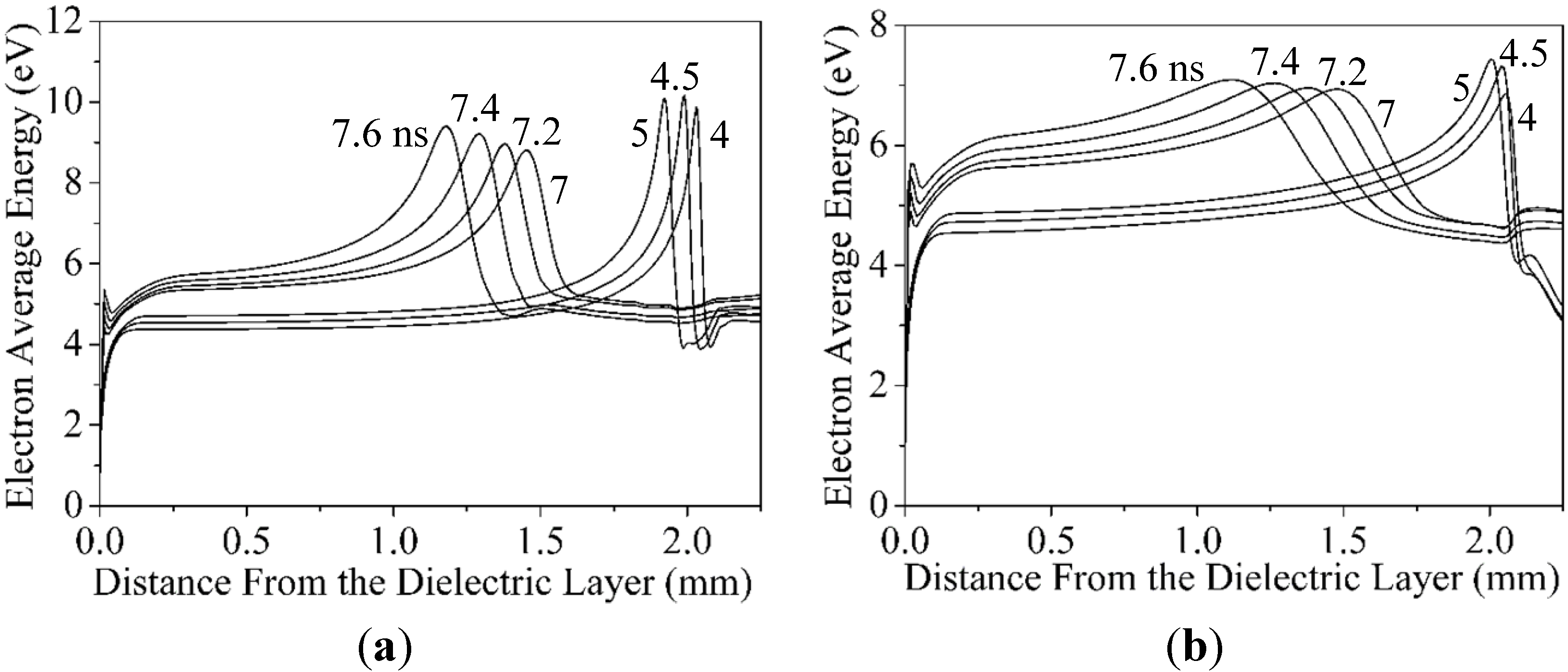
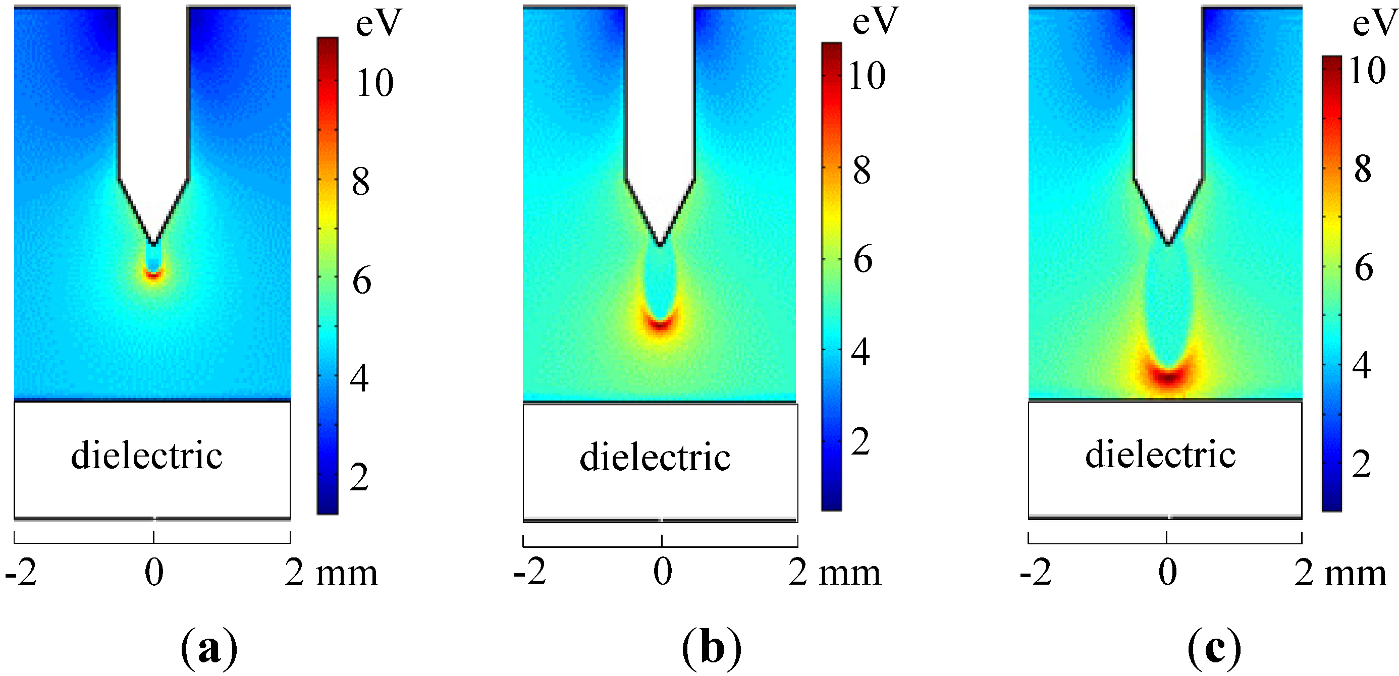
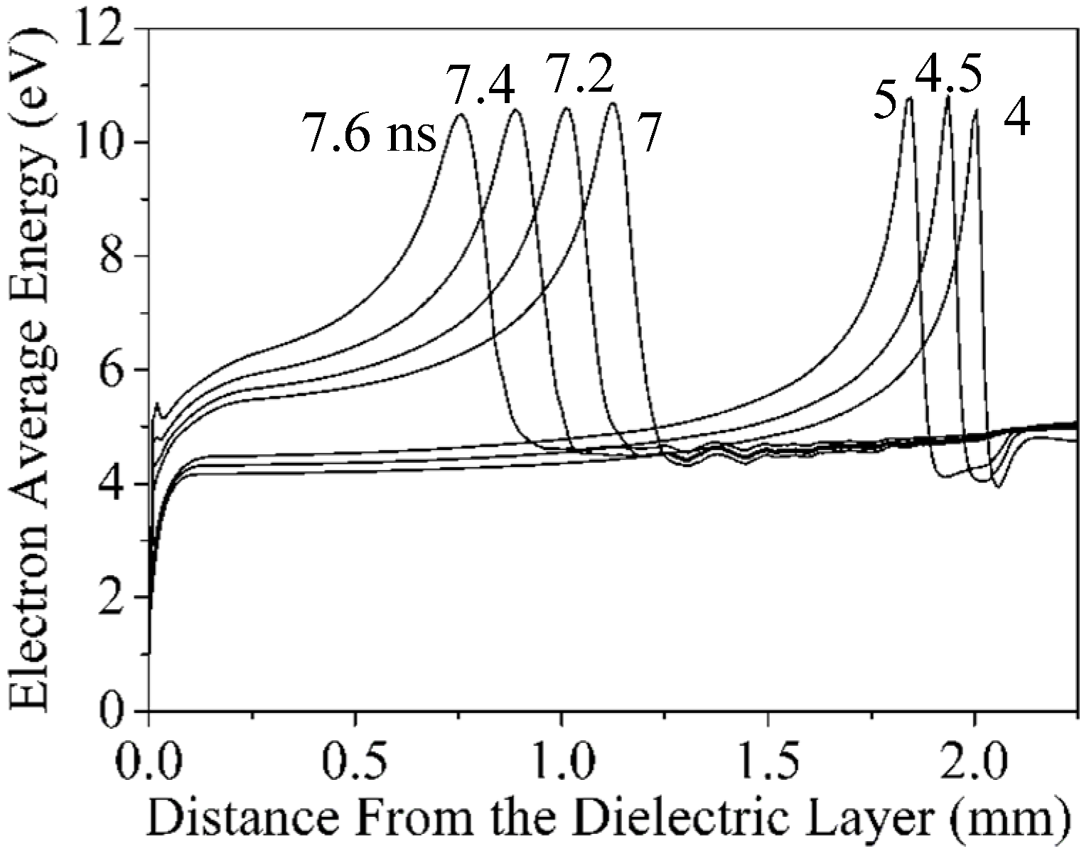
3.2. Electron Average Energy Profile

Figure 10, Figure 11, Figure 12 and Figure 13 show the electron average energy profile obtained through hydrodynamic model for the SNG and the TNG. In Figure 10 and Figure 11, the electron average energy in the streamer channel is approximately 5 eV, which ranges from 10.4 eV to 10.8 eV at the streamer head and from 5 eV to 8 eV in the unbridged gap, with reduced electric field ranging from 250 Td to 285 Td (Figure 6). Sigmond [68] estimated that the electron average energy in the streamer head ranges from 12 eV to 16 eV when the reduced electric field of the streamer head ranged from 400 Td to 600 Td. Sima et al. [65] reported that the electron average energy in the streamer head was from 13 eV to 22 eV with the reduced electric field ranging from 430 Td to 800 Td. These values are slightly smaller than those reported in the current paper.

Figure 10. Electron average energy profile over the axial cross section of the SNG: (a) 5 ns; (b) 7 ns; (c) 8.1 ns.

Figure 10. Electron average energy profile over the axial cross section of the SNG: (a) 5 ns; (b) 7 ns; (c) 8.1 ns.

Figure 11. Electron average energy along the axis of symmetry for the SNG.

Figure 11. Electron average energy along the axis of symmetry for the SNG.

Figure 12 and Figure 13 show that the variations of the electron average energy come out to be different from those in Figure 10 and Figure 11 under the mutual effect of nearby needles. For the MN, the electron average energy in the streamer channel is around 4.5–5 eV (which ranges from 8.8 eV to 10.2 eV at the streamer head) and from 4.5 eV to 6 eV in the unbridged gap. For the SN, the electron average energy at the streamer head ranges from 6.8 eV to 7.4 eV and from 4.5 to 6.5 eV in the unbridged gap.

Figure 12. Electron average energy profile over the axial cross section of the TNG: (a) 5 ns; (b) 7 ns; (c) 8.1 ns; (d) 8.5 ns.

Figure 12. Electron average energy profile over the axial cross section of the TNG: (a) 5 ns; (b) 7 ns; (c) 8.1 ns; (d) 8.5 ns.

Figure 13. Electron mean energy variation along the axis of the streamer propagation of the TNG: (a) MN; (b) SN.

Figure 13. Electron mean energy variation along the axis of the streamer propagation of the TNG: (a) MN; (b) SN.

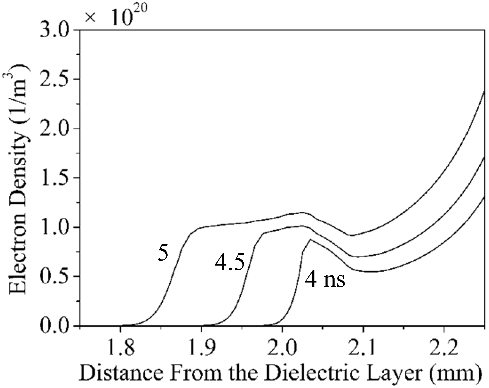
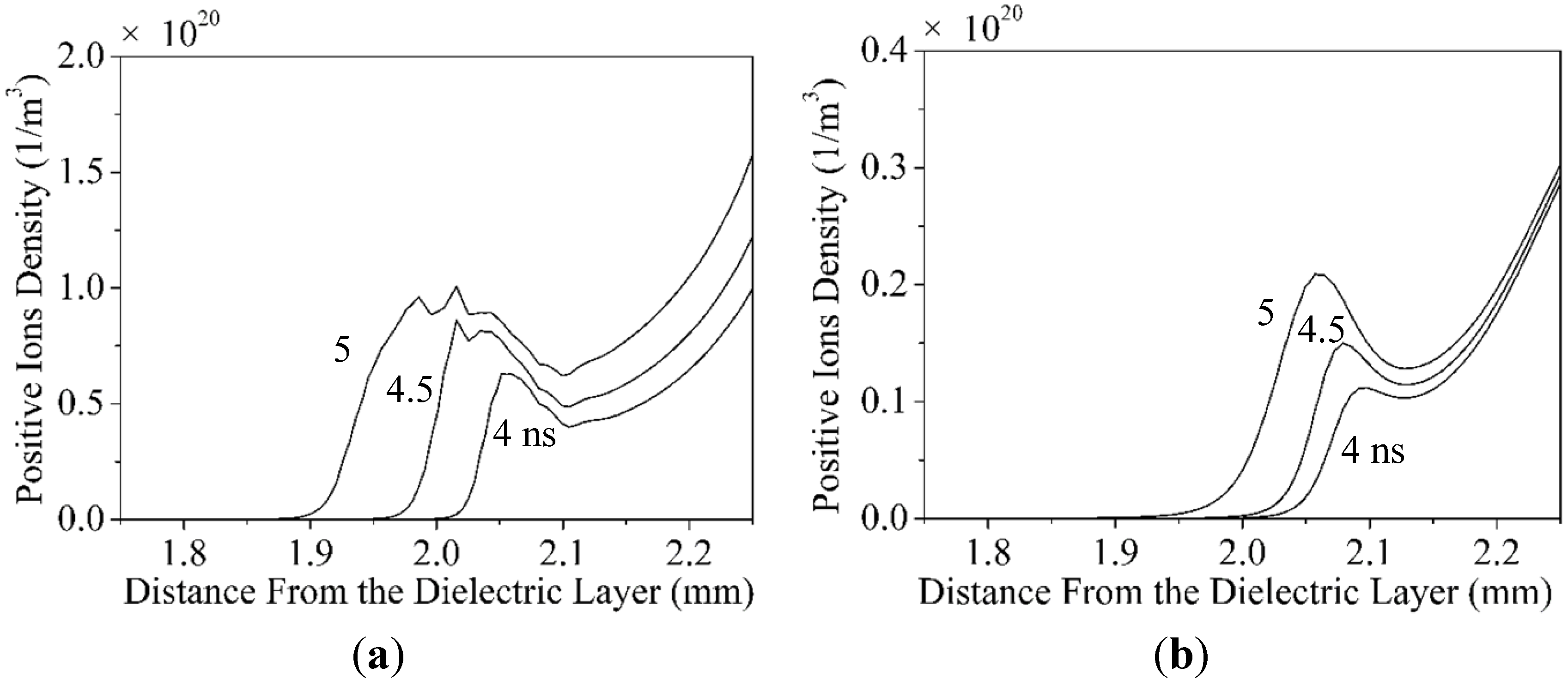
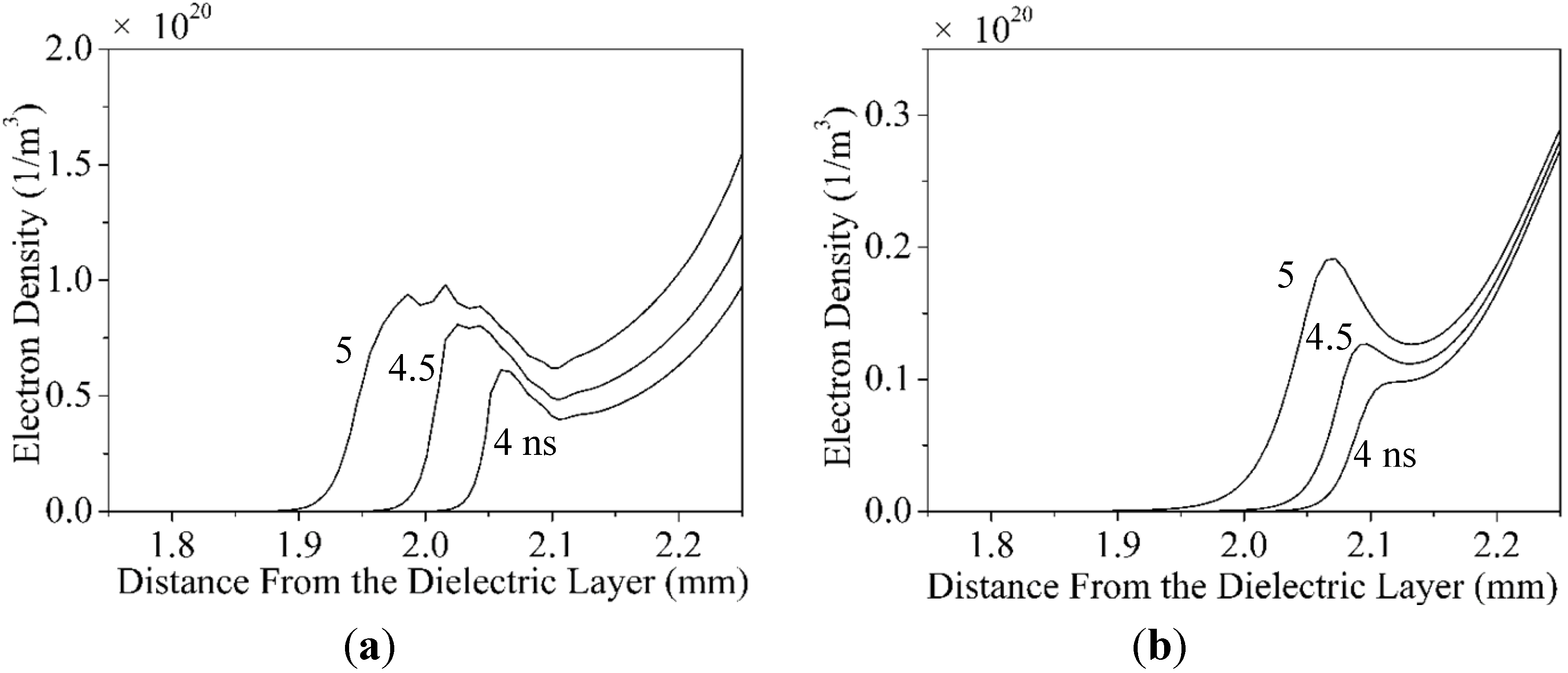
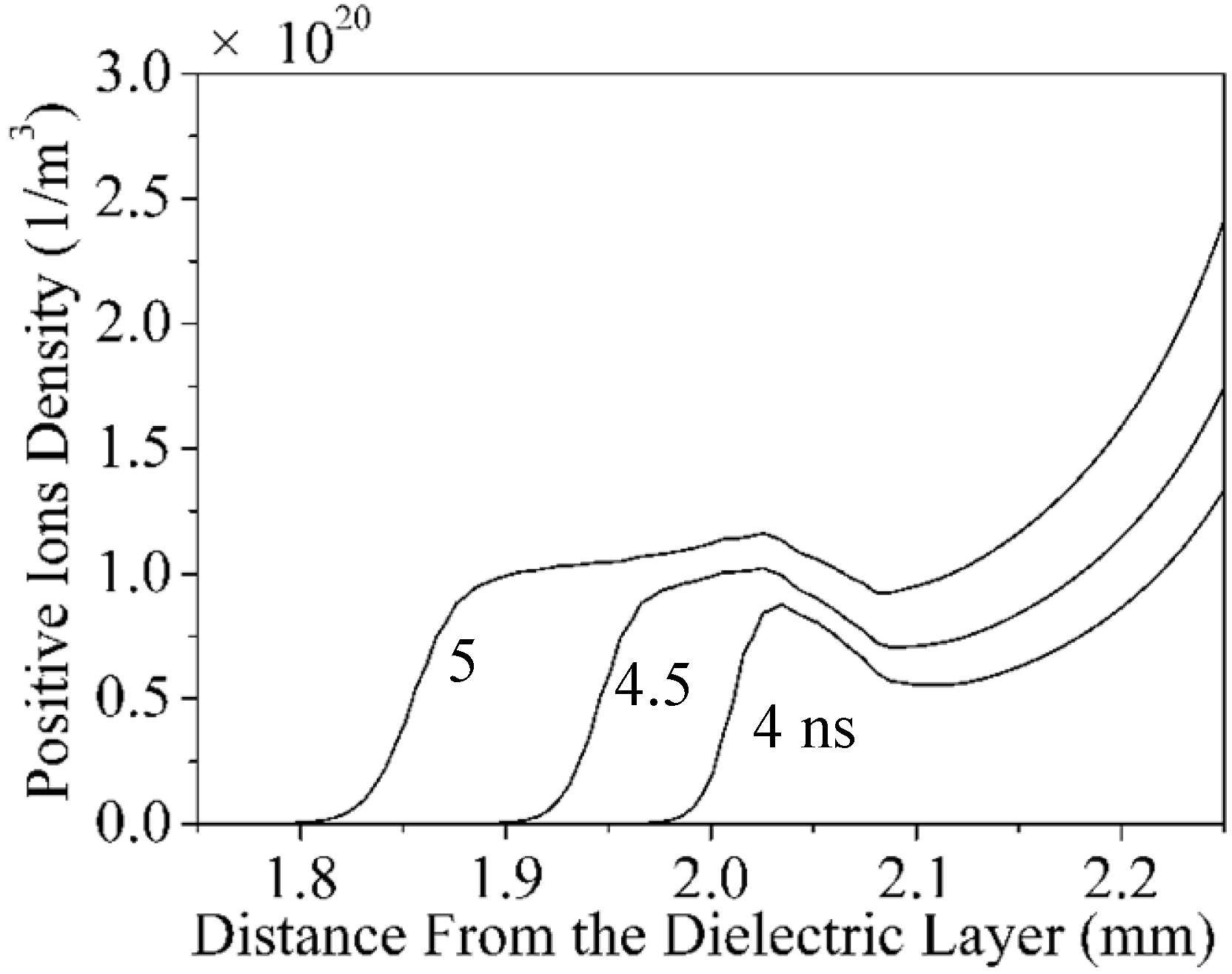
3.3. Distribution of Electron and Positive Ions

Figure 14 shows the calculated electron density distribution in the streamer discharge for the SNG. The electron number density reaches the local extremum in the region near the anode and at the head of the streamer. In the streamer channel, the electron density decreases in the direction of the streamer propagation in the 2.08–2.25 mm region away from the dielectric layer at 5 ns, whereas it increases along the same direction in the other regions.

Figure 14. Electron density distribution (1/m³) along the axis of symmetry of the SNG.

Figure 14. Electron density distribution (1/m³) along the axis of symmetry of the SNG.

In the region near the needle electrode, the applied electric field is large, which leads to severe ionization and electron multiplication. In addition, streamer formation needs space charges to distort the space field. The superposition of the space charge field and the applied field in the region is about (0.7–1) × 10⁶ V/m (Figure 6). Considering that the applied electric field is large, more space charges are needed to counteract the applied one. Therefore, the electrons density reaches the local extremum in this region.

As mentioned earlier, the unbridged air gap by streamer became shorter, whereas the potential at the head of the streamer did not decrease obviously with streamer propagation. Therefore, the electric field strength at the streamer head increased, resulting in more severe ionization and greater electron number density. However, the smaller electric field in the streamer channel produced more attachment of electrons to the molecules. Thus, the electron number density decreased in the channel.

The calculated electron density range at the head of the streamer was at (0.88–1.12) × 10²⁰ 1/m³ at 4–5 ns, which agreed with the 10²⁰–10²² 1/m³ value estimated in [69].

It could be seen from Figure 15 that, under the mutual effect of the SN, the electron density at the streamer head of MN in the TNG decreased slightly compared with that in the SNG, within the range of (0.65–1.0) × 10²⁰ 1/m³ during 4–5 ns. The electron density at the streamer head of the SN decreased also, in the range of (0.09–0.18) × 10²⁰ 1/m³, during the same period.

Figure 15. Electron density distribution (1/m³) along the axis of symmetry of the TNG: (a) MN; (b) SN.

Figure 15. Electron density distribution (1/m³) along the axis of symmetry of the TNG: (a) MN; (b) SN.

Figure 16 and Figure 17 show the positive ion density distribution in the streamer discharge for the SNG. The positive ion number density reaches the local extremum in the region near the anode and at the head of the streamer. In the streamer channel, the positive ion density decreases in the direction of the streamer propagation in the 2.08–2.25 mm region away from the dielectric layer at 5 ns, whereas it increases along the same direction in the other regions.

Figure 16. Positive ion density distribution along the axis of symmetry of the SNG.

Figure 16. Positive ion density distribution along the axis of symmetry of the SNG.

Figure 17. Positive ion density distribution along the axis of symmetry of the TNG: (a) MN; (b) SN.

Figure 17. Positive ion density distribution along the axis of symmetry of the TNG: (a) MN; (b) SN.

4. Conclusions

A 2-D fluid-hydrodynamic numerical modelling of a DBD for multi-needle configuration in a 2.25 mm-gap at atmospheric pressure has been performed. In the simulation, the impulse voltage with a peak value of 10.6 kV, specified rise time of 0.05 μs, and a decay to half the peak value in 0.2 μs was applied.

Comparison of the theoretical results between the single-needle and three-needle geometries was also performed. The simulation results demonstrated that the mutual effect of nearby needles influences the DBD characteristics.

(1) Under the mutual effect of nearby needles, the decrease in potential gradient caused that electric fields at the streamer head of MN and SNs in the TNG decreased compared with those in the single-needle model. Similarly, the difference of the electric fields between MN and SNs also resulted from different potential gradient. They were in the 4.7 × 10⁶–6.8 × 10⁶ V/m range at the MN streamer head, and those of SNs were in the 2.56 × 10⁶–3.3 × 10⁶ V/m range.

(2) The average propagation velocities of the streamers from MN and SNs were slightly slower than that of the single-needle model, especially during the initial stage of the propagation, resulting from the mutual effect. In the three streamers, the average propagation velocities all approached 10⁶ m/s during the final period of the propagation.

(3) The electron average energy profiles of MN and SNs, i.e., in the streamer channel, at the streamer head, and in the unbridged gap, decreased slightly because of the mutual effect.

(4) The electron density at the MN streamer head and that of the SN decreased compared with that of the single-needle geometry.

By comparison, the results obtained in the current paper were in good agreement with the experimental and simulation results in literature, which also indicated that numerical modelling is both powerful and necessary in investigating the DBD mechanism.

References

1. Kogelschatz, U. Dielectric-barrier discharges: Their history, discharge physics, and industrial applications. Plasma Chem. Plasma Process. 2003, 23, 1–46. [Google Scholar] [CrossRef]
2. Palaskar, S.; Kale, K.H.; Nadiger, G.S.; Desai, A.N. Dielectric barrier discharge plasma induced surface modification of polyester/cotton blended fabrics to impart water repellency using HMDSO. J. Appl. Polym. Sci. 2011, 122, 1092–1100. [Google Scholar] [CrossRef]
3. De Geyter, N.; Morent, R.; van Vlierberghe, S.; Frere-Trentesaux, M.; Dubruel, P.; Payen, E. Effect of electrode geometry on the uniformity of plasma-polymerized methyl methacrylate coatings. Prog. Org. Coating 2011, 70, 293–299. [Google Scholar] [CrossRef]
4. An, H.T.Q.; Huu, T.P.; Le van, T.; Cormier, J.M.; Khacef, A. Application of atmospheric non thermal plasma-catalysis hybrid system for air pollution control: Toluene removal. Catal. Today 2010, 176, 474–477. [Google Scholar]
5. Rong, M.; Liu, D.; Wang, D.; Su, B.; Wang, X.; Wu, Y. A new structure optimization method for the interneedle distance of a multineedle-to-plane barrier discharge reactor. IEEE Trans. Plasma Sci. 2010, 38, 966–972. [Google Scholar] [CrossRef]
6. Ono, R.; Oda, T. Ozone production process in pulsed positive dielectric barrier discharge. J. Phys. D Appl. Phys. 2007, 40, 176–182. [Google Scholar] [CrossRef]
7. Daou, F.; Vincent, A.; Amouroux, J. Point and multipoint to plane barrier discharge process for removal of NOx from engine exhaust gases: Understanding of the reactional mechanism by isotopic labeling. Plasma Chem. Plasma Process. 2003, 23, 309–325. [Google Scholar] [CrossRef]
8. Dang, X.Q.; Huang, J.Y.; Chen, L.; Liu, X.; Kang, L. Research on removal of dilute gaseous toluene using dielectric barrier discharge with TiO2 photocatalyst. In Proceedings of the 2010 IEEE International Conference on Mechanic Automation and Control Engineering, Wuhan, China, 26–28 June 2010; pp. 2026–2031.
9. Wang, X.; Sun, C. Formation conditions for transported charges of multineedle-to-cylinder dielectric barrier discharge based on the orthogonal design and lissajous figures. In Proceedings of the 2011 International Conference on Information Science and Engineering Application, Chongqing, China, 21–23 October 2011.
10. Bhoj, A.N.; Kushner, M.J. Multi-scale simulation of functionalization of rough polymer surfaces using atmospheric pressure plasmas. J. Phys. D Appl. Phys. 2006, 39, 1594–1598. [Google Scholar] [CrossRef]
11. Wang, X.; Yang, Q.; Yao, C.; Zhang, X.; Sun, C. Dielectric barrier discharge characteristics of multineedle-to-cylinder configuration. Energies 2011, 4, 2133–2150. [Google Scholar] [CrossRef]
12. Takaki, K.; Fujiwara, T. Multipoint barrier discharge process for removal of NOx from diesel engine exhaust. IEEE Trans. Plasma Sci. 2001, 29, 518–523. [Google Scholar] [CrossRef]
13. Takaki, K.; Jani, M.A.; Fujiwara, T. Removal of nitric oxide in flue gases by multipoint to plane dielectric barrier discharge. IEEE Trans. Plasma Sci. 1999, 27, 1137–1145. [Google Scholar] [CrossRef]
14. Jani, M.A.; Takaki, K.; Fujiwara, T. Low-voltage operation of a plasma reactor for exhaust gas treatment by dielectric barrier discharge. Rev. Sci. Instr. 1998, 69, 1847–1849. [Google Scholar] [CrossRef]
15. Jani, M.A.; Takaki, K.; Fujiwara, T. Streamer polarity dependence of NOx removal by dielectric barrier discharge with a multipoint-to-plane geometry. J. Phys. D Appl. Phys. 1999, 32, 2560–2567. [Google Scholar] [CrossRef]
16. Zhou, B.; Wang, X.-J.; Sun, C.-X. Effect of electrode structure on the parameters of dielectric barrier discharge. High Volt. Appl. 2010, 46, 31–34. [Google Scholar]
17. Kang, W.S.; Park, J.M.; Kim, Y.; Hong, S.H. Numerical study on influences of barrier arrangements on dielectric barrier discharge characteristics. IEEE Trans. Plasma Sci. 2003, 31, 504–510. [Google Scholar] [CrossRef]
18. Massines, F.; Segur, P.; Gherardi, N.; Khamphan, C.; Ricard, A. Physics and chemistry in a glow dielectric barrier discharge at atmospheric pressure: Diagnostics and modelling. Surf. Coat. Technol. 2003, 174, 8–14. [Google Scholar] [CrossRef]
19. Dorai, R.; Kushner, M.J. A model for plasma modification of polypropylene using atmospheric pressure discharges. J. Phys. D Appl. Phys. 2003, 36, 666–685. [Google Scholar] [CrossRef]
20. Massines, F.; Rabehi, A.; Decomps, P.; Gadri, R.B.; Segur, P.; Mayoux, C. Experimental and theoretical study of a glow discharge at atmospheric pressure controlled by dielectric barrier. J. Appl. Phys. 1998, 83, 2950–2957. [Google Scholar] [CrossRef]
21. Kogelschatz, U. Filamentary, patterned, and diffuse barrier discharges. IEEE Trans. Plasma Sci. 2002, 30, 1400–1408. [Google Scholar] [CrossRef]
22. Babaeva, N.Y.; Kushner, M.J. Intracellular electric fields produced by dielectric barrier discharge treatment of skin. J. Phys. D Appl. Phys. 2010, 43, 185206. [Google Scholar] [CrossRef]
23. Georghiou, G.E.; Papadakis, A.P.; Morrow, R.; Metaxas, A.C. Numerical modelling of atmospheric pressure gas discharges leading to plasma production. J. Phys. D Appl. Phys. 2005, 38, R303–R328. [Google Scholar] [CrossRef]
24. Babaeva, N.Y.; Kushner, M.J. Ion energy and angular distributions onto polymer surfaces delivered by dielectric barrier discharge filaments in air: I. Flat surfaces. Plasma Sources Sci. Technol. 2011, 20, 035017–035027. [Google Scholar] [CrossRef]
25. Zhuang, Y.; Chen, G.; Rotaru, M. Numerical modelling of needle-grid electrodes for negative surface corona charging system. J. Phys. Conf. Ser. 2011, 310. [Google Scholar] [CrossRef]
26. Kumara, S.; Serdyuk, Y.V.; Gubanski, S.M. Charging of polymeric surfaces by positive impulse corona. IEEE Trans. Dielect. Electr. Insul. 2009, 16, 726–733. [Google Scholar] [CrossRef]
27. Storch, D.G.; Kushner, M.J. Destruction mechanisms for formaldehyde in atmospheric-pressure low-temperature plasmas. J. Appl. Phys. 1993, 73, 51–55. [Google Scholar] [CrossRef]
28. Georghiou, G.E.; Morrow, R.; Metaxas, A.C. The effect of photoemission on the streamer development and propagation in short uniform gaps. J. Phys. D Appl. Phys. 2001, 34, 200–208. [Google Scholar] [CrossRef]
29. Kushner, M.J. Hybrid modelling of low temperature plasmas for fundamental investigations and equipment design. J. Phys. D Appl. Phys. 2009, 42, 194013–194032. [Google Scholar] [CrossRef]
30. Raether, H. Development of electron avalanche in the radio channel. Zeitschrift Fur Physik 1939, 112, 464–489. [Google Scholar] [CrossRef]
31. Loeb, L.B.; Meek, J.M. The mechanism of spark discharge in air at atmospheric pressure. I. J. Appl. Phys. 1940, 11, 438–447. [Google Scholar] [CrossRef]
32. Li, C.; Ebert, U.; Hundsdorfer, W. Spatially hybrid computations for streamer discharges: II. Fully 3D simulations. J. Comput. Phys. 2012, 231, 1020–1050. [Google Scholar] [CrossRef]
33. Li, C.; Ebert, U.; Hundsdorfer, W. Spatially hybrid computations for streamer discharges with generic features of pulled fronts: I. Planar fronts. J. Comput. Phys. 2010, 229, 200–220. [Google Scholar] [CrossRef] [Green Version]
34. Li, C.; Ebert, U.; Hundsdorfer, W. 3D hybrid computations for streamer discharges and production of runaway electrons. J. Phys. D Appl. Phys. 2009, 42, 202003:1–4: 202003. [Google Scholar]
35. Li, C.; Ebert, U.; Brok, W.J.M.; Hundsdorfer, W. Spatial coupling of particle and fluid models for streamers: where nonlocality matters. J. Phys. D Appl. Phys. 2008, 41, 032005:1–4:032005. [Google Scholar]
36. Li, C.; Brok, W.J.M.; Ebert, U.; van der Mullen, J.J.A.M. Deviations from the local field approximation in negative streamer heads. J. Appl. Phys. 2007, 101, 123305:1–17:123305. [Google Scholar]
37. Farouk, T.; Farouk, B.; Staack, D.; Gutsol, A.; Fridman, A. Simulation of dc atmospheric pressure argon micro glow-discharge. Plasma Sources Sci. Technol. 2006, 15, 676–688. [Google Scholar] [CrossRef]
38. Pancheshnyi, S.; Nudnova, M.; Starikovskii, A. Development of a cathode-directed streamer discharge in air at different pressures: Experiment and comparison with direct numerical simulation. Phys. Rev. E 2005, 71, 016407:1–12:016407. [Google Scholar] [CrossRef]
39. Georghiou, G.E.; Morrow, R.; Metaxas, A.C. Two-dimensional simulation of streamers using the FE-FCT algorithm. J. Phys-D-Appl. Phys. 2000, 33, L27–L32. [Google Scholar]
40. Georghiou, G.E.; Morrow, R.; Metaxas, A.C. An improved finite-element flux-corrected transport algorithm. J. Comput. Phys. 1999, 148, 605–620. [Google Scholar] [CrossRef]
41. Nagayama, K.; Farouk, B.; Lee, Y.H. Particle simulation of radio-frequency plasma discharges of methane for carbon film deposition. IEEE Trans. Plasma Sci. 1998, 26, 125–134. [Google Scholar] [CrossRef]
42. Morrow, R.; Lowke, J.J. Streamer propagation in air. J. Phys-D-Appl. Phys. 1997, 30, 614–627. [Google Scholar]
43. Nagayama, K.; Farouk, B.; Lee, Y.H. Neutral and charged particle simulation of RF Ar plasma. Plasma Sources Sci. Technol. 1996, 5, 685–695. [Google Scholar] [CrossRef]
44. Bourdon, A.; Pasko, V.P.; Liu, N.Y.; Célestin, S.; Segur, P.; Marode, E. Efficient models for photoionization produced by non-thermal gas discharges in air based on radiative transfer and the Helmholtz equations. Plasma Sources Sci. Technol. 2007, 16, 656–678. [Google Scholar] [CrossRef]
45. Célestin, S.; Bonaventura, Z.; Zeghondy, B.; Bourdon, A.; Ségur, P. Influence of surface charges on the structure of a dielectric barrier discharge in air at atmospheric pressure: Experiment and modeling. Eur. Phys. J. Appl. Phys. 2009, 47. [Google Scholar] [CrossRef]
46. Célestin, S.; Bonaventura, Z.; Zeghondy, B.; Bourdon, A.; Ségur, P. The use of the ghost fluid method for Poisson's equation to simulate streamer propagation in point-to-plane and point-to-point geometries. J. Phys. D Appl. Phys. 2009, 42, 065203:1–14:065203. [Google Scholar]
47. Guo, J.-M.; Wu, C.-H.J. Two-dimensional nonequilibrium fluid models for streamers. IEEE Trans. Plasma Sci. 1993, 21, 684–695. [Google Scholar] [CrossRef]
48. Eichwald, O.; Ducasse, O.; Merbahi, N.; Yousfi, M.; Dubois, D. Effect of order fluid models on flue gas streamer dynamics. J. Phys. D Appl. Phys. 2006, 39, 99–107. [Google Scholar] [CrossRef]
49. Sakiyama, Y.; Graves, D.B. Finite element analysis of an atmospheric pressure RF-excited plasma needle. J. Phys. D Appl. Phys. 2006, 39, 3451–3456. [Google Scholar] [CrossRef]
50. Dhali, S.K.; Williams, P.F. Two-Dimensional Studies of Streamers in Gases. J. Appl. Phys. 1987, 62, 4696–4707. [Google Scholar] [CrossRef]
51. Wang, M.C.; Kunhardt, E.E. Streamer dynamics. Phys. Rev. A 1990, 42, 2366–2373. [Google Scholar] [CrossRef] [PubMed]
52. Kulikovsky, A.A. Positive streamer between parallel plate electrodes in atmospheric pressure air. J. Phys. D Appl. Phys. 1997, 30, 441–450. [Google Scholar] [CrossRef]
53. Vitello, P.A.; Penetrante, B.M.; Bardsley, J.N. Simulation of negative-streamer dynamics in nitrogen. Phys. Rev. E 1994, 49, 5574–5598. [Google Scholar] [CrossRef]
54. Pancheshnyi, S.V.; Starikovskaia, S.M.; Starikovskii, A.Y. Role of photoionization processes in propagation of cathode-directed streamer. J. Phys. D Appl. Phys. 2001, 34, 105–115. [Google Scholar] [CrossRef]
55. Liu, N.Y.; Pasko, V.P. Effects of photoionization on propagation and branching of positive and negative streamers in sprites. J. Geophys. Res. Space Phys. 2004, 109(A4), A04301:1–17:A04301. [Google Scholar] [CrossRef]
56. Zheleznyak, M.B.; Mnatsakarian, A.K.; Sizyka, S.V. Photoionization of nitrogen and oxygen mixtures by radiation from gas discharges. High Temp. 1982, 20, 357–362. [Google Scholar]
57. Hagelaar, G.J.M.; Pitchford, L.C. Solving the Boltzmann equation to obtain electron transport coefficients and rate coefficients for fluid models. Plasma Sources Sci. Technol. 2005, 14, 722–733. [Google Scholar] [CrossRef]
58. BOLSIG + 2005 CPAT. Available online: http://www.codiciel.fr/plateforme/plasma/bolsig/bolsig.php (accessed on 30 April 2009).
59. Lee, S.-H.; Lee, S.-Y.; Park, I.-H. Finite-element analysis of corona discharge onset in air with artificial diffusion scheme and under Fowler-Nordheim electron emission. IEEE Trans. Magn. 2007, 43, 1453–1456. [Google Scholar] [CrossRef]
60. Gupta, D.K.; Mahajan, S.; John, P.I. Theory of step on leading edge of negative corona current pulse. J. Phys. D Appl. Phys. 2000, 33, 681–691. [Google Scholar] [CrossRef]
61. Morrow, R. Theory of negative corona in oxygen. Phys. Rev. A 1985, 32, 1799–1809. [Google Scholar] [CrossRef] [PubMed]
62. Pancheshnyi, S.V.; Starikovskii, A.Y. Two-dimensional numerical modelling of the cathode-directed streamer development in a long gap at high voltage. J. Phys. D Appl. Phys. 2003, 36, 2683–2691. [Google Scholar] [CrossRef]
63. Xu, X.; Zhu, D. Gas Discharge Physics; Fudan Univresity Publisher: Shanghai, China, 1996. [Google Scholar]
64. Liang, X.; Chen, C.; Zhou, Y. High Voltage Engineering; Tsinghua University Press: Beijing, China, 2003; pp. 16–22. [Google Scholar]
65. Sima, W.; Peng, Q.; Yang, Q.; Yuan, T.; Shi, J. Study of the characteristics of a streamer discharge in air based on a plasma chemical model. IEEE Trans. Dielect. Electr. Insul. 2012, 19, 660–670. [Google Scholar] [CrossRef]
66. Ducasse, O.; Papageorghiou, L.; Eichwald, O.; Spyrou, N.; Yousfi, M. Critical analysis on two-dimensional point-to-plane streamer simulations using the finite element and finite volume methods. IEEE Trans. Plasma Sci. 2007, 35, 1287–1300. [Google Scholar] [CrossRef]
67. Yi, W.J.; Williams, P.F. Experimental study of streamers in pure N-2 and N-2/O-2 mixtures and an approximate to 13 cm gap. J. Phys. D Appl. Phys. 2002, 35, 205–218. [Google Scholar] [CrossRef]
68. Sigmond, R.S. The residual streamer channel-return strokes and secondary streamers. J. Appl. Phys. 1984, 56, 1355–1370. [Google Scholar] [CrossRef]
69. Raizer, Y.P.; Allen, J.E.; Kisin, V.I. Gas Discharge Physics; Springer-Verlag: Berlin, Germany, 1991; pp. 357–358. [Google Scholar]