1. Introduction
Due to the rapid development of industry, the overuse of fossil fuels results in environmental pollution, greenhouse effects and ecological damage. Adopting renewable and clean energy resources to replace fossil fuels is imperative. Among renewable-energy resources, solar energy attracts more interest owing to its noiseless, pollution-free, non-radioactive, and inexhaustible characteristics. Solar energy is converted into electric power through photovoltaic (PV) panels. The output voltage and the output current of a PV panel vary nonlinearly with irradiation, panel temperature and loading condition. There is a maximum power point (MPP) under certain atmospheric conditions. To draw maximum power from PV panel, a large number of researchers have proposed maximum power point tracking (MPPT) algorithms. Current MPPT algorithms include the voltage feedback method (VFM) [
1], the power feedback method (PFM) [
2,
3,
4], the perturb-and-observe method (POM) [
5,
6,
7], the incremental conductance method (ICM) [
8,
9], the three-point weight comparison method (TPWCM) [
10,
11], the linear approximation method (LAM) [
12], the neural-network-based method (NNBM) [
13], and the fuzzy-logic-control approach (FLCA) [
14,
15].
The VFM is the simplest method for MPPT, which regulates PV arrays terminal voltage to a reference, handling the operation point of a PV arrays near the maximum power point. It is only suitable for some fixed irradiations and temperatures. In the power feedback method, the derivative dP/dV is regarded as a control index. While a controlled output voltage and its corresponding output power can lead the derivative to zero, a maximum power point is achieved. However, more parameters and complicated calculations are required, which increase the difficulty of MPPT. The perturb-and-observe method is widely used in maximum PV power tracking because it is easy to carry out and few measured parameters are required. Even though a maximum PV power point is reached, continued perturbing and observing will still oscillate around the point, resulting in PV power losses, especially under constant or slow variation of atmospheric conditions. To overcome the mentioned drawbacks of the POM, the ICM was developed. In the ICM, the output voltage or current of a PV array is adjusted until an incremental conductance dI/dV just reaches the ratio of PV output current to voltage. Owing to detection errors, the determined incremental conductance hardly agrees with the value of I/V. Another solution to avoid fluctuations about the maximum power point is the TPWCM. In the TPWCM, three measured points are compared and weighted. Once a new weighted result matches the preset one, subsequent comparisons stop. Nevertheless, a complicated procedure is also required, which lowers the dynamic response significantly. The LAM tracks the maximum power point according to the straight line which connects all MPPs under different irradiation conditions. It is easy to implement and locates MPP rapidly. However, the influence of temperature is neglected. The NNBM and the FLCA can fulfill MPPT regardless of atmospheric conditions and PV cell parameters, but sophisticated calculation and microprocessor-based implementation are still needed.
In this paper, a double-linear approximation algorithm (DLAA) is proposed, which can track the maximum power point instantaneously and can be implemented easily. The DLAA is based on the approximation that the trajectories of maximum power point vary linearly with irradiation and temperature. According to the DLAA, MPPT can be achieved without any calculation and perturbation about an optimal point can be avoided. In this paper, a corresponding circuit of the DLAA is developed, which determines a reference voltage in order to draw maximum power from PV arrays. Since the configuration of the circuit is simple, it is cost-effective and can be embedded into PV arrays easily. Comparison between the DLAA and the POM is also performed in this paper. The simulations and practical measurements have verified the advantages of the proposed algorithm and the validity of the corresponding MPPT circuit.
2. Characteristics of PV Arrays
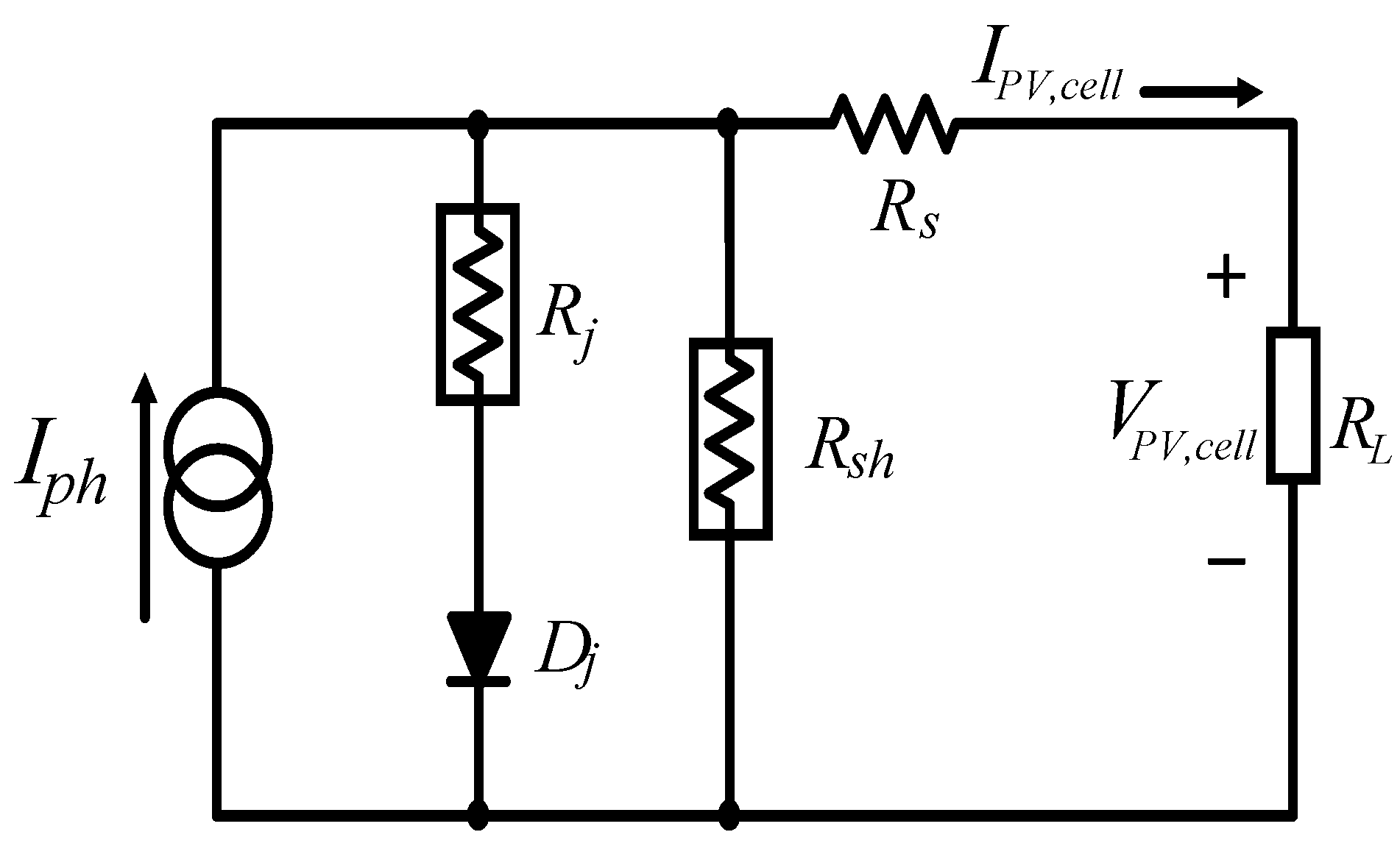
In general, PV arrays are composed of a number of PV modules, which are connected in series and/or in parallel. A PV module is made of a group of PV cells, which are wired to each other and encapsulated in a weatherproof flat container. One side of the module is transparent, allowing sunlight to reach the PV cell. Each PV cell is a p-n junction semiconductor converting solar energy into electricity. An equivalent circuit is shown in
Figure 1, in which
Iph stands for the cell photocurrent source,
Dj represents the p-n junction,
Rj,
Rsh and
Rs are the p-n junction nonlinear impedance, intrinsic shunt resistance and intrinsic series resistance, respectively. The series resistance
Rs is relatively small and the shunt resistance
Rsh is relatively large. Therefore, the equivalent circuit can be simplified by neglecting both resistors.
Figure 1.
An equivalent circuit of a PV cell.
Figure 1.
An equivalent circuit of a PV cell.
From the characteristics of a p-n junction and the equivalent circuit, output current of PV arrays,
IPV, can be described as:
where
VPV is output voltage of PV arrays,
ns is the total number of cells in series,
np stands for the total number of cells in parallel,
q denotes the charges of an electron (1.6 × 10
−19 coulomb),
k is the Boltzmann constant (1.38 × 10
−23 J/°K),
T is temperature of the PV arrays (°K), and
A represents ideality factor of the p-n junction (between 1 and 5) [
16]. In addition,
Isat is the reversed saturation current of the PV cell, which depends on temperature of PV arrays and it can be expressed by the following equation:
where
Tr is the cell reference temperature,
Irr is the corresponding reversed saturation current at
Tr, and
Egap stands for band-gap energy of the semiconductor in the PV cell. In (1), the
Iph varies with irradiation
Si and PV array temperature
T, which can be represented as:
where
Isso is the short-circuit current while reference irradiation is 100 mW/cm
2 and reference temperature is set at
Tr, and
Ki is the temperature coefficient. Based on (1), output power (
PPV) of PV arrays then can be determined as follows:
which reveals that the amount of generated power
PPV varies with irradiation
Si and PV-array temperature
T.
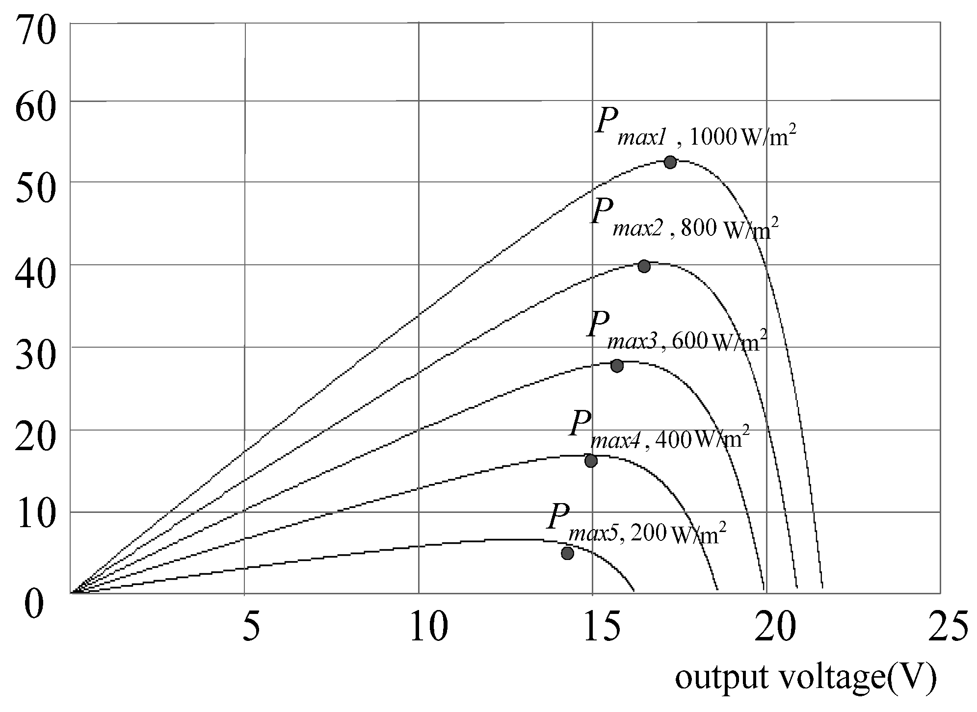
The PV arrays used in this paper are SIEMENS SM55, and the electrical characteristics of each module are listed in
Table 1. By solving equations (1)–(4) and with the values listed in
Table 1, the relationships of
IPV–
VPV and
PPV–
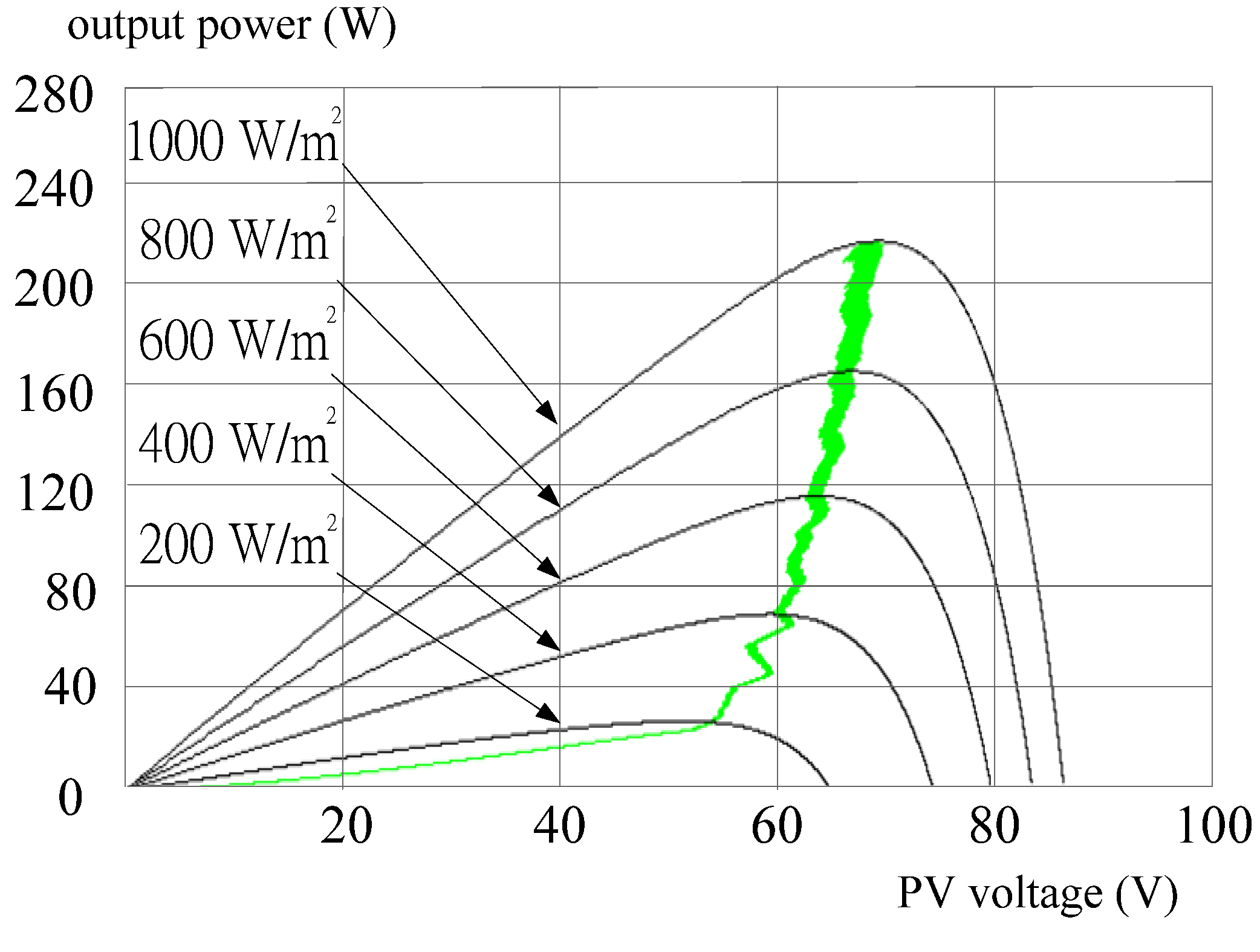
VPV can be plotted. Simulated
PPV–
VPV curves under various irradiations are shown in
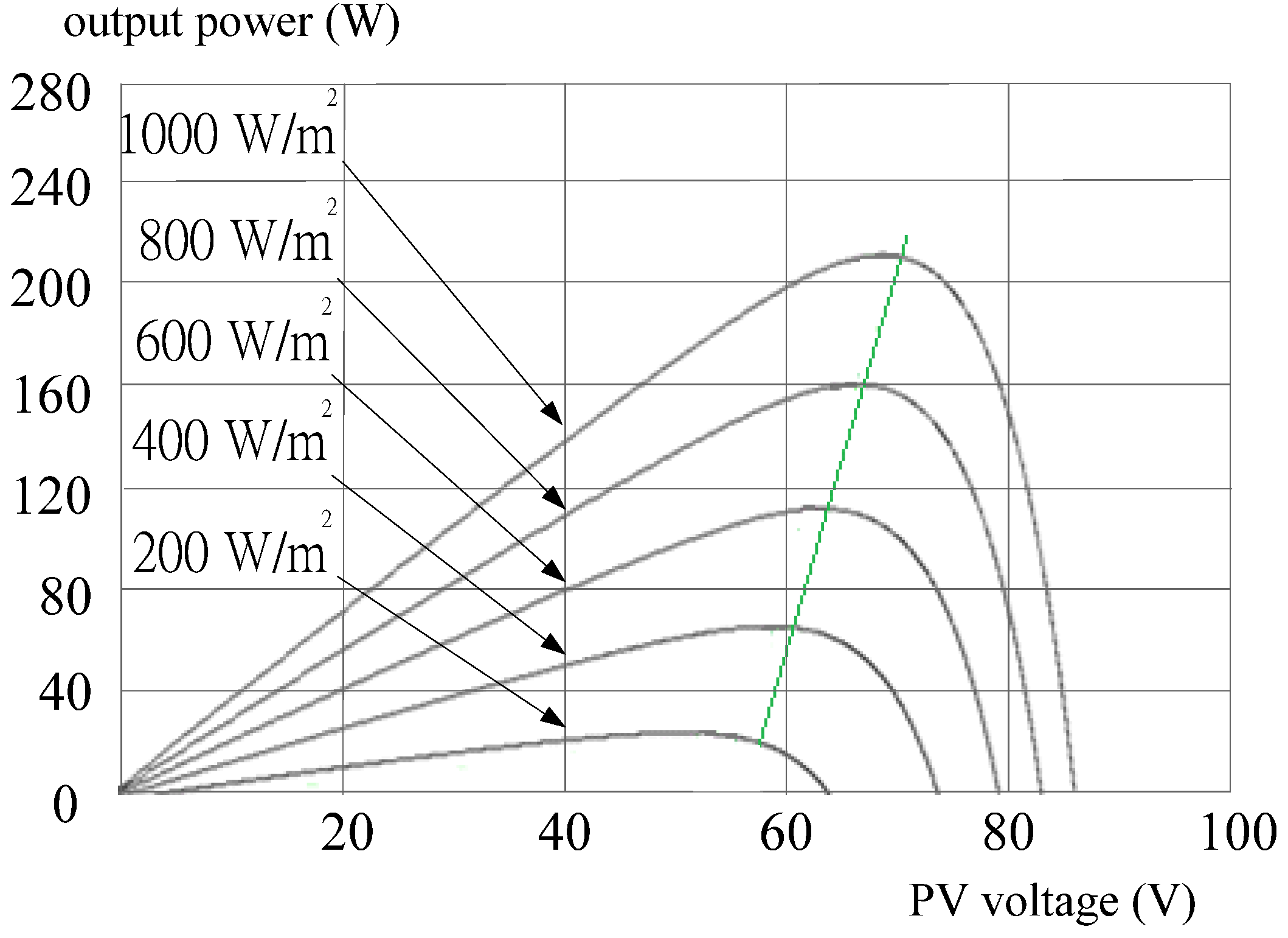
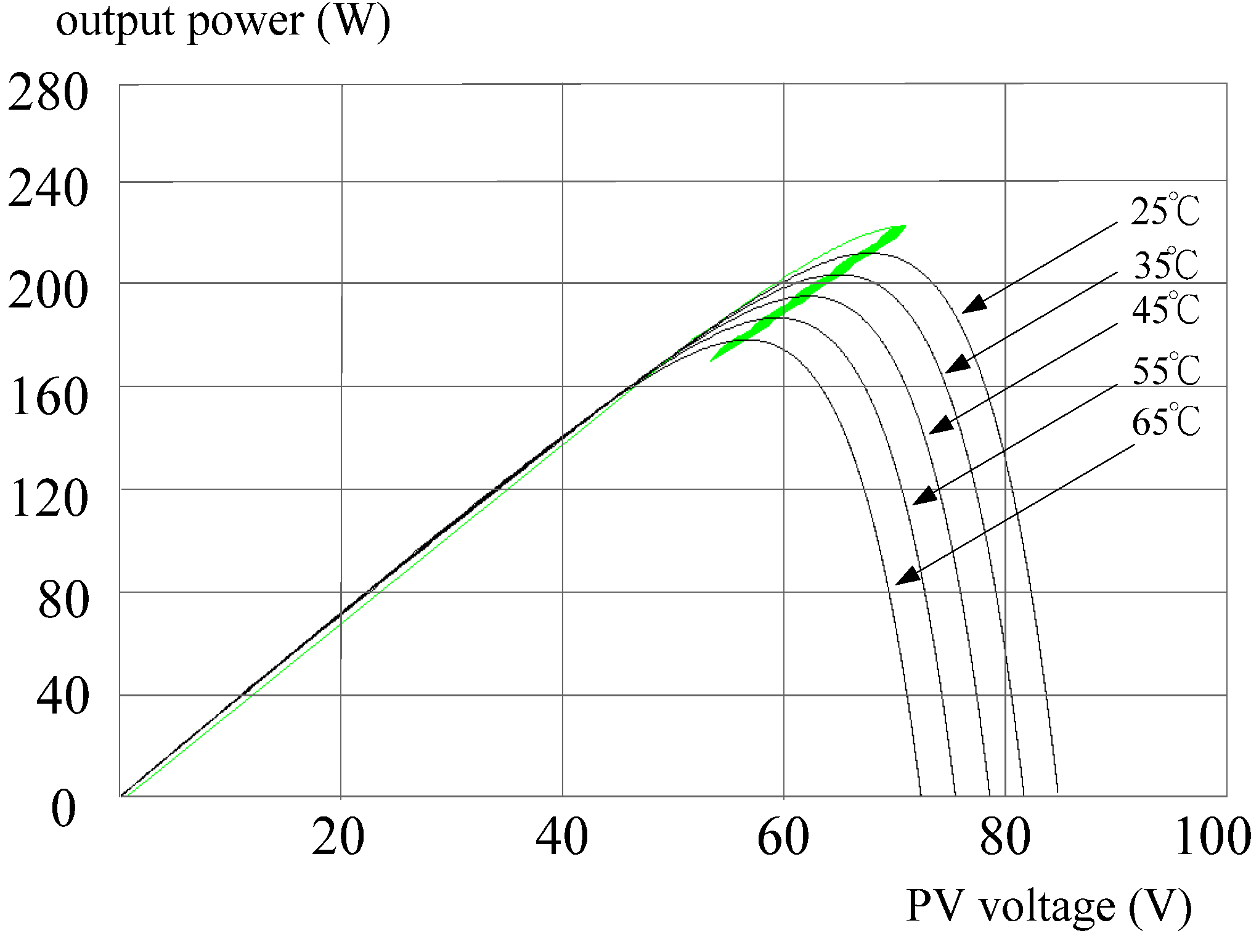
Figure 2 for a fixed module temperature (25 °C). In the case of constant irradiation (1000 W/m
2),
Figure 3 shows the relationship between
PPV and
VPV under various module temperatures.
Table 1.
Electrical characteristics of the used PV module (SIEMENS SM55).
Table 1.
Electrical characteristics of the used PV module (SIEMENS SM55).
| Model | SM55 |
|---|
| Typical peak power (PP) | 55 W |
| Voltage at peak power (VPP) | 17.4 V |
| Current at peak power (IPP) | 3.15 A |
| Short-circuit current (ISC) | 3.45 A |
| Open-circuit voltage (VOC) | 21.7 V |
| Temperature coefficient of open-circuit voltage | −0.077 V/°C |
| Temperature coefficient of short-circuit current (Ki) | 1.2 mA/°C |
Figure 2.
PPV–VPV curves of the PV module with constant temperature (25 °C).
Figure 2.
PPV–VPV curves of the PV module with constant temperature (25 °C).
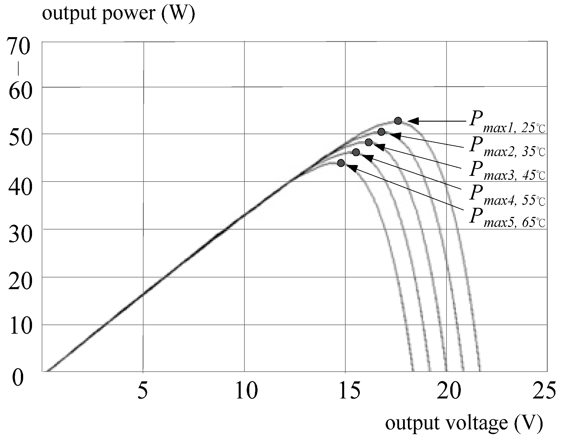
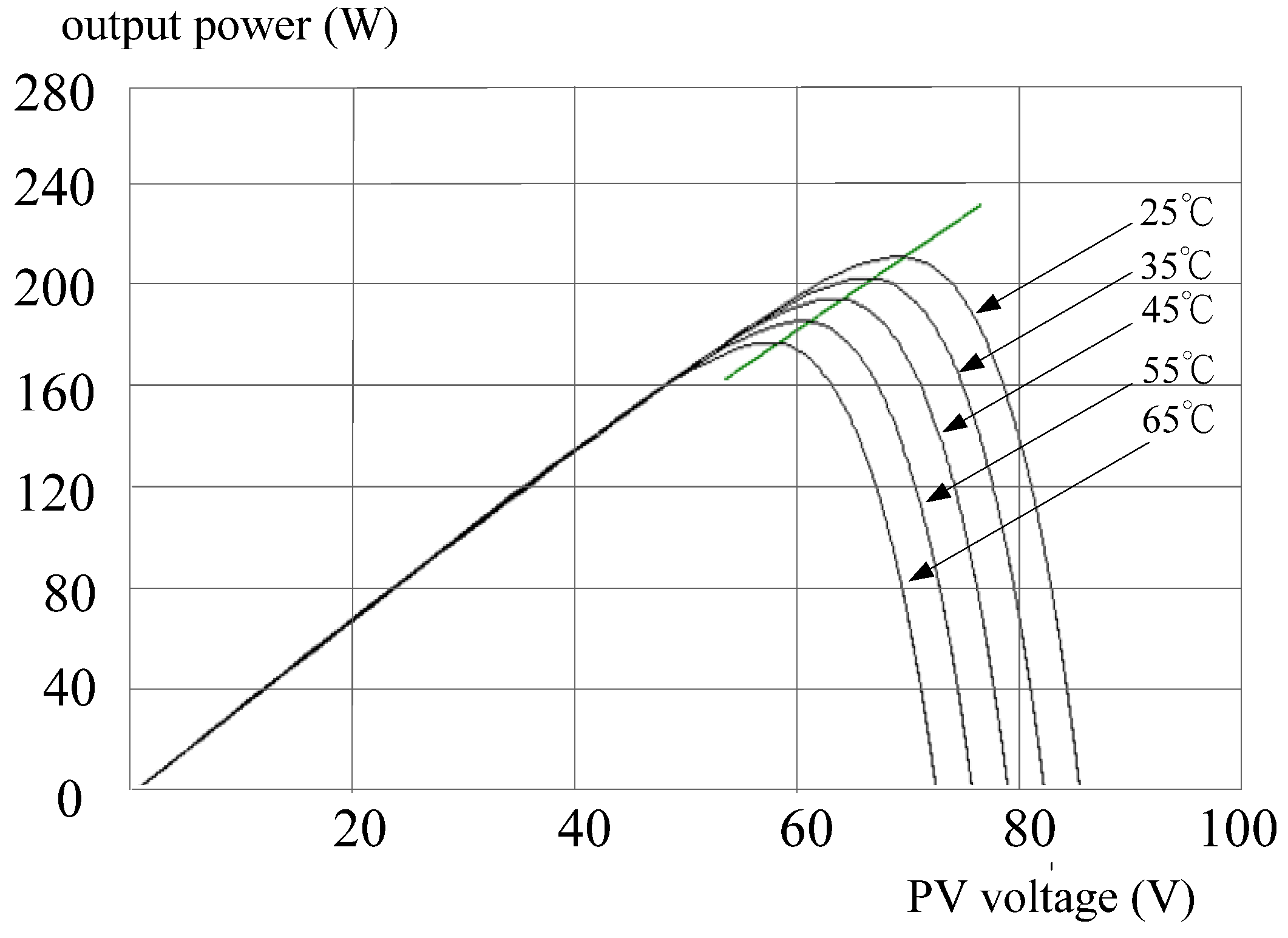
Figure 3.
PPV–VPV curves of the PV module with fixed irradiation (1000 W/m2).
Figure 3.
PPV–VPV curves of the PV module with fixed irradiation (1000 W/m2).
From the above simulations, it is obvious that the two factors, array temperature T and irradiation Si, will affect the generated PV power significantly. To improve system efficiency, an MPPT algorithm has to be adopted to draw maximum power from PV arrays.
3. The Proposed MPPT Algorithm
From
Figure 2 and
Figure 3, we can find that a maximum power point locates at the point of which the derivative of PV output power with respect to terminal voltage equals zero. Therefore, from (3) and (4), the optimal PV terminal voltage
Vref,MPPT to draw maximum power from PV arrays can be obtained:
Suppose that
ns and
np are one. Then, by substituting (5) into (4), the maximum power
PMPPT is expressed as:
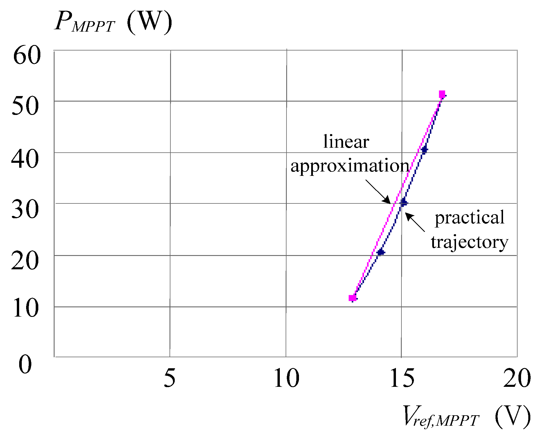
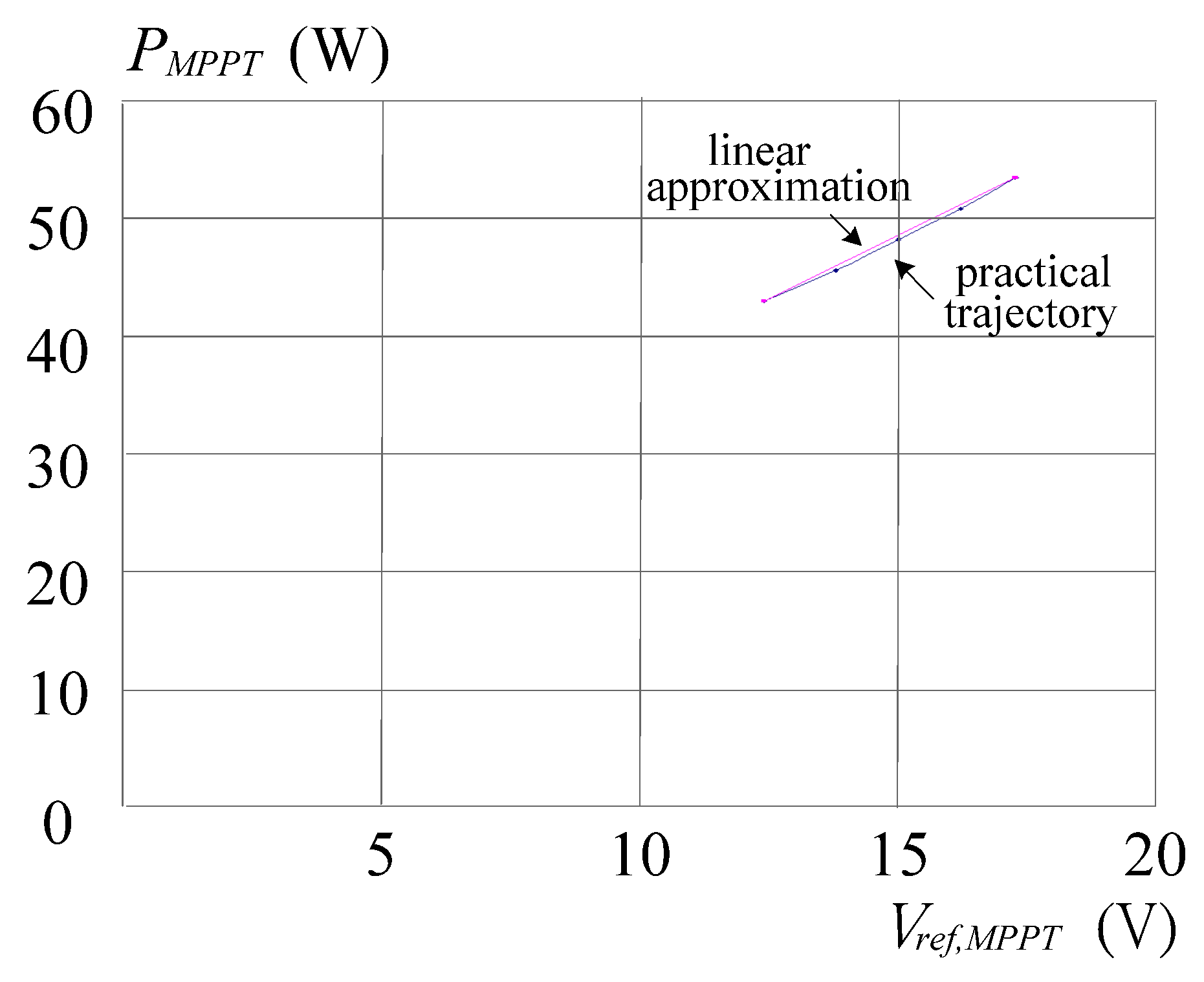
Figure 4 shows the relationship between
PMPPT and
Vref,MPPT under constant module temperature while irradiation varies from 200 to 1000 W/m
2. In the case of fixed irradiation, the trajectory of
PMPPT–
Vref,MPPT with an increase of temperature from 25 to 65 °C is shown in
Figure 5.
Figure 4 and
Figure 5 reveal that
PMPPT is linear to
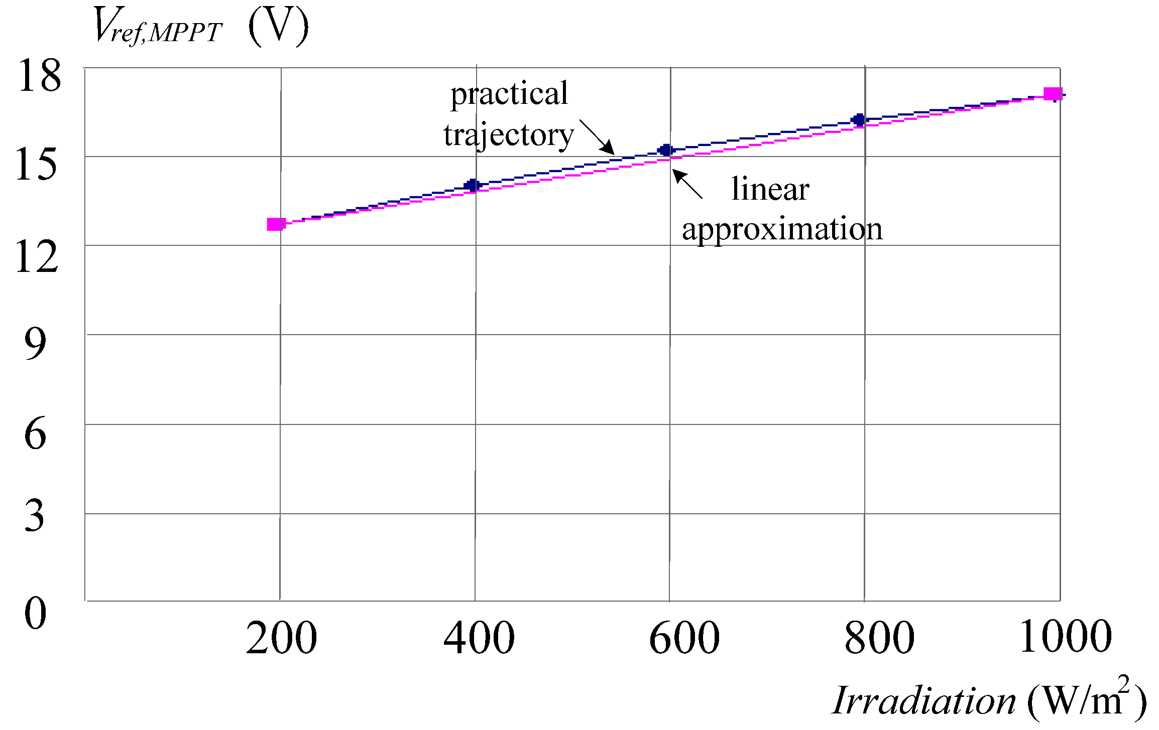
Vref,MPPT approximately. In addition, based on Equation (4), the curves of
Vref,MPPT–T and
Vref,MPPT–
Si are shown in
Figure 6 and
Figure 7, respectively, both of which can be approximated by straight lines. As a result, once a
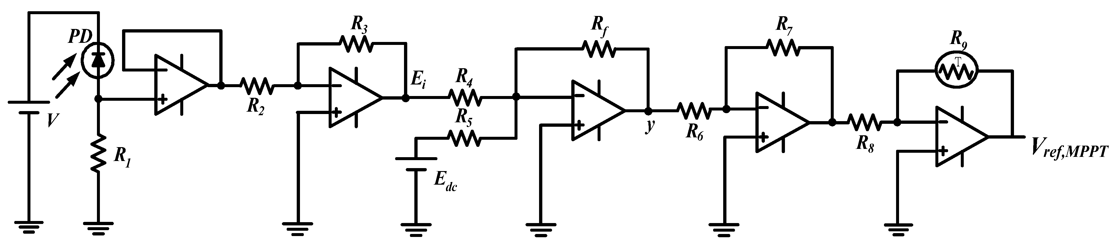
Vref,MPPT is obtained, the MPPT is achieved readily. A corresponding analog circuit to determine
Vref,MPPT is designed and shown in
Figure 8. We choose a photo-diode (PD) for irradiation sensing to realize the first linear approximation shown in
Figure 7 while a negative temperature coefficient of thermal resistor (NTC) is adopted for temperature detecting to practice the second linear approximation shown in
Figure 6. In the DLAA circuit, the potential
Ei is proportional to the magnitude of irradiation and then, the first approximation is determined by:
To consider the influence of temperature, an MPPT voltage obtained by (7) has to be modified, which is approximated by the following second linear relationship. Thus, one can obtain a reference MPPT voltage:
Based on the simple analog circuit, an optimal voltage achieving MPPT feature can be easily obtained.
Figure 4.
The relationship between PMPPT and Vref,MPPT while irradiation increases from 200 to 1000 W/m2.
Figure 4.
The relationship between PMPPT and Vref,MPPT while irradiation increases from 200 to 1000 W/m2.
Figure 5.
The relationship between PMPPT and Vref,MPPT while module temperature increases from 25 to 65 °C.
Figure 5.
The relationship between PMPPT and Vref,MPPT while module temperature increases from 25 to 65 °C.
Figure 6.
The trajectory of Vref, MPPT versus temperature T.
Figure 6.
The trajectory of Vref, MPPT versus temperature T.
Figure 7.
The trajectory of Vref,MPPT versus irradiation Si.
Figure 7.
The trajectory of Vref,MPPT versus irradiation Si.
Figure 8.
The proposed DLAA circuit to determine a voltage command achieving MPPT with analog devices.
Figure 8.
The proposed DLAA circuit to determine a voltage command achieving MPPT with analog devices.
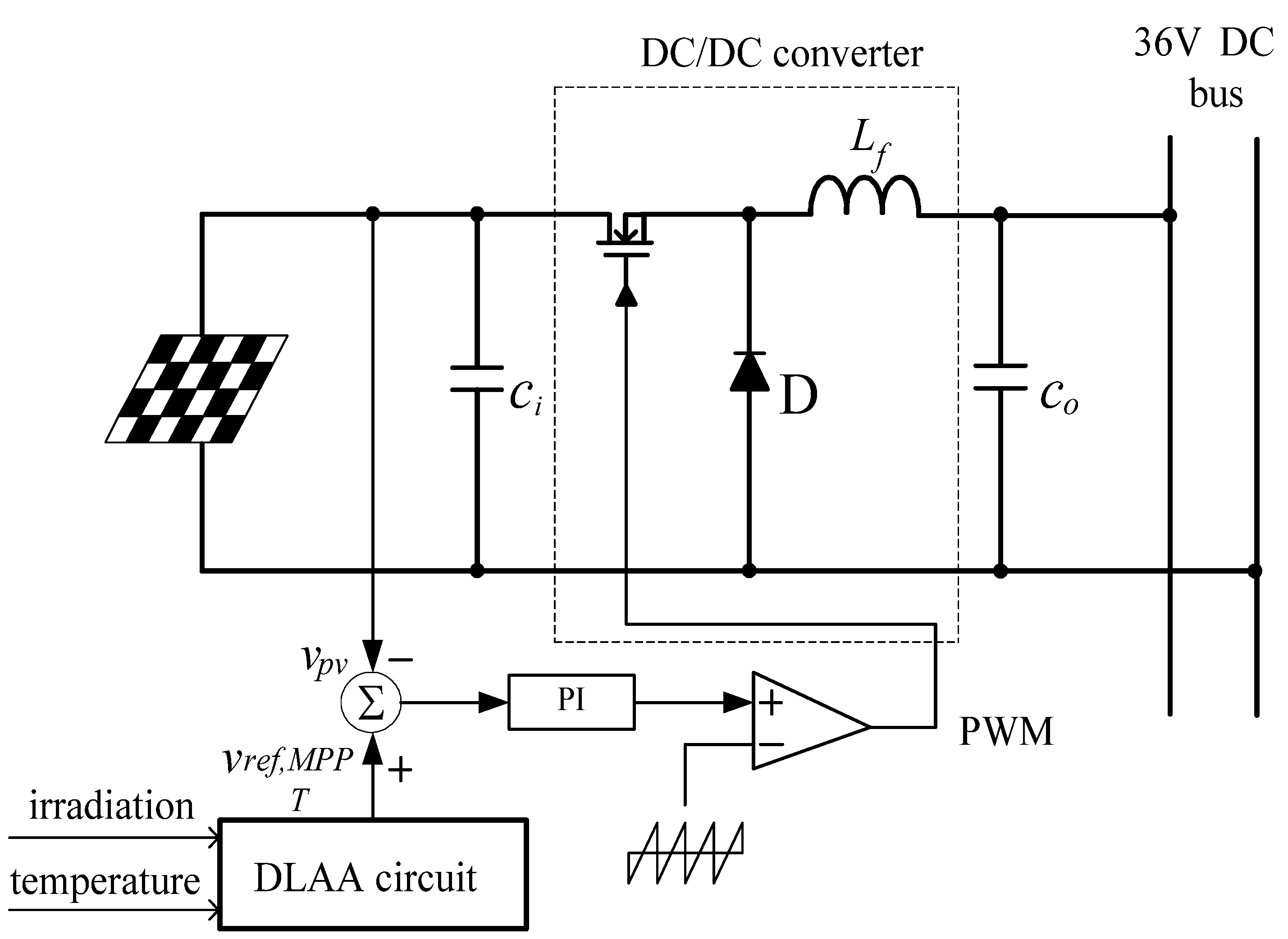
4. Implementation Example
To verify the proposed MPPT algorithm, a PV DC power supply system is constructed, as shown in
Figure 9, which mainly contains PV arrays, a DLAA circuit, and a DC/DC buck converter. The power rating of the converter is 220 W, switching frequency 30 kHz, output voltage 36 V, PV voltage in the range of 45–70 V, and output voltage ripple less than 1%. The converter operates in continuous conduction mode (CCM) while processing power is over 55 W. The minimum inductance
Lf,min are computed as:
in which the
D denotes duty ratio,
Vo is output voltage,
Po stands for output power, and
T expresses switching period. In addition, the minimum output capacitance
Co,min is calculated from:
where
L is the inductance of the converter and Δ
Vo represents the peak-to-peak ripple voltage at the output. Some important parameters of the system are listed as follows:
PV arrays: SIEMENS SM55 (four units in series),
Ci = 100 μF, Co = 100 μF,
Lf = 0.2 mH,
Kp = 0.0295,
Ki = 0.0016,
active power switch: IRF540N, and ultrafast diode: FRF1601CT.
In
Figure 9, the DLAA circuit determines a reference voltage
Vref,MPPT corresponding to an atmospheric condition. The PV output voltage is sensed and compared with the
Vref,MPPT. Through the simple PI controller an appropriate control signal is generated to regulate the PV output voltage so that the DC/DC converter draws maximum power from PV arrays. Then, the DC/DC converter injects the power into DC bus for DC-distribution applications or into utility via a grid-connection DC/AC inverter.
Figure 9.
Illustration of an implementation example which controls PV voltage to fulfill MPPT feature with the proposed DLAA circuit.
Figure 9.
Illustration of an implementation example which controls PV voltage to fulfill MPPT feature with the proposed DLAA circuit.
The MPPT efficiency is calculated by the ratio of the energy drawn by the converter within a defined measuring period
TM to the energy provided by a PV simulator in the MPP. That is:
Theoretical MPPT efficiency of the proposed DLAA can reach 100%. The practical measurement of MPPT efficiency is around 99%.
5. Simulated and Experimental Results
The PV power system mentioned in
Section 4 is simulated and implemented to demonstrate the effectiveness of the proposed approach. In simulation and implementation, both algorithms of the DLAA and the POM are adopted and embedded into the PV power system to fulfill MPPT. With fixed temperature
Figure 10 and
Figure 11 show the simulated MPPT trajectories by the POM and the DLAA, respectively, while
Figure 12 and
Figure 13 show the MPPT results under constant irradiation.
Figure 10.
The MPPT trajectory by the POM under fixed temperature.
Figure 10.
The MPPT trajectory by the POM under fixed temperature.
Figure 11.
The MPPT trajectory by the DLAA under fixed temperature.
Figure 11.
The MPPT trajectory by the DLAA under fixed temperature.
Figure 12.
The MPPT trajectory by the POM under constant irradiation.
Figure 12.
The MPPT trajectory by the POM under constant irradiation.
Figure 13.
MPPT trajectory by the DLAA under constant irradiation.
Figure 13.
MPPT trajectory by the DLAA under constant irradiation.
As irradiation and module temperature increase, the trajectories of MPPT by the POM and the DLAA are shown in
Figure 14 and
Figure 15, in turn.
Figure 14.
MPPT trajectory by the POM while irradiation and temperature increase.
Figure 14.
MPPT trajectory by the POM while irradiation and temperature increase.
Figure 15.
MPPT trajectory by the DALL while irradiation and temperature increase.
Figure 15.
MPPT trajectory by the DALL while irradiation and temperature increase.
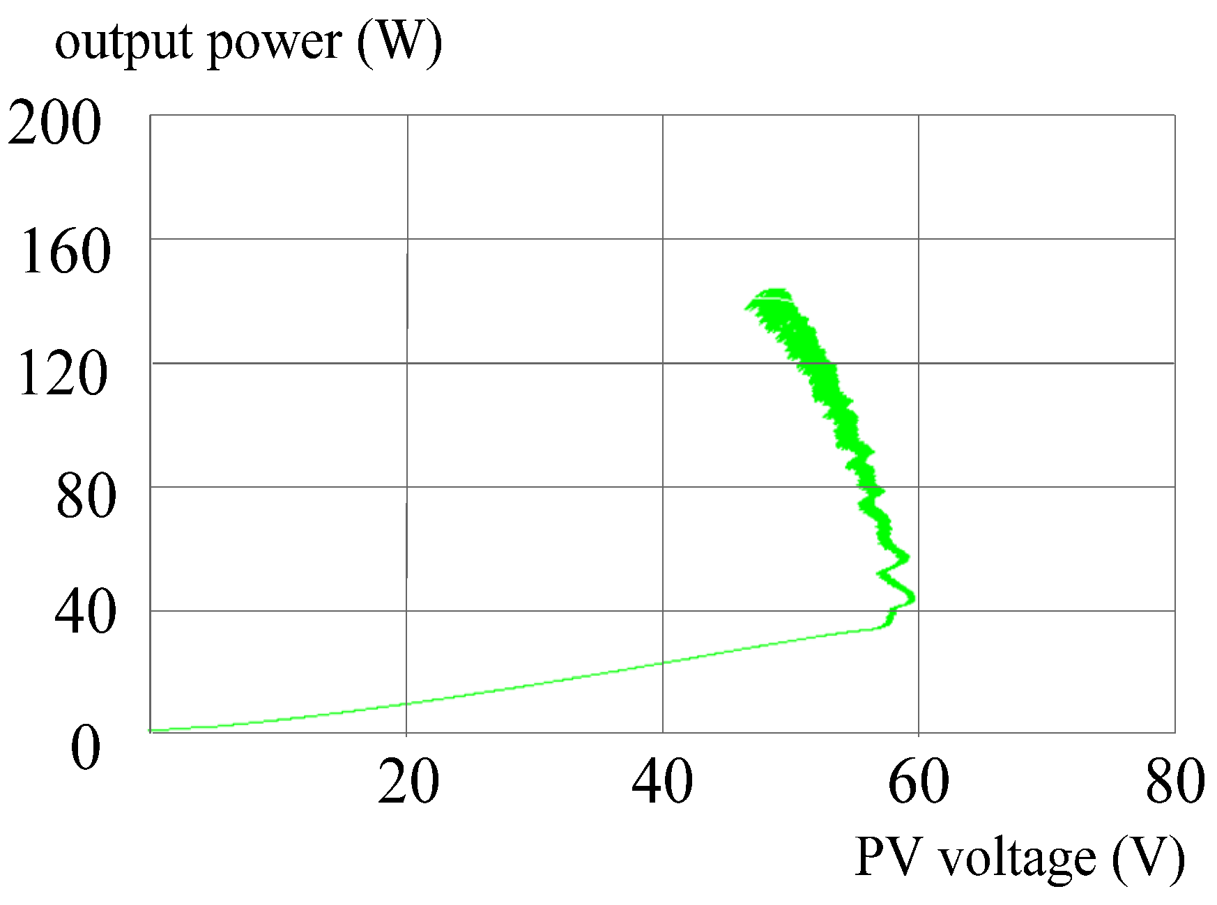
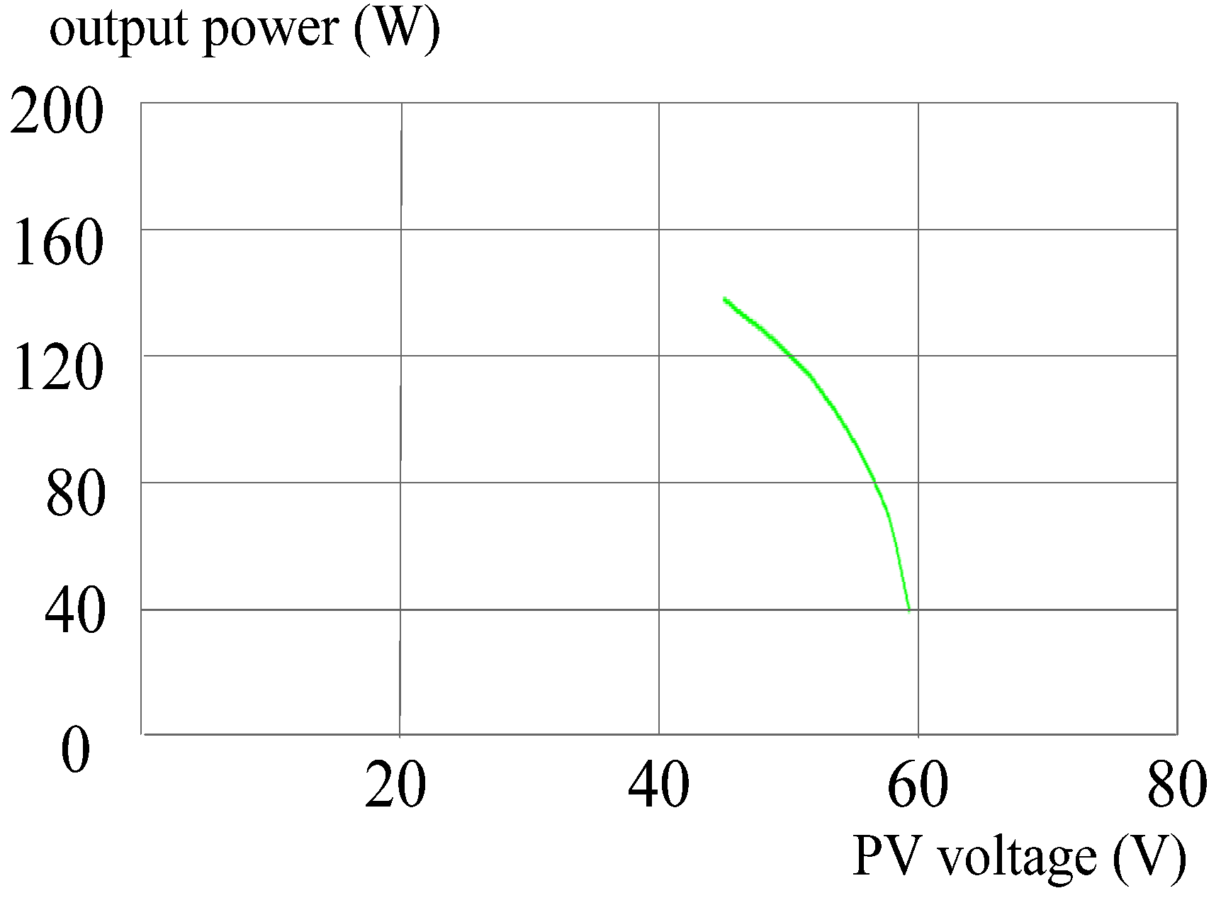
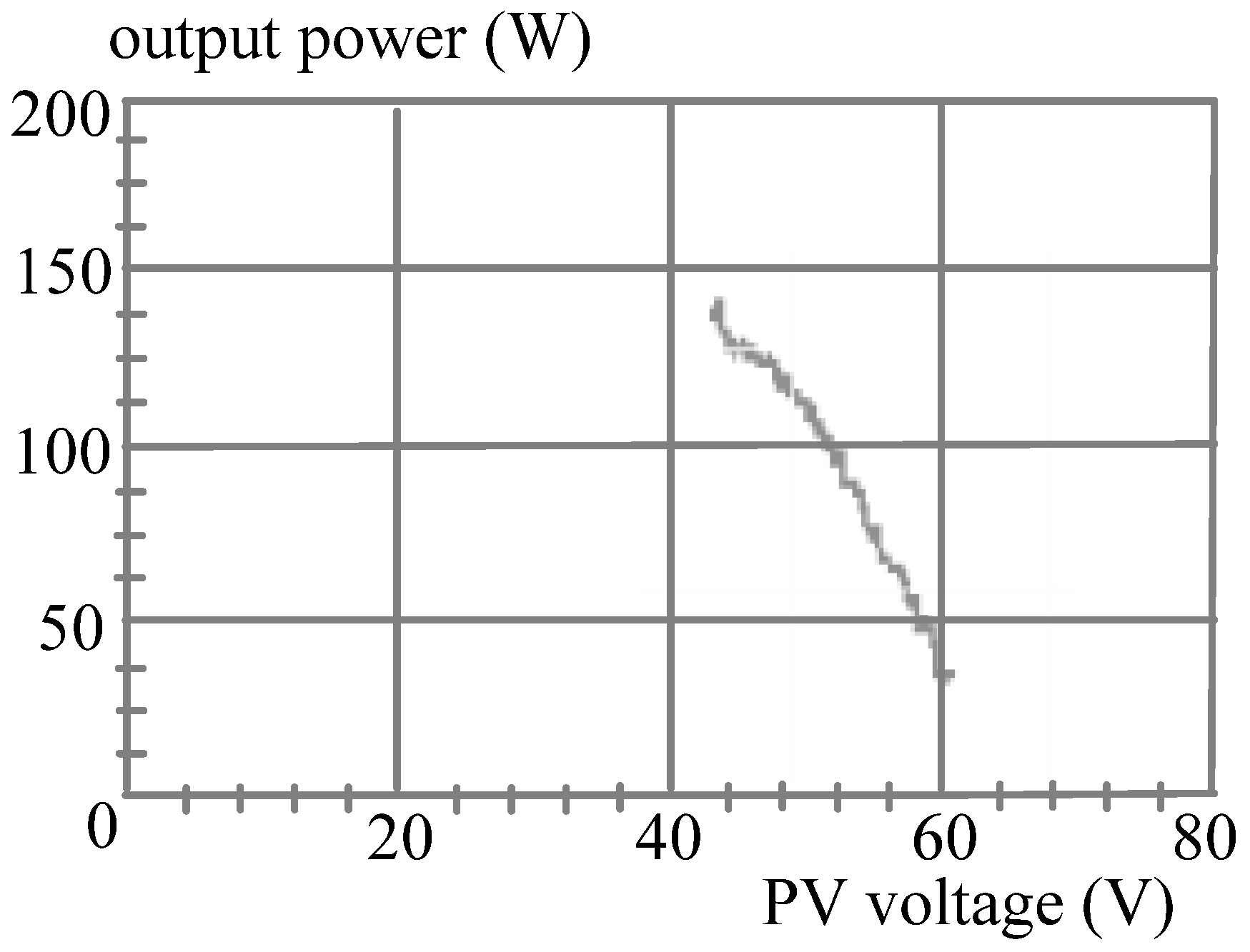
In hardware measurements,
Figure 16 is the practical result of the PV power system with the POM and
Figure 17 shows MPPT trajectory by the DLAA under the variation of atmospheric condition. From
Figure 10,
Figure 11,
Figure 12,
Figure 13,
Figure 14,
Figure 15,
Figure 16 and
Figure 17, it is illustrated that the DLAA can trace MPP effectively and the proposed corresponding circuit is feasible. In addition, a DC/DC converter with the proposed algorithm can obtain better MPPT performance than that with the POM.
Figure 16.
Practical measurement of the PV power system with the POM.
Figure 16.
Practical measurement of the PV power system with the POM.
Figure 17.
Practical measurement of the PV power system with the DLAA.
Figure 17.
Practical measurement of the PV power system with the DLAA.
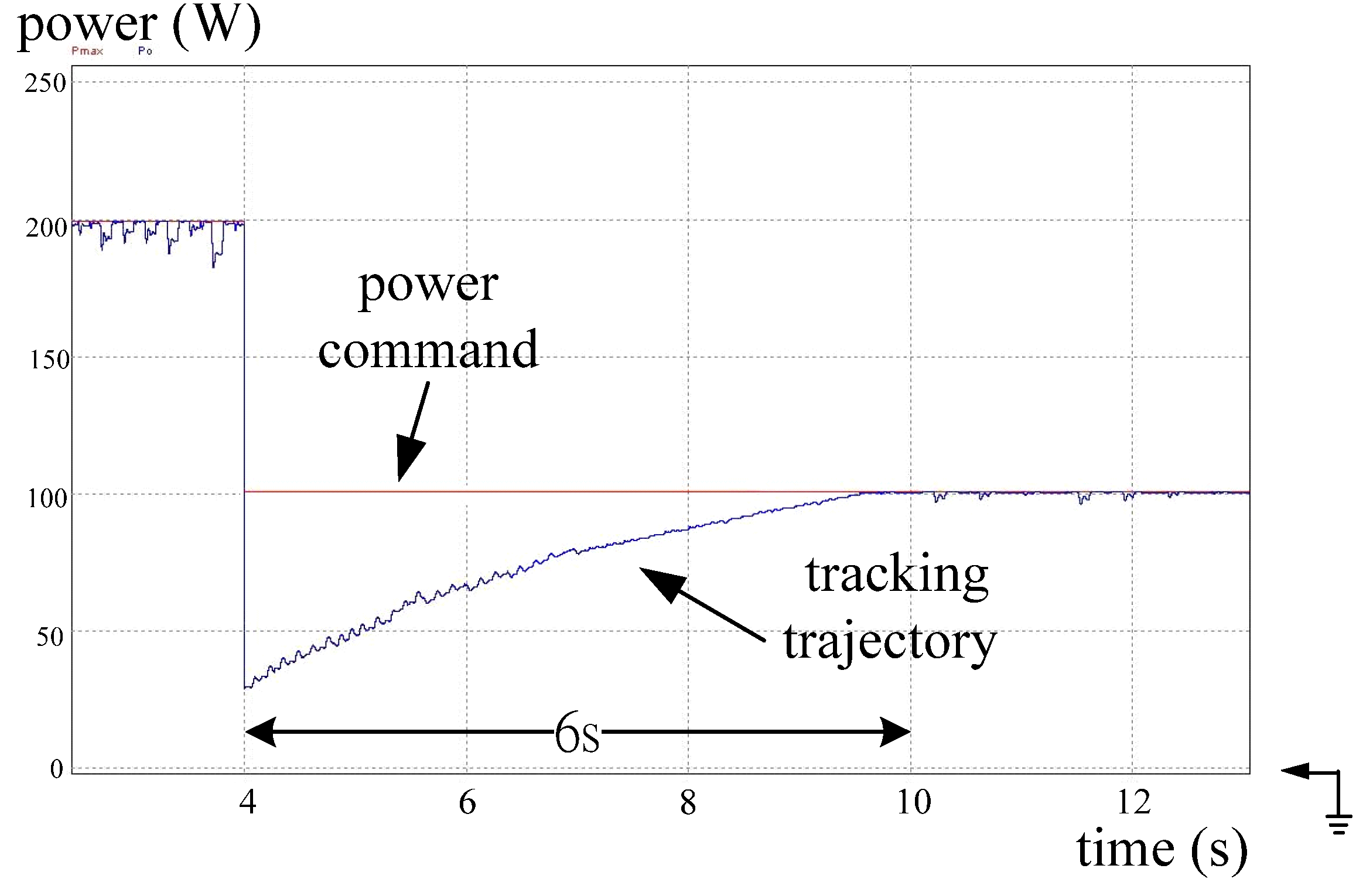
For further comparison between the proposed DLAA and the POM, more simulated results and practical measurements are included in this paper. They are shown in the followings.
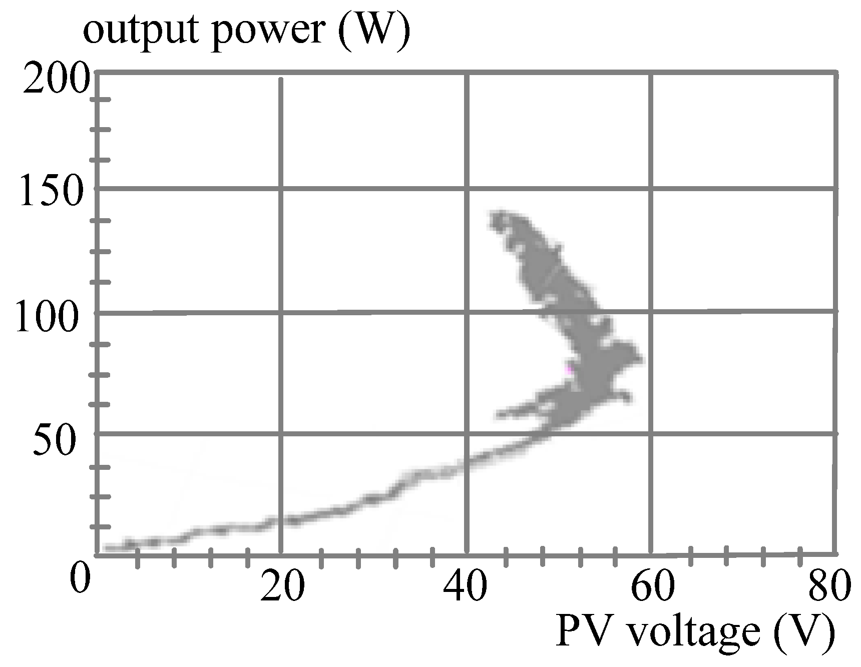
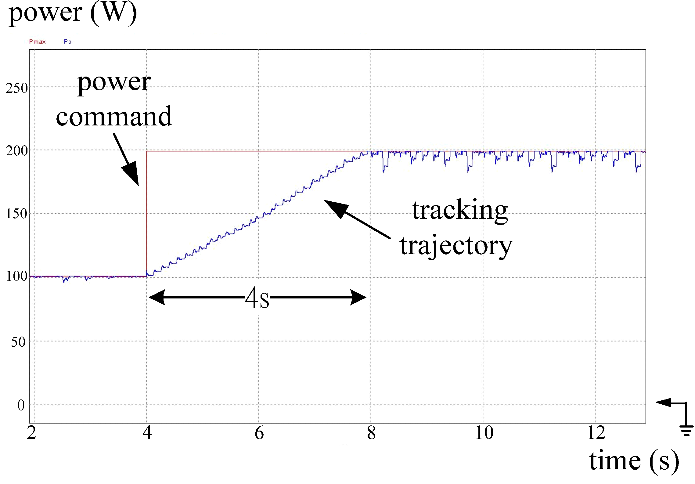
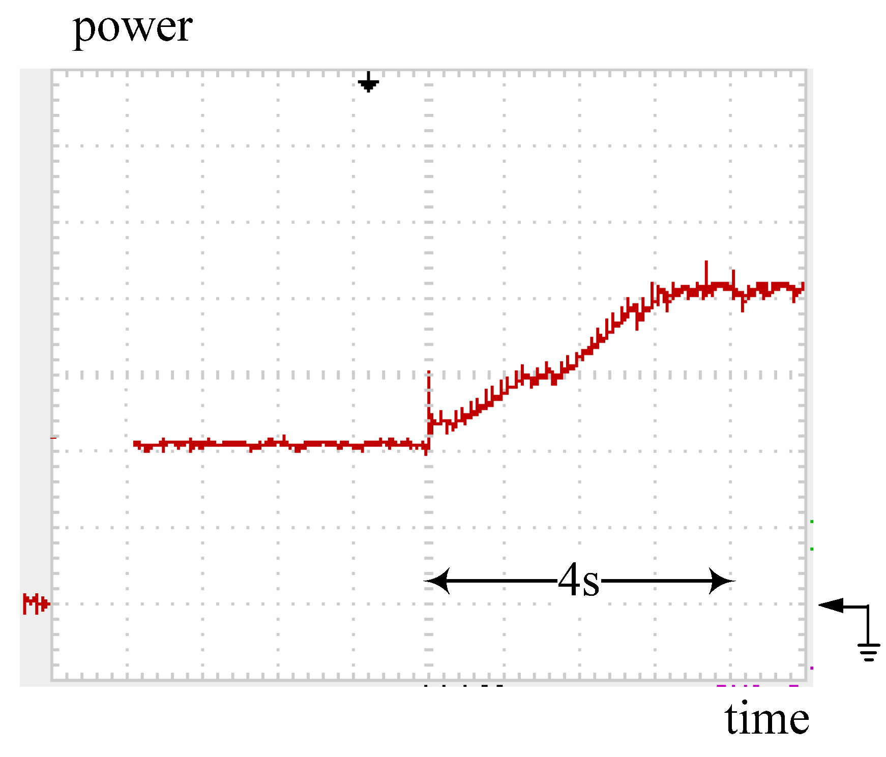
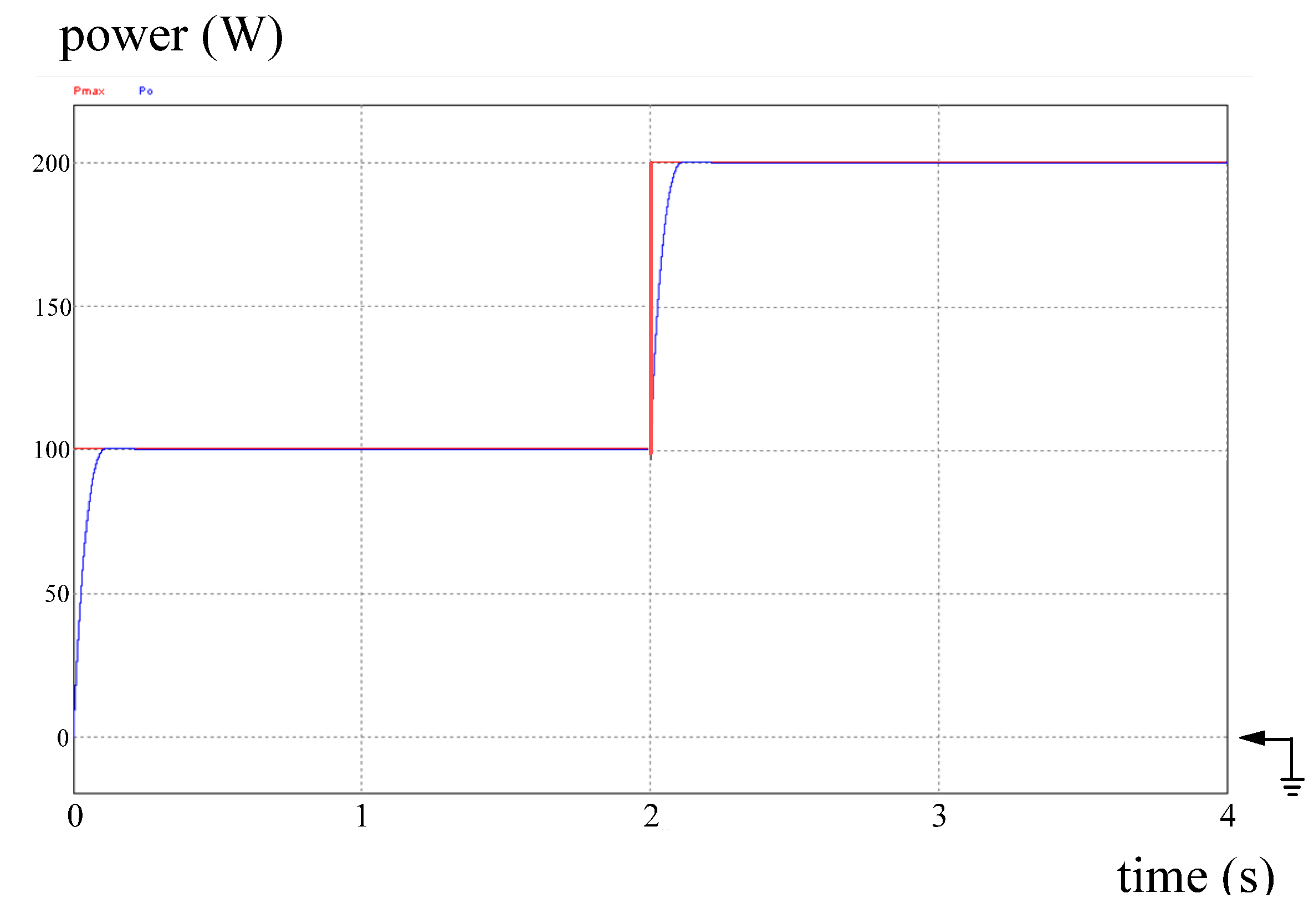
Figure 18 shows the simulated power tracking trajectory of a PV converter with the POM while maximum PV power steps up from 100 W to 200 W. The power tracking trajectory with the proposed DLAA is shown in
Figure 19. From
Figure 18, it can be seen that the transition time is up to 4 s. On the other hand, the proposed DLAA catches up with the new PV power status in around 110 ms. Additionally, the proposed DLAA can effectively prevent operation point from fluctuating.
Figure 18.
Simulated result: tracking trajectory of the converter with the POM while PV power steps up from 100 to 200 W. Note: power: 50 W/div; time: 2 s/div.
Figure 18.
Simulated result: tracking trajectory of the converter with the POM while PV power steps up from 100 to 200 W. Note: power: 50 W/div; time: 2 s/div.
Figure 19.
Simulated result: tracking trajectory of the converter with the DLAA while PV power steps up from 100 to 200 W. Note: power: 50 W/div; time: 1 s/div.
Figure 19.
Simulated result: tracking trajectory of the converter with the DLAA while PV power steps up from 100 to 200 W. Note: power: 50 W/div; time: 1 s/div.
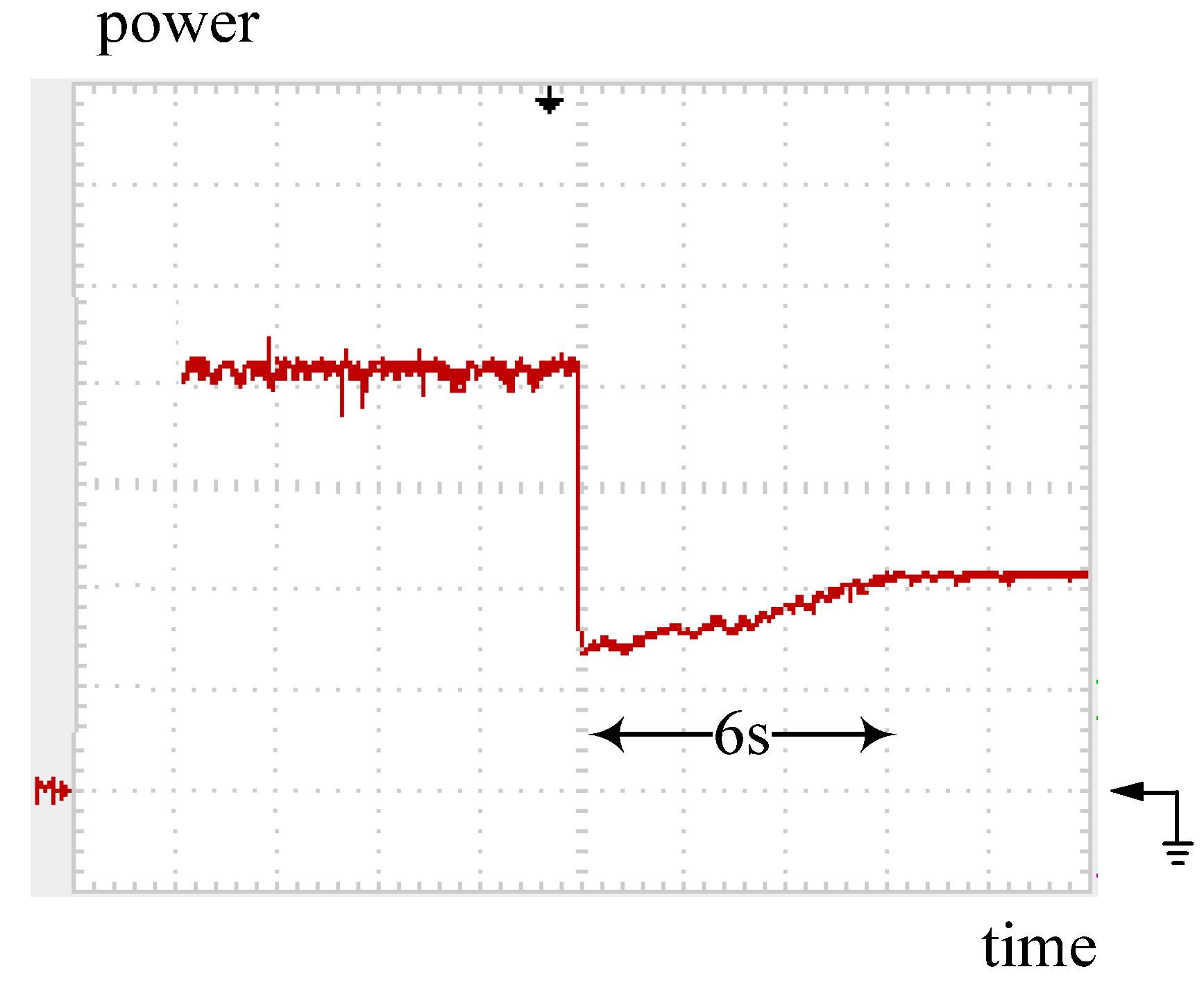
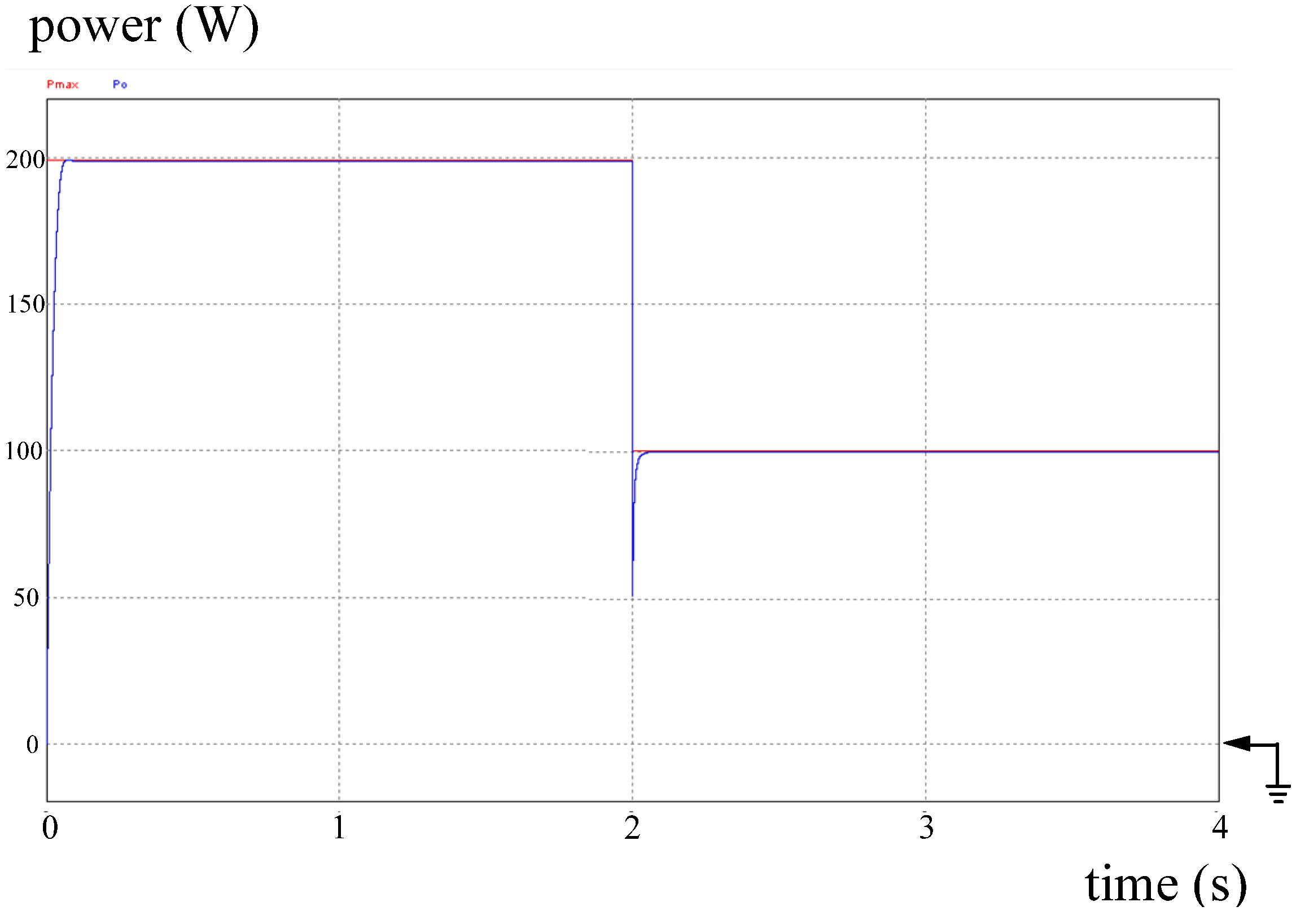
To examine the step-down change,
Figure 20 and
Figure 21 show the simulated results of the PV converter with the POM and with the DLAA, respectively. The transition time is 6 s in
Figure 20 and 50 ms in
Figure 21. In hardware illustration,
Figure 22 is the output power measurement of the converter with the POM in the case of the PV power changing from 100 W to 200 W while
Figure 23 shows the measured result with the DLAA.
Figure 20.
Simulated result: tracking trajectory of the converter with the POM while PV power steps down from 200 to 100 W. Note: power: 50 W/div; time: 2 s/div.
Figure 20.
Simulated result: tracking trajectory of the converter with the POM while PV power steps down from 200 to 100 W. Note: power: 50 W/div; time: 2 s/div.
Figure 21.
Simulated result: tracking trajectory of the converter with the DLAA while PV power steps down from 200 to 100 W. Note: power: 50 W/div; time: 1 s/div.
Figure 21.
Simulated result: tracking trajectory of the converter with the DLAA while PV power steps down from 200 to 100 W. Note: power: 50 W/div; time: 1 s/div.
Figure 22.
Practical measurement: tracking trajectory of the converter with the POM while PV power steps up from 100 to 200 W. Note: power: 50 W/div; time: 1 s/div.
Figure 22.
Practical measurement: tracking trajectory of the converter with the POM while PV power steps up from 100 to 200 W. Note: power: 50 W/div; time: 1 s/div.
Figure 23.
Practical measurement: tracking trajectory of the converter with the DLAA while PV power steps up from 100 to 200 W. Note: power: 50 W/div; time: 0.5 s/div.
Figure 23.
Practical measurement: tracking trajectory of the converter with the DLAA while PV power steps up from 100 to 200 W. Note: power: 50 W/div; time: 0.5 s/div.
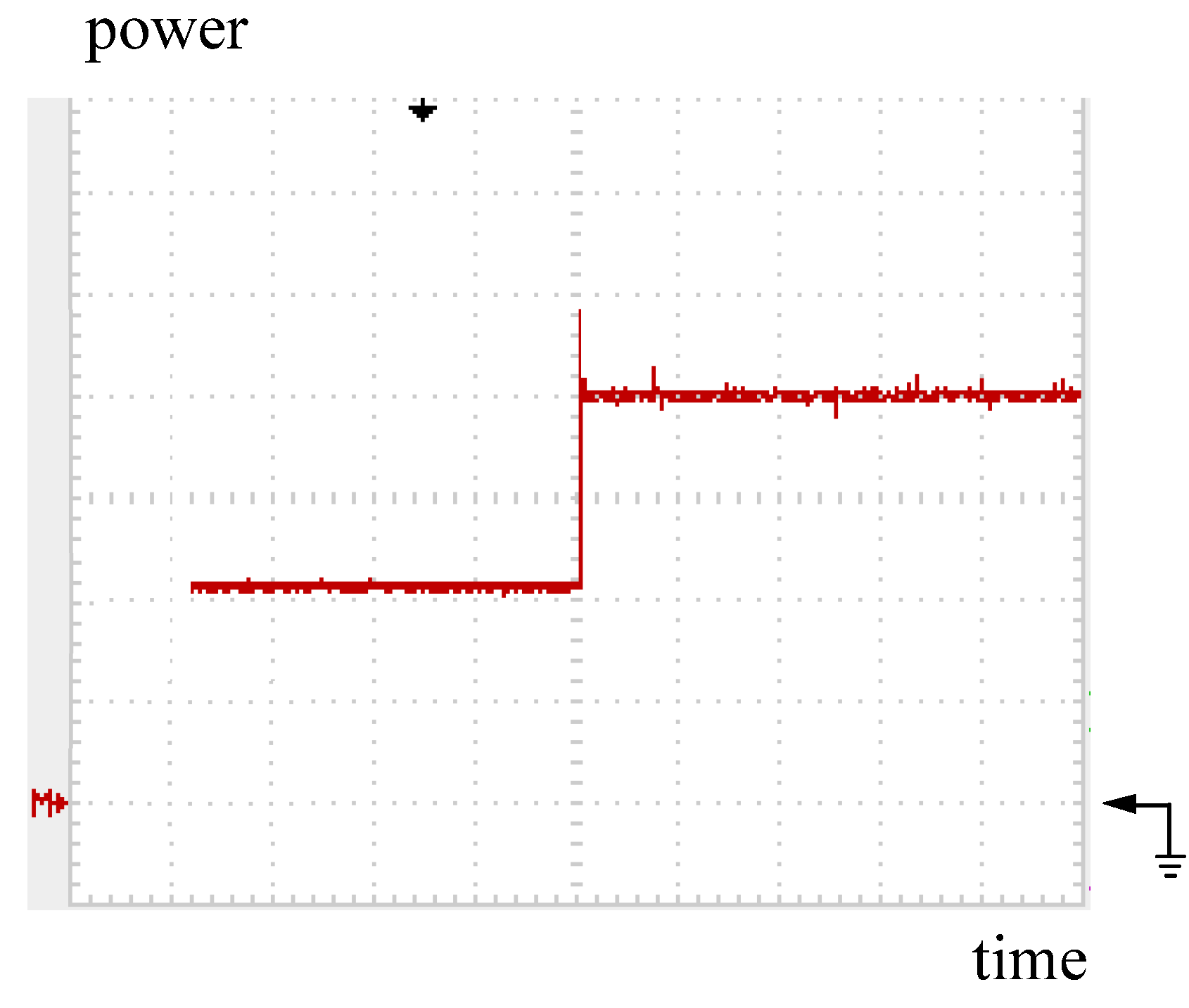
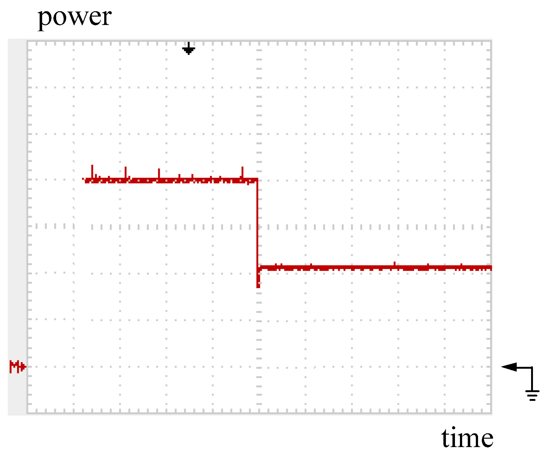
In addition, for 100-to-200 W step-down examination, practical measurements are presented in
Figure 24 and
Figure 25.
Figure 24.
Practical measurement: tracking trajectory of the converter with the POM while PV power steps down from 200 to 100 W. Note: power: 50 W/div; time: 2 s/div.
Figure 24.
Practical measurement: tracking trajectory of the converter with the POM while PV power steps down from 200 to 100 W. Note: power: 50 W/div; time: 2 s/div.
Figure 25.
Practical measurement: tracking trajectory of the converter with the DLAA while PV power steps down from 200 to 100 W. Note: power: 50 W/div; time: 0.5 s/div.
Figure 25.
Practical measurement: tracking trajectory of the converter with the DLAA while PV power steps down from 200 to 100 W. Note: power: 50 W/div; time: 0.5 s/div.


