The Global Inventory of Methane Hydrate in Marine Sediments: A Theoretical Approach

Abstract

The accumulation of methane hydrate in marine sediments is controlled by a number of physical and biogeochemical parameters including the thickness of the gas hydrate stability zone (GHSZ), the solubility of methane in pore fluids, the accumulation of particulate organic carbon at the seafloor, the kinetics of microbial organic matter degradation and methane generation in marine sediments, sediment compaction and the ascent of deep-seated pore fluids and methane gas into the GHSZ. Our present knowledge on these controlling factors is discussed and new estimates of global sediment and methane fluxes are provided applying a transport-reaction model at global scale. The modeling and the data evaluation yield improved and better constrained estimates of the global pore volume within the modern GHSZ (≥44 × 10¹⁵ m³), the Holocene POC accumulation rate at the seabed (~1.4 × 10¹⁴ g yr⁻¹), the global rate of microbial methane production in the deep biosphere (4−25 × 10¹² g C yr⁻¹) and the inventory of methane hydrates in marine sediments (≥455 Gt of methane-bound carbon).

1. Introduction

The global abundance of methane hydrate in marine sediments is still poorly constrained. Estimates are based on extrapolation of field data [1,2] and geochemical transport-reaction modeling [3,4,5,6]. They range over three orders of magnitude (500–55,700 Gt of C) and a clearly constrained consensus value has not emerged over the past decades. This is a major draw-back for gas hydrate research since the resource potential and the possible impact of methane hydrates on past and future climate change cannot be evaluated without a better constrained estimate of global methane hydrate abundance. Models and observations clearly show that methane hydrate formation is basically controlled by the following key parameters: (1) accumulation of particulate organic carbon at the seafloor; (2) kinetics of microbial organic matter degradation and methane generation in marine sediments; (3) thickness of the gas hydrate stability zone (GHSZ); (4) solubility of methane in pore fluids within the GHSZ; (5) sediment compaction; (6) ascent of deep-seated pore fluids and methane gas into the GHSZ. In the following, we present a comprehensive review on the key parameters listed above and identify major knowledge gaps. Subsequently, a geochemical transport-reaction model is applied to investigate the effects of the key parameters on gas hydrate accumulation in marine sediments on a quantitative basis. The model is finally used to constrain the global gas hydrate inventory in marine sediments.

2. Accumulation of Particulate Organic Carbon at the Seafloor

Methane production and methane hydrate formation are fueled by the accumulation of particulate organic carbon (POC) at the seabed. The mass accumulation rate of sediments (MAR in g cm⁻² yr⁻¹) and the POC accumulation rate (A_POC in g cm⁻² yr⁻¹) are calculated as:

$$\begin{array}{l}MAR={\rho }_{\text{S}}\cdot \left(1-\Phi \right)\cdot w A_{POC}=\frac{PO{C}_0}{100}\cdot MAR\end{array}$$

(1)

where POC₀ is the concentration of particulate organic carbon in surface sediments (in wt.%), ρ_S is the density of dry solids (in g cm⁻³), Ф is porosity and w is burial velocity (in cm yr⁻¹). The density of dry solids in continental margin sediments varies from 2.65 g cm⁻³ for quartz to 2.1–2.76 g cm⁻³ for different types of clay minerals. Here, we adopt ρ_S = 2.5 g cm⁻³ as mean density of dry solids at continental margins [6]. The porosity of bioturbated surface sediments (0–10 cm sediment depth) usually falls into a range of 0.7–0.9 at most continental margins. Thus, a mean value of Ф = 0.8 is applied in the following to convert burial velocities of surface sediments into mass accumulation rates [6].

2.1. Holocene POC Accumulation Rates

POC concentrations in Holocene surface sediments have been measured at several thousand sites covering most depositional areas at the seabed [7,8]. The available data have been compiled and evaluated to produce a global map of POC concentrations in marine surface sediments (Figure 1).

Figure 1. Concentration of particulate organic carbon (POC) in Holocene surface sediments [7,8]. The color coding indicates POC values in wt.%. Regions of the seafloor where data are not available are shown in white.

Figure 1. Concentration of particulate organic carbon (POC) in Holocene surface sediments [7,8]. The color coding indicates POC values in wt.%. Regions of the seafloor where data are not available are shown in white.

For some parts of the global seafloor POC concentrations are not available (see white areas in Figure 1). In the following, we assume a POC value of 1 wt.% for these areas. Burial velocities of Holocene surface sediments have also been determined at several hundred locations [6]. The published data clearly show that burial velocities are high on the continental shelf and decrease with increasing water depth. Most of the sediments accumulating at the seabed are derived from the continents. Moreover, the solid remains of marine plankton (carbonate, biogenic opal) are deposited at the deep-sea floor as pelagic sediments. The global accumulation rate of sediments at the modern seafloor amounts to about 19.6 × 10¹⁵ g yr⁻¹. This number has been derived considering the transport of riverine, eolian and ice-rafted sediments to the ocean, the accumulation of neritic carbonates at the continental shelf and the accumulation of pelagic sediments at the deep-sea floor [6]. The depth-distribution of sediment accumulation and the global accumulation rate can be used to constrain parameter values of a logistics equation defining the burial velocity as function of water depth [6]:

$$w=\frac{w_1}{1+{\left(\frac{z}{z_1}\right)}^{c_1}}+\frac{w_2}{1+{\left(\frac{z}{z_2}\right)}^{c_2}}$$

(2)

with w₁ = 0.117 cm yr⁻¹, w₂ = 0.006 cm yr⁻¹, z₁ = 200 m, z₂ = 4000 m, c₁ = 3, c₂ = 10, and z in m. Equation (2) yields a global sediment accumulation of 19.6 × 10¹⁵ g yr⁻¹ for Ф = 0.8 and ρ_S = 2.5 g cm⁻³ when applied to the global bathymetric data set given by Menard and Smith [9]. The equation predicts that most of the global sedimentation takes place on the continental shelf (14.1 × 10¹⁵ g yr⁻¹ at 0–200 m water depth). These estimates are consistent with other data recently presented by Baturin [10]. Baturin derived a total sedimentation rate of 18.9 × 10¹⁵ g yr⁻¹ with a shelf and upper slope contribution of 13.6 × 10¹⁵ g yr⁻¹. Sediments accumulating at shallow water depths (<200 m) cannot contribute to gas hydrate accumulation since marine methane hydrates are only formed at significantly higher pressures i.e., water depths. During the Holocene, the accumulation of methane hydrates is thus severely limited by the continental shelf acting as a trap for the continental sediment input.

Holocene POC accumulation rates are calculated at global scale applying Equations (1,2) with Ф = 0.8 and ρ_S = 2.5 g cm⁻³ and the POC concentrations shown in Figure 1. The resulting global map shows high A_POC values at the shelf of productive continental margins where POC is rapidly buried in terrigenous sediments (Figure 2). Burial velocities vary over several orders of magnitude from less than 1 cm kyr⁻¹ in Pacific deep-sea basins to more than 100 cm kyr⁻¹ on the continental shelf while most of the POC concentrations fall into the range of 0.1 to 1 wt.%. The A_POC variability is thus mainly induced by the strong contrast in burial velocity between pelagic and continental margin settings. The global POC accumulation rate in Holocene surface sediments calculated from the distribution shown in Figure 2 amounts to 1.37 × 10¹⁴ g yr⁻¹. Since continental margins are the main locus for sediment accumulation, 88% of the global POC accumulation occurs within 500 km distance from the coastline (Figure 2). Our new estimate of Holocene POC accumulation (1.37 × 10¹⁴ g yr⁻¹) is very close to a previous estimate (1.40 × 10¹⁴ g yr⁻¹) given by Baturin [10] even though Baturin’s global rate is based on an independent data set and modeling approach. This surprising conformity strongly supports the validity of the new approach presented by Burwicz et al. [6].

Figure 2. Accumulation rate of POC in Holocene surface sediments in g m⁻² yr⁻¹ at 0.5° × 0.5° spatial resolution.

Figure 2. Accumulation rate of POC in Holocene surface sediments in g m⁻² yr⁻¹ at 0.5° × 0.5° spatial resolution.

2.2. Quaternary POC Accumulation Rates

Most of the methane produced in marine sediments does not originate from Holocene surface sediments. The thickness of these Holocene deposits rarely exceeds 10 m while the gas hydrate stability zone extends several hundred meters into the sub-surface. Thus, mean POC accumulation rates averaged over a period of several million years are more appropriate for the prediction of hydrate accumulation than Holocene accumulation rates. During the Holocene, most riverine particles are deposited on the continental shelf because the shelf is not at isostatic equilibrium with the present sea level but is still affected by the much lower glacial sea level stand [11]. The sea level was 120 m below its present value during the last glacial maximum [12] reducing the water-covered shelf and marginal sea areas by more than 50% [9,13,14]. Under glacial conditions, the anomalous Holocene shelf accumulation rate may have been diminished by an order of magnitude [15] shifting the focus of sedimentation from the shelf to the continental rise and slope. Moreover, the transport of ice-rafted material and the deposition of eolian dust were strongly enhanced further increasing the accumulation rates at the margin seafloor [16]. Hydrates only accumulate in margin sediments deposited at more than 200 m water depth at the continental slope and rise. The mean Quaternary sedimentation rate in this environment is certainly much higher than the Holocene value. The sediment accumulation at 200–3000 m water depth would rise by a factor of 5 if most of the Holocene shelf sedimentation was shifted to larger water depth under glacial conditions as proposed by Hay [15]. Quaternary burial velocities were thus calculated increasing the sedimentation rate at the continental slope and rise (>200 m water depth) at the expanse of shelf deposits [6]. The global sediment accumulation rate was maintained while the slope and rise burial velocities were enhanced by a factor of 5 over a 500 km wide zone around the continental margins [6]. This 500 km zone includes the continental slope and a major portion of the continental rise. The resulting burial velocities were then applied to calculate Quaternary POC accumulation rates. These calculations were based on the Holocene POC distribution map (Figure 1) since mean Quaternary POC concentrations are not available at global scale. The error involved in the map of the Quaternary POC accumulation (Figure 3) thus exceeds the error of the corresponding Holocene distribution (Figure 2). Nevertheless, methane generation and gas hydrate accumulation in the modern ocean are controlled by the Quaternary mean values (Figure 3) rather than the anomalous Holocene accumulation rates (Figure 2). The global POC accumulation rate for Quaternary surface sediments calculated from the distribution shown in Figure 3 amounts to 1.55 × 10¹⁴ g yr⁻¹. In the Quaternary reconstruction, 89.5% of the global POC accumulation occurs within a distant of 500 km from the coastline. The accumulation is, however, shifted from the shelf to the continental rise and slope.

Figure 3. Accumulation rate of POC in Quaternary sediments (in g m⁻² yr⁻¹).

Figure 3. Accumulation rate of POC in Quaternary sediments (in g m⁻² yr⁻¹).

2.3. Cenozoic–Cretaceous POC Accumulation Rates

Global accumulation rates of terrigenous sediments at the seafloor reconstructed over the last 150 Myr [17] show a strong increase towards the Quaternary induced by high rates of continental erosion (Figure 4). Quaternary erosion was accelerated by the waxing and waning of continental ice shields, rapid sea-level change and intense mountain building in the Himalayas and Tibetan High Plateau. Global rates of POC accumulation at the seafloor were reconstructed using the δ¹³C record of marine carbonates [17]. They feature a maximum during the Quaternary induced by high rates of sediment accumulation (Figure 4). However, the contrast to the previous periods is not as strong as observed for terrigenous sedimentation. It thus seems that average concentrations of POC in marine sediments were higher in the geological past [Equation (1)]. Very high POC concentrations may have prevailed prior to the Paleocene-Eocene Thermal Maximum (PETM) at 55.5 Myr. These high concentrations may have favored the built-up of a large marine gas hydrate inventory which was possibly destabilized during the PETM to induce the large negative δ¹³C excursion observed in the geological record [18].

Figure 4. Accumulation of POC and terrigenous sediments over the last 150 Myr. The solid line shows the global marine POC accumulation rate normalized to the Quaternary value while the dotted line gives the global rate of terrigenous sedimentation at the seafloor normalized to the Quaternary [17]. The Paleocene-Eocene Thermal Maximum (PETM, at 55.5 Myr) is indicated by the vertical arrow.

Figure 4. Accumulation of POC and terrigenous sediments over the last 150 Myr. The solid line shows the global marine POC accumulation rate normalized to the Quaternary value while the dotted line gives the global rate of terrigenous sedimentation at the seafloor normalized to the Quaternary [17]. The Paleocene-Eocene Thermal Maximum (PETM, at 55.5 Myr) is indicated by the vertical arrow.

3. Microbial Degradation of Organic Matter and Methane Formation in Marine Sediments

Stable carbon isotope data show that methane hydrates are usually formed from biogenic methane produced by the anaerobic degradation of organic matter in the deep marine biosphere. It is thus important to understand the mechanisms and kinetics of organic matter degradation and microbial methane formation in the marine subsurface. Organic matter deposited at the seabed is degraded by microorganisms and other benthic biota using oxygen as terminal electron acceptor. The remaining organic matter is degraded by anaerobic bacteria and archaea using dissolved nitrate and manganese (+IV) and iron (+III) minerals as oxidizing agents [19]. These additional electron acceptors are usually consumed within the bioturbated surface layer (0–10 cm sediment depth). Field data show that only a small fraction of the POC raining to the seafloor is buried below 10 cm depth [20]. The data reveal a marked contrast between fine-grained continental margin and deep-sea sediments [21]. While at continental margins about 10% of the POC raining to the seabed is conserved and buried below 10 cm sediment depth, this fraction is reduced to about 1% at the deep-sea floor [20]. Due to the very low preservation of POC in open ocean environments, gas hydrates are usually not found in pelagic sediments but only at continental margins where a significant POC fraction is buried and therefore available for microbial methane formation in the deep subsurface.

POC buried below the bioturbated surface layer is further degraded by anaerobic bacteria and archaea using dissolved sulfate as electron acceptor:

C(H₂O) + ½ SO₄²⁻ → HCO₃⁻ + ½ H₂S

(3)

where C(H₂O) represents sedimentary POC.

Microbial methane production and accumulation starts below the depth of sulfate penetration. Several steps are needed before methane is finally produced as stable end product of anaerobic microbial POC degradation. In a first step, biogenic polymers are hydrolyzed and converted into monomers. These monomers (sugars, amino acids, lipids, etc.) are then fermented into CO₂, H₂ and a number of organic acids. Methane is finally formed by methanogenic microorganisms converting CO₂ and H₂ into methane [22]:

CO₂ + 4 H₂ → CH₄ + 2 H₂O

(4)

The stoichiometry of the overall process of organic matter degradation and methanogenesis is given by the following reaction:

2 C(H₂O) → CH₄ + CO₂

(5)

Equation (5) does not imply that methane is directly formed by POC degradation. It rather defines the substrate and the final products. The intermediate steps including fermentation and CO₂ reduction with H₂ are included in the overall stoichiometry [23].

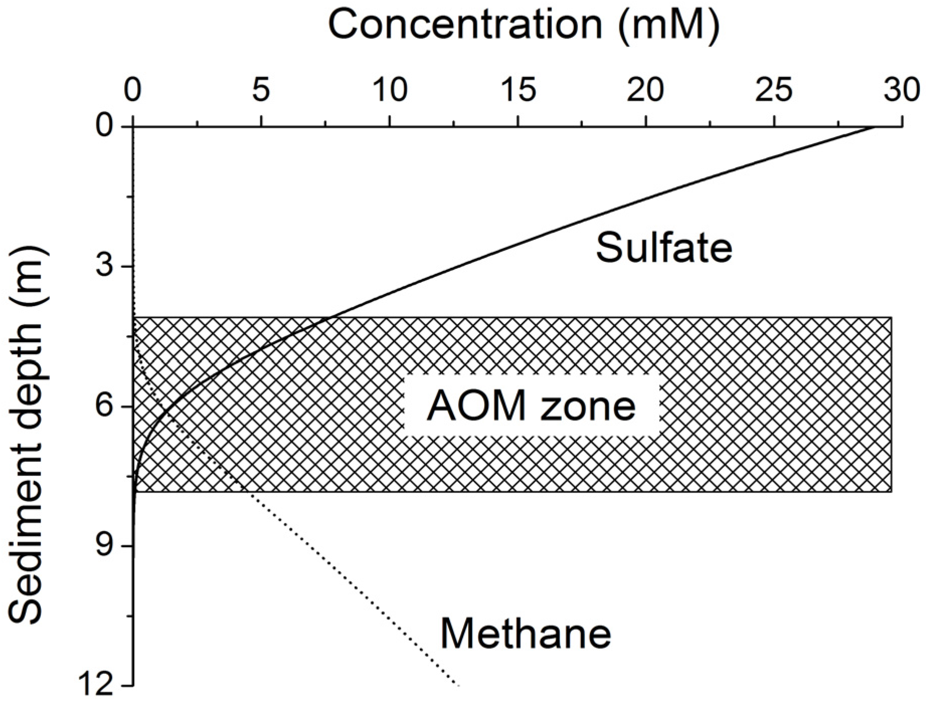
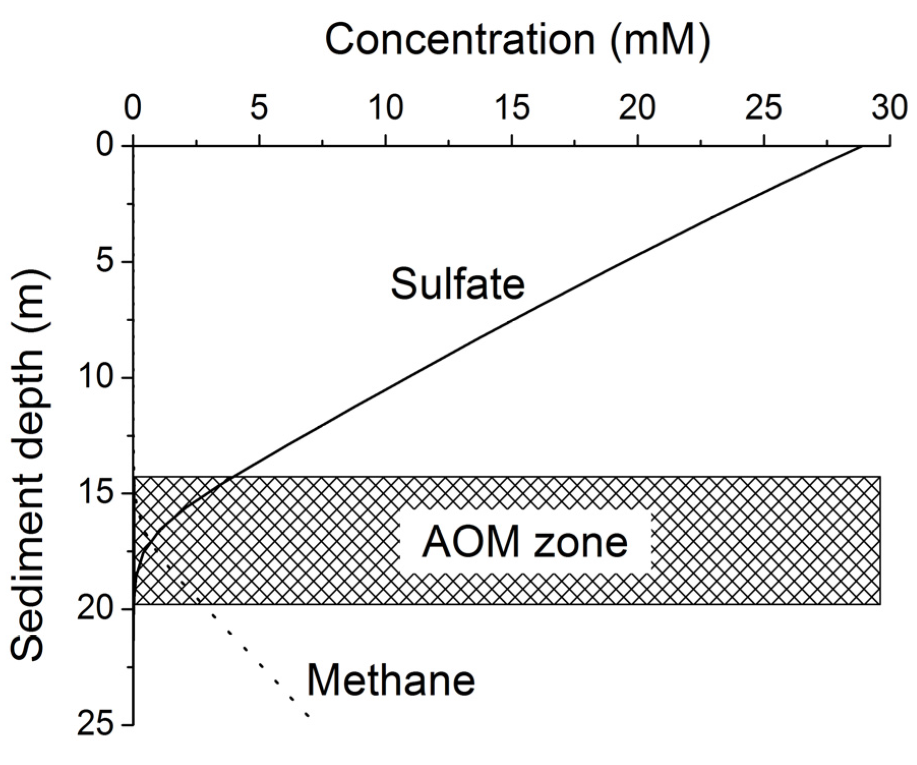
Methane formed at depth is transported upwards into the sulfate-methane transition zone (SMTZ) via molecular diffusion and advection. Within this zone, methane is oxidized by consortia of bacteria and archaea using sulfate as terminal electron acceptor [24]. The overall stoichiometry of anaerobic oxidation of methane (AOM) within the SMTZ is given by:

CH₄ + SO₄²⁻ → HCO₃⁻ + HS⁻ + H₂O

(6)

Considering this complex network of microbial processes, the key questions that need to be answered to estimate the global rate of methane formation may be formulated as: How much POC is reaching the methanogenic zone and how much of that POC can be microbially converted into methane? To answer these questions not only the POC burial rates but also the down-core changes in POC reactivity need to be defined. Since more than three decades marine geochemists and microbiologists have observed that the POC reactivity decreases strongly with sediment age and depth. In his classical paper on POC degradation kinetics in marine sediments Middelburg showed that the down-core decrease in POC reactivity can be represented by the following equation [25]:

$$k_{age}=0.16\cdot {\left(ag{e}_0+age\right)}^{-0.95}$$

(7)

where k_age is the age-dependent reactivity (in yr⁻¹) and age₀ is the initial age of POC (in yr). The rate of POC degradation (R_POC in g C g⁻¹ yr⁻¹) is calculated as:

$$R_{POC}=-\frac{\partial C_{POC}}{\partial t}=k_{age}\cdot C_{POC}$$

(8)

where C_POC is the POC concentration (in g C per g of dry sediment). The equation was calibrated by a large number of rate measurements showing that the reactivity of POC decreases by 10 orders of magnitude going from fresh marine plankton to POC buried in deep-sea sediments. More recently, ODP drilling confirmed the presence of living microorganisms in pelagic and terrigenous sediments down to the underlying oceanic crust [26,27,28,29]. The number of prokaryotic cells (bacteria and archaea) decreases from more than 10⁸ cm⁻³ in the upper few meter of the sediment column to less than 10⁶ cm⁻³ at depth [26,30]. The logarithmic down-core decrease in cell numbers and the microbial POC degradation rates in the deep subsurface are broadly consistent with the rates predicted by the Middelburg model [27,31,32].

The main uncertainty of the Middleburg model is associated with the initial age parameter (age₀) defined as the average age of POC buried below the bioturbated zone. Initial ages of 300–30,000 yrs were applied to reproduce the pore water profiles in sediment cores retrieved from the Sakhalin slope [23]. An even larger range of 800–180,000 yrs was needed to reproduce pore water profiles measured in ODP sediment cores [33]. These large ranges probably reflect the ambient variability in burial velocity, the deposition of refractory organic matter and the possible loss of surface sediments during core retrieval [23]. The largest initial ages were observed at Blake Ridge where drift sediments are deposited containing pre-aged organic matter of terrigenous and marine origin [23,33].

Equations (7,8) can be combined and solved to estimate the POC loss within the sulfate reduction zone and thereby the input of POC into the methanogenic zone. The fraction of POC reaching the methanogenic zone results in:

$$f_{\text{MI}}=\exp \left(3.2\cdot ag{e}_0{}^{1/20}-3.2\cdot {\left(t_{\exp }+ag{e}_0\right)}^{1/20}\right)$$

(9)

where t_exp is the sulfate exposure time and f_MI is the concentration of POC in sediments reaching the methanogenic zone divided by the POC concentration in sediments buried below the bioturbated zone at 0.1 m depth. The sulfate exposure time depends on sulfate penetration depth (z_S in m) and burial velocity (w in m yr⁻¹):

$$t_{\exp }=\frac{z_{\text{S}}-0.1}{w}$$

(10)

Burial velocities at the deep-sea floor typically range from 0.1 to 10 cm kyr⁻¹ [Equation (2)] while sulfate penetrates usually more than 100 m into pelagic sediment. A compilation of sulfate penetration depths in open ocean sediments confirmed that sulfate is usually not fully depleted in these pelagic deposits [32]. This observation is partly explained by the deep penetration of dissolved oxygen into pelagic sediments [29] and the delivery of sulfate through the base of the sediment column via sulfate-rich fluids circulating through the underlying oceanic crust. Deep-sea sediments are thus typically exposed to sulfate over their entire life span (up to ~150 Myr). Microbial rate measurements and pore water profiles obtained in pelagic sediments revealed that methanogenesis may occur already within the sulfate-bearing sediment horizons [27]. Methane produced by this process is, however, consumed within the sulfate-bearing zone via AOM. Methane concentrations in pelagic sediments are therefore several orders of magnitude lower than the ambient saturation value with respect to methane hydrate [34]. Due to this strong undersaturation of pore fluids, methane hydrates have never been documented in pelagic sediments.

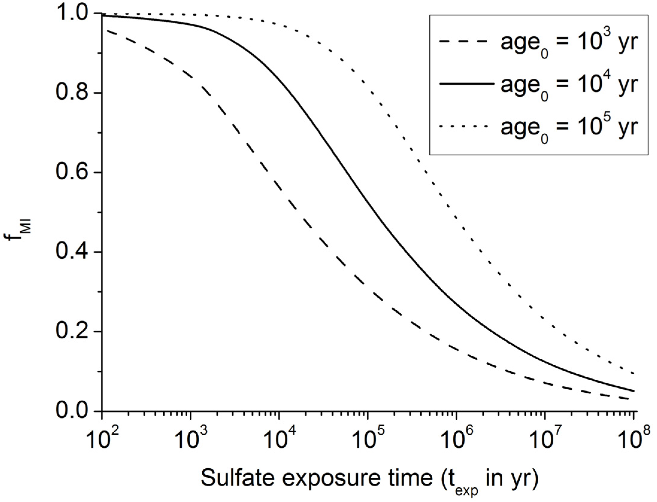
In most continental margin settings, sulfate dissolved in ambient pore fluids is completely consumed at 10–100 m sediment depth [32,35]. The sulfate exposure time results as t_exp = 10⁴–10⁶ yr for burial velocities of 10–100 cm kyr⁻¹. Thus, about 30–90% of the buried POC is reaching the methanogenic zone in continental margin sediments (Figure 5). The microbial degradation of POC delivered to the sulfate-free methanogenic zone may lead to the accumulation of methane in pore fluids and to the formation of methane hydrates pending on the rate of methane formation and the local pressure and temperature conditions.

Figure 5. Fraction of buried POC entering the methanogenic zone (f_MI) as calculated from Equation (9) for initial ages of 1000 yrs, 10,000 yrs, and 100,000 yrs.

Figure 5. Fraction of buried POC entering the methanogenic zone (f_MI) as calculated from Equation (9) for initial ages of 1000 yrs, 10,000 yrs, and 100,000 yrs.

Dissolved sulfate profiles often show an almost linear decrease with sediment depth suggesting that only a minor sulfate fraction is used for POC degradation while most of the sulfate is consumed via AOM in the underlying sulfate-methane transition zone [36,37]. Equation (9) implies that only 10% of the POC buried in continental margin sediments is consumed via microbial sulfate reduction where pre-aged organic matter (age₀ = 10⁵ yr) is deposited at the seabed (Figure 5). It is thus likely that linear sulfate profiles are induced by the deposition of old POC at the seabed. Terrestrial POC delivered to the margins by continental erosion is a likely source for this pre-aged material. However, sulfate profiles with significant curvature documenting strong sulfate depletion via anaerobic POC degradation are also commonly observed [23]. They probably reflect the deposition of young marine organic matter since Equation (9) implies that up to 80% of this young POC (age₀ = 10³ yr) is consumed via microbial sulfate reduction (Figure 5).

The kinetics of microbial methane formation in marine sediments was studied in detail by Wallmann et al. [23]. Evaluating pore water and sediment data from the Sakhalin Slope and the Blake Ridge, the authors showed that the rate of methane formation within the methanogenic zone (R_CH4 in g of methane carbon g⁻¹ yr⁻¹) can be calculated as:

$$R_{{\text{CH}}_{\text{4}}}=-0.5\frac{d{C}_{POC}}{dt}=\frac{0.5K_C}{C_{{\text{CH}}_{\text{4}}}+C_{DIC}+K_C}{k}_{age}{C}_{POC}$$

(11)

where K_C is an inhibition constant (K_C = 30–50 mM), C_DIC is the concentration of dissolved inorganic carbon in ambient pore fluids and C_CH4 the dissolved methane concentration (in mM). The factor 0.5 defines the fraction of POC being converted into methane. The remaining POC fraction is decomposed into carbon dioxide for sedimentary POC with an oxidation state of carbohydrates [Equation (5)]. This extension of the Middelburg model was subsequently tested and applied at a number of ODP drill sites in prominent gas hydrate provinces [33]. The evaluation of pore water profiles showed that kinetic Equation (11) gives indeed a good approximation of the down-core changes in microbial methane formation within the GHSZ.

Equation (11) can be solved to calculate the fraction of POC being converted into methane carbon within the methanogenic zone:

$$f_{\text{M}}=0.5(1-\exp \left(\frac{20K_C\left(ag{e}_0{}^{1/20}-{\left(t+ag{e}_0\right)}^{1/20}\right)}{6.25\left(C_{{\text{CH}}_{\text{4}}}+C_{DIC}+K_C\right)}\right)$$

(12)

where t is the residence time of sedimentary POC within the methanogenic zone while age₀ is the initial age of POC entering the methanogenic zone from above. The organic matter entering the methanogenic zone of typical margin sediments has initial ages of 10⁴–10⁶ yr considering ambient sedimentation rates and sulfate exposure times. Methane formation is further inhibited by the accumulation of dissolved metabolites (DIC and CH₄) within ambient pore fluids. Assuming typical concentrations of C_DIC = C_CH4 = 50 mM and an inhibition constant of K_C = 40 mM, Equation (12) can be applied to calculate the POC fraction being converted into methane within the sulfate-free methanogenic zone (Figure 6).

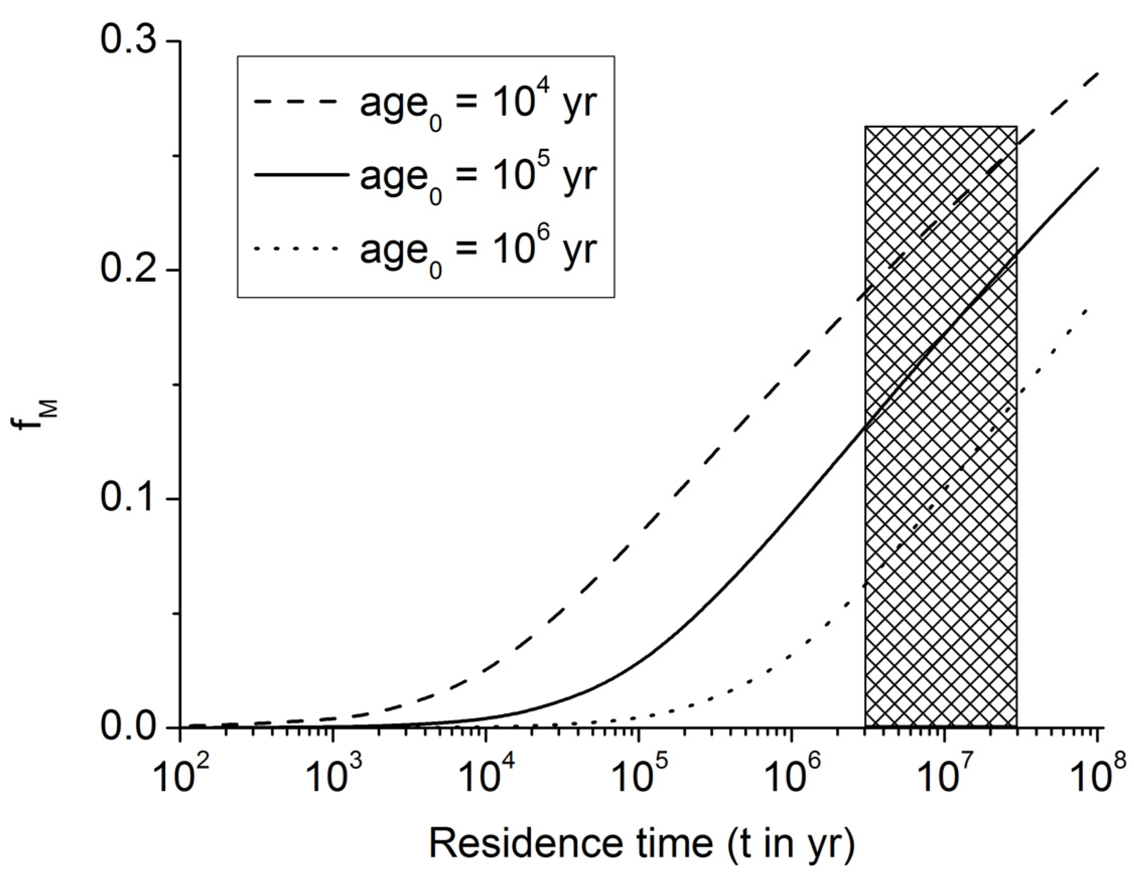
Figure 6. Fraction of POC converted into methane carbon within the methanogenic zone of continental margin sediments (f_M). The marked area indicates the range of POC residence times (t = 3–30 Myr) within the methanogenic zone at continental margins.

Figure 6. Fraction of POC converted into methane carbon within the methanogenic zone of continental margin sediments (f_M). The marked area indicates the range of POC residence times (t = 3–30 Myr) within the methanogenic zone at continental margins.

The residence time of sediments within the methanogenic zone is limited by the geothermal gradient since microbial methane formation cannot proceed at temperatures above ~100 °C. Assuming a geothermal gradient of 30–40 °C/km, the deep biosphere may extend to a sediment depth of about 3 km. At continental margins with typical burial velocities of 10–100 cm kyr⁻¹, the residence time within the methanogenic zone may thus fall into a range of t = 3–30 Myr. Figure 6 and Equation (12) show that about 10%–20% of the POC entering the methanogenic zone is microbially converted into methane under these assumptions (for age₀ = 10⁵ yr). Since 30–90% of POC buried below the bioturbated surface zone of continental margin sediments is reaching the methanogenic zone (Figure 5), about 3%–18% of the buried POC is converted into methane by the deep biosphere residing in underlying sulfate-depleted sediment layers.

Considering the arguments and equations presented above it is now possible to estimate the rate of microbial methane formation in continental margin sediments at global scale (Table 1).

Table 1. Quaternary POC and methane balance for global continental margins.

	Range	Best Estimate
POC burial at continental margins (1014 g C yr−1)	1.21–1.39	1.3
Fraction of buried POC reaching the methanogenic zone (%)	30–90	50
Fraction of buried POC microbially converted into methane (%)	3–18	8
Microbial methane production rate (1012 g C yr−1)	4–25	10

Table 1. Quaternary POC and methane balance for global continental margins.

	Range	Best Estimate
POC burial at continental margins (1014 g C yr−1)	1.21–1.39	1.3
Fraction of buried POC reaching the methanogenic zone (%)	30–90	50
Fraction of buried POC microbially converted into methane (%)	3–18	8
Microbial methane production rate (1012 g C yr−1)	4–25	10

This new estimate of microbial methane production in margin sediments (4–25 Tg C yr⁻¹, Table 1) is significantly lower than previous estimates of the global microbial methane production ranging from 60 Tg C yr⁻¹ [38] to 240 Tg C yr⁻¹ [39]. These previous estimates approach or even exceed the global rate of POC burial below the bioturbated zone. Our best estimate of ~10 Tg C yr⁻¹ would lead to an accumulation of up to 100,000 Gt CH₄-C over an accumulation period of 10 Myr if none of the methane would be lost by upward diffusion, AOM, fluid flow and gas ascent. However, field data clearly show that a large fraction of methane is lost by upward diffusion and fluid flow into the overlying sulfate-bearing zone where methane is consumed by microbial consortia using sulfate as terminal electron acceptor [24]. The biogenic methane inventory is thus certainly much smaller than the time-integrated rate of biogenic methane formation derived above. Nevertheless, the number of 100,000 Gt C is a useful upper limit for biogenic methane accumulation. Interestingly, the global methane hydrate inventory estimated by Klauda and Sandler [4] approaches this upper limit value.

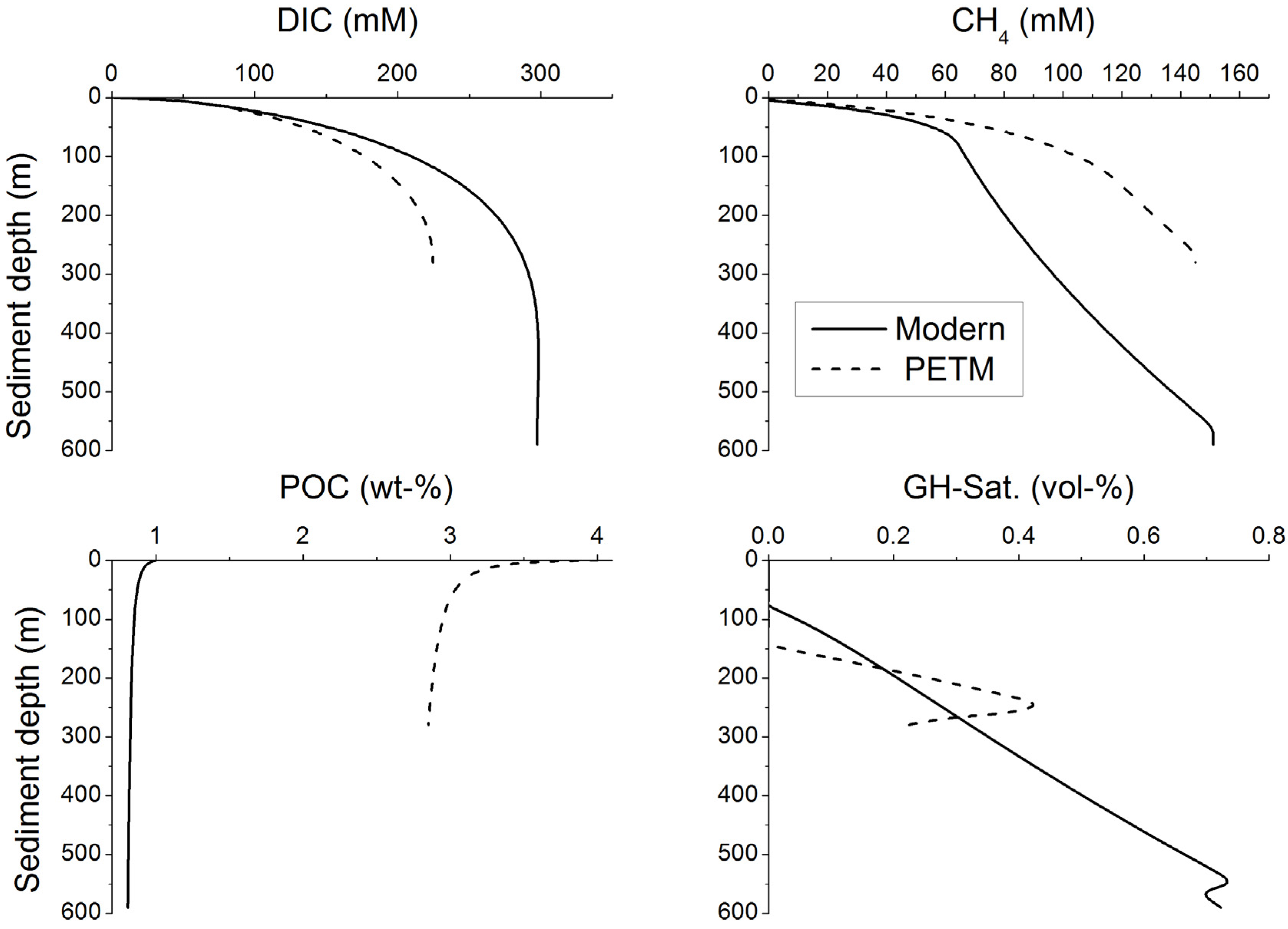
The kinetic models of Middelburg and Wallmann can also be used to estimate the total POC degradation rate within the deep marine biosphere. The Middelburg model [Equation (8)] yields a rate of 1.2 × 10¹⁴ g yr⁻¹ applying a mean POC input flux of 1.4 × 10¹⁴ g yr⁻¹, an initial age of 10⁴ yr and a POC residence time in the deep biosphere of 10 Myr. It predicts that almost 90% of the buried POC would be consumed within the deep biosphere. Applying the same parameter values, an inhibition constant of 40 mM and mean methane and CO₂ concentrations of 50 mM, the Wallmann model [Equation (11)] predicts a POC consumption rate of 0.7 × 10¹⁴ g yr⁻¹ corresponding to ~50% of the burial flux. The remaining POC is further decomposed below the deep biosphere via chemical processes yielding thermogenic gas, oil, kerogen and other products of high-temperature (>100 °C) thermal maturation. It should, however, be noted that the numbers given above are very rough estimates since microbial organic matter degradation in the deep biosphere is a very complex and poorly understood process.

4. Thickness of the Gas Hydrate Stability Zone

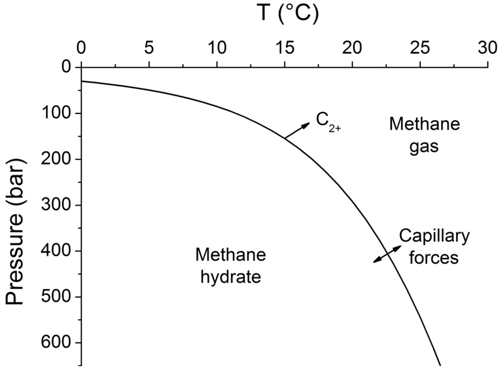
Methane hydrates are only stable at low temperatures and high pressures. The stability field of structure type-I methane hydrate is well defined [40]. Pitzer equations can be used to constrain the effects of seawater salinity and porewater composition on methane hydrate stability [34]. The stability field for sulfate-free seawater with a salinity of 35 PSU is shown in Figure 7. The sharp phase boundary depicted in Figure 7 is however not strictly valid for sediments and other porous media. Capillary forces acting on gas hydrates and free gas residing in sediment pores of different sizes create a broad transition zone where free gas and gas hydrate coexist [41]. The thickness of this zone has been estimated as 20–28 m for Hydrate Ridge and Blake Ridge [41]. The seismic bottom simulating reflector (BSR) indicating the top of the free gas occurrence zone is therefore often located at shallower depths than predicted by the bulk phase boundary. Moreover, the composition of the hydrate-forming natural gas has a strong effect on the positioning of the phase boundary. Biogenic gas formed by the microbial degradation of organic matter is composed of methane and CO₂ and contains only trace amounts of higher hydrocarbons (C₂₊). CO₂ hydrates are usually not formed in marine sediments since their solubility clearly exceeds the CO₂ concentration in ambient pore fluids. Methane hydrates are less soluble and therefore the major product of biogenic gas formation in marine sediments. The hydrate-bound gas thus typically contains more than 99.9% methane with only trace amounts of CO₂ and C₂₊ [42]. The low abundance of higher hydrocarbons in biogenic gas supports the formation of structure type I methane hydrate. However, thermogenic gas ascending from larger sediment depths contains significant amounts of C₂₊ favoring the formation of structure type II and/or the inclusion of C₂₊-components in structure type I methane hydrate. These hydrates are stable over a significantly broader P-T range and thus induce a down-core displacement of the phase boundary [40].

Figure 7. Phase diagram for methane hydrate (structure type I) for sulfate-free seawater with a salinity of 35 [34]. Arrows indicate the formation of a transition zone by capillary forces and the broadening of the gas hydrate stability zone by higher hydrocarbon compounds (C₂₊).

Figure 7. Phase diagram for methane hydrate (structure type I) for sulfate-free seawater with a salinity of 35 [34]. Arrows indicate the formation of a transition zone by capillary forces and the broadening of the gas hydrate stability zone by higher hydrocarbon compounds (C₂₊).

The thickness of the gas hydrate stability zone (GHSZ) in marine sediments is usually estimated considering the temperature (T) and pressure (P) conditions at the seabed and the increase in T and P with sediment depth. High-resolution data sets are available to define temperatures and pressures at the seafloor on global scale [6] while the conductive heat flux has been measured at more than 9000 sites [43]. Most of these heat flow data have been generated by measuring the temperature gradient within the upper few meters of the sediment column. The conductive heat flux (q_H) is then calculated from the temperature gradient considering the ambient thermal conductivity of bulk sediments (λ_B):

$$q_{\text{H}}={\lambda }_{\text{B}}\cdot \frac{\partial T}{\partial z}$$

(13)

Heat flow data rather than temperature gradients (dT/dz) have been compiled at global scale [43]. Geothermal gradients defining the thickness of the gas hydrate stability zone, thus, need to be derived from the heat flux data applying appropriate estimates for ambient thermal conductivity. Thermal conductivities of bulk sediments quantify the efficiency of heat transport which involves transport (1) from grain to grain; (2) from grain to liquid to grain; and (3) through pore-filling liquid [44]. Rather than calculate the contribution of each heat transport path explicitly, thermal conductivity is often estimated using a two-phase mixing model to combine the thermal conductivities of the sediment grains with the pore fluid. The thermal conductivities of methane hydrate and water differ by <10% at the temperatures found in hydrate-bearing sediments [44]. For this reason, first-order thermal conductivity estimates can neglect the presence of methane hydrate and assume that the sediment pore space contains only water [45]. The following two-phase mixing model provides a reasonable approximation for thermal conductivity in the uppermost 500–1000 m of the sediment column [45]:

$${\lambda }_{\text{B}}={\lambda }_{\text{W}}{}^{\Phi }\cdot {\lambda }_{\text{S}}{}^{(1-\Phi )}$$

(14)

where λ_B, λ_W, and λ_S are thermal conductivities of bulk sediment, seawater and solids, respectively. The thermal conductivity of seawater increases with pressure and temperature [46]. It varies from 0.56 to 0.60 W m⁻¹ K⁻¹ over the P-T range encountered within the GHSZ [46]. A mean value of λ_W = 0.58 W m⁻¹ K⁻¹ is thus representative for the marine hydrate stability zone. Quartz has a conductivity of 7.7–8.4 W m⁻¹ K⁻¹ [44] while calcite has an average conductivity of 3.6 W m⁻¹ K⁻¹ [47]. Thermal conductivities of clay minerals vary from 5.2 W m⁻¹ K⁻¹ for chlorite to 1.8–2.7 W m⁻¹ K⁻¹ for smectite, illite and kaolinite [47]. Data measured in ODP cores retrieved at various continental margin sites indicate a mean value of λ_S = 2.5 W m⁻¹ K⁻¹ for the dry solids in fine-grained margin sediments [45]. The average porosity within the upper few meter of the sediment column is typically close to 0.75 [45]. Applying Equation (14), the thermal conductivity of clay-rich surface sediments results as λ_B = 0.836 W m⁻¹ K⁻¹ for λ_W = 0.58 W m⁻¹ K⁻¹ and λ_S = 2.5 W m⁻¹ K⁻¹. The geothermal gradient in surface sediments is thus derived by dividing the ambient heat flux data by λ_B = 0.836 W m⁻¹ K⁻¹ [Equation (13)].

Thermal conductivity changes, however, with sediment depth due to the compaction of sediments inducing a down-core decrease in porosity. Porosity change is often described by the following equation [19]:

$$\Phi ={\Phi }_{\text{f}}+\left({\Phi }_0-{\Phi }_{\text{f}}\right)\cdot e^{-p\cdot z}$$

(15)

where Φ₀ is the porosity at the sediment surface, Φ_f the porosity at the base of the sediment column and p is an attenuation coefficient. The mean porosity profile observed in ODP cores can be approximated applying Φ₀ = 0.74, Φ₀ = 0.3 and p = 1/600 m⁻¹ [48].

The steady-state temperature profile in marine sediments is usually controlled by heat conduction. Neglecting heat production and convection, it can be described by the following differential equation [49]:

$$\frac{\partial }{\partial z}\cdot \left({\lambda }_{\text{B}}\cdot \frac{\partial T}{\partial z}\right)=0$$

(16)

This equation can be solved applying the following boundary conditions at the top of the sediment column at z = 0:

$$\frac{\partial T}{\partial z}=T_{\text{Grad}}=\frac{q_{\text{H}}}{{\lambda }_{\text{B}}}T=T_{\text{BW}}$$

(17)

where T_Grad is the temperature gradient recorded in surface sediments, q_H is the heat flow calculated from the gradient and the thermal conductivity of surface sediments while T_BW is the temperature of ambient bottom water. The solution of this equation for constant λ_B results as:

$$T=T_{\text{BW}}+T_{\text{Grad}}$$

(18)

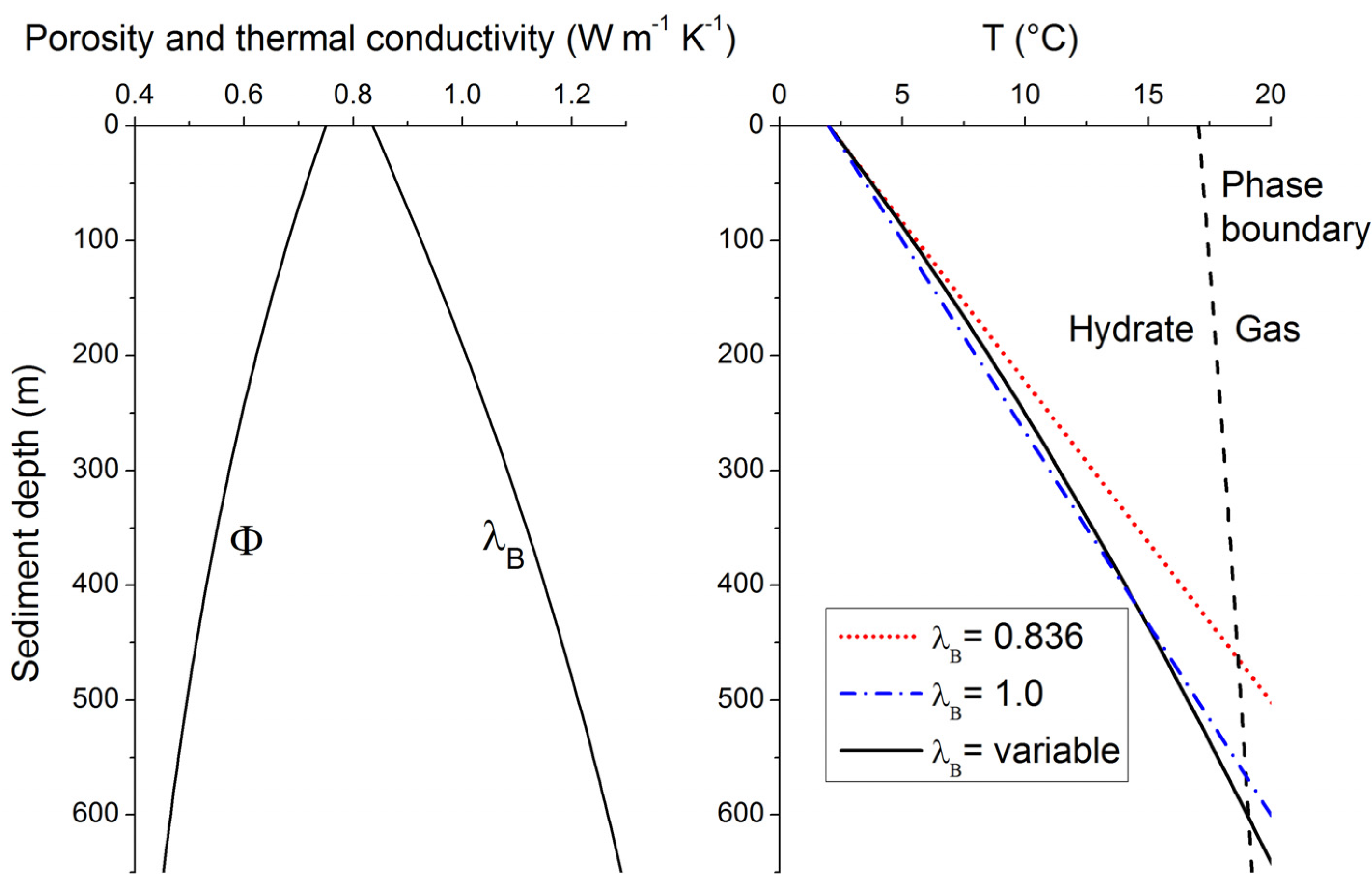
The equation can also be solved for variable λ_B considering the down-core changes in porosity and λ_B defined in Equations (14,15). The resulting temperature profile is depicted in Figure 8 for typical continental margin sediments (solid black line in the right panel). It shows a clearly non-linear shape since the down-core decrease in porosity induces a significant λ_B increase with depth (left panel in Figure 8). The linear profile calculated from the λ_B value in surface sediments [λ_B = 0.836 W m⁻¹ K⁻¹, red dotted line in the left panel, Equation (16)] overestimates sediment temperatures at depth and thus underestimates the thickness of the GHSZ by almost 150 m (Figure 8). It is thus important to consider the non-linear nature of sedimentary temperature profiles. The temperature profile and GHSZ thickness can, however, be approximated applying a constant λ_B of 1 W m⁻¹ K⁻¹ (blue dotted-broken line in right panel of Figure 8). This mean value is thus often applied to estimate the vertical extent of the GHSZ in marine sediments [45].

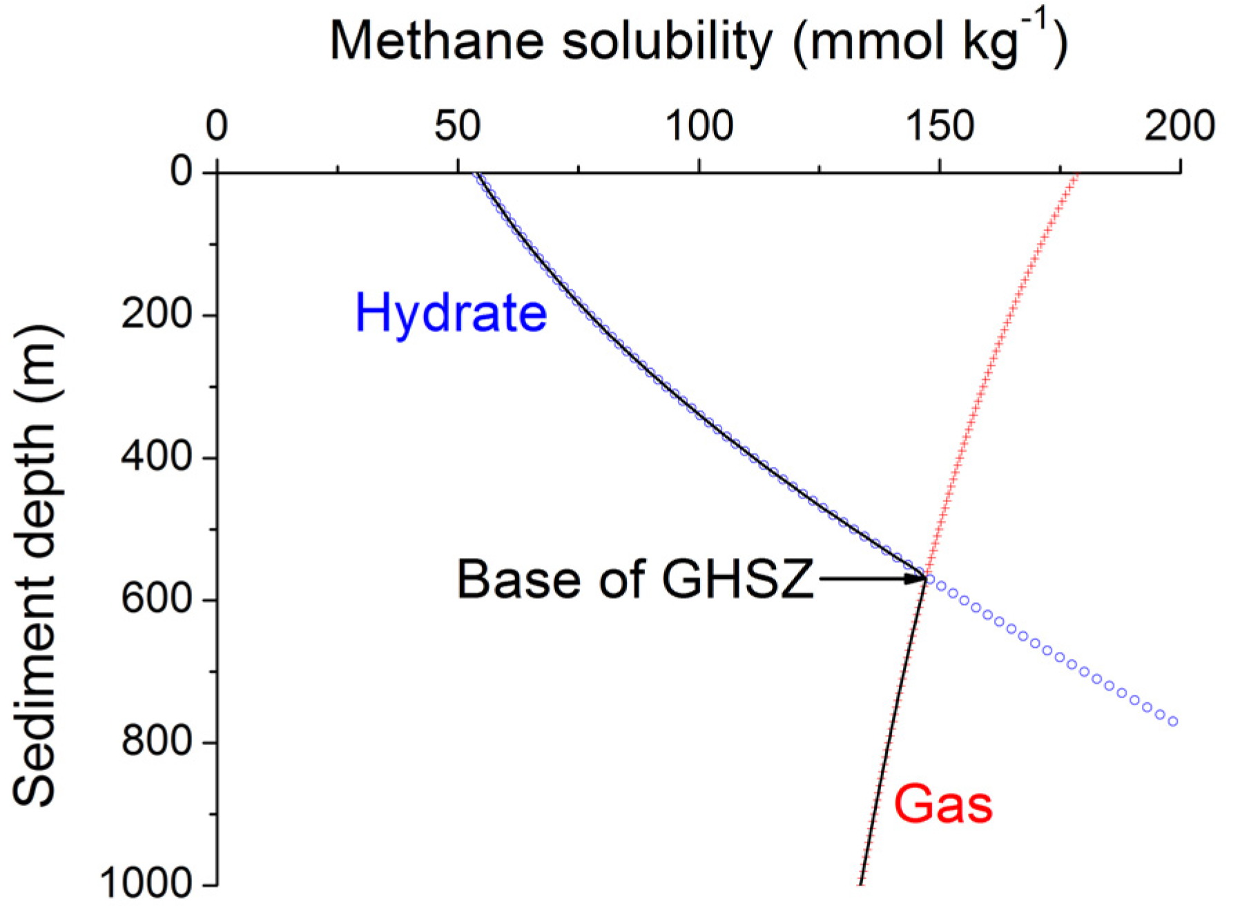
Global maps of the GHSZ thickness were produced by Burwicz et al. [6] and Pinero et al. [50] assuming constant temperature gradients and applying the same global data sets for water depth, bottom water temperature, heat flow and sediment thickness. The base of the GHSZ is defined by the intersection of the sedimentary temperature profile and the phase boundary for sulfate-free pore water (Figure 8). Pinero et al. 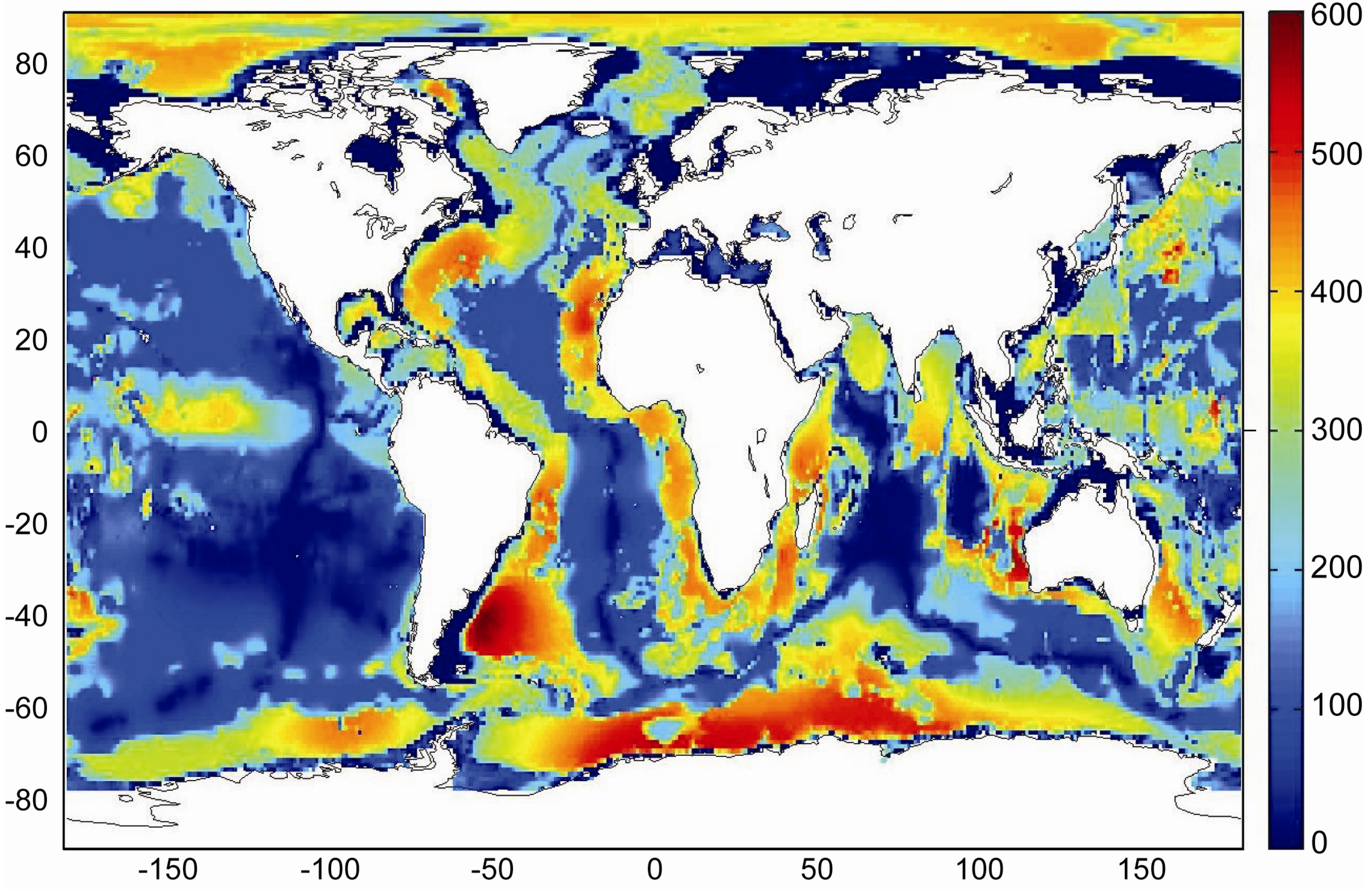[50] assumed a constant thermal conductivity of λ_B = 1.0 W m⁻¹ K⁻¹ over the entire ocean. The map produced under this assumption gives a good approximation for the GHSZ thickness in fine-grained continental margin sediments (Figure 9). The vertical extend of the GHSZ is, however, underestimated where sediments are dominated by sand, chlorite and calcite since sedimentary bulk conductivity is strongly enhanced by these components [47]. Moreover, the map is based on a thermodynamic model valid for pure methane hydrate of structure type I [34]. It may thus underestimate the vertical extent of the GHSZ where methane hydrate is stabilized by C₂₊ components entrained into the GHSZ by the ascent of thermogenic gas (Figure 7). Burwicz et al. [6] applied a constant λ_B value of 1.5 W m⁻¹ K⁻¹ which over-predicts the GHSZ thickness in margin sediments composed of smectite, illite and kaolinite but may give a better approximation for pelagic sediments. Both maps show an extended and deep-reaching GHSZ at high latitudes and around passive continental margins whereas a thin GHSZ is derived for the open ocean where the thickness of the GHSZ is limited by the thin sedimentary cover.

Figure 8. Down-core change in porosity [Φ, Equation (15)], thermal conductivity of bulk sediment [λ_B, Equation (14)] and temperature [T, Equation (16)] in typical continental margin sediments (Φ₀ = 0.74, Φ_f = 0.3 and p = 1/600 m⁻¹, q_H = 0.03 W m⁻², λ_W = 0.58 W m⁻¹ K⁻¹, λ_S = 2.5 W m⁻¹ K⁻¹). The phase boundary for methane hydrate (structure type I) shown in the right panel (black broken line) is calculated for sediments deposited at 2000 m water depth, hydrostatic pressure conditions and sulfate-free sediment porewater with a salinity of 35 [34].

Figure 8. Down-core change in porosity [Φ, Equation (15)], thermal conductivity of bulk sediment [λ_B, Equation (14)] and temperature [T, Equation (16)] in typical continental margin sediments (Φ₀ = 0.74, Φ_f = 0.3 and p = 1/600 m⁻¹, q_H = 0.03 W m⁻², λ_W = 0.58 W m⁻¹ K⁻¹, λ_S = 2.5 W m⁻¹ K⁻¹). The phase boundary for methane hydrate (structure type I) shown in the right panel (black broken line) is calculated for sediments deposited at 2000 m water depth, hydrostatic pressure conditions and sulfate-free sediment porewater with a salinity of 35 [34].

Figure 9. Thickness of the gas hydrate stability zone calculated from global heat flux data [43] considering bathymetry, bottom water temperature, sediment thickness data and a bulk thermal conductivity of 1.0 W m⁻¹ K⁻¹ [50].

Figure 9. Thickness of the gas hydrate stability zone calculated from global heat flux data [43] considering bathymetry, bottom water temperature, sediment thickness data and a bulk thermal conductivity of 1.0 W m⁻¹ K⁻¹ [50].

The global volume of the GHSZ is estimated to be 67 × 10¹⁵ m³ integrating the data shown in Figure 9. This value should be considered as a minimum estimate since the thickness of the GHSZ may be underestimated in those areas where solid phases with high thermal conductivity and C₂₊-bearing gas hydrates are deposited. The pore space available for gas hydrate accumulation amounts to 44 × 10¹⁵ m³ considering the decay of porosity over the sediment column [Figure 8, Equation (15)]. Up to 4 × 10²¹ g CH₄-C could reside in the GHSZ if the entire pore space (44 × 10¹⁵ m³) would be filled by methane hydrate. This maximum estimate clearly exceeds the total methane pool generated via microbial POC degradation over a period of 10 Myr (1.0 × 10²⁰ g CH₄-C, see section 3). Thus, only 2.5% of the global GHSZ pore space could be occupied by gas hydrates if the entire biogenic methane pool would be fixed as gas hydrate.

5. Solubility of Methane in Sedimentary Pore Fluids

Methane produced by the microbial degradation of organic matter is dissolved in ambient pore fluids. The solubility of methane in water is however limited by the low polarity and hydrophobic nature of methane molecules. Excess methane formed by pervasive methane production thus precipitates as gas hydrate or forms a free gas phase pending on the local P-T conditions. Methane hydrate precipitates when the methane concentration in the pore fluids exceeds the solubility of methane hydrate. The equilibrium concentration with respect to methane hydrate is restored by hydrate precipitation extracting excess methane from solution. The solubility of methane hydrate has been measured experimentally and calculated using various thermodynamic approaches [44]. It increases with temperature and decreases with pressure and salinity whereas the solubility of methane gas in water is enhanced under high pressure and reduced by an increase in temperature and salinity. The down-core rise in sediment temperature thus promotes an increase in dissolved methane concentrations within the GHSZ and a decrease in dissolved methane in the underlying free gas zone (Figure 10).

Figure 10. Solubility of methane in marine sediments deposited at 2000 m water depth. Solubility is calculated for methane hydrate (blue circles) and methane gas (red crosses) in sulfate-free seawater with S = 35 assuming hydrostatic conditions, a bottom water temperature of 2 °C and a linear geothermal gradient of 0.03 °C m⁻¹ [34,51]. The black line indicates the dissolved methane concentration attained in methane-saturated pore fluids (in mmol per kg solution). The base of the gas hydrate stability zone (GHSZ) is located at the intersection of the gas hydrate and free gas solubility curves.

Figure 10. Solubility of methane in marine sediments deposited at 2000 m water depth. Solubility is calculated for methane hydrate (blue circles) and methane gas (red crosses) in sulfate-free seawater with S = 35 assuming hydrostatic conditions, a bottom water temperature of 2 °C and a linear geothermal gradient of 0.03 °C m⁻¹ [34,51]. The black line indicates the dissolved methane concentration attained in methane-saturated pore fluids (in mmol per kg solution). The base of the gas hydrate stability zone (GHSZ) is located at the intersection of the gas hydrate and free gas solubility curves.

Capillary forces affect the stability and solubility of gas hydrate and gas in fine-grained marine sediments. A transition zone is formed where the solubility ranges of gas bubbles and hydrate crystals residing in sediment pores of different sizes overlap [41]. The discontinuity at the base of the GHSZ (Figure 10) is thus replaced by a smooth and continuous transition in methane solubility [41,44].

6. Sediment Compaction, Fluid Flow and Gas Ascent

Gas hydrates are formed from methane being produced within the GHSZ (section 3) and by methane ascending into the GHSZ from below. Upward flow of methane is induced by numerous processes including sediment compaction, tectonic over-pressuring and the buoyancy of methane gas and methane charged fluids. Sediment compaction is driven by the overburden load of younger sediments being continuously deposited at the seabed [48]. In most marine settings, it induces an exponential decrease in porosity (Φ) and water content with sediment depth (Figure 8). Therefore, exponential equations such as Equation (15) are used to describe the compaction-driven down-core decrease in porosity. Applying Equations (1,15), the burial velocity of pore water (v_B) and solids (w_B) are calculated as [19]:

$$\begin{array}{l}{v}_{\text{B}}=\frac{{\Phi }_{\text{f}}\cdot w_{\text{f}}}{\Phi }{w}_{\text{B}}=\frac{\left(1-{\Phi }_{\text{f}}\right)\cdot w_{\text{f}}}{\left(1-\Phi \right)}\end{array}$$

(19)

The equations above are valid for steady state conditions, i.e., for homogenous deposits formed by continuous sedimentation. The porosity of marine sediments deposited on oceanic crust is usually not completely eliminated by compaction. The residual porosity at the base of the sediment column (i.e., the crust-sediment interface) is given by Φ_f while w_f is the burial velocity of water and solids which is attained after the porosity has been reduced to Φ_f via steady-state compaction. 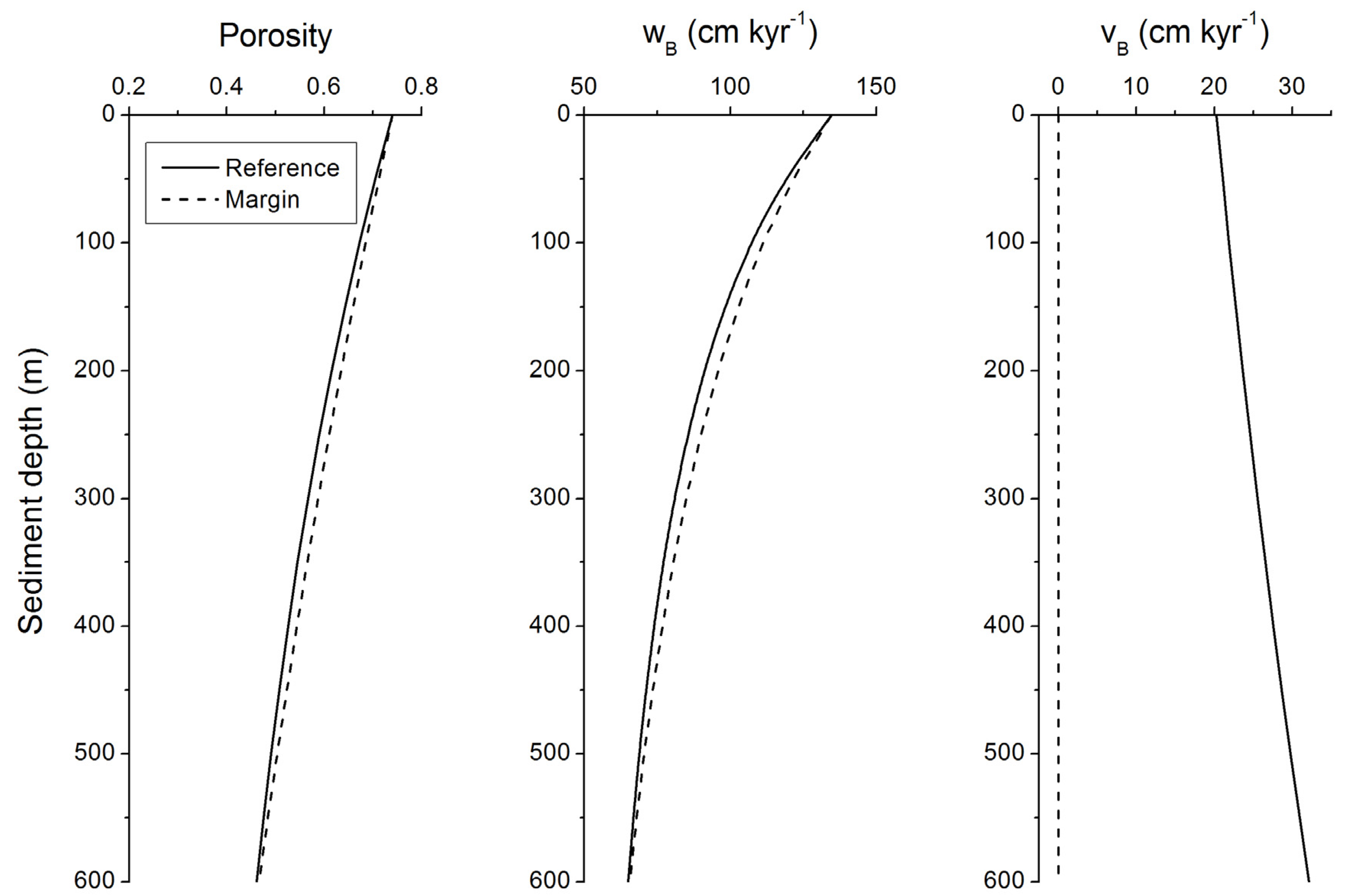Compaction promotes the burial of solids while pore water burial is diminished since water is expelled and transported upwards due to the down-core reduction in pore space (Figure 11). However, steady-state compaction does not induce a flow of water into the overlying water column: The pore fluids do not escape into the bottom water since the pore water burial velocity induced by the continuous deposition of young sediments at the seabed exceeds the velocity of the compaction-driven upward fluid flow.

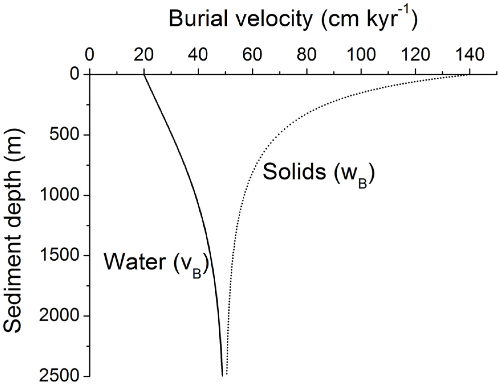
Figure 11. Burial velocity of pore fluids (v_B) and solids (w_B) in marine sediments subject to steady-state compaction. Velocities are calculated applying Equation (19) with Φ₀ = 0.74, Φ_f = 0.3, p = 1/600 m⁻¹, and w_f = 50 cm kyr⁻¹.

Figure 11. Burial velocity of pore fluids (v_B) and solids (w_B) in marine sediments subject to steady-state compaction. Velocities are calculated applying Equation (19) with Φ₀ = 0.74, Φ_f = 0.3, p = 1/600 m⁻¹, and w_f = 50 cm kyr⁻¹.

Seepage of pore fluids is frequently observed at continental margins where sediments are compressed by tectonic forces [52] since marine sediments subducted below continental crust and accreted at active continental margins are over-pressured and dewatered to such an extent that pore fluids escape into the bottom water [53,54,55,56]. Salt diapirism, sediment erosion and slope failure induce additional fluid seepage at passive and active continental margins. Upward fluid flow is ultimately driven by excess pressures as described by the Darcy equation [57]:

$$u=-\frac{k}{{\mu }_{\text{W}}}\cdot \left(\frac{\partial P}{\partial z}-{\rho }_{\text{W}}\cdot g\right)$$

(15)

where the Darcy flow u (m³ m⁻² yr⁻¹) is the volume of water (m³) being transported through a cross-sectional sediment area (m²) over a period of time (yr). Upward fluid flow occurs when the sedimentary pressure gradient ($\partial P$ in Pa m⁻¹) exceeds the hydrostatic pressure gradient defined as product of water density (ρ_W in kg m⁻³) and gravitational acceleration (g = 9.81 Pa m² kg⁻¹). The velocity of fluid flow is modulated by the intrinsic permeability of bulk sediments (k in m²) and the viscosity of water (µ_w ≈ 10⁻³ Pa s). The intrinsic permeability of marine sediment varies over several orders of magnitude. It increases with porosity and grain size: Terrigenous marine sediments containing fine-grained clay have typical permeability values of 10⁻¹⁸–10⁻¹⁴ m² while clean sands have values of 10⁻¹²–10⁻¹⁰ m² [57].

The sedimentary pressure gradient is enhanced in compressive tectonic settings and may approach the lithostatic pressure gradient defined as the product of g and the bulk density of sediments. The bulk density of sediments ρ_B is calculated as:

$${\rho }_{\text{B}}={\rho }_{\text{W}}\cdot \Phi +{\rho }_{\text{S}}\cdot \left(1-\Phi \right)$$

(21)

The Darcy flow at lithostatic pressure u_L is thus calculated as:

$$u_{\text{L}}=-\frac{k}{{\mu }_{\text{W}}}\cdot \left({\rho }_{\text{B}}\cdot g-{\rho }_{\text{W}}\cdot g\right)=-\frac{k\cdot g}{{\mu }_{\text{W}}}\cdot \left({\rho }_{\text{W}}\cdot \left(\Phi -1\right)+{\rho }_{\text{S}}\cdot \left(1-\Phi \right)\right)$$

(22)

The inter-granular fluid flow velocity v is related to the Darcy flow velocity u as:

$$v=\frac{u}{\Phi }$$

(23)

Both velocities, u and v, attain a positive sign for a downward movement with respect to the sediment-water interface while a negative sign indicates the ascent of pore fluids towards the sediment surface. Fluids ascending through a constantly growing homogenous sediment deposit subject to steady-state compaction have an inter-granular fluid flow velocity of:

$$v_{\text{N}}=v+v_{\text{B}}=\frac{u+{\Phi }_{\text{f}}\cdot w_{\text{f}}}{\Phi }$$

(24)

Fluids are thus expelled across the sediment-water interface into the overlying water column when the velocity of fluids infiltrating the sediment column from below (v) exceeds the burial velocity of pore fluids (v_B). Upward fluid flow velocities (v) have been measured at various cold seep sites and mud volcanoes located at active and passive continental margins [53,54,58,59,60,61,62,63]. They typically range from 0.1 to 100 cm yr⁻¹. 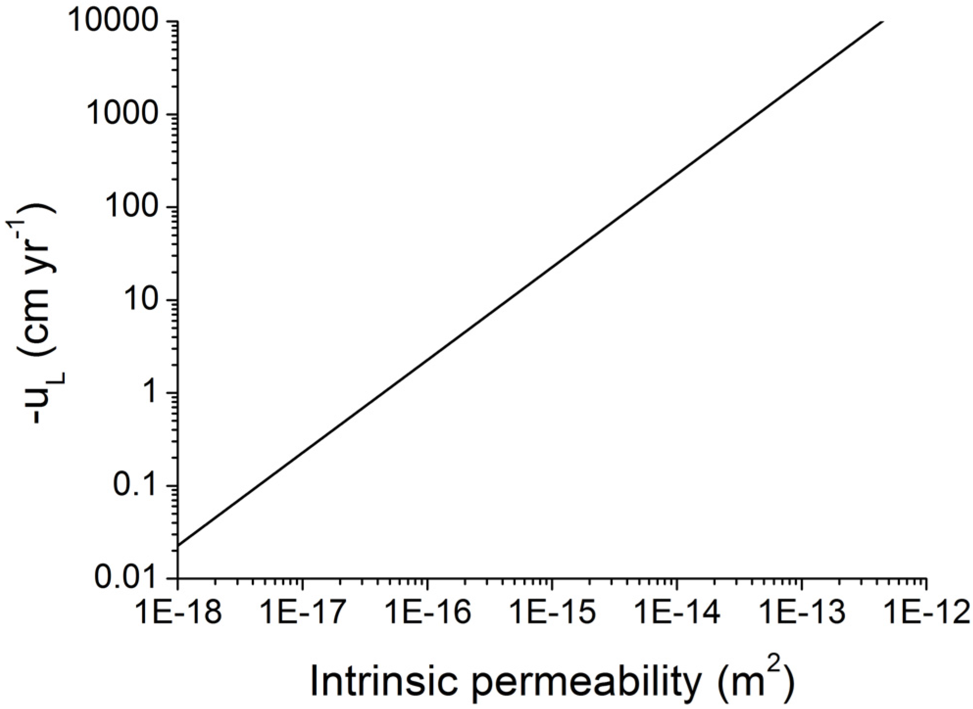These flow velocities are consistent with u_L values predicted for over-pressured clay-bearing sediments deposited at continental margins (Figure 12).

Figure 12. Velocity of Darcy fluid flow at lithostatic pressure (u_L) in marine sediments as function of intrinsic permeability. Darcy flow is calculated applying density values of ρ_W = 1036 kg m⁻³ and ρ_S = 2500 kg m⁻³ and a porosity of Φ = 0.5.

Figure 12. Velocity of Darcy fluid flow at lithostatic pressure (u_L) in marine sediments as function of intrinsic permeability. Darcy flow is calculated applying density values of ρ_W = 1036 kg m⁻³ and ρ_S = 2500 kg m⁻³ and a porosity of Φ = 0.5.

Gaseous methane occurs below the GHSZ and in the transition zone at the base of the GHSZ. The bottom simulating reflector (BSR) observed in many seismic surveys marks the boundary between hydrate-bearing sediments and the underlying gas-bearing sediment zone. The density of methane gas is lower than the density of pore fluids. Therefore buoyancy forces may induce an upward flow of gas into the GHSZ. For sediments containing both gas and water, Darcy’s law is formulated as [57]:

$$\begin{array}{l}{u}_{\text{W}}=-\frac{k\cdot k_{\text{RW}}}{{\mu }_{\text{W}}}\cdot \left(\frac{\partial P_{\text{W}}}{\partial z}-{\rho }_{\text{W}}\cdot g\right)u_{\text{G}}=-\frac{k\cdot k_{\text{RG}}}{{\mu }_{\text{G}}}\cdot \left(\frac{\partial P_{\text{G}}}{\partial z}-{\rho }_{\text{G}}\cdot g\right)\end{array}$$

(25)

where the subscripts W and G indicate water and gas, respectively. Relative permeability appears as additional non-dimensional parameter in the equations above (k_RW and k_RG). Various equations have been proposed to quantify the relative permeability of water and gas in marine sediments at different saturation values [44,57]. One of the more commonly used forms is given by [64]:

$$\begin{array}{l}{k}_{\text{RW}}=S_{\text{WN}}{}^{\raisebox{1ex}{$1$}\!\left/ \!\raisebox{-1ex}{$2$}\right.}\cdot {\left(1-{\left(1-S_{\text{WN}}{}^{\raisebox{1ex}{$1$}\!\left/ \!\raisebox{-1ex}{$m$}\right.}\right)}^m\right)}^2{k}_{\text{RG}}={\left(1-S_{\text{WN}}\right)}^{\raisebox{1ex}{$1$}\!\left/ \!\raisebox{-1ex}{$2$}\right.}\cdot {\left(1-S_{\text{WN}}{}^{\raisebox{1ex}{$1$}\!\left/ \!\raisebox{-1ex}{$m$}\right.}\right)}^{2m}\end{array}$$

(26)

where m is the pore-size-distribution index. The normalized water saturation S_WN is defined as:

$$S_{\text{WN}}=\text{min\hspace{0.17em}}\left[\frac{S_{\text{W}}-S_{\text{WC}}}{1-S_{\text{WC}}-S_{\text{GC}}},1\right]$$

(27)

where S_W is the water saturation, i.e., fraction of pore space occupied by water (S_W = 1 − S_G). The irreducible water saturation has a typical value of S_WC = 0.3 while the corresponding gas saturation falls into the range of S_GC = 0.01–0.1 [65]. The irreducible gas saturation is the most critical parameter for the prediction of upward gas migration in marine sediments since gas migration occurs only when the gas saturation S_G exceeds S_GC. A high S_GC value of 0.1 indicates that gas migration is inhibited if less than 10% of the pore space is occupied by gas [S_G < 0.1, S_WN = 1, k_RG = 0, q_G = 0, s. Equations (25–27)]. This would imply that gas migration across the BSR is effectively suppressed since the methane gas produced by microbial POC degradation below the GHSZ rarely builds up to saturations of S_G > 0.1. The BSR is produced by the strong seismic contrast between gas below the GHSZ and gas hydrate within the GHSZ. Seismic surveys show a wide-spread occurrence of the BSR indicating that a significant fraction of methane gas is not mobile but retained and buried in sediments underlying the GHSZ. However, seismic chimneys indicating the ascent of free gas are also frequently observed at continental margins and are often associated with high gas hydrate saturations in the overlying GHSZ. It thus seems that the free gas is usually immobile but locally mobilized and transported into the GHSZ. The controls on gas migration into the GHSZ are poorly understood and this lack of physical understanding causes a large degree of uncertainty in the prediction of gas hydrate accumulation in marine sediments.

The gas pressure P_G is related to the water pressure P_W as [57]:

$$P_{\text{G}}=P_{\text{W}}+P_{\text{C}}$$

(28)

where P_C is the capillary pressure. P_C may be calculated as [66]:

$$P_{\text{C}}=P_{\text{CC}}\cdot {\left(S_{\text{WN}}{}^{\left(\frac{-npc}{npc-\text{1}}\right)}-1\right)}^{\frac{1}{npc}}$$

(29)

where P_CC has a value of 13,300 Pa in low permeability sediments while npc takes a value of 1.7 [66].

Darcy gas flow at constant gas saturation ($\partial \hspace{0.17em}{P}_C/\partial z=0$) and hydrostatic pressure ($\partial P_G/\partial z=\partial P_W/\partial z=g\cdot {\rho }_W$) can be calculated as function of gas saturation (S_G) and intrinsic permeability to quantify the buoyancy driven gas ascent into the GHSZ:

$$u_{\text{G}-\text{H}}=-\frac{k\cdot k_{\text{RG}}\cdot g}{{\mu }_{\text{G}}}\cdot \left({\rho }_{\text{G}}-{\rho }_{\text{W}}\right)$$

(30)

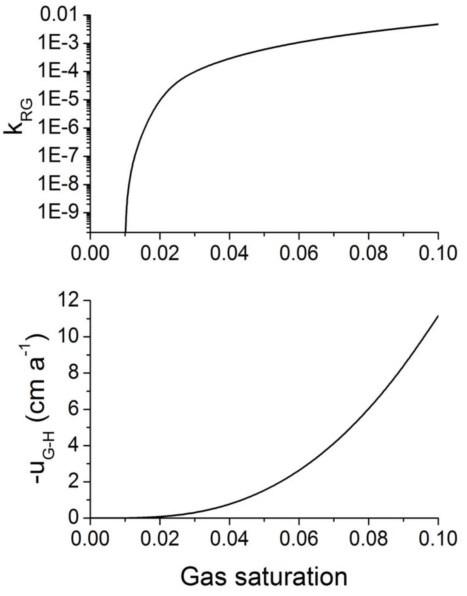
Figure 13 shows this buoyancy driven flux for typical continental margin sediments deposited at 2000 m water depth. Applying a geothermal gradient of 30 °C/km, the temperature at the base of the GHSZ is 19.1 °C while the hydrostatic pressure at the phase boundary amounts to 257 bar (Figure 8). The densities of methane gas and water are ρ_G = 198 kg m⁻³ [67] and ρ_W = 1036 kg m⁻³ [68] under these P-T conditions while the dynamic viscosity of methane gas amounts to µ_G = 11 × 10⁻⁶ Pa s [69]. The gas flow is completely inhibited at S_G < S_GC and increases rapidly with increasing S_G at S_G > S_GC. Buoyancy forces would thus induce a rapid ascent of gas into the GHSZ if the gas saturation exceeds the critical value. Under these conditions the methane hydrates buried and dissociated below the GHSZ would not be lost from the system but would be constantly recycled into the GHSZ via upward gas migration. The methane hydrate inventory would expand over time until the pore space available for gas migration is clocked by methane hydrate. Very high methane hydrate saturations could be attained by this recycling mechanism.

Figure 13. Relative permeability of gas [k_RG, upper panel, Equation (26)] and buoyancy-driven gas flow (u_G-H, lower panel, Equation 30) in fine-grained marine sediments as function of gas saturation (S_G = 1 − S_W). k_RG is calculated applying Equations 26 and 27 with S_WC = 0.3, S_GC = 0.01 and m = 0.75. The gas flux is calculated for hydrostatic pressure conditions applying Equation 30 with ρ_W = 1036 kg m⁻³, ρ_G = 198 kg m⁻³, k = 10⁻¹⁵ m², µ_G = 11 × 10⁻⁶ Pa s and the relative gas permeability depicted in the upper panel.

Figure 13. Relative permeability of gas [k_RG, upper panel, Equation (26)] and buoyancy-driven gas flow (u_G-H, lower panel, Equation 30) in fine-grained marine sediments as function of gas saturation (S_G = 1 − S_W). k_RG is calculated applying Equations 26 and 27 with S_WC = 0.3, S_GC = 0.01 and m = 0.75. The gas flux is calculated for hydrostatic pressure conditions applying Equation 30 with ρ_W = 1036 kg m⁻³, ρ_G = 198 kg m⁻³, k = 10⁻¹⁵ m², µ_G = 11 × 10⁻⁶ Pa s and the relative gas permeability depicted in the upper panel.

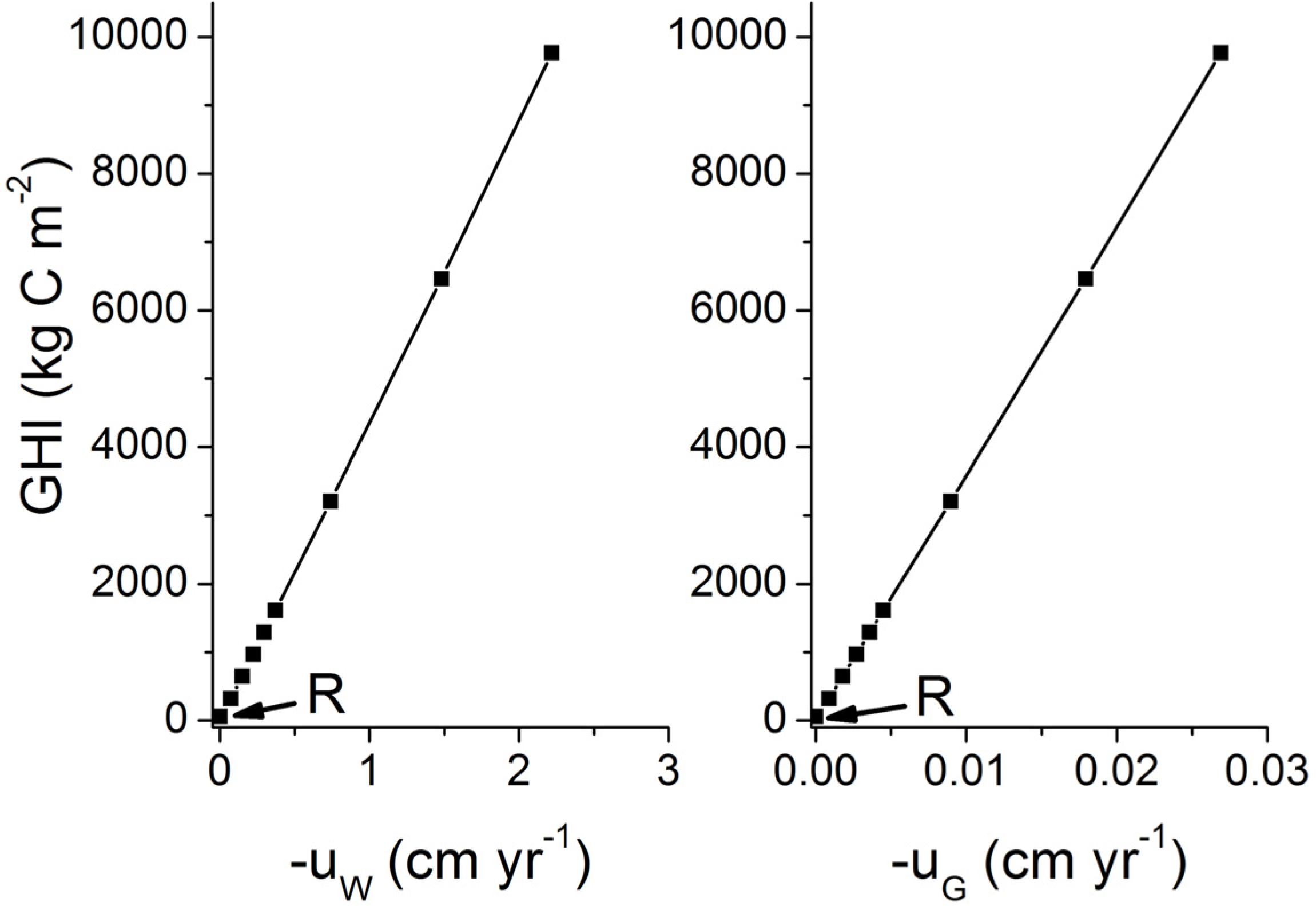
It is important to note that gas ascent is a much more efficient mechanism for the transport of methane into the GHSZ than fluid flow. For the conditions shown in Figure 13, an upward Darcy gas flow of 1 cm yr⁻¹ introduces a methane flux of 1980 g m⁻² yr⁻¹ (for ρ_G = 198 kg m⁻³) while a corresponding water flow of 1 cm yr⁻¹ induces a methane flux of only 24 g m⁻² yr⁻¹ at a dissolved methane concentration of 150 mM (Figure 10).

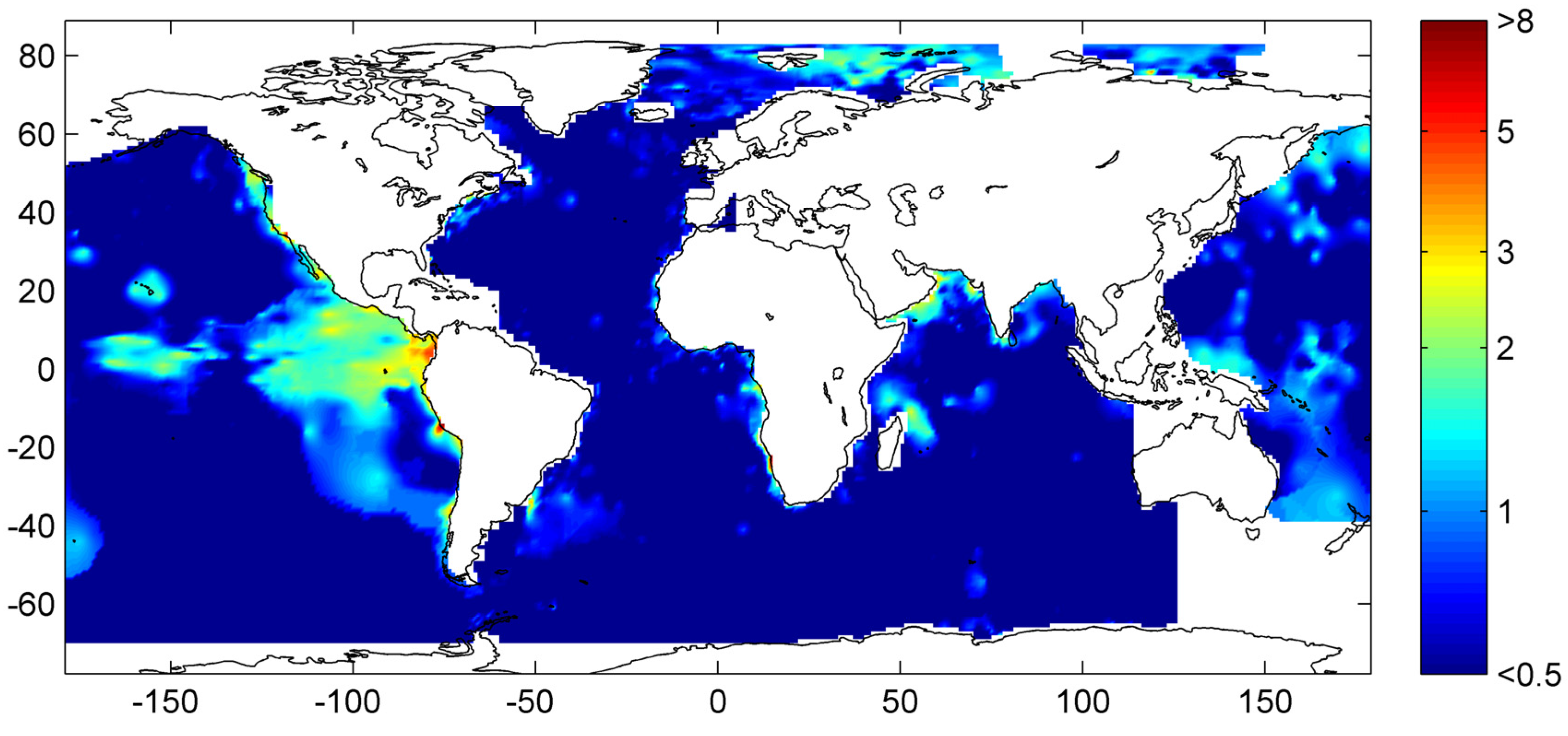
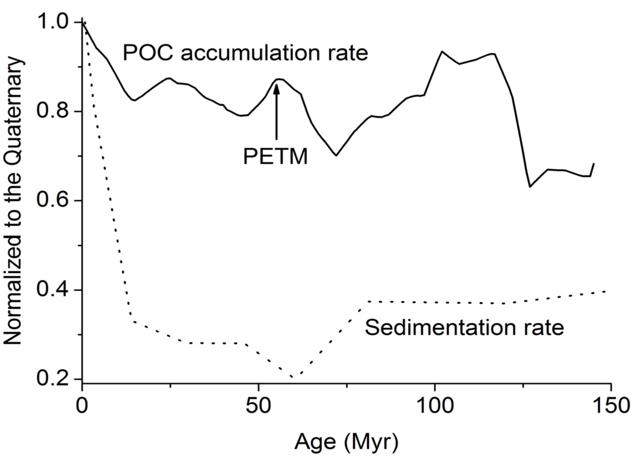
The POC accumulation rates that are fueling methane production at depth rarely exceed 10 g m⁻² yr⁻¹ (Figure 3). The entire methane pool potentially formed by the microbial and thermal decomposition of buried POC would thus be transported into the GHSZ at gas and water flow velocities as low as u_G ≈ 0.002 cm yr⁻¹ and u_W ≈ 0.2 cm yr⁻¹.

A better understand of the physical controls on gas and water ascent into the GHSZ is thus a high priory requirement for the prediction of gas hydrate accumulation at local and global scale.

7. Controls on Gas Hydrate Accumulation in Marine Sediments

In the following section we will present a series of model runs obtained with the transport-reaction model introduced by Wallmann et al. [23] to investigate the controls on gas hydrate accumulation. We will start this analysis by presenting the results of a reference simulation. The sensitivity tests presented in the following sections are based on this reference case.

7.1. Reference Case

The reference case presents a continental margin site at about 2000 m water depth with moderately high concentrations of POC and very high sedimentation rates. Porosity and temperature profiles applied in the standard case are shown in Figure 8, the corresponding methane solubility values are depicted in Figure 10 while the burial velocities of solids and pore fluids are shown in Figure 11. Parameter values used in this reference model run are listed in Table 2.

Table 2. Parameter values and upper boundary conditions applied in the reference case.

Parameter	Symbol	Value
Depth-independent parameter values
Density of pore water	ρW	1036 kg m−3
Density of dry sediments	ρS	2500 kg m−3
Density of methane hydrate	ρGH	912 kg m−3
Thermal conductivity	λB	1.0 W m−1 K−1
Heat flow	qH	0.03 W m−2
Pressure gradient (hydrostatic)	$\partial P/\partial z$	0.1016 bar m−1
Length of the model column	L	590 m
Thickness of the GHSZ	LGHSZ	567 m
Simulation time	t	≥5 Ma
Inhibition constant for POC degradation	KC	40 mM
Initial age of POC	age0	10,000 yr
Kinetic constant for AOM	kAOM	10 dm3 mol−1 yr−1
Kinetic constant for gas hydrate precipitation	kGHP	10−3 wt.% yr−1
Kinetic constant for gas hydrate dissolution	kGHD	10−3 yr−1
Porosity at the sediment surface	Ф0	0.74
Porosity after compaction	Фf	0.3
Attenuation coefficient for porosity decrease	p	1/600 m−1
Burial velocity at the sediment surface	w0	134.6 cm yr−1
Burial velocity after compaction	wf	0.05 cm yr−1
Mass accumulation rate	MAR	875 g m−2 yr−1
Conditions at the upper boundary
Pressure	P0	200 bar
Temperature	T0	2 °C
Dissolved sulfate concentration	CS(0)	28.9 mM
Dissolved methane concentration	CM(0)	10−6 mM
Dissolved inorganic carbon concentration	CC(0)	2.3 mM
POC concentration	CPOC(0)	1 wt.%
Gas hydrate concentration	CGH(0)	0 wt.%

Table 2. Parameter values and upper boundary conditions applied in the reference case.

Parameter	Symbol	Value
Depth-independent parameter values
Density of pore water	ρW	1036 kg m−3
Density of dry sediments	ρS	2500 kg m−3
Density of methane hydrate	ρGH	912 kg m−3
Thermal conductivity	λB	1.0 W m−1 K−1
Heat flow	qH	0.03 W m−2
Pressure gradient (hydrostatic)	$\partial P/\partial z$	0.1016 bar m−1
Length of the model column	L	590 m
Thickness of the GHSZ	LGHSZ	567 m
Simulation time	t	≥5 Ma
Inhibition constant for POC degradation	KC	40 mM
Initial age of POC	age0	10,000 yr
Kinetic constant for AOM	kAOM	10 dm3 mol−1 yr−1
Kinetic constant for gas hydrate precipitation	kGHP	10−3 wt.% yr−1
Kinetic constant for gas hydrate dissolution	kGHD	10−3 yr−1
Porosity at the sediment surface	Ф0	0.74
Porosity after compaction	Фf	0.3
Attenuation coefficient for porosity decrease	p	1/600 m−1
Burial velocity at the sediment surface	w0	134.6 cm yr−1
Burial velocity after compaction	wf	0.05 cm yr−1
Mass accumulation rate	MAR	875 g m−2 yr−1
Conditions at the upper boundary
Pressure	P0	200 bar
Temperature	T0	2 °C
Dissolved sulfate concentration	CS(0)	28.9 mM
Dissolved methane concentration	CM(0)	10−6 mM
Dissolved inorganic carbon concentration	CC(0)	2.3 mM
POC concentration	CPOC(0)	1 wt.%
Gas hydrate concentration	CGH(0)	0 wt.%

The model simulates the reactive transport of three dissolved species (DIC, sulfate, methane) and two solid species (POC and methane hydrate). Molecular diffusion, burial and compaction are considered as transport processes. The simulated reactions include POC degradation via sulfate reduction, AOM, methanogenesis, gas hydrate formation and gas hydrate dissolution. Fixed concentration values are applied at the upper boundary (Table 2) while zero gradients are used as lower boundary conditions for all dissolved species. The model domain excludes the upper bioturbated zone of the sediment column and includes the transition zone at the base of GHSZ where the saturation concentration of dissolved methane is assumed to be constant over a depth interval of 23 m (see section 4) [41]. All model results shown in the following figures and tables are valid for steady state conditions which were reached after a simulation time of ~3 Ma. The reference model does not consider gas and fluid ascent into the GHSZ from below.

The dissolved inorganic carbon concentrations calculated in the reference run show a continuous increase with sediment depth reflecting the microbial degradation of POC (Figure 14). Dissolved methane production starts at ~8 m sediment depth after sulfate is almost completely consumed by organic matter degradation and AOM (Figure 15). Dissolved methane increases down-core and reaches the saturation value with respect to methane hydrate at a sediment depth of ~86 m. At this point gas hydrate starts to form in the sediment column (Figure 14). Methane hydrate formation continues since the microbial production of methane within the GHSZ over-compensates the down-core increase in methane hydrate solubility. Close to the base of the GHSZ at ~545 m sediment depth, methane hydrate dissolves since the saturation level is no longer maintained by the sluggish methane production from aging POC. The saturation level is restored by methane hydrate dissolution in the deeper portion of the GHSZ (545–567 m) and by a combination of dissolution and dissociation in the underlying transition zone (567–590 m). Methane hydrate buried below the model domain to sediment depths >590 m dissociates to form dissolved and gaseous methane.

Figure 14. Concentrations of dissolved inorganic carbon (DIC), dissolved methane (CH₄), particulate organic carbon (POC) and methane hydrate saturation (GH-Sat.) in the reference model run. The dotted line in the upper right panel indicated the concentration of methane in equilibrium with methane hydrate.

Figure 14. Concentrations of dissolved inorganic carbon (DIC), dissolved methane (CH₄), particulate organic carbon (POC) and methane hydrate saturation (GH-Sat.) in the reference model run. The dotted line in the upper right panel indicated the concentration of methane in equilibrium with methane hydrate.

Figure 15. Concentrations of dissolved sulfate (solid line) and dissolved methane (dotted line) in surface sediments calculated in the reference model run. The shaded bar indicates the sediment layer where methane is oxidized by microbial consortia using sulfate as terminal electron acceptor (AOM zone). The AOM zone is equivalent to the sulfate-methane transition zone (SMTZ).

Figure 15. Concentrations of dissolved sulfate (solid line) and dissolved methane (dotted line) in surface sediments calculated in the reference model run. The shaded bar indicates the sediment layer where methane is oxidized by microbial consortia using sulfate as terminal electron acceptor (AOM zone). The AOM zone is equivalent to the sulfate-methane transition zone (SMTZ).

The modeling shows that only ~22% of the POC being deposited below the bioturbated zone (729 mmol m⁻² yr⁻¹, Table 3) is degraded within the GHSZ. The remaining portion is buried to larger sediment depths. Sulfate reduction contributes ~26% to the total POC degradation while most of the POC degradation (~74%) occurs within the methanogenic zone of the GHSZ. Sulfate diffusing into the sediment from above (52.8 mmol m⁻² yr⁻¹) is consumed via AOM (~60%) and POC degradation (~40%). The slight curvature of the sulfate pore water profile (Figure 15) is induced by sulfate reduction via POC degradation occurring within the top ~8 m of the sediment column. Methane produced via POC degradation within the GHSZ (60.4 mmol m⁻² yr⁻¹) is consumed by AOM (~52%) and buried below the GHSZ (39%). Only a small portion (~9%) is permanently fixed in gas hydrates (5.5 mmol m⁻² yr⁻¹, Table 3). The resulting gas hydrate saturations are very low. The maximum saturation of 0.35 vol-% is reached at ~470 m sediment depth. At this depth 99.65% of the pore space is filled by water while only 0.35% is occupied by methane hydrate. The depth-integrated inventory of carbon bound in methane hydrate amounts to 62 kg m⁻². Most of the carbon resides in the sedimentary organic carbon pool and in the pore water as dissolved methane and DIC (Table 3).

Table 3. Fluxes at the upper boundary of the model column, depth-integrated rates and carbon inventories calculated in the reference simulation.

Flux/Rate	Value
Fluxes at the upper boundary	in mmol m−2 yr−1
POC deposition	729
DIC release into bottom water	99.6
CH4 release into bottom water	0.0
SO4 flux into sediment	52.8
Depth-integrated rates	in mmol m−2 yr−1
Total POC degradation	163.1
POC degradation via sulfate reduction	42.3
POC degradation via methanogenesis	120.8
Sulfate reduction via POC degradation	21.2
Methane production via POC degradation	60.4
Methane and sulfate consumed by AOM	31.6
Gas hydrate formation	7.7
Gas hydrate dissolution	2.2
Depth-integrated carbon inventories	in kg m−2
C in DIC	734
C in dissolved methane	379
C in POC	5000
C in methane hydrate	62

Table 3. Fluxes at the upper boundary of the model column, depth-integrated rates and carbon inventories calculated in the reference simulation.

Flux/Rate	Value
Fluxes at the upper boundary	in mmol m−2 yr−1
POC deposition	729
DIC release into bottom water	99.6
CH4 release into bottom water	0.0
SO4 flux into sediment	52.8
Depth-integrated rates	in mmol m−2 yr−1
Total POC degradation	163.1
POC degradation via sulfate reduction	42.3
POC degradation via methanogenesis	120.8
Sulfate reduction via POC degradation	21.2
Methane production via POC degradation	60.4
Methane and sulfate consumed by AOM	31.6
Gas hydrate formation	7.7
Gas hydrate dissolution	2.2
Depth-integrated carbon inventories	in kg m−2
C in DIC	734
C in dissolved methane	379
C in POC	5000
C in methane hydrate	62

In the following Section 7.2, Section 7.3, Section 7.4 and Section 7.5 selected parameter values of the reference simulation are varied to explore the controls on gas hydrate accumulation in marine sediments.

7.2. Effects of POC Concentration, Burial Velocity and GHSZ Thickness on Gas Hydrate Accumulation

Model runs were executed to study the sensitivity of gas hydrate accumulation to the POC concentration and the burial velocity at the upper boundary of the model (Figure 16). Methane hydrate accumulation within the GHSZ is enhanced under high POC since more substrate is available for microbial methane production (left panel in Figure 16). The relationship between gas hydrate accumulation and burial velocity (w₀) is more complicated. At w₀ values of 10–150 cm kyr⁻¹, gas hydrate accumulation increases with w₀ since the supply of POC into the methanogenic zone is promoted by increasing w₀ values. Moreover, POC reactivity is enhanced due to the decrease in burial age. However, a further increase in burial velocity does not induce an expansion of the gas hydrate inventory (Figure 16). A decline in the gas hydrate inventory is observed at extremely high burial velocities (>150 cm kyr⁻¹ for 2 wt.% POC; >250 cm kyr⁻¹ for 1 wt.% POC). These trends are induced by the accelerated burial of gas hydrate and dissolved methane below the GHSZ. They are further supported by the decrease in the residence time of POC within the GHSZ which reduces the time-integrated rate of methane production within the GHSZ. It is important to note that model runs with identical values for the POC accumulation rate may yield very different gas hydrate inventories. Thus, the hydrate inventory increases to 427 kg m⁻² at POC = 5 wt.% and w₀ = 20 cm kyr⁻¹ while a value of only 154 kg m⁻² is attained at POC = 2 wt.% and w₀ = 50 cm ky⁻¹ even though the POC accumulation rate amounts to 6.5 g m⁻² yr⁻¹ in both model runs [Equation (1)]. The POC accumulation rate is thus not a useful master parameter for the calculation of gas hydrate inventories especially at high POC concentrations and burial velocities.

Figure 16. Effect of POC concentration and burial velocity on methane hydrate accumulation in marine sediments. POC₀ and w₀ are the concentration of particulate organic carbon and the burial velocity of solids in surface sediments while GHI is the depth-integrated inventory of carbon bound in methane hydrate. R indicates the reference case.

Figure 16. Effect of POC concentration and burial velocity on methane hydrate accumulation in marine sediments. POC₀ and w₀ are the concentration of particulate organic carbon and the burial velocity of solids in surface sediments while GHI is the depth-integrated inventory of carbon bound in methane hydrate. R indicates the reference case.

An expansion of the GHSZ induces an exponential increase in gas hydrate inventories since the prolonged residence time of sediments within the GHSZ allows for more microbial methane formation and gas hydrate accumulation (Figure 17).

Figure 17. Effect of GHSZ thickness on methane hydrate accumulation in marine sediments. L_GHSZ denotes the thickness of the gas hydrate stability zone. It was varied by changing the heat flow applied in the reference model run over a range of q_H = 0.02–0.1 W m⁻² corresponding to temperature gradients of 20–100 °C km⁻¹. In the left panel, the burial velocity at the interface was maintained at the reference value (w₀ = 134.6 cm kyr⁻¹). The right panel shows model results with diminished w₀ values. R indicates the reference case.

Figure 17. Effect of GHSZ thickness on methane hydrate accumulation in marine sediments. L_GHSZ denotes the thickness of the gas hydrate stability zone. It was varied by changing the heat flow applied in the reference model run over a range of q_H = 0.02–0.1 W m⁻² corresponding to temperature gradients of 20–100 °C km⁻¹. In the left panel, the burial velocity at the interface was maintained at the reference value (w₀ = 134.6 cm kyr⁻¹). The right panel shows model results with diminished w₀ values. R indicates the reference case.

Results of the individual model runs (Figure 16 and Figure 17) were analyzed to derive a simple transfer function:

$$GHI=a\cdot L_{\text{GHSZ}}{}^b\cdot \left(PO{C}_0-\frac{c}{w_0{}^d}\right)\cdot \exp \left(-{\left(e^{\raisebox{1ex}{$1$}\!\left/ \!\raisebox{-1ex}{$PO{C}_0{}^2$}\right.}+f\cdot \ln (\frac{w_0}{PO{C}_0})\right)}^2\right)$$

(31)

where GHI is the inventory of methane hydrate within the GHSZ (in kg methane-C m⁻²), L_GHSZ is the thickness of the gas hydrate stability zone (in m) while POC₀ (in wt.%) and w₀ (in cm kyr⁻¹) are the POC concentration and the burial velocity of solids in surface sediments. Parameter values of the equation were determined by a minimization procedure using the FindMinimum object in MATHEMATICA 8.0. The best fit to the individual model runs depicted in Figure 16 and Figure 17 was obtained with (parameter values ± standard deviations): a = 0.003171 ± 0.00042; b = 1.862 ± 0.020; c = 54.83 ± 6.9; d = 1.092 ± 0.039; e = 1.183 ± 0.022; f = 0.01537 ± 0.0043. The results of the more than 100 model runs are well reproduced by the transfer function (Figure 18).

Figure 18. Gas hydrate inventories (GHI in kg m⁻²) within the GHSZ calculated by individual runs of the transport- reaction model (GHI_M, s. Figure 16 and Figure 17) and with the transfer function [GHI_T, Equation (31)] for the same set of parameter values. The solid line shown in the left panel has a slope of unity and serves as a reference for the transfer function values. The residuals shown in the right panel are calculated as GHI_T–GHI_M.

Figure 18. Gas hydrate inventories (GHI in kg m⁻²) within the GHSZ calculated by individual runs of the transport- reaction model (GHI_M, s. Figure 16 and Figure 17) and with the transfer function [GHI_T, Equation (31)] for the same set of parameter values. The solid line shown in the left panel has a slope of unity and serves as a reference for the transfer function values. The residuals shown in the right panel are calculated as GHI_T–GHI_M.

The error in the gas hydrate inventory introduced by the transfer function may be quite significant at low GHI values but is always <10% at GHI ≥ 200 kg m⁻² (see residuals in the right panel of Figure 18). The function is valid for the parameter values applied in the reference simulation (Table 2). It can be used to estimate GHI from ambient L_GHSZ, w₀, and POC₀ values for GHI ≥ 0 over a range of L_GHSZ = 0–1000 m; w₀ = 10–600 cm kyr⁻¹, and POC₀ = 0.5–5 wt.%. It is more reliable than our previously published transfer function using POC accumulation rates as master variable for the prediction of gas hydrate inventories [33].

Controls on the gas hydrate inventory (GHI) are shown in Figure 19. GHI increases with POC₀ and L_GHSZ. Maximum values of >1000 kg m⁻² are obtained at POC₀ > 3.5 and L_GHSZ > 750 m. GHI also increases with burial velocity at w₀ = 10–100 cm kyr⁻¹ while a further w₀ increase beyond 100 cm kyr⁻¹ has no significant effect on gas hydrate accumulation. GHI values are zero for POC₀ < 0.5 wt.%.

Figure 19. Controls on gas hydrate accumulation as predicted by the transfer function [Equation (31)]. The contour lines indicate gas hydrate inventories (GHI) in kg C m⁻². The contour plot on the left hand side is calculated for w₀ = 100 cm kyr⁻¹ while the contour plot on the right shows the results for L_GHSZ = 400 m.

Figure 19. Controls on gas hydrate accumulation as predicted by the transfer function [Equation (31)]. The contour lines indicate gas hydrate inventories (GHI) in kg C m⁻². The contour plot on the left hand side is calculated for w₀ = 100 cm kyr⁻¹ while the contour plot on the right shows the results for L_GHSZ = 400 m.

7.3. Effects of Sediment Compaction on Gas Hydrate Accumulation

The accumulation of gas hydrates is also strongly affected by sediment compaction since the burial velocity of solids and pore water is not only controlled by the mass accumulation rate but also by the down-core decrease in sediment porosity. Compaction accelerates the velocity of sediment and gas hydrate burial while the burial of pore fluids is diminished (Figure 11). Gas hydrate accumulation is favored by a decrease in pore water burial since less dissolved methane is lost to the sediments underlying the GHSZ while a more rapid burial of solids decreases the residence time of POC and gas hydrate within the GHSZ and thereby the accumulation of gas hydrates. However, compaction also increases the solid to water ratio within the GHSZ. Thus, for a given unit volume of bulk sediment more methane is released from the decaying POC while less methane is needed to saturate the pore fluids. The overall effect of compaction is thus a strong increase in the gas hydrate inventory within the GHSZ (Figure 20).

The porosity data measured within the GHSZ give some constraints on the degree of compaction. However, different interpretations of the porosity profile are possible since the base of the sediment column is usually located below the GHSZ. Sedimentary deposits at continental margins are often several kilometers deep such that the base of the sediment column is not reached by conventional scientific drilling. The porosity at the base of margin deposits is thus poorly constrained. It may be significantly lower than the value assumed in the reference simulation (Φ_f = 0.3). Figure 21 shows that a complete compaction at large sediment depth is also consistent with the porosity observations within the GHSZ at continental margins. Complete compaction (Φ_f = 0) is however inhibiting the burial of pore fluids [Equation (19) and Figure 21] and thus greatly enhancing the accumulation of gas hydrates within the GHSZ.

Figure 20. Effect of sediment compaction on gas hydrate accumulation. The porosity after compaction (Ω_f) and the attenuation coefficient for the down-core decrease in porosity (p) are varied while the porosity at the sediment surface is maintained at the reference value of Ω₀ = 0.74 [s. Equation (15)]. Compaction decreases towards the right in both plots. R indicates the reference case.

Figure 20. Effect of sediment compaction on gas hydrate accumulation. The porosity after compaction (Ω_f) and the attenuation coefficient for the down-core decrease in porosity (p) are varied while the porosity at the sediment surface is maintained at the reference value of Ω₀ = 0.74 [s. Equation (15)]. Compaction decreases towards the right in both plots. R indicates the reference case.

Figure 21. Porosity, burial velocity of sediments (w_B) and pore waters (v_B) applied in the reference case (solid lines) and in margin sediments with complete compaction at the base of the sediment column (broken lines). The following values were applied to calculate the depth profiles [s. Equation (15)]: Reference: Φ₀ = 0.74, Φ_f = 0.3, p = 1/600 m⁻¹, w₀ = 134.6 cm kyr⁻¹; Margin: Φ₀ = 0.74, Φ_f = 0.0, p = 1/1300 m⁻¹, w₀ = 134.6 cm kyr⁻¹.

Figure 21. Porosity, burial velocity of sediments (w_B) and pore waters (v_B) applied in the reference case (solid lines) and in margin sediments with complete compaction at the base of the sediment column (broken lines). The following values were applied to calculate the depth profiles [s. Equation (15)]: Reference: Φ₀ = 0.74, Φ_f = 0.3, p = 1/600 m⁻¹, w₀ = 134.6 cm kyr⁻¹; Margin: Φ₀ = 0.74, Φ_f = 0.0, p = 1/1300 m⁻¹, w₀ = 134.6 cm kyr⁻¹.

Complete compaction may occur at the base of thick sedimentary deposits and in compressive tectonic settings. This situation may be more representative for many continental margin sites than the conditions applied in the reference simulation. Therefore, an additional set of model runs was performed to explore gas hydrate accumulation for a complete compaction scenario applying the parameter settings defined in Table 2 with Φ_f = 0.0, p = 1/1300 (Figure 21). The simulations show that the gas hydrate inventories are significantly enhanced by complete compaction (Figure 22). In these simulations dissolved methane is only lost by upward diffusion into the AOM zone while the loss via burial of dissolved methane at the base of GHSZ is inhibited (Figure 21). The largest increase in GHI is observed at moderately low burial velocities and mass accumulation rates. Thus, the GHI at w₀ = 50 cm kyr⁻¹ and POC₀ = 1 wt.% amounts to 55.8 g C m⁻² at complete compaction (Figure 22) while a value of only 2.8 g C m⁻² is calculated for the reference scenario (Figure 16). The burial velocity in surface sediments has only a small effect on gas hydrate accumulation for fully compacting sediments. At POC₀ = 2 wt.% almost the same GHI value is calculated over a w₀ range of 50–150 cm kyr⁻¹ (Figure 22).

Figure 22. Effect of POC concentration and burial velocity on methane hydrate accumulation in continental margin sediments experiencing complete compaction (Φ_f = 0.0, p = 1/1300 m⁻¹). See legend of Figure 16 for further information.

Figure 22. Effect of POC concentration and burial velocity on methane hydrate accumulation in continental margin sediments experiencing complete compaction (Φ_f = 0.0, p = 1/1300 m⁻¹). See legend of Figure 16 for further information.

Additional model runs were performed to explore the gas hydrate inventory for different GHSZ thicknesses (L_GHSZ = 150–900 m). Results of the individual model runs were analyzed to derive the following transfer function for completely compacting margin sediments:

$$GHI=a\cdot L_{\text{GHSZ}}{}^b\cdot \left(PO{C}_0-\frac{c}{w_0{}^d}\right)\cdot \exp \left(-{\left(e+f\cdot \ln \left(w_0\right)\right)}^2\right)$$

(32)

where GHI is the inventory of methane hydrate within the GHSZ (in kg methane-C m⁻²), L_GHSZ is the thickness of the gas hydrate stability zone (in m) while POC₀ (in wt.%) and w₀ (in cm kyr⁻¹) are the POC concentration and the burial velocity of solids in surface sediments. Parameter values of the equation were determined by a minimization procedure using the FindMinimum object in MATHEMATICA 8.0. The best fit to the model runs was obtained with: a = 0.002848 ± 0.00049, b = 1.681 ± 0.027, c = 24.42 ± 7.2, d = 0.9944 ± 0.10, e = −1.441 ± 0.19, f = 0.3925 ± 0.032.

The results of the 80 model runs are well reproduced by the transfer function (Figure 23). The function is valid for the parameter values applied in the reference simulation (Table 2 with Φ_f = 0.0, p = 1/1300) for GHI ≥ 0 over a range of L_GHSZ = 0–1000 m; w₀ = 10–150 cm kyr⁻¹, and POC₀ = 0.2–5 wt.%.

Figure 23. Gas hydrate inventories (GHI in kg m⁻²) within the GHSZ calculated by individual runs of the transport-reaction model (GHI_M) and with the transfer function [GHI_T, Equation (32)] for fully compacting margin sediments (see legend of Figure 18 for further information).

Figure 23. Gas hydrate inventories (GHI in kg m⁻²) within the GHSZ calculated by individual runs of the transport-reaction model (GHI_M) and with the transfer function [GHI_T, Equation (32)] for fully compacting margin sediments (see legend of Figure 18 for further information).

Controls on GHI are shown in Figure 24. The contour plots look similar to those produced for the reference simulation (Figure 19). However, significant differences arise at w₀ = 20–100 cm kyr⁻¹ and POC₀ = 1–2 wt.% where the function for full compaction predicts significantly higher gas hydrate inventories in margin sediments. These differences are relevant since the POC concentrations and burial velocities observed in margin sediments often fall into these w₀ and POC₀ ranges.

Figure 24. Controls on gas hydrate accumulation as predicted by the transfer function for margin sediments subject to complete compaction. The contour lines indicate gas hydrate inventories (GHI) in kg C m⁻². The contour plot on the left hand side is calculated for w₀ = 100 cm kyr⁻¹ while the contour plot on the right shows the results for L_GHSZ = 400 m.

Figure 24. Controls on gas hydrate accumulation as predicted by the transfer function for margin sediments subject to complete compaction. The contour lines indicate gas hydrate inventories (GHI) in kg C m⁻². The contour plot on the left hand side is calculated for w₀ = 100 cm kyr⁻¹ while the contour plot on the right shows the results for L_GHSZ = 400 m.

7.4. Effects of Fluid and Gas Flow on Gas Hydrate Accumulation

The accumulation of gas hydrates is strongly supported by the ascent of pore fluids into the GHSZ. Model runs under reference conditions (Table 2) show that the gas hydrate inventory is greatly enhanced already at low upward fluid flow velocities (Figure 25). The inventory increases by two orders of magnitude at an upward Darcy flow of u_W = 1.5 cm yr⁻¹. The gas hydrate saturation at the base of the GHSZ increases to ~90% at u_W = 2.2 cm yr⁻¹. At this point the infiltration of fluids into the GHSZ is effectively suppressed since the pore space is almost completely clocked by methane hydrate. The effect of gas inflow was estimated assuming that the ascending gas is completely dissolved at the base of the GHSZ (Figure 25). The modeling showed that under this assumption an almost complete saturation of the pore space is achieved at an upward gas flow of u_G = 0.025 cm⁻¹ yr⁻¹. Fluid and gas infiltration are thus effectively supporting the accumulation of gas hydrates in marine sediments. The model runs based on the reference scenario produced a maximum gas hydrate saturation of only ~3% without gas and fluid flow. It is thus very likely that the much higher saturations that have been observed at many continental margin sites have been created almost exclusively by the ascent of pore fluids and/or methane gas into the GHSZ.

Figure 25. Effect of fluid flow (u_W) and gas flow (u_G) on gas hydrate accumulation. R indicates the reference case.

Figure 25. Effect of fluid flow (u_W) and gas flow (u_G) on gas hydrate accumulation. R indicates the reference case.

7.5. Effects of POC Degradation Kinetics on Gas Hydrate Accumulation

The initial age (age₀) and the inhibition constant (K_C) are used in the model to define the reactivity of POC [Equations (7,11)]. Both parameters are varied to study their effect on gas hydrate accumulation applying the parameter settings of the reference simulation (Table 2). The model runs show that GHI increases with age₀ until a maximum is reached at age₀ = 5 kyr (Figure 26). A further increase causes a significant contraction of the GHI until gas hydrate formation is almost completely suppressed at age₀ = 100 kyr. The initial increase is related to a better preservation of POC within the sulfate reduction zone supporting methanogenesis in the underlying sediments. A further increase in age₀ reduces the rate of methanogenesis within the GHSZ and thereby the accumulation of gas hydrates. The dissolved sulfate profile attains an almost linear shape at age₀ = 100 kyr since most of the sulfate is consumed via AOM rather than POC degradation under this parameter setting (Figure 27). Similar sulfate profiles have been observed at many continental margin sites. The modeling strongly suggests that they are related to the deposition of old POC at the sediment surface. The high initial age of this material (100 kyr) may reflect the deposition of POC previously eroded at other locations and subsequently re-deposited at the study site (i.e., drift deposits such as Black Ridge). It may also reflect the deposition of terrigenous POC eroded from adjacent continental areas.

Figure 26. Kinetic controls on gas hydrate accumulation. age₀ is the initial age of POC while K_C is a constant defining the inhibition of POC degradation induced by the accumulation of dissolved metabolites (DIC, CH₄) in ambient pore fluids. R indicates the reference case.

Figure 26. Kinetic controls on gas hydrate accumulation. age₀ is the initial age of POC while K_C is a constant defining the inhibition of POC degradation induced by the accumulation of dissolved metabolites (DIC, CH₄) in ambient pore fluids. R indicates the reference case.

Figure 27. Dissolved sulfate and methane profiles at age₀ = 100 kyr. See legend of Figure 15 for further information.

Figure 27. Dissolved sulfate and methane profiles at age₀ = 100 kyr. See legend of Figure 15 for further information.

The inhibition constant (K_C) has a very strong effect on gas hydrate accumulation. Methanogenesis is strongly suppressed at low K_C values while high values allow for significantly more methane production and gas hydrate accumulation (Figure 26). The down-core increase in dissolved ammonium, bromide, iodide, total alkalinity and DIC observed in ODP cores provides important constraints on the POC degradation rates and can thus be used to constrain the ambient K_C value. The evaluation of these pore water profiles at major gas hydrate provinces showed that K_C usually falls into a range of 30–50 mM [23,33].

The Middelburg model [Equations (7,8)] was integrated into the transport-reaction model to further test the effects of reaction kinetics on gas hydrate accumulation. It allows for more gas hydrate formation than the model used in this paper [23] since methanogenesis is not inhibited by DIC and methane accumulating in ambient pore fluids (Figure 28). The GHI value of 910 kg C m⁻² calculated with Middelburg’s kinetic rate law is almost identical to the GHI values calculated with Wallmann’s kinetic equation at high K_C values (GHI = 907 kg C m⁻² at K_C = 100,000 mM, s. Figure 26).

Figure 28. Concentrations of dissolved inorganic carbon (DIC), dissolved methane (CH₄), particulate organic carbon (POC) and methane hydrate saturation (GH-Sat.) calculated by integrating the kinetic rate laws introduced by Middelburg [Equations (7,8)] and Burdige [Equation (35)] into the reaction-transport model.

Figure 28. Concentrations of dissolved inorganic carbon (DIC), dissolved methane (CH₄), particulate organic carbon (POC) and methane hydrate saturation (GH-Sat.) calculated by integrating the kinetic rate laws introduced by Middelburg [Equations (7,8)] and Burdige [Equation (35)] into the reaction-transport model.

A new kinetic rate law for POC degradation was recently introduced by Burdige [70]. Burdige proposed that microbial POC degradation rates increase with sediment temperature and that this increase can be described by a simple Arrhenius equation:

$$k(T)=A\cdot \exp \left(-\frac{E_a}{R\cdot T}\right)$$

(33)

where k(T) is a temperature-dependent kinetic constant, E_a is the activation energy, T is sediment temperature and R is the gas constant (R = 8.314472 J mol⁻¹ K⁻¹). The corresponding non-dimensional constant describing the down-core increase in reactivity is defined as:

$$k_T=\frac{\exp \left(-\frac{E_a}{R\cdot T}\right)}{\exp \left(-\frac{E_a}{R\cdot T_{\text{BW}}}\right)}$$

(34)

where T_BW is bottom water temperature. We introduced this constant into our rate law to calculate gas hydrate accumulation for the reference case considering the effects of both metabolite inhibition and temperature on POC degradation.

$$R_{POC}=-\frac{d{C}_{POC}}{dt}=\frac{K_C}{C_{{\text{CH}}_{\text{4}}}+C_{DIC}+K_C}{k}_{age}\cdot k_T\cdot C_{POC}$$

(35)

Applying an activation energy of E_a = 200 kJ mol⁻¹ [70] the value of the kinetic constant k_T increases exponentially from 1 at the sediment surface to 197 at the base of the sediment column. The rates of POC degradation are thus strongly enhanced in the lower section of the model column (Figure 28). The gas hydrate inventory is expanded to 520 kg C m⁻² due to the temperature effect. Hydrate saturations calculated with the Middelburg model [Equations (7,8)] and the Burdige model [Equation (35)] vary within the same order of magnitude (Figure 28). It should, however, be noted that the strong down-core decrease in POC and increase in DIC produced by the Middelburg and Burdige models are not consistent with observations. The POC profiles measured in ODP cores from major gas hydrate provinces show only a minor decrease with sediment depth while the DIC concentrations do not exceed 300 mM [23,33,71]. The rates of POC degradation, methane production and gas hydrate formation are thus strongly over-estimated by the Middelburg and Burdige models. The Middelburg equation is purely empirical while the Arrhenius equation applied by Burdige is valid for elementary reactions but not for complex multi-step process such as the microbial degradation of POC. Both approaches are thus not based on solid theoretically concepts. The chosen apparent activation energy of 200 kJ mol⁻¹ has been determined for abiotic hydrocarbon generation from kerogen while values reported for microbial POC degradation in surface sediments span a large range between 23 and 132 kJ mol⁻¹ with values clustering between 50 and 60 kJ mol⁻¹ and 70 and 90 kJ mol⁻¹ [72,73].

In the following we use OPD Site 799A (Leg 128) featuring a strong geothermal gradient and high-quality dissolved ammonium data to test our model at elevated temperatures of up to 50 °C. The shape of the ammonium depth profile is giving us important constraints on the down-core change in organic matter reactivity since the biogeochemistry of ammonium is very simple in anoxic sediments: Ammonium is released into the porewater by the microbial degradation of organic matter while a minor portion is adsorbed on the solid phase until an adsorption/desorption equilibrium is attained. The stoichiometry of ammonium release is constrained by field data (POC/PON ratios) while the adsorption constant has been defined experimentally [74]. OPD Site 799A is located in the Japan Sea, a marginal sea in a continental arc setting [75]. Sediments were taken at about 2000 m water depth from the Kita-Yamato Trough, a narrow graben structure filled with sediments featuring a very high geothermal gradient of about 100 °C km⁻¹. Sediments cored in Hole 799A include biosiliceous sediments and fine-grained detrital sediments intercalated with carbonate-rich intervals and numerous ash layers. They accumulate at an average rate of about 70 m Myr⁻¹ and contain abundant organic matter of mostly marine origin with particulate organic carbon values (POC) ranging from 0.24% to 5.66%. Porosity values scatter around a mean value of 0.75. Both, POC and porosity show no significant down-core trends. Pore water data indicate that sediments retrieved from Hole 799A are subject to in-situ diagenetic processes including microbial degradation of sedimentary organic matter. Pore-water gradients and concentrations are not significantly affected by upward fluid flow [75]. Our transport-reaction model [23] was applied to site 799A to simulate the microbial degradation of POC and particulate organic nitrogen (PON) and the turnover of ammonium. The reaction network of the model includes degradation of particulate organic matter via sulfate reduction and methanogenesis, anaerobic oxidation of methane, the release of dissolved ammonium from degrading PON, and ammonium adsorption. The effects of porosity, tortuosity and temperature on diffusion coefficients of dissolved sulfate, methane, ammonium and dissolved inorganic carbon (DIC) were considered in the model applying appropriate empirical equations [76]. Constant concentrations were prescribed at the upper boundary of the model column while zero gradients were used as lower boundary condition. The following parameter values were applied in the modeling: porosity: 0.75 (constant), molar PON/POC ratio: 0.1, burial velocity: 70 m Myr⁻¹, geothermal gradient: 100 °C km⁻¹, K_C: 40 mM, age₀: 10 kyr, adsorption constant for ammonium: 1.7 cm³ g⁻¹ [74].

The model results clearly show that the kinetic model for POC degradation introduced by Wallmann et al. [23] is able to reproduce the data measured at OPD site 799A (s. Figure 29). The ammonium profiles calculated by the model are very close to observations and the model results are consistent with solid phase data (POC and total N). ODP site 799A was also simulated applying the original Middelburg model without inhibition term. The model results shown in Figure 29 confirms that the Middelburg model overestimates rates of organic matter degradation at large sediment depths since the predicted ammonium concentrations clearly exceed the measured values. This observation is consistent with a recent study on microbial sulfate reduction rates in fjord sediments showing a more pronounced down-core decrease in POC reactivity than predicted by the Middelburg model [77]. The data were used to further test the Burdige model for a moderate activation energy of only E_a = 50 kJ mol⁻¹. Even with this modest temperature sensitivity the model strongly over-predicts ammonium release and POC degradation rates at large sediment depths (s. Figure 29).

Microbial organic matter degradation in the deep biosphere is a very complex and poorly understood process. Nevertheless, our model is clearly giving a good approximation to the general trends observed in geochemical ODP data and can thus be used to predict organic matter degradation and microbial methane formation in anoxic marine sediments to sediment temperatures of up to 50 °C. The good correspondence between observations and model results is very encouraging but also surprising since our model does not explicitly consider effects of temperature on microbial degradation rates even though the microbial degradation of labile organic matter in marine surface sediments is promoted under high temperatures [72,73]. A weak temperature effect is implicitly considered in our model: Rates are suppressed by the built-up of high metabolite concentrations in ambient pore fluids which is partly controlled by the diffusive flux of these species towards the sediment surface. Since diffusion coefficients increase with temperature, elevated temperatures promote the diffusive loss of metabolites and thereby the rate of organic matter degradation. Thus, the rate of POC degradation amounts to 5.9 µmol m⁻³ yr⁻¹ at the base of the model column (450 mbsf) in the model run depicted in Figure 29 and decreases to 5.5 µmol m⁻³ yr⁻¹ when the sediment temperature is kept at a constant value of 2 °C throughout the model column. Considering this very modest temperature sensitivity, our model should significantly underestimate degradation rates at about 50 °C if microbial turnover rates in the deep biosphere would strongly respond to temperature. It thus seems that temperature is not having a strong effect on the kinetics of refractory organic matter degradation in the deep biosphere. Rates are rather controlled by the strong down-core decrease in reactivity induced by the preferential degradation of labile organic matter at shallow depth levels and the inhibition of degradation processes by the accumulation of dissolved metabolites. Considering the long time periods available for adaptation in slowly accumulating sediments, it might be possible that each sediment level is harboring microorganisms being adapted to ambient temperature. This would suggest a down-core succession of microbial communities along the geothermal gradient with each community operating close to its temperature optimum. In this scenario, ambient temperature would have a negligible effect on the microbial degradation of refractory organic matter in the deep biosphere. However, much more basic research on microbial processes, diversity, and adaptation in the deep biosphere is needed to test this hypothesis.

Figure 29. Model results for ODP site 799A. Concentrations of dissolved ammonium (NH₄), particulate nitrogen (N), particulate organic carbon (POC) and POC degradation rates obtained applying the kinetic rate laws introduced by Wallmann et al. [Equation (11)], Middelburg [Equations (7,8)] and Burdige [Equation (35)] with an activation energy of E_a = 50 kJ mol⁻¹. N concentrations are the sum of particulate organic nitrogen (PON) and adsorbed ammonium. Symbols indicate the data measured at ODP site 799A while lines indicate model results.

Figure 29. Model results for ODP site 799A. Concentrations of dissolved ammonium (NH₄), particulate nitrogen (N), particulate organic carbon (POC) and POC degradation rates obtained applying the kinetic rate laws introduced by Wallmann et al. [Equation (11)], Middelburg [Equations (7,8)] and Burdige [Equation (35)] with an activation energy of E_a = 50 kJ mol⁻¹. N concentrations are the sum of particulate organic nitrogen (PON) and adsorbed ammonium. Symbols indicate the data measured at ODP site 799A while lines indicate model results.

8. Constraining the Global Methane Hydrate Inventory in the Modern Ocean

In the following section, the transfer functions derived in Section 7.2 and Section 7.3 are applied on a global grid to estimate the abundance and distribution of methane hydrate in marine sediments. The global grid was defined by the POC concentrations in marine surface sediments (POC₀) and burial velocities (w₀) reported in Burwicz et al. [6] and the GHSZ map (L_GHSZ) shown in Figure 9.

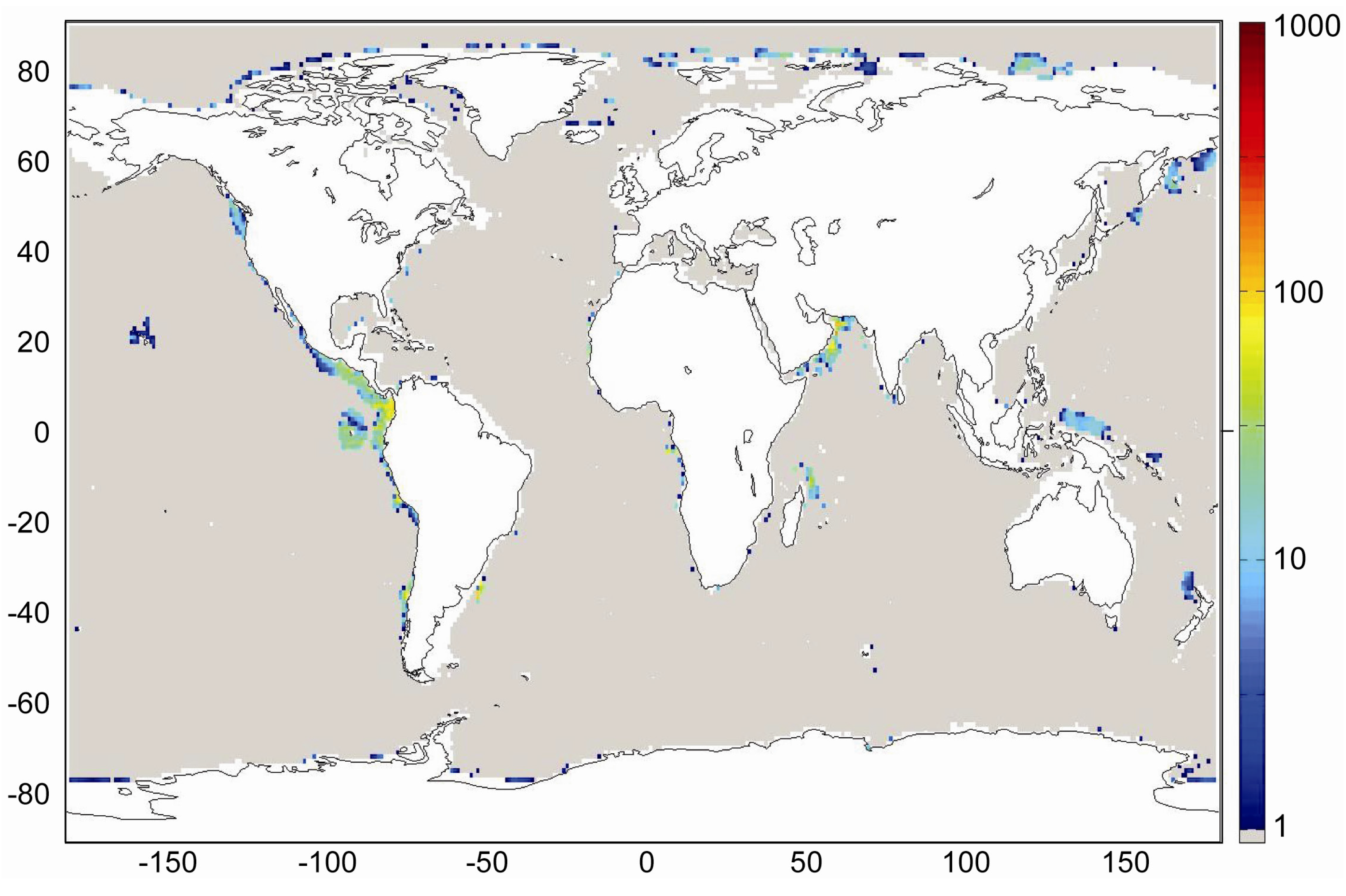
Transfer function Equation (31) which is valid for sediments experiencing a low degree of compaction was applied with Holocene burial velocities to provide a minimum estimate for the accumulation of gas hydrates in marine sediments. The global inventory of methane hydrates in marine sediments amounts to only 3 Gt of C under these boundary conditions. Low-grade gas hydrate occurrences are predicted for some high productivity areas with depth-integrated hydrate inventories of less than 40 kg m⁻². These low values are consistent with the previous model results for Holocene boundary conditions presented by Burwicz et al. [6] yielding a global gas hydrate inventory of only 4 Gt of C.

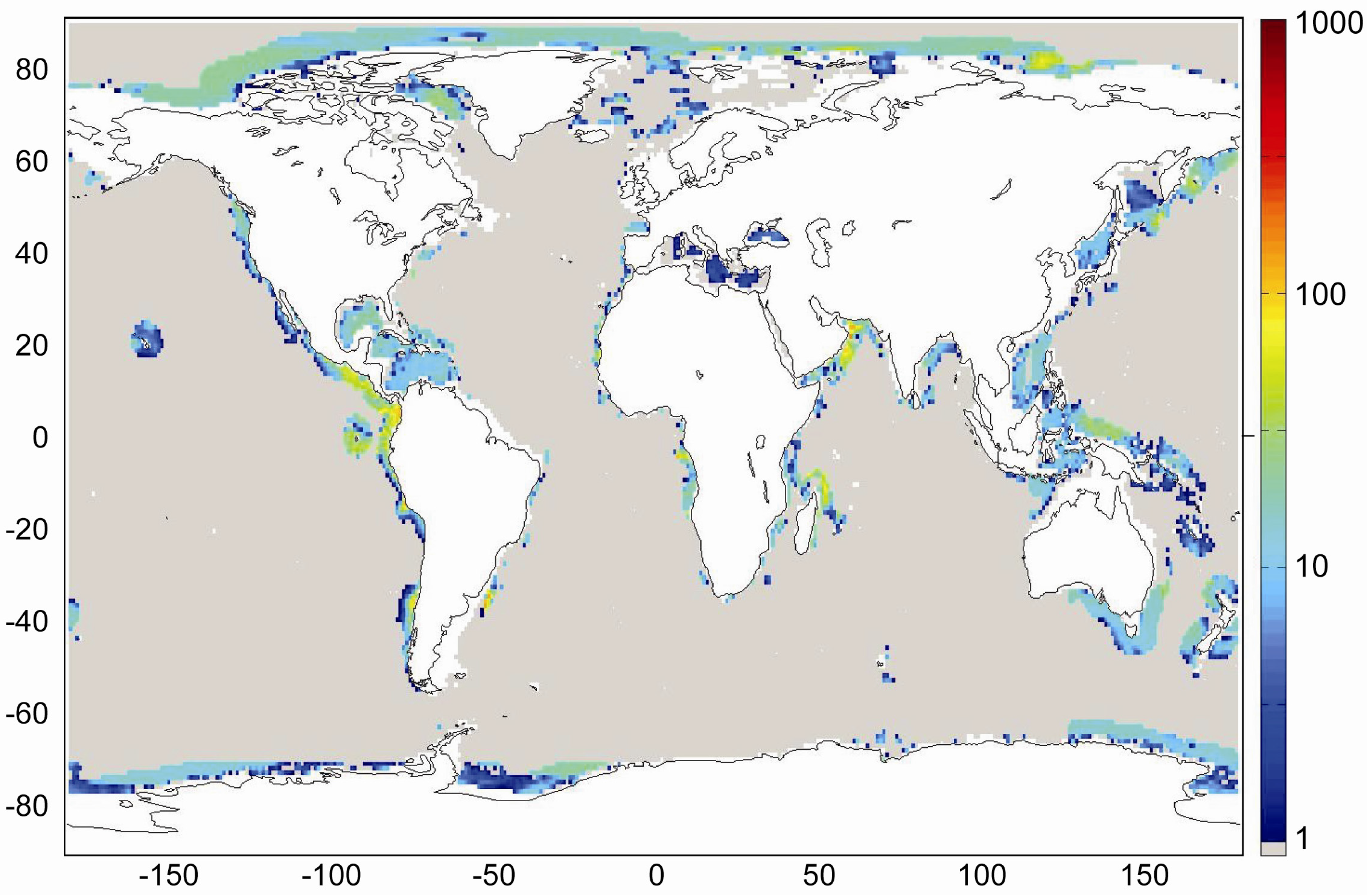
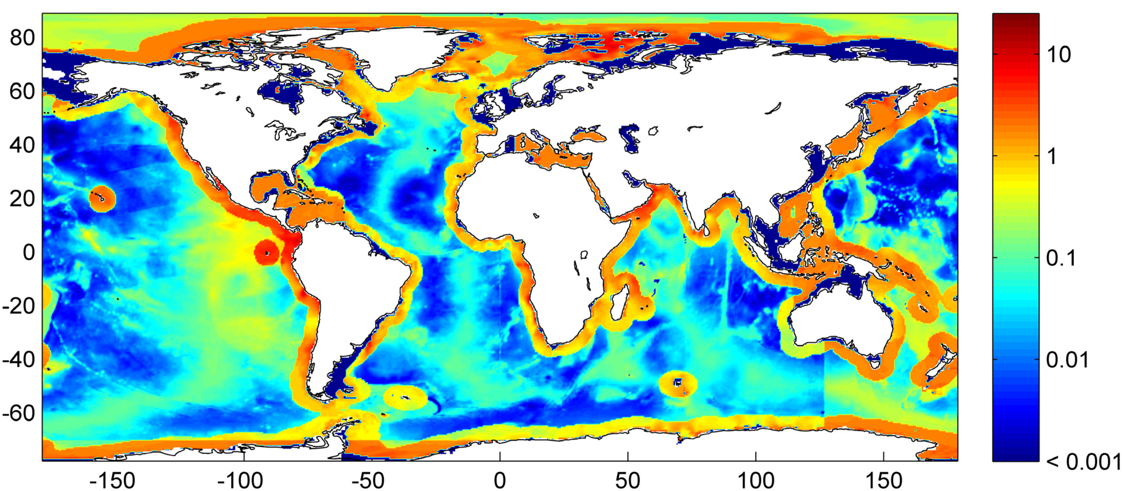
The transfer function valid for low compaction [Equation (31)] was also applied on a grid with Quaternary burial velocities to consider the down-slope transport of sediments during glacial sea-level low-stands (Figure 30). The global inventory of methane hydrates in marine sediments expands to 122 Gt of C due to the increase in burial velocity. The map shows extended hydrate-bearing areas at productive continental margins. Elevated inventories of up to 230 kg m⁻² are found at the highly productive margin off Peru.

Figure 30. Global distribution of methane hydrate in marine sediments. The map was calculated applying low compaction [Equation (31)] and Quaternary burial velocities. The color coding indicates depth-integrated hydrate inventories in kg C m⁻².

Figure 30. Global distribution of methane hydrate in marine sediments. The map was calculated applying low compaction [Equation (31)] and Quaternary burial velocities. The color coding indicates depth-integrated hydrate inventories in kg C m⁻².

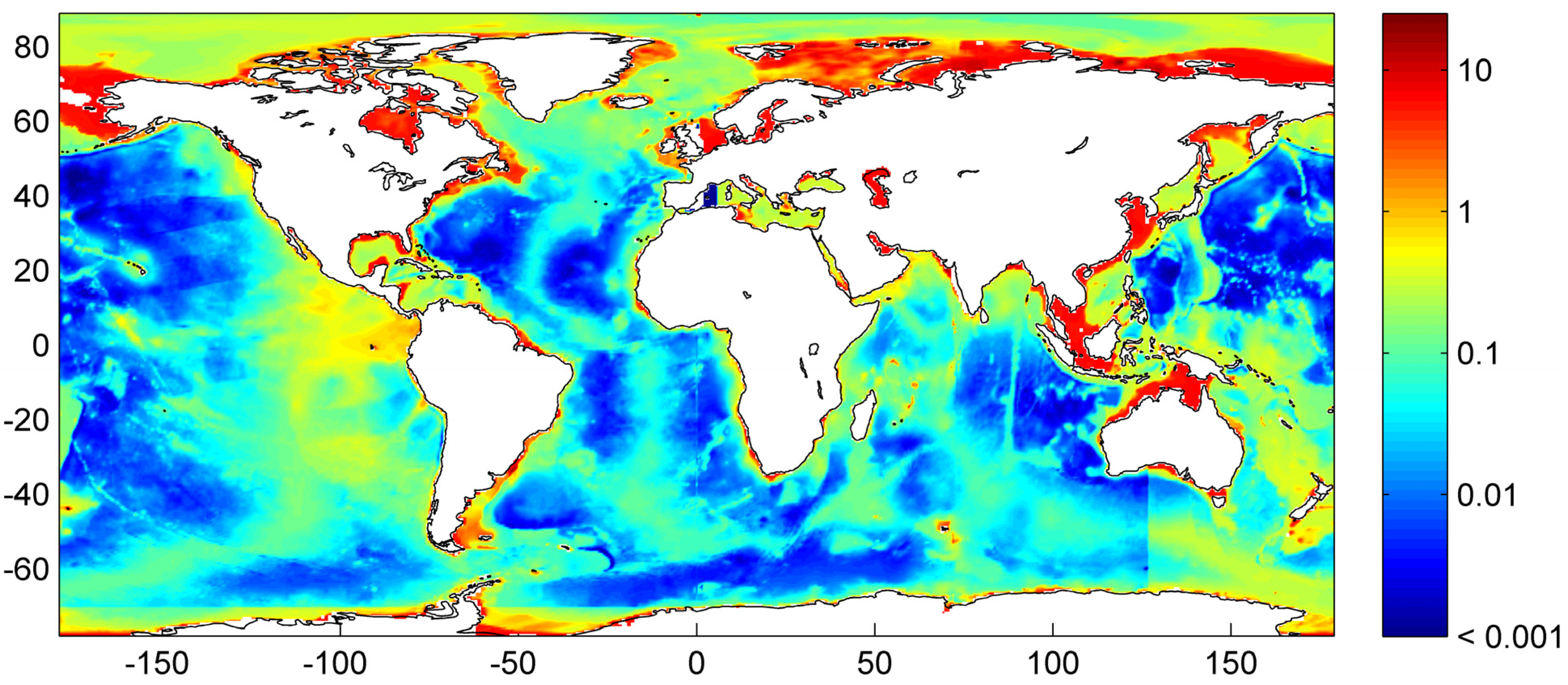
Our best estimate of the global distribution of marine sediments is shown in Figure 31. It is based on the assumptions that margin sediments are completely compacted at large sediment depths and that shelf sediments are eroded and deposited on the continental slope and rise under glacial conditions. The global inventory of gas hydrates derived from our best estimate map (Figure 31) is 455 Gt of C. The map predicts gas hydrate accumulations of ~10 kg m⁻² over extended margin areas with elevated values of >100 kg m⁻² in high productivity zones at the western continental margins and in the Arabian Sea. High values are also calculated at the Argentinean margin and north of Madagascar. The background concentration of methane hydrates in margin sediments of ~10 kg m⁻² corresponds to very low gas hydrate saturations of less than 0.1 Vol.% which are not resolved by geophysical methods and drilling. The true distribution of gas hydrates is probably patchier than the distribution shown in Figure 31 since sediments are not always experiencing full compaction such that dissolved methane is buried and lost below the GHSZ. Fluid flow is implicitly considered in the map since pore fluids are not buried below the GHSZ. This approach is probably valid for passive continental margins. However, it does not consider the additional fluid flow at active margins where pore fluids of the incoming oceanic plate are mobilized and released into the GHSZ. The gas hydrate abundance at active margins is thus systematically underestimated in Figure 31.

Figure 31. Global distribution of methane hydrate in marine sediments. The map was calculated applying complete compaction [Equation (32)] and Quaternary burial velocities. The color coding indicates depth-integrated hydrate inventories in kg C m⁻².

Figure 31. Global distribution of methane hydrate in marine sediments. The map was calculated applying complete compaction [Equation (32)] and Quaternary burial velocities. The color coding indicates depth-integrated hydrate inventories in kg C m⁻².

It should also be noted that steady-state conditions were applied in all model runs. The models were run over a period of several million years until the depth-integrated inventory of gas hydrates reached a constant value. It was assumed that geothermal gradients and POC accumulation rates at the seafloor have been constant over the entire model period. Thus, the model runs do not consider subsidence, thermal evolution and the changes in POC accumulation during basin formation.

Gas ascent and focused fluid flow at active continental margins are not considered in the map. These processes are responsible for the formation of high-grade gas hydrate accumulations which have been documented at an ever increasing number of sites [78,79]. The global picture that emerges from our modeling exercise may be summarized as: Gas hydrates occur at many continental margin sites at very low saturations of less than 0.1%. Higher saturations of 1%–3% appear at productive continental margins where abundant organic matter is delivered to the seabed by the sinking of biogenic detritus. High-grade deposits with saturations of >3% are formed only where fluid and/or gas have migrated into the GHSZ. These deposits are not shown on the map since it is currently not possible to constrain the global distribution of these high-grade gas hydrate deposits.

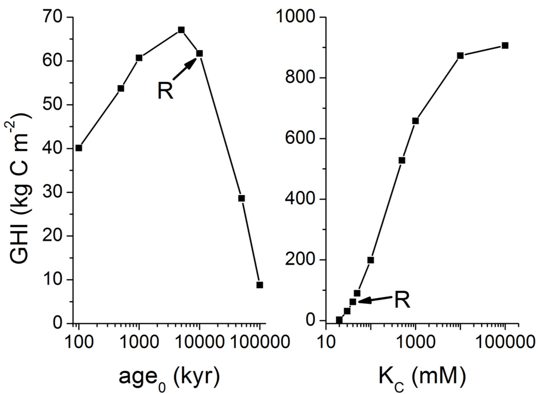
Our estimate of the global abundance of marine gas hydrates is certainly too low since gas ascent and focused fluid flow are not considered. Fluid and gas flow have an enormously strong effect on gas hydrate accumulation. The gas hydrate inventory is enhanced by about two orders magnitude already at very low velocities of fluid and gas ascent (u_w < 2 cm kyr⁻¹; u_G < 0.02 cm kyr⁻¹, s. Figure 25). It is currently not possible to constrain the global number and abundance of these hot spots for gas hydrate accumulation. However, the modeling presented in this contribution suggests that the global inventory of methane in these hot spot areas may exceed the global hydrate inventory of low-grade deposits if only 1% of the global seafloor would be affected by upward gas or fluid flow.

The gas hydrate distribution shown in Figure 31 may be used for prospection purposes while Equation (32) can be applied to estimate the gas hydrate inventory where ambient data for w₀, L_GHSZ and POC₀ are available. It should, however, be noted that detailed local surveys will almost certainly reveal inventories differing considerably from the predicted values since the regional basin evolution and the local pathways for fluid and gas flow are not resolved in our global estimates. Seismic surveys and drilling data are needed to constrain local gas hydrate inventories. Moreover, new 3-D basin modeling tools have recently been developed that can be used to better constrain gas hydrate inventories in well characterized sedimentary basins [80]. These models can be used to simulate in detail the thermal and sedimentary history and the ascent of gas and fluids through faults and fractures at selected sites. However, it will not be possible to apply these basin models at global scale in the foreseeable future.

The first model-based estimate of the global methane hydrate inventory under Holocene boundary conditions was presented by Buffett and Archer [3]. They used the POC rain rate to the seabed as a major external driving force for the simulation of hydrate formation in marine sediments. The rain rate was calculated as a function of water depth and applied as an upper boundary condition for an early diagenesis model simulating the degradation of POC in the top meter of the sediment column [81]. The POC burial rate at 1 m sediment depth calculated with this “muds” model was applied as upper boundary condition for the simulation of methane turnover in the underlying sediment sequence. The later simulations consider the microbial degradation of POC via sulfate reduction and methanogenesis and the anaerobic oxidation of methane within the sulfate-methane transition zone [82,83]. POC was separated into an inert fraction and a labile fraction that was degraded over the top km of the sediment column following first order reaction kinetics (rate constant 3 × 10⁻¹³ s⁻¹). The model also considers an externally imposed rate of upward fluid flow. It was calibrated using field data obtained at Blake Ridge (a passive margin site) and the Cascadia margin (active continental margin). The best fit to observations was obtained assuming that the 25% of the total POC is labile and using upward fluid flow velocities of 0.23 mm yr⁻¹ (passive margin) to 0.4 mm yr⁻¹ (active margin). Applying these parameter values on a global grid and assuming a compensating downward fluid flow over 50% of the global seafloor area resulted in a total methane hydrate inventory of 3000 Gt C. The hydrate inventory was to a large degree controlled by the velocity of upward fluid flow. Without imposed fluid flow, the global hydrate inventory was reduced to 600 Gt C. Subsequently, the authors discovered an extrapolation error in the calculation of POC rain rates as function of water depth [5]. The model-based estimate of the global hydrate inventory was reduced from 3000 Gt C to approximately 700–900 Gt C after correction for this error [5].

Klauda and Sandler [4] used a modified version of the Davie and Buffett model [82,83] to estimate the global marine hydrate inventory under Holocene boundary conditions. The entire POC pool was assumed to be completely degradable with a reduced decay constant of 1.5 × 10⁻¹⁴ s⁻¹. The upper boundary of the model domain was constrained by field data. POC concentrations measured in surface sediments and Holocene sedimentation rates averaged over the major ocean basins were applied to define the POC burial flux at the sediment surface. The global hydrate inventory estimated with this approach was surprisingly high (55–700 Gt C) even though the model was run without imposing upward fluid flow. Unfortunately, Klauda and Sandler [4] did not consider POC degradation via sulfate reduction. The large difference to our estimate may be explained by the neglect of microbial sulfate reduction and AOM since the accumulation of methane in pore fluids and gas hydrates is strongly diminished by these processes.

Burwicz et al. [6] performed the first simulation of gas hydrate formation under Quaternary boundary conditions at global scale. Their estimate of the global gas hydrate inventory in marine sediments (995 Gt C) is larger than our Quaternary estimates for low and complete compaction (122 Gt C and 455 Gt C, respectively). Burwicz et al. [6] applied a different compaction law and assumed very low porosities for GHSZ sediments. Moreover, they used a significantly higher value for the mean thermal conductivity of marine sediments (1.5 W m⁻¹ K⁻¹) resulting in a very strong expansion of the GHSZ with respect to our modeling (s. discussion in section 4). To test the effect of the GHSZ expansion, we applied their GHSZ grid in an additional model run. We obtained a global GHI value of 937 Gt C for Quaternary conditions and full compaction [Equation (32)] which is close to the value derived by Burwicz et al. [6] (995 Gt C). We conclude that the difference between our best estimate (455 Gt C) and the previous estimate (995 Gt C) by Burwicz et al. [6] is mainly caused by the different choice of thermal conductivity values. The maps presented by Burwicz et al. [6] were produced by performing a full-scale 1-D transport-reaction simulation at each grid point. They are thus more precise than our estimates which are affected by additional errors introduced by the transfer functions. However, the available data strongly suggest that the thermal conductivity of most continental margin sediments is smaller than 1.5 W m⁻¹ K⁻¹ and close to the value applied in our modeling (1.0 W m⁻¹ K⁻¹). We thus conclude that the gas hydrate distribution shown in Figure 31 and our new best estimate of the global gas hydrate abundance (455 Gt C) are more realistic than previous results.

9. Accumulation of Gas Hydrates under PETM Boundary Conditions

The strong negative isotopic carbon excursion observed during the PETM (55.5 Ma ago) has been ascribed to the dissociation of methane hydrates in marine sediments [18,84,85]. About 1000 Gt of methane carbon release are required to explain the isotope values observed in marine carbonates. The conditions at the PETM were very different from today. The bottom water temperatures were close to 10 °C, the burial velocities of terrigenous sediments were reduced by a factor of ~4–5 while the POC concentrations in surface sediments were probably much higher than today (Figure 4).

To test the potential for gas hydrate formation prior to onset of the PETM, the standard simulation with full compaction was run at a bottom water temperature of 10 °C, a POC concentration of 4 wt.% and a burial velocity of w₀ = 33.7 cm kyr⁻¹ (Figure 32) The thickness of the GHSZ was reduced to ~265 m due to the elevated bottom water temperature while methane production rates were enhanced due to the increase in POC concentration. The resulting gas hydrate saturation values were similar to the saturations obtained under modern conditions (Figure 32). However, the overall effect was a decrease in the GHI from 99 kg C m⁻² in the modern ocean to 19 kg C m⁻² in the PETM.

Figure 32. Concentrations of dissolved inorganic carbon (DIC), dissolved methane (CH₄), particulate organic carbon (POC) and methane hydrate saturation (GH-Sat.) calculated for the modern ocean and the PETM. The modern ocean simulation was done for the reference case with complete compaction (Φ_f = 0.0, p = 1/1300 m⁻¹). The PETM simulation was based on the reference case with complete compaction applying a bottom water temperature of 10 °C, a POC concentration of POC₀ = 4 wt.% and a reduced burial velocity of w₀ = 33.7 cm kyr⁻¹.

Figure 32. Concentrations of dissolved inorganic carbon (DIC), dissolved methane (CH₄), particulate organic carbon (POC) and methane hydrate saturation (GH-Sat.) calculated for the modern ocean and the PETM. The modern ocean simulation was done for the reference case with complete compaction (Φ_f = 0.0, p = 1/1300 m⁻¹). The PETM simulation was based on the reference case with complete compaction applying a bottom water temperature of 10 °C, a POC concentration of POC₀ = 4 wt.% and a reduced burial velocity of w₀ = 33.7 cm kyr⁻¹.

These model results suggest that the potential for gas hydrate accumulation before the onset of the PETM was lower than today. Wide-spread ascent of pore fluids and/or methane gas into the GHSZ has to be postulated for the period prior to the PETM to explain the isotopic excursion by gas hydrate dissociation.

10. Conclusions and Open Questions

A number of improved global estimates can be derived from the data and model results presented above:

• The global POC accumulation rate in the modern ocean amounts to ~1.4 × 10¹⁴ g yr⁻¹.
• The global rate of microbial methane formation in marine sediments is lower than previously assumed and falls into the range of 4 − 25 × 10¹² g C yr⁻¹.
• The pore volume within the GHSZ is extensive and can be constrained as ≥44 × 10¹⁵ m³.
• The global inventory of methane hydrates in marine sediments is ≥455 Gt C.

The global distribution maps of methane hydrate presented in this contribution are representative for methane hydrate being formed by the microbial degradation of POC within the GHSZ. The maximum pore space saturation reached under these conditions is 3 vol.%. However, sediment cores and logs obtained at an ever growing number of sites have clearly shown that the saturation values are much higher than 3 vol.% under favorable geologic conditions. Our model results clearly show that these highly concentrated gas hydrate deposits have been formed by the migration of dissolved or gaseous methane into the GHSZ. Potentially exploitable gas hydrate reservoirs are thus only formed where gas or water has been transported into the GHSZ via upward advection. Fluid and gas flow have an enormously strong effect on gas hydrate accumulation. The gas hydrate inventory is enhanced by about two orders magnitude already at very low velocities of fluid and gas ascent (u_w < 2 cm kyr⁻¹; u_G < 0.02 cm kyr⁻¹).

The global distribution of methane hydrates is probably characterized by the wide-spread occurrence of low-grade hydrate saturations (<0.1 vol.%) along continental margins superimposed by elevated saturations in highly productive regions (1–3 vol.%). Observational data reveal a large number of “sweet spots” where saturations are enhanced by methane migration (>3 vol.%). However, it is currently not possible to constrain the global number and abundance of these high-grade deposits by numerical modeling.

The Quaternary is characterized by very low bottom water temperatures and extremely high rates of POC accumulation at the seabed. It offers unusually favorable conditions for gas hydrate accumulation since the inventory of gas hydrates in marine sediments increases under low temperature and high POC input. The conditions were much less favorable during most of the Cenozoic and Cretaceous. This is also true for the PETM where large-scale gas hydrate dissociation has been evoked to explain a global negative excursion observed in the δ¹³C record. Thus, wide-spread ascent of pore fluids and/or methane gas into the GHSZ has to be postulated for the period prior to the PETM to explain the isotopic excursion by large-scale gas hydrate dissociation.

More work is needed to better constrain the global gas hydrate inventory in the seabed. This work should address at least some of the following open questions:

• What are the major geochemical and biological control mechanisms regulating the rate of microbial methane production in the deep biosphere?
• What precisely are the physical and geological controls on gas transport into the GHSZ? Is gas ascending into the GHSZ already at low gas saturation values? What defines the critical gas saturation value that needs to be overcome to allow for gas migration?
• What fraction of the global seabed is affected by upward gas and fluid flow?
• How does the hydrate inventory evolve under non-steady state conditions?