Article

A Spinning Reserve Allocation Method for Power Generation Dispatch Accommodating Large-Scale Wind Power Integration

Department of Electrical Engineering, Tsinghua University, Haidian District, Beijing 100084, China
*
Author to whom correspondence should be addressed.
Energies 2013, 6(10), 5357-5381; https://doi.org/10.3390/en6105357
Submission received: 28 August 2013 / Revised: 8 October 2013 / Accepted: 10 October 2013 / Published: 18 October 2013

Abstract

:
Spinning reserve allocation is a critical problem for active power dispatch with large-scale wind power penetration. A risk-based reserve allocation method that accounts multiple control sub-area coordination is given in this paper. And a multi-objective optimization model is constructed to schedule the spinning generation reserve for online active power dispatch. A fuzzy optimization method is used to transform the multi-objective optimization problem into a single-objective optimization one. The relationship between loss of load expectation and spinning reserve is also derived. And a particle swarm optimization (PSO) method is employed to provide a numerical solution to the problem. Numerical tests on IEEE RTS system are also given to validate the proposed method.

1. Introduction

Wind power generation is one of the most important renewable energy forms and it has seen an ever-increasing development in the past decades all over the World, but especially in China, which has now the largest wind turbine installation capacity in the World. The installed wind turbine capacity in China had reached 62,660 MW by the end of 2012 and is still developing fast. However, despite its benefits of low operating cost and low pollutants emission, large-scale wind power generation introduces great technical challenges for power systems because of its intrinsic intermittent and fluctuant output characteristics. In particular, due to its limited predictability of wind power, the operational reliability cannot be guaranteed with the conventional deterministic spinning reserve method, and extra spinning generation reserves are needed to accommodate wind power integration [3,4].
Power generation reserves can be classified into spinning reserves and non-spinning reserves according to the North American Electric Reliability Corporation (NERC) definitions [5]. In China, the power generation reserves are divided into load following reserves, contingency reserves and maintenance reserves, where the load following and contingency reserves constitute the spinning reserves, and the maintenance reserves constitute the non-spinning reserves, which are used for different time-scale power generation dispatch and control [6]. In the past several years, much research has been done to evaluate the spinning reserve requirements of systems with high wind power penetration. A multi-time-scale reserve power dispatch method [6] and reserve allocation method [7] are proposed to accommodate the integration of wind power generation. Lee [8] presented an evolutionary iteration particle swarm optimization algorithm for spinning reserve optimization of a wind-thermal power system, in which the outage cost as well as the total operation cost of thermal units is considered to evaluate the spinning reserve capacity. In reference [9], a cost-benefit analysis, which takes the outage cost into account, is presented for spinning reserve optimization to achieve a better economical balance. Reference [10] presents a load shedding probability index which takes the wind power uncertainty into account, and the system reliability is used as the measure for the influence of wind power penetration. In [11], a risk reserve constraint-based dynamic economic dispatch model is given, which schedules wind power under the restraint of the given risk threshold. In [12], the reserve cost is considered in the objective which is comprised of the penalty cost of underestimation and the reserve cost of overestimation of the available wind power. Morales et al. [13] proposes a stochastic programming model for spinning reserve optimization in the power system with high wind power penetration, in which both load shedding cost and wind spillage cost are accounted.
Although much work has been done on spinning reserve optimization, most of these studies are focused on evaluating the spinning reserve capacity requirements, and only a little work pays attention to the spinning reserve allocation problem for a reliable operation of multi-area power system [14,15]. In fact, with large-scale wind power penetration, the power flow fluctuates intensively and drastically, making the transmission interface easily heavy or over loaded, which brings more pressure on the transmission interfaces [16]. A limited transmission interface capacity may mean more localized reserve requirements. In such cases, a not well-optimized spinning reserve allocation result for a multi-subarea system may make the inter-zonal reserve supplies constrained by the transmission interface limits, resulting to the consequence of local reserve inadequacy and transmission interface overload, which could seriously damage the operational security of the power system [17]. Thus, the spinning reserve allocation problem becomes especially serious for the grids with large-scale wind power integration. Reference [14] presents a model which includes area demand constraints, area reserve constraints and tie line capacity constraints between the modeled areas, for solving the multi-area economic dispatch problem with tie line constraints. Ref. [15] presents a LP-based joint dispatch approach, which dispatches energy and reserve market concurrently, for solving the multi-product, multi-zone/area physical market dispatch problem. However, the wind power characteristics are not taken into account in the above two references and thus they are only suitable for conventional power grids with no wind power penetration. For the power grid with large-scale wind power integration, the uncertainty characteristic of wind power output has to be considered and a probability-based method is required for this.
In this paper, the spinning reserve allocation problem of a multi-subarea system is investigated for active power generation dispatch. A risk-based multi-objective spinning reserve optimization model, which considers the coordination of multiple control subareas, is proposed. The relationship between loss of load expectation (LOLE) and spinning reserve is also derived. The fuzzy optimization and particle swarm optimization methods are used for this multi-objective optimization model.
This paper is organized as follows: the spinning reserve allocation optimization model for active power dispatch considering operational risk, penalty cost of wind power curtailment and power production cost is proposed in Section 2, and the fuzzy optimization is applied for this model. Then the relationship between loss of load expectation (LOLE) and spinning reserve is derived in Section 3. Section 4 describes the calculation procedure of the reserve capacity for a multiple sub-area system. Next, a PSO-based method is applied for the optimization of the proposed model in Section 5. Numerical results on the IEEE RTS system are given in Section 6. Finally, some conclusions are drawn in Section 7.

2. Problem Modeling

2.1. Proposed Model

A well scheduled multi-subarea spinning reserve allocation result should effectively handle the problem of local reserve inadequacy and transmission interface overload. Hence, a risk sharing principle is applied in the proposed spinning reserve allocation method, which means that the operational risk is shared evenly by all the subareas, to avoid the possibility of a large blackout or wind power curtailment. And a reserve balance index I t with the variance form, which is widely applied for risk management in finance and electricity market [18,19,20], is defined as follows to evaluate the degree of operational risk differences among multi-subareas:
I t = 1 n j = 1 n ( r j t r ¯ t ) 2
where, r j t = E G j t D j t .
The variance index was first used to represent the risk by Markowitz, who in 1952 defined risk as the volatility of expected return. When the variance becomes smaller, the data sequence becomes more stable, which means a lower risk for the investment process. What is sought in the process is the benefit maximization under certain risk levels or the risk minimization under some expected benefit levels. As the subareas may have quite different load demand levels, the same amount of load losses may be disastrous for a small subarea, while it is only a very small portion for a large subarea. Hence, a normalized operation on LOLE is necessary for risk evaluation among subareas. When I t gets smaller, the running risk gets more balanced and the possibility of a large local blackout or wind power curtailment gets lower, and vice versa.
Meanwhile, the economic and environmental considerations are another two primary factors in determining the unit output during the active power dispatch process. Therefore, the spinning reserve allocation problem is essentially a multi-objective optimization problem which can be formulated as follows:
(1) Objective
The objective of the spinning reserve allocation model can be expressed as follows:
{ f 1 = j G w i n d t = t 0 + 1 T λ j ( p j t f p j t w ) f 2 = i = 1 N t = t 0 + 1 T ( a i p i t 2 + b i p i t + c i ) f 3 = t = t 0 + 1 T I t          
where p j t f    can be obtained from Numerical Weather Prediction (NWP) model or statistical model like the persistence method depending on the actual conditions of the wind farms. And λ j > 0 must be satisfied to achieve the objective of a minimum possibility of wind power curtailment, which can be deduced from the equal incremental principle.
(2) Constraints
① LOLE threshold constraint
From the operational reliability aspect, a certain amount of spinning reserve must be reserved in advance. This is achieved by Equation (3):
E t E t h r e s h
where the expression of E t will be given in Section 3, and E t h r e s h is usually specified by the operators [21]. From the mathematical optimization aspect, constraint (3) becomes looser when E t h r e s h becomes larger, and the objective of the model becomes smaller, and vice versa. In fact, this reflects the tradeoff between security and economics of the power grid. And when E t h r e s h is small enough, there can be no solution for the model. Hence, a pre-calculation of minimum E t h r e s h can be done by setting E t as the objective instead of Equation (2) if needed.
② Active power balance constraint
The power balance between active power generation and load demand must be kept all the time during the normal operation status of the power system, which can be expressed by Equation (4), in which the power losses are neglected:
i = 1 N p i t + j G wind p j t w = D t
where Dt can be obtained from linear extrapolation method for short term time periods and its prediction technology is relatively mature now.
③ Unit capacity constraint
The following inequalities should be satisfied:
p i _ p i t p ¯ i   
0 p j t w p j t max                   j G w i n d
where, p j t max should be greater than p j t f with the prediction error considered.
④ Ramp rate constraint for conventional units
p i , t 1 Δ p d i T 15 p i t p i , t 1 + Δ p u i T 15   
where T 15 is adopted in this paper according to the operating rules of China’s power grid [22]. Even if the operating rules are different for other power grids [23], the parameter can be easily adjusted.
⑤ Spinning reserve definition
R i t u = min ( Δ p u i T 10 , p ¯ i p i t )
R i t d = min ( Δ p d i T 10 , p i t p _ i )
R t u = i G wind R i t u
R t d = i G wind R i t d
⑥ Transmission interface capacity constraint
T L l _ i = 1 N ( k l i p i t ) + j G w i n d ( k l j p j t w ) T L l ¯ , l = 1 , , L
It can be seen from Equation (2) to Equation (12) that the proposed model is an operational-reliability-constrained [Equation (3)] risk-sharing optimization model, which is also a multi-objective optimization model. For this type of optimization problem, the traditional multi-objective weighting method is often used, but the values of the weight coefficients, which have a significant impact on the results, are difficult to determine, hence, the fuzzy optimization method, which is well capable of tackling multi-objective optimization problems with disparate and contradicting objectives [2], is used for this model to transform the multi-objective optimization problem into a single-objective optimization problem which can be easily solved.

2.2. Fuzzy Optimization-Based Multi-Area Reserve Allocation Model

The fuzzy optimization method, which provides an excellent mathematical treatment for multi-objective optimization problems, has been widely used in the literature for large multi-objective optimization challenges [2,24,25]. With the introduction of membership function, the fuzzy optimization method can transform the optimization model into a single-objective optimization problem with the original constraints and an objective to maximize the minimum of such membership function. A satisfactory number of multiple contradictory objectives can be simultaneously considered in the optimization problem. The “best” compromised solution among the Pareto-optimal solutions of the multi-objective optimization problem can be obtained with this method [26].
For the proposed reserve allocation model, the membership function for the penalty cost of wind power curtailment can be formulated as Equation (13) and is plotted in Figure 1.
μ 1 = e ( p w p f σ ) 2
Figure 1. Membership function for the penalty cost of wind power curtailment.
Energies 06 05357 g001
As both the production cost f 2 and the operating risk f 3 are required to be as small as possible, a monotonically decreasing quadratic polynomial membership function is adopted as follows to reflect the operator’s attitude towards security and economics of the system, and its shape is shown in Figure 2:
μ 2 = α 1 f 2 2 + β 1 f 2 + γ 1
μ 3 = α 2 f 3 2 + β 2 f 3 + γ 2
where, α 1 , β 1 , γ 1 and α 2 , β 2 , γ 2 can be obtained from equation μ i ( f i , min ) = 1 and μ i ( f i , max ) = 0 . The results are as follows:
α i = 2 k i ( f i , min f i , max ) 2 , β i = 1 f i , min f i , max α i ( f i , min + f i , max ) , γ i = f i , max f i , min f i , max + α i f i , min f i , max
where k i [ 1 , 1 ] and its value plays a major role on the shape of the membership function as shown in Figure 2 k i > 0 represents a pessimistic attitude towards the relevant objective and the optimization tends to decrease the corresponding objective value; while k i < 0 represents an optimistic attitude towards the corresponding objective. The values of coefficient k i for different objectives define the compromise degree between economics and security. For example, if the operating cost is what to be more pursued, then a larger positive value should be taken for k1. Otherwise, if the operational risk is emphasized more, then a larger positive value should be set for k 2 . Especially, k i = 0 stands for a neutral attitude to the relevant objective, and with this k i value, the membership functions (14) and (15) can be simplified as:
μ 2 = f 2 , max f 2 f 2 , max f 2 , min
μ 3 = f 3 , max f 3 f 3 , max f 3 , min
Figure 2. Membership functions with different k values.
Energies 06 05357 g002
It can be seen that the membership function approaches its maximum value 1 when the corresponding objective reaches its minimum value, and the membership function gets its minimum value 0 when the optimization objective reaches its maximum value. Therefore, the optimization result becomes better when the membership function gets larger, and vice versa. With the above definition of the membership function, the original multi-objective optimization problem can be transformed into a single objective optimization model as shown in Equation (19):
{ max      λ                                                                                                               s . t .       μ 1 = e ( p w p f σ ) 2 λ                               μ 2 = α 1 f 2 2 + β 1 f 2 + γ 1 λ                          μ 3 = α 2 f 3 2 + β 2 f 3 + γ 2 λ                            0 λ 1 ( 3 ) ( 12 )                                                        

3. Relationship between LOLE and Spinning Reserve
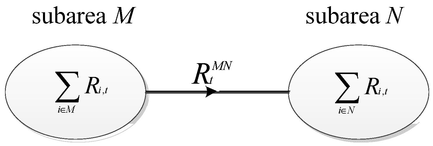
One of the key problems for the proposed optimization model is how to derive the expression for LOLE. In this section, the relationship between spinning reserve and LOLE is investigated considering wind power integration.
For the power system penetrated with wind power, the contingency considered for LOLE should include forced outages of generators and predicted errors of load demand and wind power. Generally, more than triple generator failures are negligible as their probability is very small. Hence, only three scenarios are considered for LOLE calculation: (1) No generator outage and only the predicted error of load demand and wind power are accounted; (2) one generator outage, with the predicted error of load demand and wind power accounted; (3) two generators outage, with the predicted error of load demand and wind power accounted. The corresponding expressions for LOLE in these scenarios are derived as follows:
(1) For the scenario of no generator outage, only the predicted error of wind power and load demand are accounted for LOLE calculation:
E 1 t = i = 1 G ( 1 F O R i , t ) R t ( x R t ) f ( x ) d x = σ t i = 1 G ( 1 F O R i , t ) R t / σ t ( x σ t R t σ t ) 1 2 π e 1 2 ( x σ t ) 2 d ( x σ t )
As the predicted error variable x only takes the value larger than Rt in Equation (20), the integral of x R t gives the reserve inadequacy expectation. Meantime, the product 1 F O R i , t gives the probability of no generator outage. Hence, E 1 t gives the LOLE with no generator outage. It can be seen that Equation (20) is only correlated with the variable Rt after integral. When Rt becomes larger, E 1 t becomes lower. And this is also applicable for Equations (22) and (23), which means more reserve, less risk in the power system.
It is indicated from the statistical data of wind power output that the wind power prediction error gets larger when the forecast period becomes further, and it approximately follows a β distribution for a specific area [27]. However, there is generally a wide geographical expansion for large-scale wind farms with numerous wind turbines, so their output usually follows a normal distribution according to the central-limit theorem. Hence, a normal distribution with mean 0 and standard deviation σ 1 ( t ) is assumed for wind power forecast error in this paper. And load forecast error can also be formulated as a normal distribution with standard deviation σ 2 ( t ) . As wind power and load demand forecast errors are usually considered uncorrelated, the sum of the standard deviation of the two forecast errors can be expressed as σ t = σ 1 2 ( t ) + σ 2 2 ( t ) .
Meanwhile, the instantaneous forced outage rate for a unit during time period t can be expressed as [28]:
F O R ( t ) = λ λ + μ + e ( λ + μ ) t λ + μ [ μ U ( 0 ) λ A ( 0 ) ]
where A(0) and U(0) are the status of the unit during the initial time period. And if it is on, A(0) = 1, U(0) = 0, and vice versa. Obviously the steady-state forced outage rate is F O R ( t ) = t λ / ( λ + μ ) .
Let y = x σ t , then y will also follow normal distribution, and Equation (20) can be simplified as:
E 1 t = σ t i = 1 G ( 1 F O R i , t ) R t σ t ( y R t σ t ) 1 2 π e 1 2 y 2 d y = i = 1 G ( 1 F O R i , t ) ( σ t 2 π e 1 2 ( R t σ t ) 2 R t Q ( R t σ t ) )
where Q function is defined as:
Q ( X ) = X 1 2 π e 0.5 x 2 d x
The LOLE expressions for the other two scenarios can be derived in a similar way and are described as follows.
(2) For the scenario of one unit outage, LOLE can be expressed as follows:
E 2 t = i = 1 G ( F O R i , t × j = 1 j i G ( 1 F O R j , t ) × R t P i , t R i , t ( x R t + P i , t + R i , t ) f ( x ) d x ) = i = 1 G ( F O R i , t × j = 1 j i G ( 1 F O R j , t ) × ( σ t 2 π e 1 2 ( R t P i , t R i , t σ t ) 2 ( R t P i , t R i , t ) Q ( R t P i , t R i , t σ t ) ) )
Similar to Equation (20), the integral of x R t + P i , t + R i , t gives the reserve inadequacy expectation with one unit outage. Meantime, the product F O R i , t × j = 1 j i G ( 1 F O R j , t ) gives the probability of one unit outage. Hence, E 2 t gives the LOLE with one unit outage. Meanwhile, it can be seen that Equation (22) is not only correlated with the variable Rt, but also correlated with P i , t and R i , t .
(3) For the scenario of two units outage, LOLE can be expressed as follows:
E 3 t = i = 1 G j = 1 j i G ( F O R i , t × F O R j , t × k = 1 k i k j G ( 1 F O R k , t ) × R t P i , t P j , t R i , t R j , t ( x R t + P i , t + R i , t + P j , t + R j , t ) f ( x ) d x ) = i = 1 G j = 1 j i G ( F O R i , t × F O R j , t × k = 1 k i k j G ( 1 F O R k , t ) × ( σ t 2 π e 1 2 ( R t P i , t R i , t P j , t R j , t σ t ) 2 ( R t P i , t R i , t P j , t R j , t ) Q ( R t P i , t R i , t P j , t R j , t σ t ) ) )
Similar to Equation (20), the integral of x R t + P i , t + R i , t + P j , t + R j , t gives the reserve inadequacy expectation with two units outage. Meantime, the product
F O R i , t × F O R j , t × k = 1 k i k j G ( 1 F O R k , t )
gives the probability of two units outage. Hence, E 3 t gives the LOLE with two units outage.
Summarizing the above three scenarios together, the overall LOLE expression can be obtained, which is required in the former part to formulate constraint (3) and objective I t . Meanwhile, it can be seen from the expression that the optimization model is a non-linear and non-convex one, from which only a sub-optimal solution can be obtained with state-of-the-art technology.
The above three scenarios have covered most of the operating states of the system. If higher-order outages need to be considered, a fast sorting method [29] can be used to rank the probability of failure. And the first k failures with relatively high probabilities can then be selected and their corresponding impact on LOLE can be derived in a similar way.
Taken the above LOLE expression of Equations (21)–(23) into μ 3 and Equation (3) of the spinning reserve allocation optimization model (19), an explicit joint optimization model for the active power schedule Pi,t and reserve Ri,t can be formulated. For this model, the particle swarm optimization method depicted in Section 5 is used, with which the optimum reserve allocation results can then be obtained.

4. Calculation of R t for Multi-Sub-Area System

When there are multiple sub-areas in the system, Rt for each sub-area will take a different form as the inter-zonal supplies of reserve may be constrained by the transmission interface limits. To illustrate this, a two sub-area system shown in Figure 3 is used as the example.
Figure 3. Two sub-area example for R t calculation.
Energies 06 05357 g003
In Figure 3, R t M N should satisfy the following constraints:
T L l t _ T L l t R t M N T L l t ¯ T L l t
i N R i , t R t M N i M R i , t
If we denote R t for sub-area M and sub-area N respectively as R t M , and R t N then:
R t M = i M R i , t R t M N , R t N = i N R i , t + R t M N
What should be noted is that R t is different in Equations (21)–(23) as R t M N is different under different circumstances. If two different outage events with units i and j occur in sub-area M and sub-area N, respectively, LOLE for these two sub-areas can be respectively expressed as follows:
E t M = F O R i , t × F O R j , t × k = 1 k i k j G ( 1 F O R k , t ) × R t M P i , t R i , t ( x R t M + P i , t + R i , t ) f ( x ) d x
E t N = F O R i , t × F O R j , t × k = 1 k i k j G ( 1 F O R k , t ) × R t N P j , t R j , t ( x R t N + P j , t + R j , t ) f ( x ) d x
It can be seen that the only difference between Equations (27), (28) and (23) is that P j , t and R j , t disappear in Equation (27) and R t is replaced with R t M . Meanwhile, P i , t and R i , t are absent in Equation (28) and R t is replaced with R t N . The LOLE expressions for scenarios of more than two sub-areas can be derived in a similar way.

5. Solution

The proposed spinning reserve allocation model (19) is hard to solve by conventional mathematical programming algorithms as its constraints are nonlinearly coupled and not continuously differentiable. Hence, a particle swarm optimization method, which doesn’t presuppose any conditions for the model and no approximations and limitations are required for the characteristic of the objective function and search space, is used in this paper. The particle swarm optimization, first proposed by Kennedy and Eberhart [30,31], is a population-based optimization method which can generate a high-quality solution within shorter computation time and exhibits a more stable convergence characteristic than other stochastic methods [8,32,33,34]. Due to the relative simplicity, faster convergence and less strict requirements for parameter tuning, PSO has been successfully applied to various fields of power system optimization such as optimal power flow [35], economic dispatch [36,37,38] and reactive power and voltage control [39]. The main procedure of this algorithm is described as follows:
(1) With the position of the particle swarm as the generator output, and the velocity of the particle swarm as the adjustment, the following matrix is stochastically generated as the initial value of the particle swarm:
Energies 06 05357 i001
A step-by-step initialization is adopted in the procedure to account for the ramp rate constraint of the generator output between any two consecutive time intervals. For the individual j of particle i, the following formula is used to generate its position during time period t:
x i j t = ( P ¯ i , t P _ i , t ) * r a n d ( ) + P _ i , t
where P ¯ i , t = min (    p ¯ i ,     p i , t 1 + Δ p u i T 15 ) , P _ i , t = max ( p _ i , p i , t 1 Δ p d i T 15 ) .
(2) The fitness function for every particle is then calculated. For the equality constraints like g ( x ) = b the following penalty function is adopted:
i = 1 n [ γ i ( g i ( x ) b i ) 2 ]
And for the inequality constraints like h ( x ) 0 the following penalty function is used:
j = 1 m [ ζ j max ( h j ( x ) , 0 ) 2 ]
Adding the above two penalty functions into the objective yields the final optimization objective:
min        ( λ + i = 1 n [ γ i ( g i ( x ) b i ) 2 ] + j = 1 m [ ζ j max ( h j ( x ) , 0 ) 2 ] )
in which the loss of load expectation is calculated according to Equations (21)–(23).
(3) The best fitness position for particle i is calculated as follows:
p b e s t i ( k + 1 ) = { p b e s t i ( k )          f ( x i ( k + 1 ) ) f ( x i ( k ) ) x i ( k + 1 )              f ( x i ( k + 1 ) ) < f ( x i ( k ) )
(4) The global optimal position is calculated for the whole particle swarm:
G b e s t ( k + 1 ) = { p b e s t i ( k + 1 ) | f ( p b e s t i ( k + 1 ) ) = min ( f ( p b e s t j ( k + 1 ) ) ) , j = 1 N }
(5) The correction terms are calculated during this step for the position and velocity of particle, i.e.:
v i j ( k + 1 ) = ω v i j ( k ) + c 1 * r a n d 1 ( ) * ( P b e s t i ( k ) x i j ( k ) ) + c 2 * r a n d 2 ( ) * ( G b e s t ( k ) x i j ( k ) ) x i j ( k + 1 ) = x i j ( k ) + v i j ( k + 1 )
where, ω = ω max ω max ω min k max k [31]; ωmax and ωmin are commonly set to 0.9 and 0.4 respectively; c 1 c 2 represents respectively the impact of the local best and the global best position on the individual particles in the swarm.
(6) When the solution variation in K consecutive iterations is less than the given threshold or the maximum iteration number has been reached, the iteration terminates. Otherwise, returning to step (3) for the next iteration. Taken the obtained global optimal position G b e s t ( k ) back into the equality constraints such as the power balance constraint (4) and the inequality constraints like constraints (3) and (5)–(12), the feasibility of the solution can be checked. And if it is not satisfied, go back to step (1) to repeat the iteration.

6. Numerical Tests

The IEEE RTS system is used in this part as the test system to validate the proposed model, in which the units with the same type and on the same bus are merged as shown in Figure A1. The unit parameters are listed in Table A1 and unit #14 is set to be a wind farm with 700 MW capacity. The wind prediction error follows the normal distribution with mean 0 and standard deviation ( 0.044 + 0.006 t ) p j t f .
The load forecast error also follows the normal distribution with mean 0 and standard deviation 2% of the predicted value. The failure rate for generator i is 0.005–0.0045i/13, and the threshold value for load shedding due to reserve inadequacy is LSI (load shedding incidents) = 4. The ramp rate for thermal units is set to 2% of the unit capacity. The load and wind forecast values are respectively shown in Table 1 and Table 2. Each time interval is 15 min and the optimization horizon is 4 h.
Table 1. Predicted load demand data.
Time period (15 min)Predicted power (MW)Time period (15 min)Predicted power (MW)
11484.0691734.43
21493.61101784.04
31504.83111824.07
41536.02121904.01
51559.23131972.80
61582.43141991.22
71596.01152006.43
81669.64162008.02
Table 2. Predicted wind power output data.
Time period (15 min)Predicted power (MW)Time period (15 min)Predicted power (MW)
1697.969555.42
2670.9610613.92
3522.1611628.79
4431.9712651.96
5418.9613665.66
6421.4914700.00
7432.8015681.85
8450.1416636.93

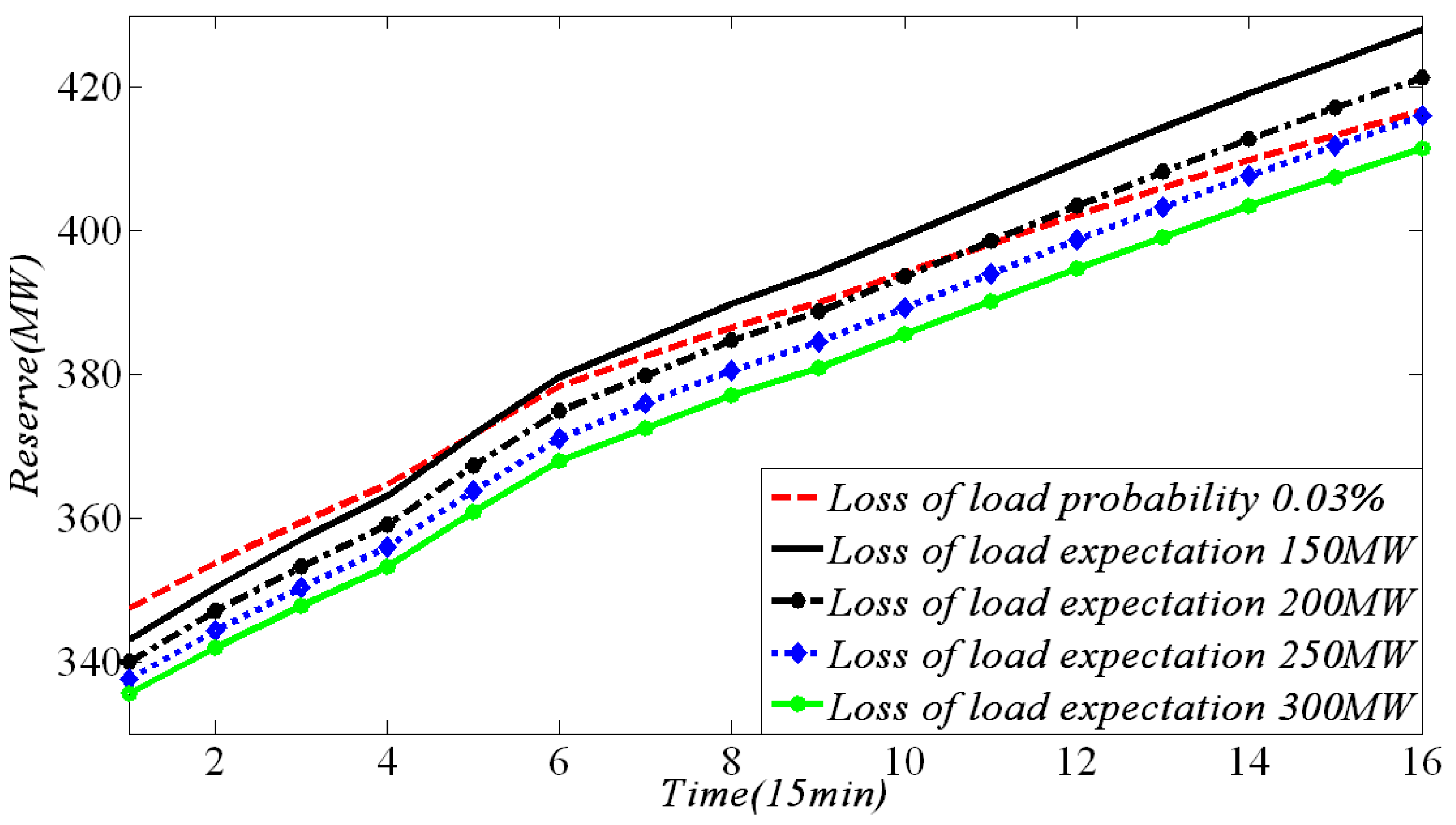
6.1. Relationship between Reserve Capacity and LOLE

Taken the units’ output fixed to their initial values, the reserve demand under different LOLE and LOLP (loss of load probability) values are shown in Figure 4. It can be seen that the reserve demand increases with time, which is mainly due to the time-increasing characteristics of the wind forecast error and the forced outage rate of units. The gradient of the reserve demand curve with LOLP index is smaller than that with LOLE index with time increases. Meantime, when LOLE decreases, and the reserve demand increases correspondingly.
The relationship between the reserve and LOLP/LOLE during the 16th time period is shown in Figure 5.
It can be seen from Figure 5 that when LOLE decreases, the gradient of the curve is correspondingly reduced, indicating a varying important degree of the reserve capacity on system security. When the security level is low, the reserve has a relatively larger effect on the system, and a remarkable improvement of the system reliability would be seen with only a small reserve increase. This effect is weakened when the security level is relatively high. However, the relationship between the reserve and LOLP is approximately linear in this regime. Therefore, it can be concluded that LOLE is a better index for system reliability than LOLP in this respect.
Figure 4. Relationship between the reserve and LOLE/LOLP.
Energies 06 05357 g004
Figure 5. Relationship between reserve and loss of load probability and expectation.
Energies 06 05357 g005

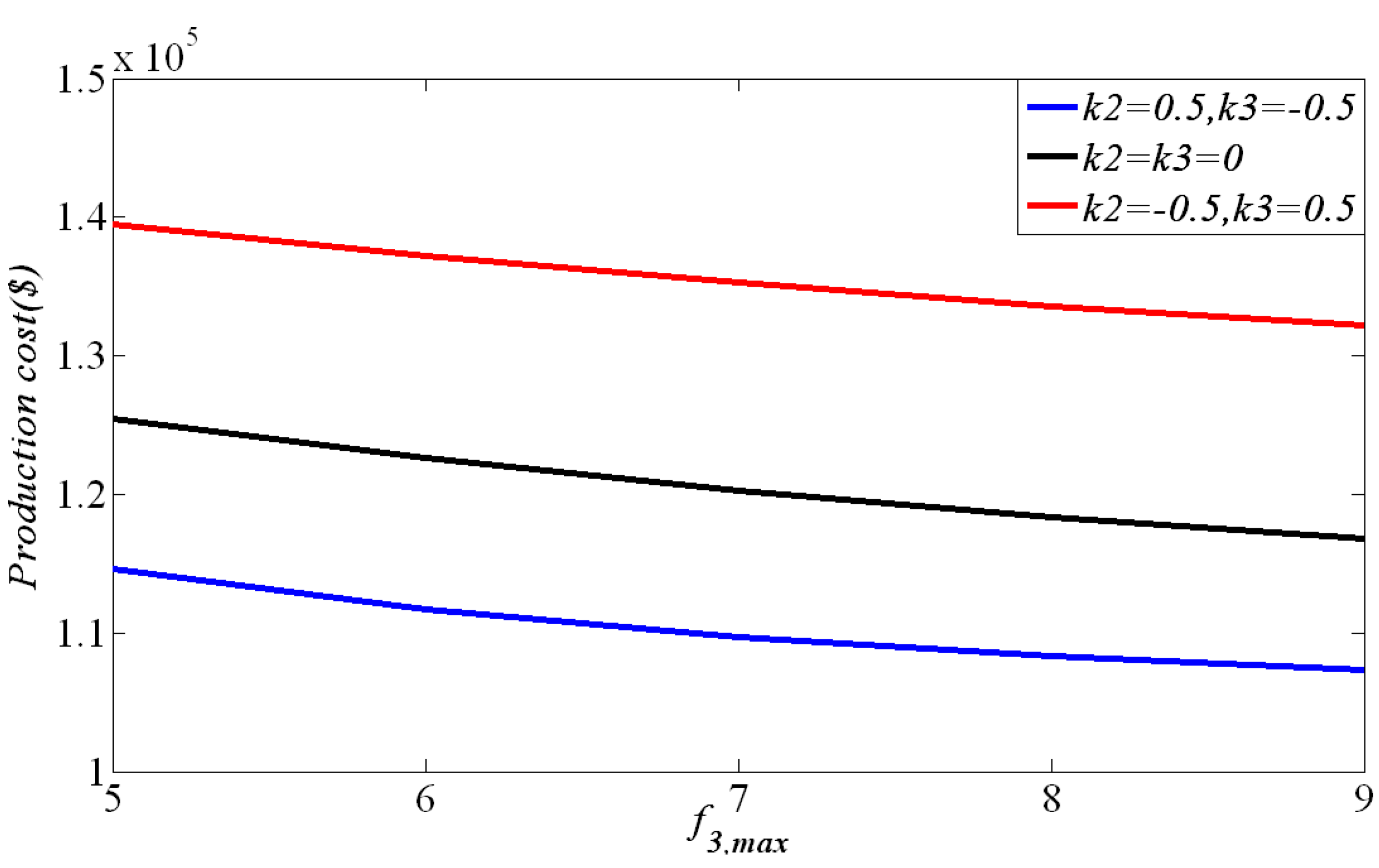
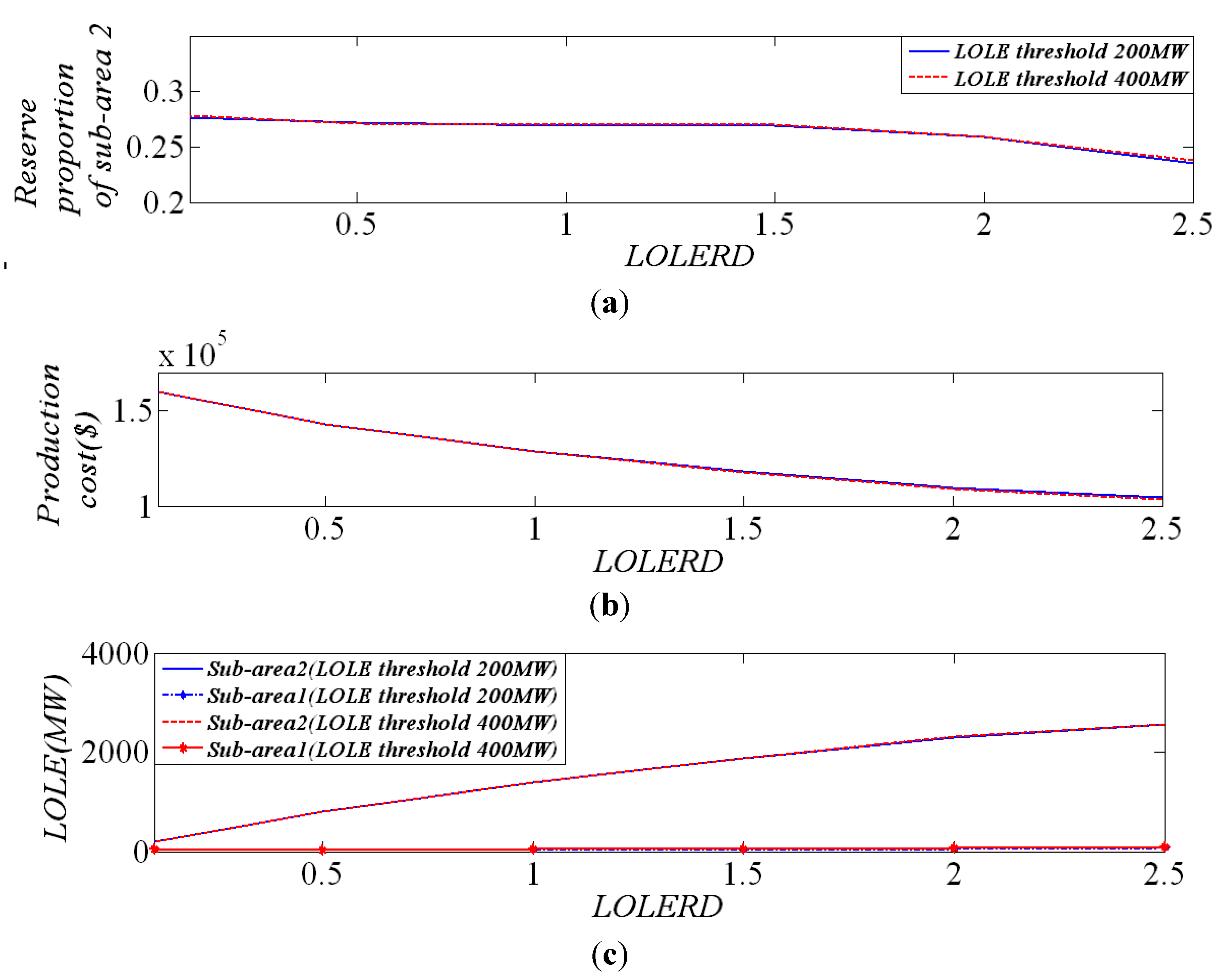
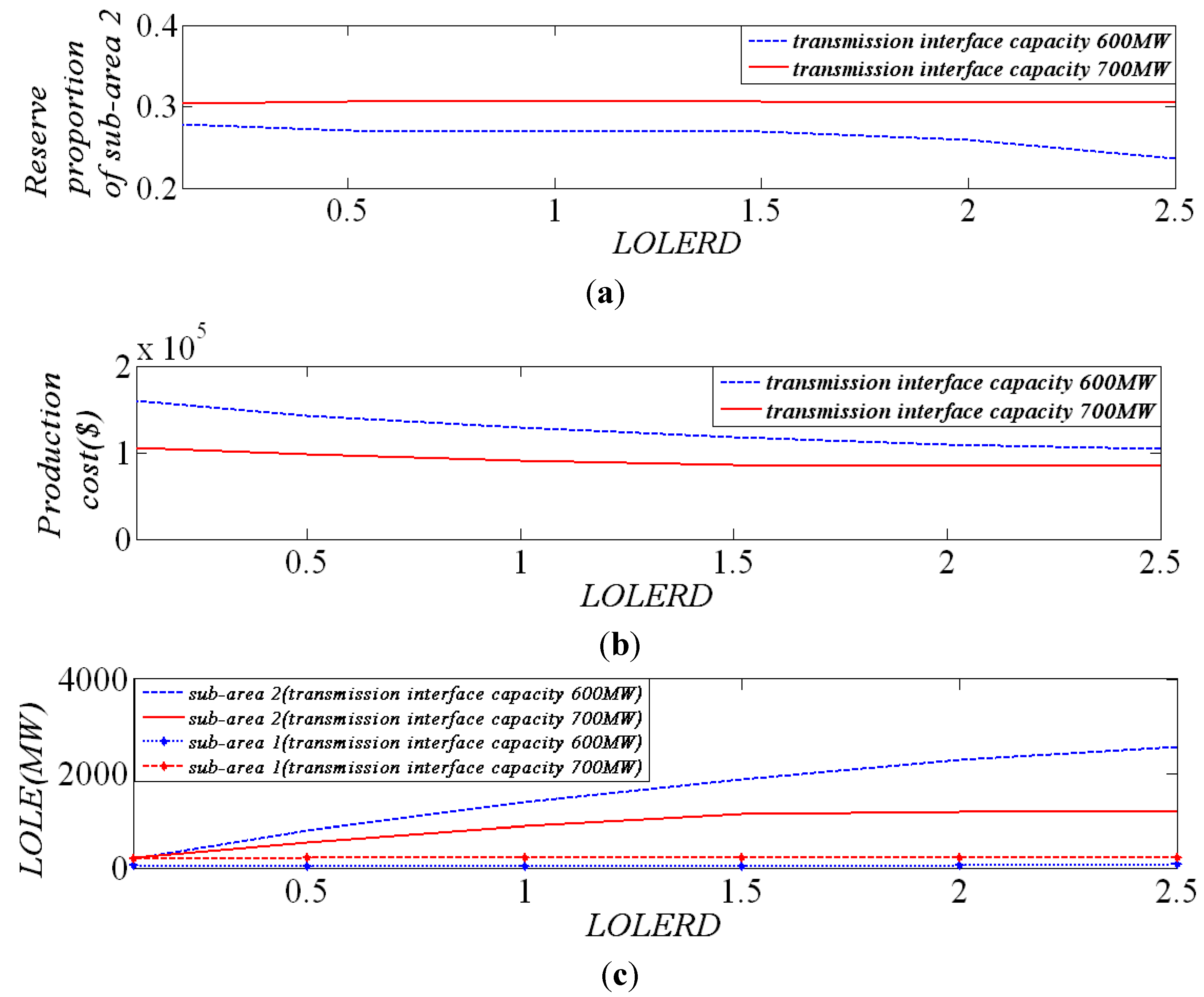
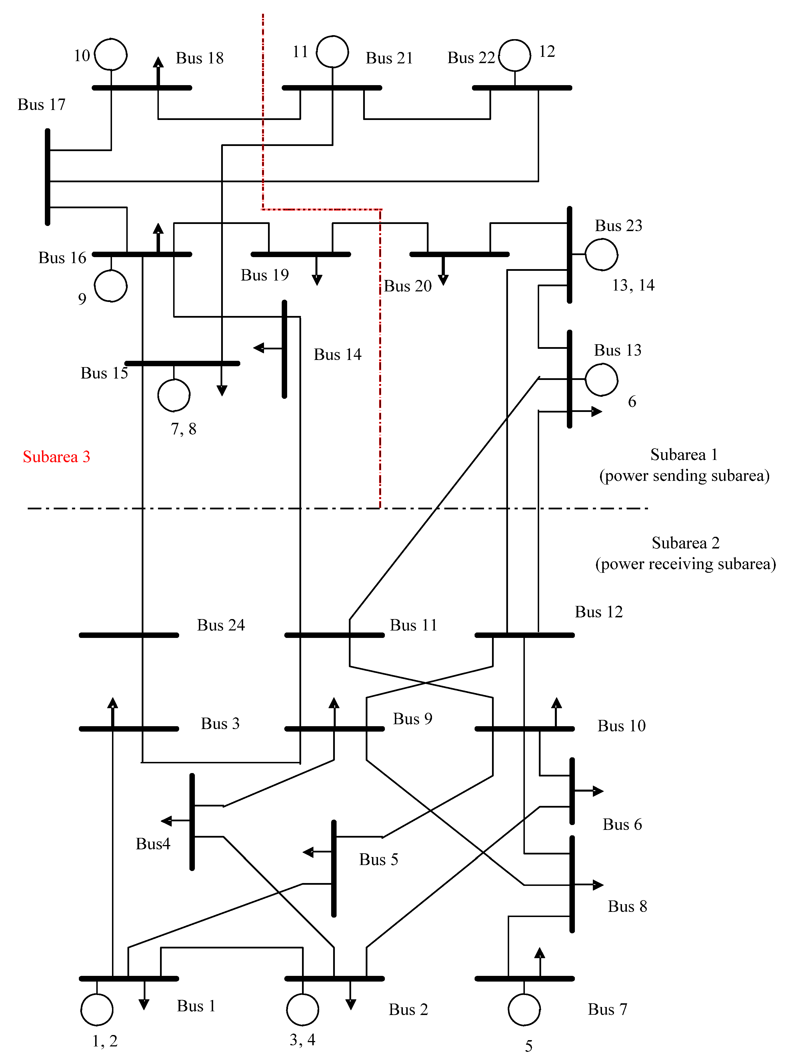
6.2. Fuzzy-Optimization-Based Multi-Sub-Area Reserve Allocation

The test system is divided into two sub-areas with the dark dashed line, as shown in Figure A1 in this part, in which the unit capacity of sub-area 2 takes up about 20% of the total generation capacity, while the load demand took about 47% of the total load demand. Hence, it is a power receiving subarea with the transmission interface between the two sub-areas heavy-loaded. The LOLE threshold is set to 250 MW, and the transmission interface limit is set to 600 MW.
(1) Effect of the preference factor
Three cases with k 2 = 0. 5 , k 3 = 0. 5 , k 2 = 0. 5 , k 3 = 0. 5 and k 2 = k 3 = 0 are respectively considered in this part, in which the upper limit of production cost is set to f 2 , m ax = 2 f 2 , min . The production cost with different operational risk indexes f 3 , max is shown in Figure 6.
It can be seen that when the optimistic attitude towards system reliability is taken, i.e., k2 takes a positive value and k3 takes negative value, the production cost is the lowest. When a pessimistic attitude towards system reliability is taken, i.e., k2 takes negative value and k3 takes a positive value, the production cost is the highest. Particularly, the production cost is in the middle when a neutral attitude towards system reliability is taken (i.e., k2 = k3 = 0).
Figure 6. Production cost under different preference factor values.
Energies 06 05357 g006
(2) Effect of LOLERD
Keeping the LOLE threshold and the transmission interface limit constant, the production cost and LOLE under different LOLERD values are given in Figure 7 in which the linear membership function is adopted. It can be seen from Figure 7 that when LOLERD decreases, the production cost increases while LOLE for the power receiving sub-area 2 decreases and the power sending sub-area 1 remains relatively constant. They gradually become consistent, indicating the validity of the proposed method on balancing the sub-area operational risk.
Figure 7. Effect of LOLERD on the production cost and LOLE.
Energies 06 05357 g007
(3) Effect of the LOLE threshold
Keeping all the other variables constant, the reserve allocation results of sub-area 2, the production cost and LOLE with different LOLERD are respectively shown in Figure 8, in which the LOLE threshold for the system is set respectively to 200 MW and 400 MW.
Figure 8. Results with different LOLE threshold. (a) Reserve allocation results of sub-area 2; (b) Production cost; (c) Relationship between subarea LOLE and LOLERD.
Energies 06 05357 g008
It can be seen that the curves are almost identical when the threshold of LOLE are respectively 200 MW and 400 MW, indicating a small sensitivity of LOLE threshold to the results under the same LOLERD value when the transmission interface is heavy-load. At the same time, a high sensitivity of LOLERD to the results is observed as there is an evident variation of the results with different LOLERD.
(4) Effect of the transmission interface capacity
The relationships between the reserve demand of sub-area 2, the production cost, LOLE and LOLERD are shown in Figure 9.
As can be seen, when the transmission interface capacity increases, the production cost decreases and the reserve demand of power receiving sub-area 2 increases. Meantime, the LOLE of sub-area 2 is remarkably reduced with only a small change of the power flow. The results indicate a high sensitivity of transmission interface capacity to both the economy and security, which also means that some measurements should be taken to reinforce the interconnection.
Figure 9. Results with different transmission interface limits. (a) Relationship between reserve proportion of sub-area 2 and LOLERD; (b) Relationship between the production cost and LOLERD; (c) Relationship between sub-area LOLE and LOLERD.
Energies 06 05357 g009
(5) Reserve allocation results
When f 3 , max takes the value of 0.5 and the other variables remain constant, the comparison of unit output and reserve capacity results of sub-area 2 between the proposed method and conventional probabilistic method during the 13th time period are respectively shown in Figure 10 and Figure 11.
Figure 10. Active power output of the units in sub-area 2.
Energies 06 05357 g010
Figure 11. Spinning reserve capacity of the units in sub-area 2.
Energies 06 05357 g011
It can be seen that when the proposed reserve balance factor is accounted for, the active power output of unit #5, which has a larger capacity and has reached its upper limit, is curtailed. The outputs of units #1 and #3, which have relatively smaller capacities, are increased. Thus, the reserve capacity of sub-area 2 is increased and the operational risk is correspondingly decreased. Overall, more reserve is allocated for the power receiving sub-area to cope with the wind power fluctuation or the generator outage when the transmission interface is heavy-load.
The proposed model has a heavier computational burden than a conventional economic dispatch problem, because of the nonlinear and non-convex constraints in the model. A Matlab program is developed for the proposed method, and tested on an Intel(R) Core(TM) 2 Duo CPU computer with 2 GB RAM. The average CPU time on IEEE RTS system is about 356.1 s, but its performance heavily depends on the initial values of the particle swarms. For the well-generated initial values, its computation time can be reduced to 56 s. However, in the worst cases, the calculation time is 756.07 s. As shown in Figure 12, we believe that there are still lots of works to do for improving the performance of the solution in the future.
Figure 12. Calculation time of the PSO method.
Energies 06 05357 g012
Meanwhile, as the main focus of this paper is to evaluate the effects of wind power generation on the allocation of spinning reserve for a multi-subarea power system, where the results can further be summarized to develop expert knowledge for real-time spinning reserve determination. And some optimization techniques like the successive-linearization technique can be investigated if a fast speed is required in the future work.
(6) Reserve allocation results on a three-subarea test system
In this part, the IEEE RTS test system is further divided into a three sub-area system with the red dashed line, as shown in Figure A1. The load demand of sub-area 3 took about 13.3% of the total load demand, and the capacity of the transmission interface was set to be 100 MW. The reserve allocation results comparison of the reserve capacity between the proposed method and conventional probabilistic method during the 14th time period with f3,max = 0.5 is shown in Figure 13.
Figure 13. Spinning reserve capacities of all the units in the system.
Energies 06 05357 g013
It can be seen from Figure 13 that when the proposed reserve balance is considered, the reserve capacity of unit #10 which has the largest installed capacity in sub-area 3 is reduced. The reserve capacity of unit #11, which is the largest thermal unit in sub-area 1, is increased. Meanwhile, the reserve capacity in sub-area 2 keeps constant. Accordingly, the reserve capacity of sub-area 1, which has large-scale wind power integration, is increased and the operational risk is correspondingly decreased.

7. Conclusions

Due to the large-scale penetration of wind power and its high fluctuation characteristics, the power flow of the grid varies intensively and drastically, which often makes the transmission interface margin insufficient and results in problems of local reserve inadequacy. Thus, the spinning reserve allocation problem for multi-area system becomes especially prominent for operational security of wind power systems. And it is investigated in this paper. Firstly, a risk-based multi-objective spinning reserve allocation optimization model is proposed. The relationship between the loss of load expectation and spinning reserve taken large-scale wind power integration into account is derived. Then, a fuzzy optimization method is applied to transform the multi-objective optimization problem into a single-objective optimization one. Finally, a particle swarm optimization method is applied to solve it.
From the numerical tests on IEEE RTS system, it can be seen that when the proposed reserve allocation method is considered, more reserve capacity will be reserved for the sub-areas with large-scale wind power integration or high load shedding losses when the transmission interface is heavy-load. With more reserve capacity, the scenarios of local reserve inadequacy or transmission interface overload due to the variation of wind power or forced outage of conventional units can be handled well. In this procedure, the unit output is reallocated compared with the results of the conventional method, and the reserve of those generators with relatively large capacities decreases while those with relatively small capacities increases. Overall, the sub-area operational risk is balanced by the reserve allocation method, and the effectiveness of the proposed method is validated.

Acknowledgments

This work is supported by National High Technology Research Program (2011AA05A101), National Science Foundation of China (51177080, 51190105) and New Century Excellent University Talents (NCET-11-0281).

Conflicts of Interest

The authors declare no conflict of interest.

Nomenclature

Sets
G w i n d Set of wind farms.
G Set of conventional units.
Parameters
D j t Predicted load demand of area j during time period t.
D t Predicted load demand of the whole system during time period t.
nNumber of control sub-areas.
p j t f    Predicted wind power output of wind farm j during time period t.
p j t max Predicted maximum available output of wind farm j during time period t.
λ j Penalty coefficient for wind power curtailment.
a i / b i / c i Production cost coefficients of thermal unit i.
N Number of thermal units.
t 0 / T Initial and last time period of the optimization.
E t h r e s h Threshold of LOLE.
p ¯ i / p _ i Maximum/minimum generation output of unit i.
Δ p d i / Δ p u i Downward/upward ramp rate of unit i.
T 15 15-min time duration.
T 10 Time duration, usually 10 min, for the calculation of unit spinning reserve contribution [1,2].
LNumber of the transmission interfaces.
k l i Generation distribution shift factor of unit i to transmission interface l.
T L l ¯ / T L l _ Positive/negative power flow limit of transmission interface l with bus loads excluded.
λ / μ The failure rate and the repair rate of a unit.
HThe swarm size.
γ i / ζ j Penalty coefficient for equality/inequality constraints of the PSO optimization.
ωmax/ωminMaximum/minimum inertia weight.
k Iteration number.
k max The maximum iteration number.
c1/c2Acceleration constants.
p f    Total predicted wind power output results.
Variables
E t       LOLE of the whole system during time period t.
E 1 t / E 2 t / E 3 t LOLE with no/one/two generator outage(s) accounted during time period t.
E t M / E t N LOLE of sub-area M/N during time period t.
I t Loss of load expectation ratio deviation (LOLERD).
T L l t Power flow of transmission interface l during time period t, which can be calculated from the output of generators and loads multiplied with their corresponding sensitivity.
E G j t LOLE of area j during time period t.
r j t LOLE ratio (LOLER) of area j during time period t.
r ¯ t The average of LOLER of all the control sub-areas.
p j t w Wind power generation schedule of wind farm j during time period t.
p i t Generation schedule of conventional thermal unit i during time period t.
f 1 Penalty term for wind power curtailment.
f 2 Production cost of conventional thermal units.
f 3 Operating risk index of the system.
R t u / R t d Up/down spinning reserve of the system during time period t.
R i t u / R i t d Upward/downward spinning reserve contribution of unit i during time period t.
α 1 / β 1 / γ 1 α 2 / β 2 / γ 2 
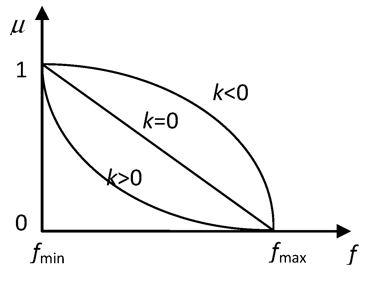
Coefficients of the membership functions.
f i , max / f i , min Upper/lower limits of the production cost or operational risk index for conventional units.
k i The preference factor ( k2 is the cost preference factor and k3 is the risk preference factor).
xPredicted error of wind power and load demand.
F O R i , t The forced outage rate of unit i during time period t.
f ( x ) 
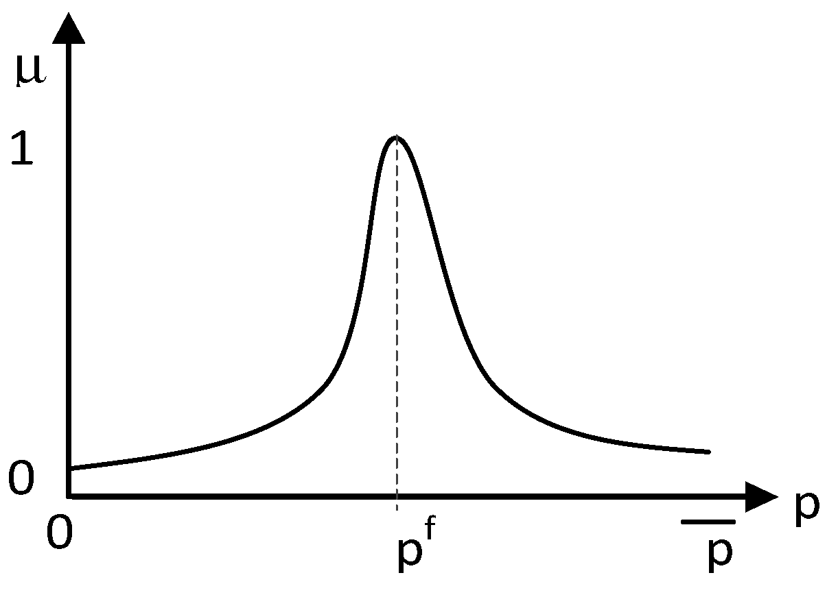
Probability density function of the forecast error.
σ t Standard deviation of the forecast error.
R t M N Inter-zonal supply of the reserve.
R t M / R t N Spinning reserve of sub-area M /sub-area N during time period t.
x i j t Position of unit j of particle i during time period t.
v i j t Velocity of unit j of particle i during time period t.
P ¯ i , t / P _ i , t Upper/lower limits of unit i with ramp rate constraints accounted.
xi(k)Position of particle i during iteration k.
ω The inertia weight.
μ 1 / μ 2 / μ 3 Membership function of wind curtailment/economics/security

Appendix

Table A1. Unit parameters of the IEEE RTS system.
Unit No. p ¯ i piaibici
14000.0176130800
2152300.007143.66424.62
34000.0176130800
4152300.007143.66424.62
530075016.082344.56
65912070.002448.582498.27
760120.065756.56431.93
8155540.008312.39382.24
9155540.008312.39382.24
104001000.000214.42395.37
114001000.000214.42395.37
1230060016.082344.56
133101080.004212.39764.48
147000000
Figure A1. IEEE RTS system with two/three sub-area division.
Energies 06 05357 g014

References

  1. Xia, L.M.; Gooi, H.B.; Bai, J. Probabilistic Spinning Reserves with Interruptible Loads. In Proceedings of IEEE Power & Engineering Society General Meeting, Piscataway, NJ, USA, 6–10 June 2004.
  2. Venkatesh, B.; Peng, Yu; Gooi, H.B.; Choling, D. Fuzzy MILP unit commitment incorporating wind generators. IEEE Trans. Power Syst. 2008, 23, 1738–1746. [Google Scholar]
  3. Ummels, B.C.; Gibescu, M.; Pelgrum, E.; Kling, W.L.; Brand, A.J. Impacts of wind power on thermal generation unit commitment and dispatch. IEEE Trans. Energy Convers. 2007, 22, 44–51. [Google Scholar]
  4. Soder, L. Reserve margin planning in a wind-hydro-thermal power systems. IEEE Trans. Power Syst. 1993, 8, 564–571. [Google Scholar] [CrossRef]
  5. Ela, E.; Kirby, B.; Lannoye, E.; Milligan, M.; Flynn, D.; Zavadil, B.; O’Malley, M. Evolution of Operating Reserve Determination in Wind Power Integration Studies. In Proceedings of the IEEE Power & Energy Society General Meeting, Minneapolis, MN, USA, 25–29 July 2010.
  6. Wu, W.C.; Zhang, B.M.; Chen, J.H.; Zhen, T.Y. Multiple Time-Scale Coordinated Power Control System to Accommodate Significant Wind Power Penetration and Its Real Application. In Proceedings of the 2012 IEEE Power & Energy Society General Meeting, San Diego, CA, USA, 22–26 July 2012.
  7. Zhang, G.Q.; Wu, W.C.; Zhang, B.M. Optimization of operation reserve coordination considering wind power integration. Autom. Electr. Power Syst. 2011, 35, 15–19. [Google Scholar]
  8. Lee, T.-Y. Optimal spinning reserve for a wind-thermal power system using EIPSO. IEEE Trans. Power Syst. 2007, 22, 1612–1621. [Google Scholar] [CrossRef]
  9. Ortega-Vazquez, M.A.; Kirchen, D.S. Should the Spinning Reserve Procurement in Systems with Wind Power Generation Be Deterministic or Probabilistic. In Proceedings of the 1st International Conference on Sustainable Power Generation and Supply (SUPERGEN), Nanjing, China, 6–7 April 2009; pp. 1–9.
  10. Doherty, R.; O’Malley, M. A new approach to quantify reserve demand in systems with significant installed wind capacity. IEEE Trans. Power Syst. 2005, 20, 587–595. [Google Scholar] [CrossRef]
  11. Zhou, W.; Peng, Y.; Sun, H. Optimal wind-thermal coordination dispatch based on risk reserve constraints. Eur. Trans. Electr. Power 2011, 21, 740–756. [Google Scholar] [CrossRef]
  12. Hetzer, J.; Yu, D.C.; Bhattarai, K. An economic dispatch model incorporating wind power. IEEE Trans. Energy Convers. 2008, 23, 603–611. [Google Scholar] [CrossRef]
  13. Morales, J.M.; Conejo, A.J.; Perez-Ruiz, J. Economic valuation of reserves in power systems with high penetration of wind power. IEEE Trans. Power Syst. 2009, 24, 900–910. [Google Scholar] [CrossRef]
  14. Streiffert, D. Multi-area economic dispatch with tie line constraints. IEEE Trans. Power Syst. 1995, 10, 1946–1951. [Google Scholar] [CrossRef]
  15. Ma, X.W.; Sun, D.; Cheung, K. Energy and reserve dispatch in a multi-zone electricity market. IEEE Trans. Power Syst. 1999, 14, 913–919. [Google Scholar] [CrossRef]
  16. Liang, M.; Lee, S.T.; Zhang, P.; Rose, V.; Cole, J. Short-Term Probabilistic Transmission Congestion Forecasting. In Proceedings of the Third International Conference on Electric Utility Deregulation and Restructuring and Power Technologies (DRPT), Nanjing, China, 6–9 April 2008; pp. 764–770.
  17. Chen, C.-L.; Lee, T.-Y. Impact Analysis of Transmission Capacity Constraints on Wind Power Penetration and Production Cost in Generation Dispatch. In Proceedings of the International Conference on Intelligent Systems Applications to Power Systems(ISAP), Toki Messe, Niigata, Japan, 5–8 November 2007; pp. 1–6.
  18. Bjorgan, R.; Liu, C.-C.; Lawarree, J. Financial risk management in a competitive electricity market. IEEE Trans. Power Syst. 1999, 14, 1285–1291. [Google Scholar] [CrossRef]
  19. Liu, Y.; Guan, X. Purchase allocation and demand bidding in electric power markets. IEEE Trans. Power Syst. 2003, 18, 106–112. [Google Scholar] [CrossRef]
  20. Conejo, A.J.; Nogales, F.J.; Arroyo, J.M.; Garcia-Bertrand, R. Risk-constrained self-scheduling of a thermal power producer. IEEE Trans. Power Syst. 2004, 19, 1569–1574. [Google Scholar] [CrossRef]
  21. Doherty, R.; O’Malley, M. Quantifying Reserve Demands due to Increasing Wind Power Penetration. In Proceedings of IEEE Bologna Power Technology Conference, Bologna, Italy, 23–26 June 2003.
  22. Lei, Y.; Han, X.; Yu, D. Multi-Time Scale Decision-Making Method of Synergistic Dispatch. In Proceedings of the 2012 IEEE Innovative Smart Grid Technologies—Asia, Tianjin, China, 21–24 May 2012.
  23. Cheung, K.; Wang, X.; Chiu, B.-C.; Xiao, Y.; Rios-Zalapa, R. Generation Dispatch in a Smart Grid Environment. In Proceedings of the 2010 Innovative Smart Grid Technologies, Gaithersburg, MD, USA, 19–21 January 2010.
  24. Liang, R.H.; Liao, J.H. A fuzzy-optimization approach for generation scheduling with wind and solar energy systems. IEEE Trans. Power Syst. 2007, 22, 1665–1674. [Google Scholar]
  25. Venkatesh, B.; Sadasivam, G.; Khan, M.A. A new optimal reactive power scheduling method for loss minimization and voltage stability margin maximization using successive multi-objective fuzzy LP technique. IEEE Trans. Power Syst. 2000, 15, 844–851. [Google Scholar] [CrossRef]
  26. Amjady, N.; Aghaei, J.; Shayanfar, H.A. Stochastic multiobjective market clearing of joint energy and reserves auctions ensuring power system security. IEEE Trans. Power Syst. 2009, 24, 1841–1854. [Google Scholar] [CrossRef]
  27. Fabbri, A.; Román, T.G.S.; Abbad, J.R.; Quezada, V.H.M. Assessment of the cost associated with wind generation prediction errors in a liberalized electricity market. IEEE Trans. Power Syst. 2005, 20, 1440–1446. [Google Scholar] [CrossRef]
  28. Billinton, R.; Ghajar, R. Evaluation of the marginal outage costs of generating systems for the purposes of spot pricing. IEEE Trans. Power Syst. 1994, 9, 68–75. [Google Scholar] [CrossRef]
  29. Liu, H.; Sun, Y.; Cheng, L.; Wang, P.; Xiao, F. Online short-term reliability evaluation using a fast sorting technique. IET Gener. Transm. Distrib. 2008, 2, 139–148. [Google Scholar] [CrossRef]
  30. Kennedy, J.; Eberhart, R. Particle Swarm Optimization. In Proceedings of the International Conference on Neural Networks, Perth, Australia, 27 November–1 December 1995; pp. 1942–1948.
  31. Kennedy, J.; Eberhart, R. Swarm Intelligence; Morgan Kaufmann Publishers: San Francisco, CA, USA, 2001. [Google Scholar]
  32. Angeline, P.J. Evolutionary Optimization versus Particle Swarm Optimization: Philosophy and Performance Differences. In Proceedings of the 7th International Conference on Evolutionary Programming, San Diego, CA, USA, 25–27 March 1998.
  33. Hassan, R.; Cohanim, B.; Weck, O. A Comparison of Particle Swarm Optimization and the Genetic Algorithm. In Proceedings of the 46th AIAA/ASME/ASCE/AHS/ASC Structures, Structural Dynamics & Materials Conference, Austin, TX, USA, 18–21 April 2005.
  34. Elbeltagi, E.; Hegazy, T.; Grierson, D. Comparison among five evolutionary-based optimization algorithms. Adv. Eng. Inform. 2005, 19, 43–53. [Google Scholar] [CrossRef]
  35. Gaing, Z.L. Constrained Optimal Power Flow by Mixed-Integer Particle Swarm Optimization. In Proceedings of the IEEE Power Engineering Society General Meeting, San Francisco, CA, USA, 12–16 June 2005; pp. 243–250.
  36. Selvakumar, A.I.; Thanushkodi, K. A new particle swarm optimization solution to nonconvex economic dispatch problems. IEEE Trans. Power Syst. 2007, 22, 42–51. [Google Scholar]
  37. Gaing, Z.L. Constrained Dynamic Economic Dispatch Solution Using Particle Swarm Optimization. In Proceedings of IEEE Power & Engineering Society General Meeting, Piscataway, NJ, USA, 6–10 June 2004.
  38. Gaing, Z.L. Particle swarm optimization to solving the economic dispatch considering the generator constraints. IEEE Trans. Power Syst. 2003, 18, 1187–1195. [Google Scholar] [CrossRef]
  39. Coath, G.; Al-Dabbagh, M.; Halgamuge, S. Particle swarm optimization for reactive power and voltage control with grid-integrated wind farms. In Proceedings of IEEE Power & Engineering Society General Meeting, Piscataway, NJ, USA, 6–10 June, 2004.

