Probabilistic Approach to Optimizing Active and Reactive Power Flow in Wind Farms Considering Wake Effects


Abstract
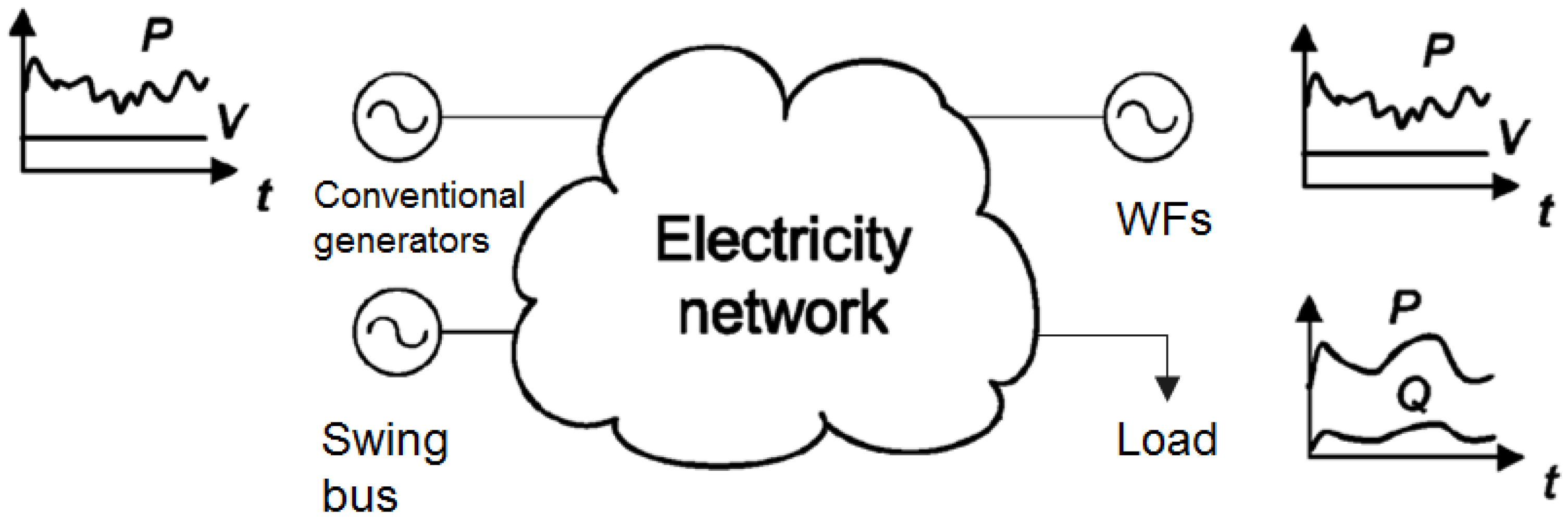
:1. Introduction
- ➢
- uncertainty modeling of load and wind speed
- ➢
- correlated wind speed and wake effect
- ➢
- PV bus model for wind turbines and alternating current (AC) network constraints
- ➢
- time series power flow analysis
2. Wind Speed and Load Modeling

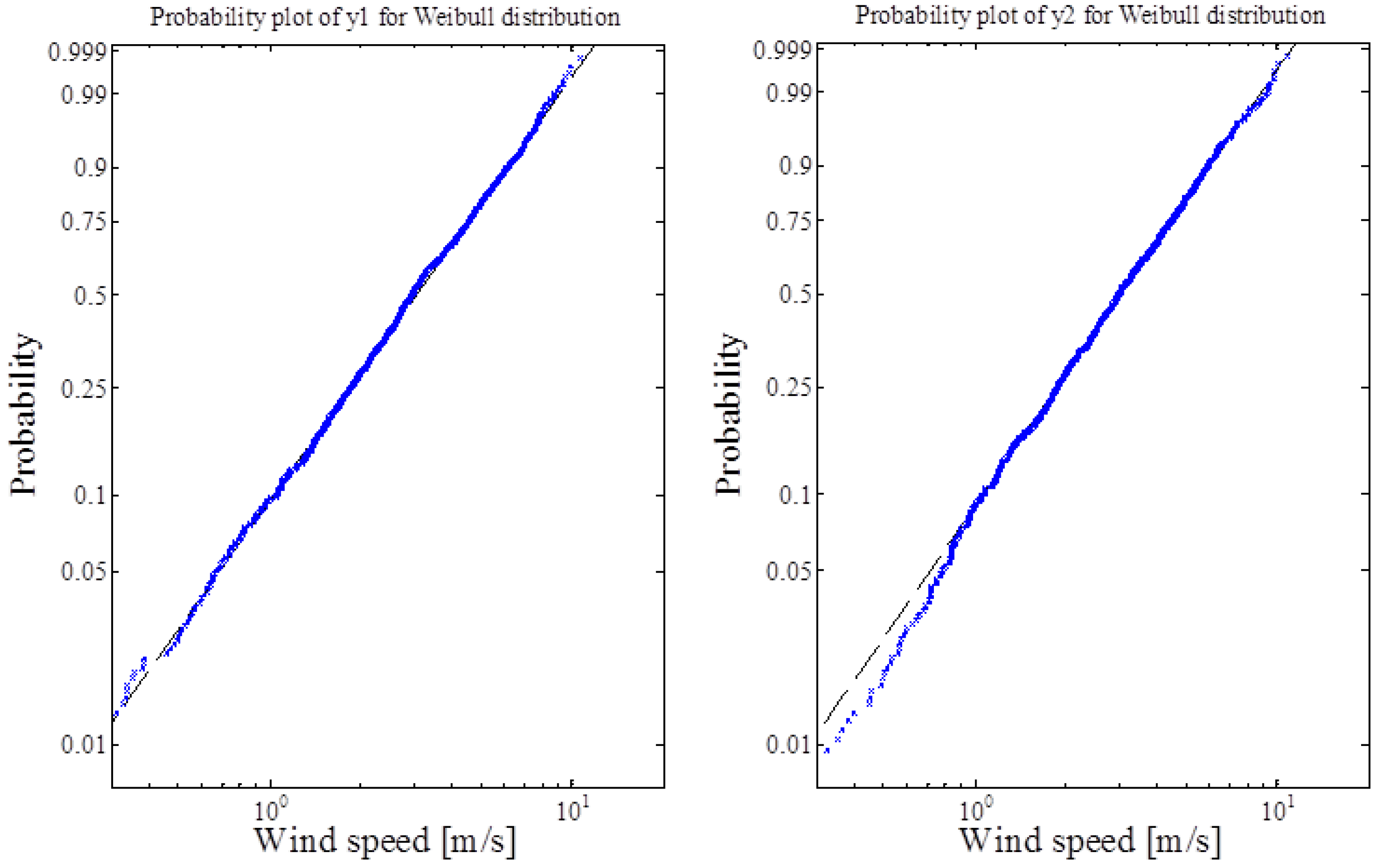
2.1. Wind Speed
2.2. Wind Speed Correlation
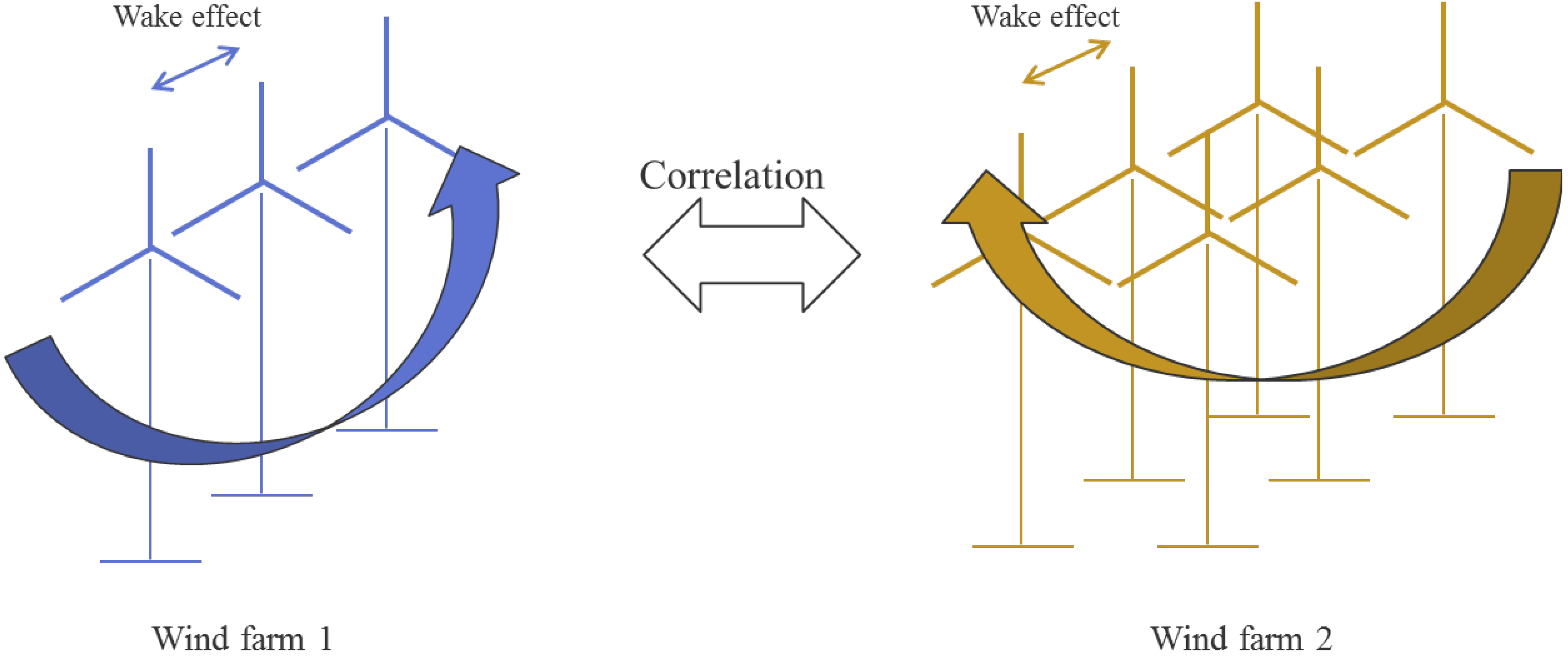
2.3. Wake Effect
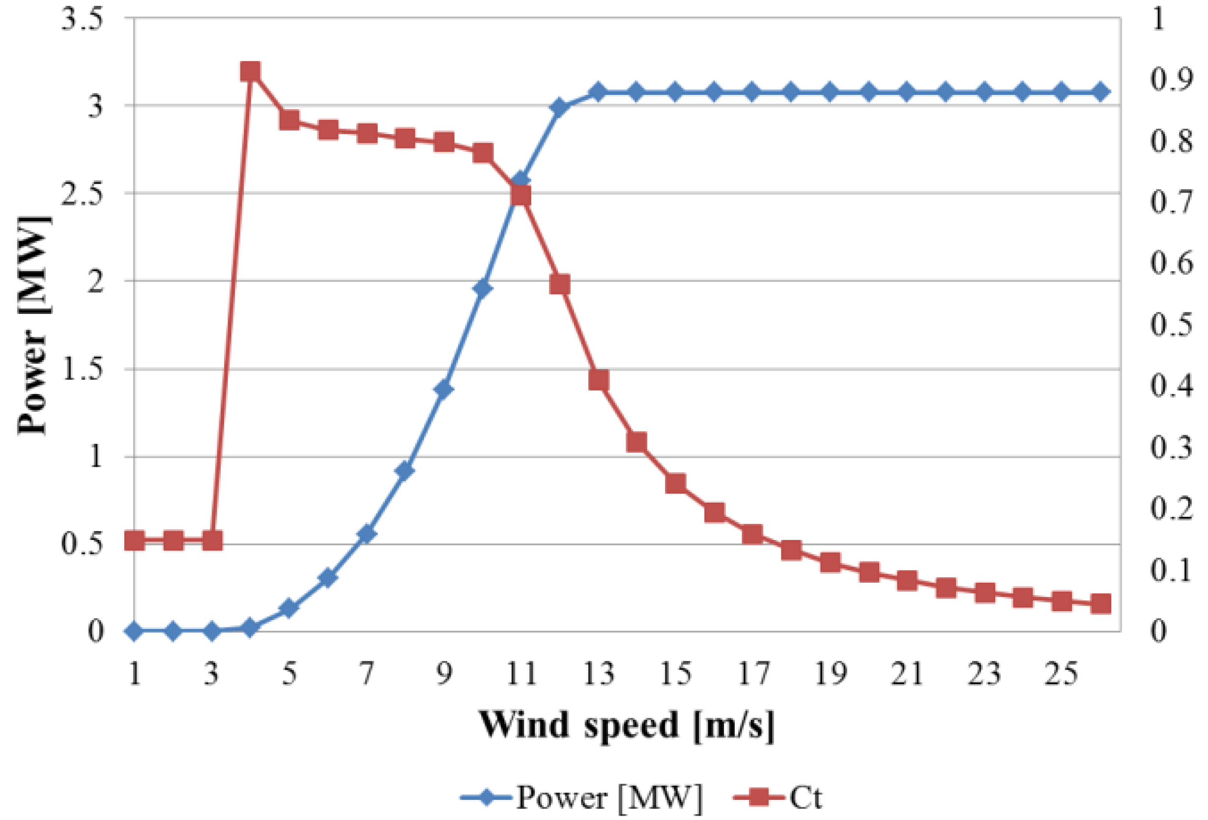
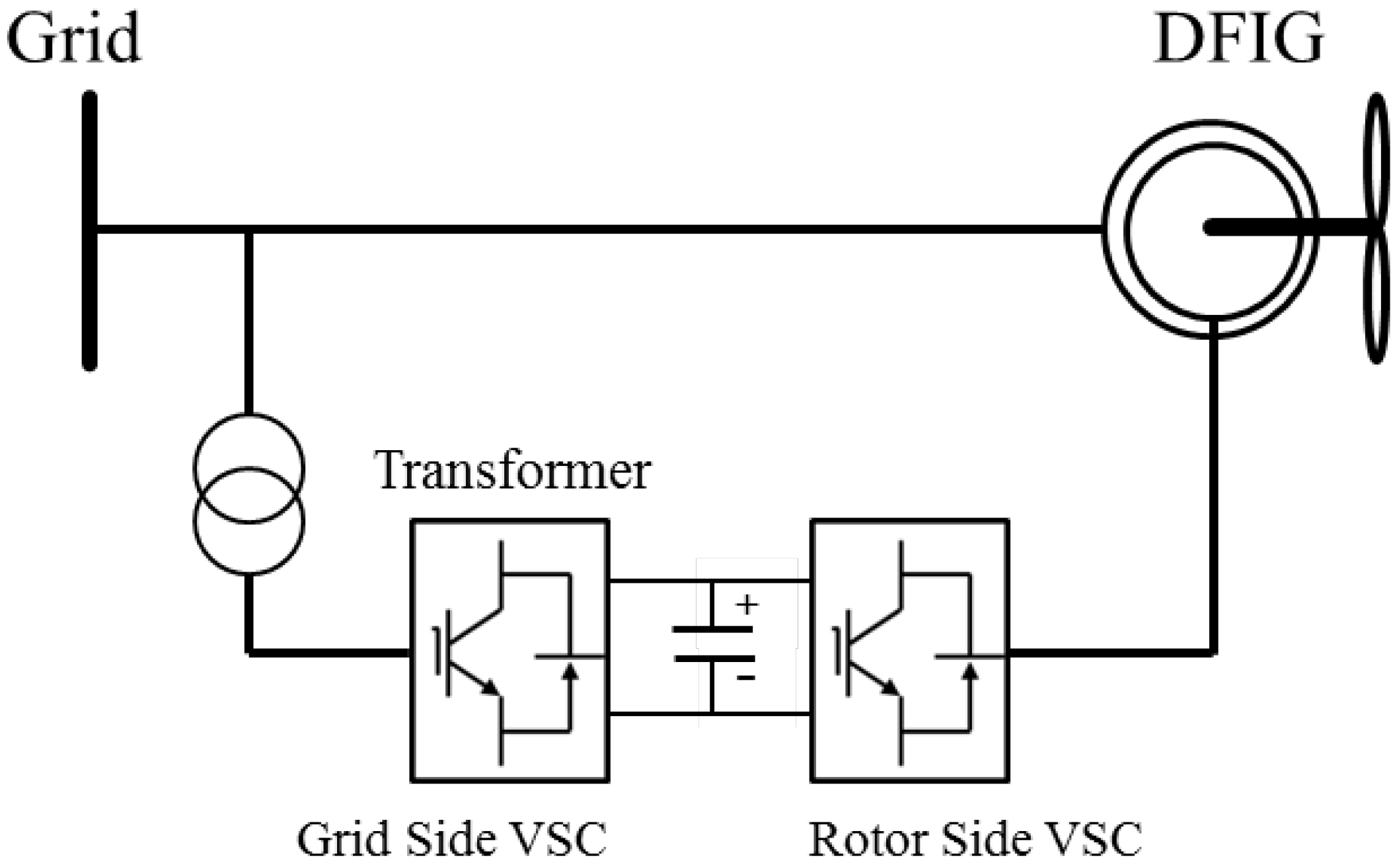
3. Wind Turbine Modeling Considering Power Factor Control

4. Problem Formulation
4.1. Probabilistic Optimal Power Flow
- power flow equations:
- power output limit of thermal generating units:
- bus voltage limit:
- power flow limits of line from bus i to bus j:
4.2. Primal-Dual Interior Point Method


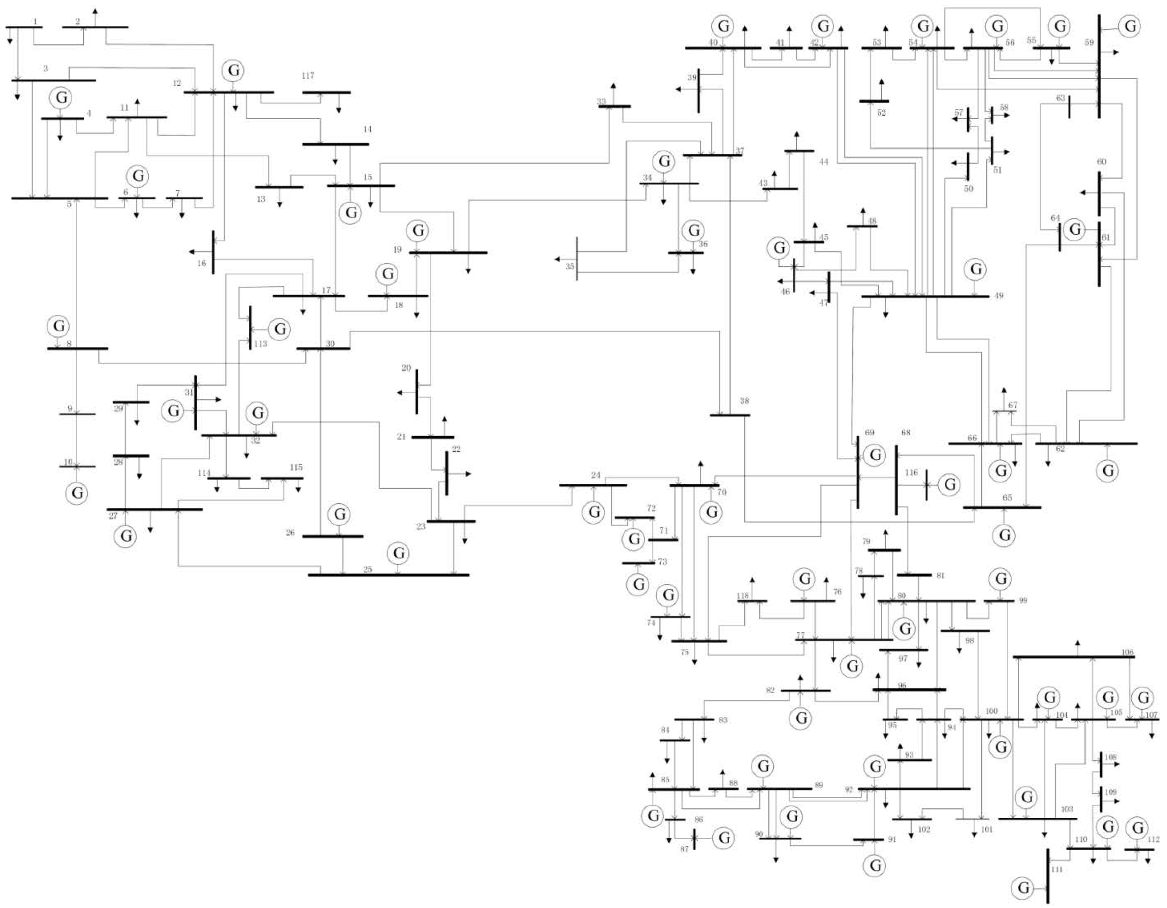
5. Numerical Results

| Unit (MW) | α (lb/h) | β (lb/MWh) | γ (lb/MW2h) | ζ (lb/h) | λ (1/MW) |
|---|---|---|---|---|---|
| <30 | 6.131 | 5.555 | 5.151 | 1 | 6.667 |
| 31–50 | 4.258 | 5.094 | 4.586 | 1 | 8.000 |
| 51–100 | 5.326 | 3.550 | 3.380 | 2 | 2.000 |
| 101–200 | 4.258 | 5.094 | 4.586 | 1 | 8.000 |
| 201–300 | 2.543 | 6.047 | 5.638 | 5 | 3.333 |
| >300 | 4.091 | 5.554 | 6.490 | 2 | 2.857 |
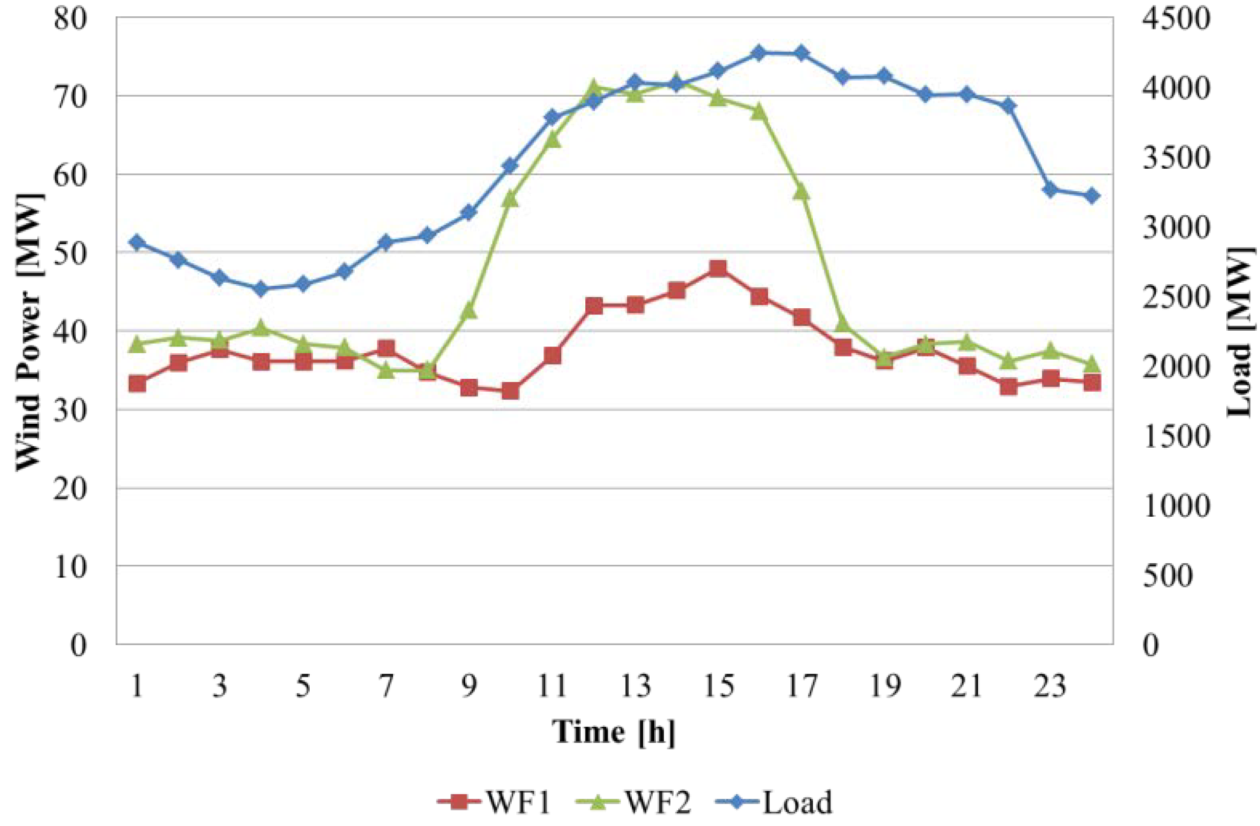
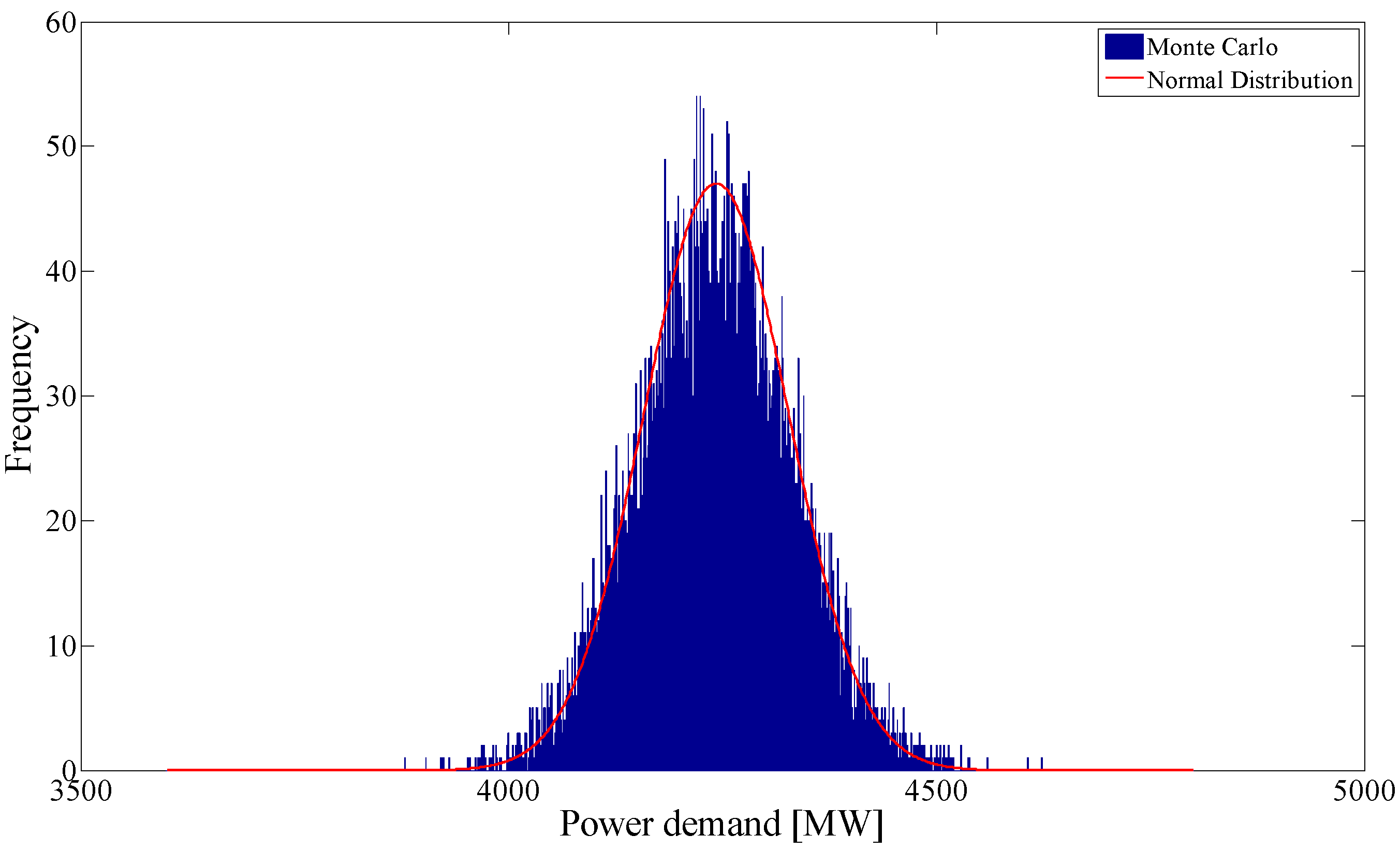
5.1. Load and Wind Power Uncertainties


| Title | WF1 | WF2 |
|---|---|---|
| Mean value μ | 5.95 | 6.1 |
| Standard deviation σ | 3.35 | 3.16 |
| Scale parameter c | 6.7 | 6.8 |
| Shape parameter k | 1.83 | 1.93 |
| Correlation coefficient | ||

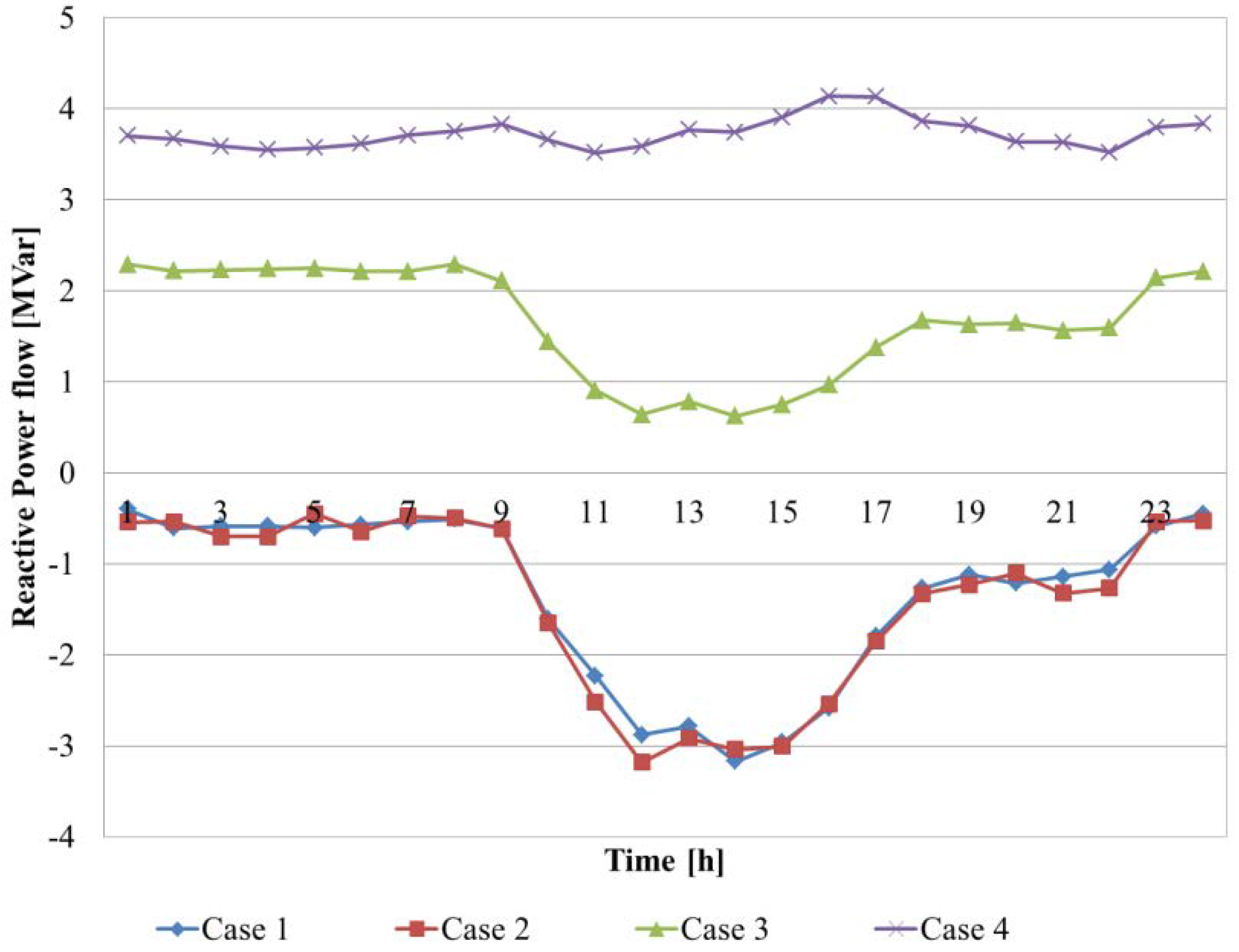
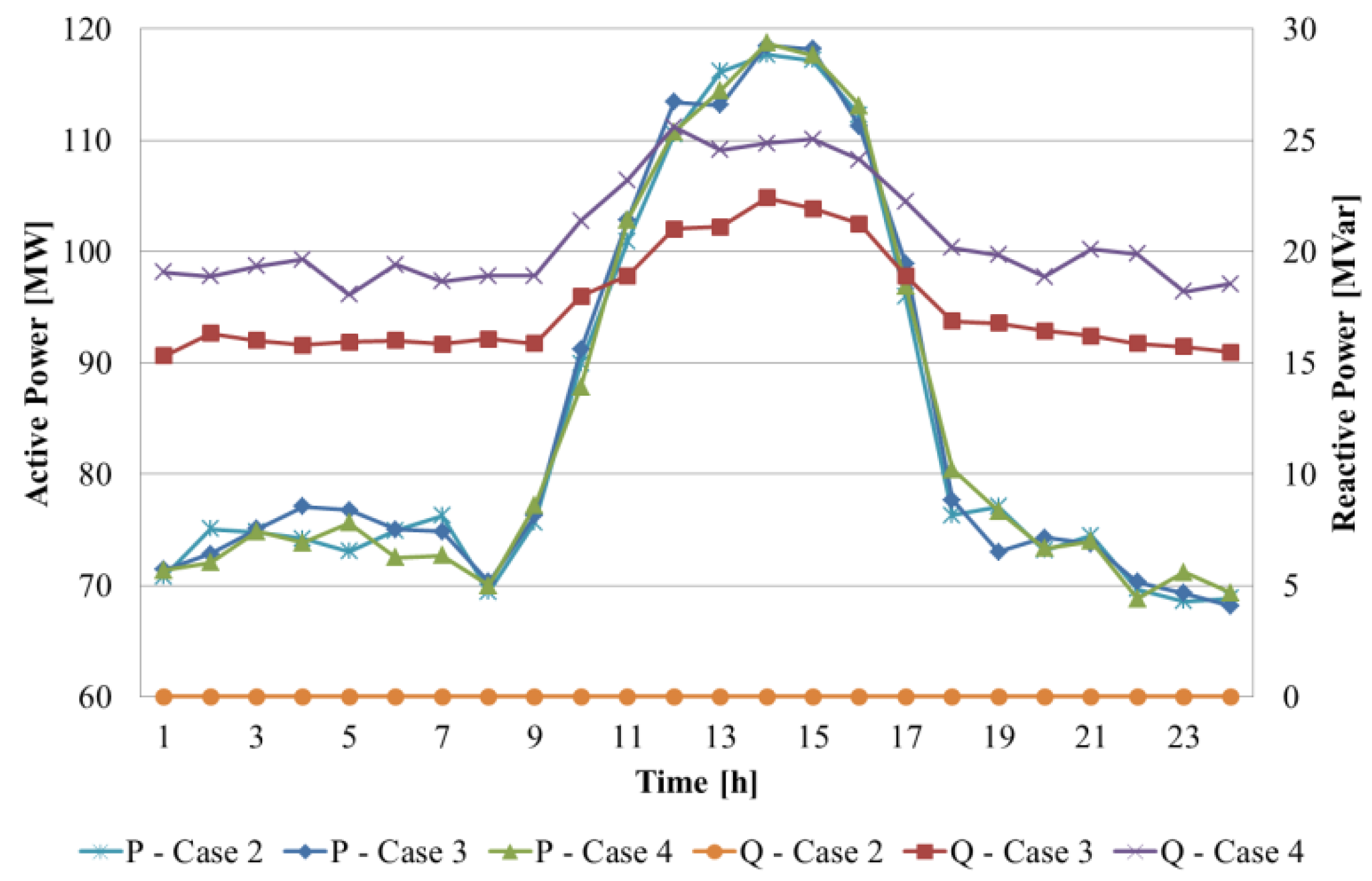
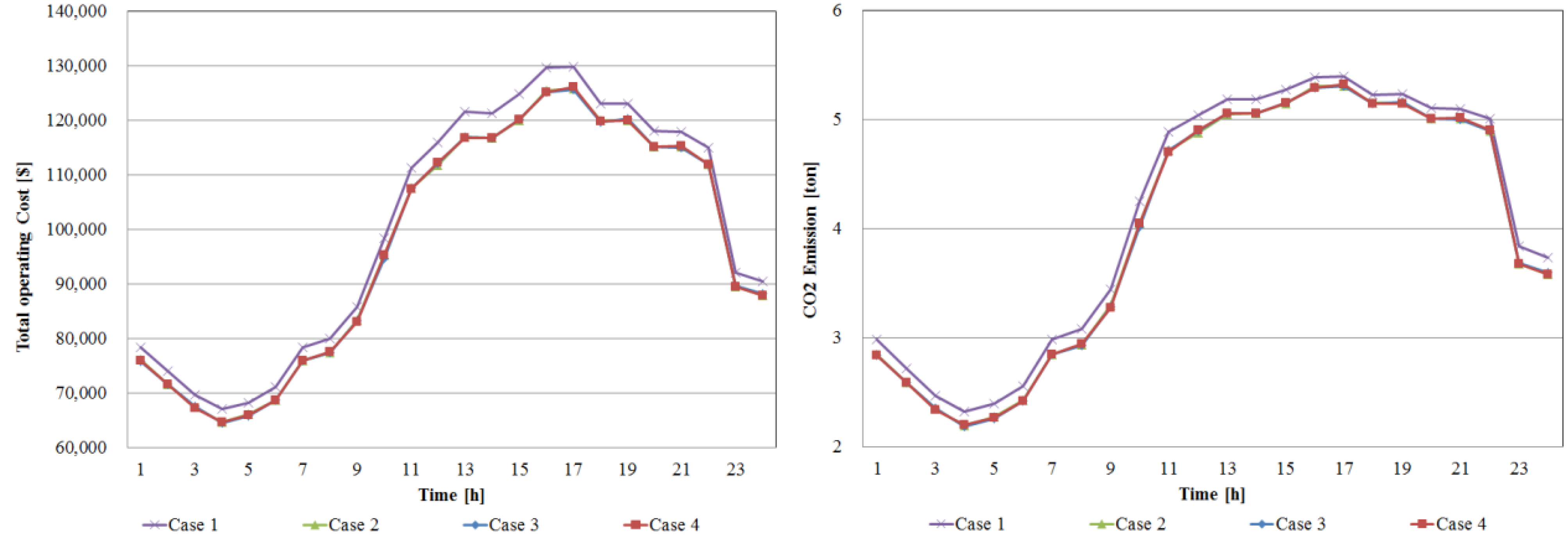
5.2. Probabilistic OPF Solutions
- Case 1: no wind power considered;
- Case 2: pf = 1;
- Case 3: pf = 0.95 lagging;
- Case 4: pf = 0.9 lagging.
| Case | Total operating cost ($) | P loss (MW) | CO2 emission (ton) | Wind power generation | ||
|---|---|---|---|---|---|---|
| P (MW) | Q (MVar) | CP (%) | ||||
| 1 | 2,405,677 | 1,568 | 99 | 0 | 0 | 0 |
| 2 | 2,331,241 | 1,552 | 96 | 2,033 | 0 | 28.2 |
| 3 | 2,330,318 | 1,550 | 96 | 2,043 | 420 | 28.3 |
| 4 | 2,331,065 | 1,545 | 96 | 2,036 | 498 | 28.2 |
| Case | Line | From bus | To bus | Time | Total | |||||||||||||||||||||||
|---|---|---|---|---|---|---|---|---|---|---|---|---|---|---|---|---|---|---|---|---|---|---|---|---|---|---|---|---|
| 1 | 2 | 3 | 4 | 5 | 6 | 7 | 8 | 9 | 10 | 11 | 12 | 13 | 14 | 15 | 16 | 17 | 18 | 19 | 20 | 21 | 22 | 23 | 24 | |||||
| 1 | 10 | 11 | 4 | −0.4 | −0.6 | −0.6 | −0.6 | −0.6 | −0.6 | −0.5 | −0.5 | −0.6 | −1.6 | −2.2 | −2.9 | −2.8 | −3.2 | −3.0 | −2.6 | −1.8 | −1.3 | −1.1 | −1.2 | −1.1 | −1.1 | −0.6 | −0.4 | 89 |
| 11 | 11 | 5 | −5.6 | −5.6 | −5.4 | −5.3 | −5.3 | −5.4 | −5.7 | −5.8 | −6.0 | −6.9 | −7.4 | −8.0 | −7.9 | −8.3 | −8.1 | −7.8 | −7.2 | −6.7 | −6.6 | −6.7 | −6.6 | −6.5 | −6.1 | −6.0 | ||
| 12 | 11 | 12 | 16.7 | 15.7 | 15.6 | 15.5 | 15.5 | 15.7 | 16.3 | 16.3 | 16.9 | 16.8 | 17.2 | 16.3 | 16.2 | 15.5 | 15.8 | 16.3 | 17.5 | 18.8 | 18.9 | 19.0 | 19.1 | 19.3 | 17.6 | 17.6 | ||
| 16 | 11 | 13 | −5.4 | −5.3 | −5.3 | −5.2 | −5.2 | −5.3 | −5.3 | −5.4 | −5.3 | −5.2 | −5.1 | −5.1 | −5.2 | −5.2 | −5.3 | −5.5 | −5.6 | −5.6 | −5.7 | −5.5 | −5.5 | −5.5 | −5.5 | −5.5 | ||
| 2 | 10 | 11 | 4 | −0.5 | −0.5 | −0.7 | −0.7 | −0.4 | −0.6 | −0.5 | −0.5 | −0.6 | −1.7 | −2.5 | −3.2 | −2.9 | −3.0 | −3.0 | −2.5 | −1.9 | −1.3 | −1.2 | −1.1 | −1.3 | −1.3 | −0.5 | −0.5 | 95 |
| 11 | 11 | 5 | −5.2 | −5.0 | −5.0 | −4.9 | −4.7 | −5.0 | −5.1 | −5.2 | −5.4 | −6.4 | −7.2 | −7.8 | −7.5 | −7.6 | −7.6 | −7.3 | −6.7 | −6.3 | −6.2 | −6.0 | −6.3 | −6.2 | −5.5 | −5.5 | ||
| 12 | 11 | 12 | 15.3 | 15.1 | 14.5 | 14.1 | 15.2 | 14.6 | 15.6 | 15.6 | 16.0 | 15.7 | 15.6 | 14.5 | 15.1 | 15.0 | 14.9 | 15.3 | 16.5 | 17.7 | 17.9 | 18.5 | 17.8 | 17.8 | 17.0 | 16.7 | ||
| 16 | 11 | 13 | −4.5 | −4.5 | −4.4 | −4.4 | −4.3 | −4.4 | −4.5 | −4.5 | −4.5 | −4.3 | −4.3 | −4.3 | −4.3 | −4.3 | −4.4 | −4.6 | −4.7 | −4.7 | −4.7 | −4.6 | −4.7 | −4.7 | −4.5 | −4.6 | ||
| 3 | 10 | 11 | 4 | 2.3 | 2.2 | 2.2 | 2.2 | 2.2 | 2.2 | 2.2 | 2.3 | 2.1 | 1.4 | 0.9 | 0.6 | 0.8 | 0.6 | 0.8 | 1.0 | 1.4 | 1.7 | 1.6 | 1.6 | 1.6 | 1.6 | 2.1 | 2.2 | 508 |
| 11 | 11 | 5 | −3.1 | −3.0 | −2.8 | −2.7 | −2.8 | −2.9 | −3.1 | −3.1 | −3.4 | −4.0 | −4.5 | −4.7 | −4.6 | −4.7 | −4.6 | −4.5 | −4.2 | −4.0 | −4.0 | −4.0 | −4.0 | −4.0 | −3.5 | −3.4 | ||
| 12 | 11 | 12 | 26.3 | 26.0 | 25.7 | 25.4 | 25.6 | 25.8 | 26.3 | 26.5 | 27.0 | 28.3 | 29.5 | 29.8 | 29.7 | 29.9 | 29.9 | 29.9 | 29.6 | 29.5 | 29.5 | 29.4 | 29.5 | 29.4 | 27.5 | 27.4 | ||
| 16 | 11 | 13 | −4.9 | −4.8 | −4.8 | −4.8 | −4.8 | −4.8 | −4.8 | −4.9 | −4.9 | −4.6 | −4.5 | −4.5 | −4.6 | −4.6 | −4.7 | −4.8 | −5.0 | −5.1 | −5.0 | −5.0 | −5.0 | −5.0 | −4.9 | −5.0 | ||
| 4 | 10 | 11 | 4 | 3.7 | 3.7 | 3.6 | 3.5 | 3.6 | 3.6 | 3.7 | 3.8 | 3.8 | 3.7 | 3.5 | 3.6 | 3.8 | 3.7 | 3.9 | 4.1 | 4.1 | 3.9 | 3.8 | 3.6 | 3.6 | 3.5 | 3.8 | 3.8 | 549 |
| 11 | 11 | 5 | −1.9 | −1.7 | −1.6 | −1.5 | −1.5 | −1.6 | −1.9 | −1.9 | −2.1 | −2.5 | −2.6 | −2.5 | −2.4 | −2.4 | −2.3 | −2.1 | −2.1 | −2.3 | −2.3 | −2.5 | −2.5 | −2.6 | −2.3 | −2.3 | ||
| 12 | 11 | 12 | 25.8 | 25.4 | 25.1 | 24.8 | 24.9 | 25.2 | 25.8 | 25.9 | 26.4 | 27.6 | 28.5 | 28.6 | 28.4 | 28.5 | 28.4 | 28.3 | 28.3 | 28.4 | 28.4 | 28.5 | 28.5 | 28.6 | 27.0 | 26.8 | ||
| 16 | 11 | 13 | −5.7 | −5.7 | −5.7 | −5.6 | −5.7 | −5.7 | −5.8 | −5.8 | −5.9 | −5.9 | −5.9 | −5.9 | −6.0 | −6.0 | −6.1 | −6.3 | −6.3 | −6.1 | −6.0 | −5.9 | −5.9 | −5.8 | −5.9 | −5.9 | ||

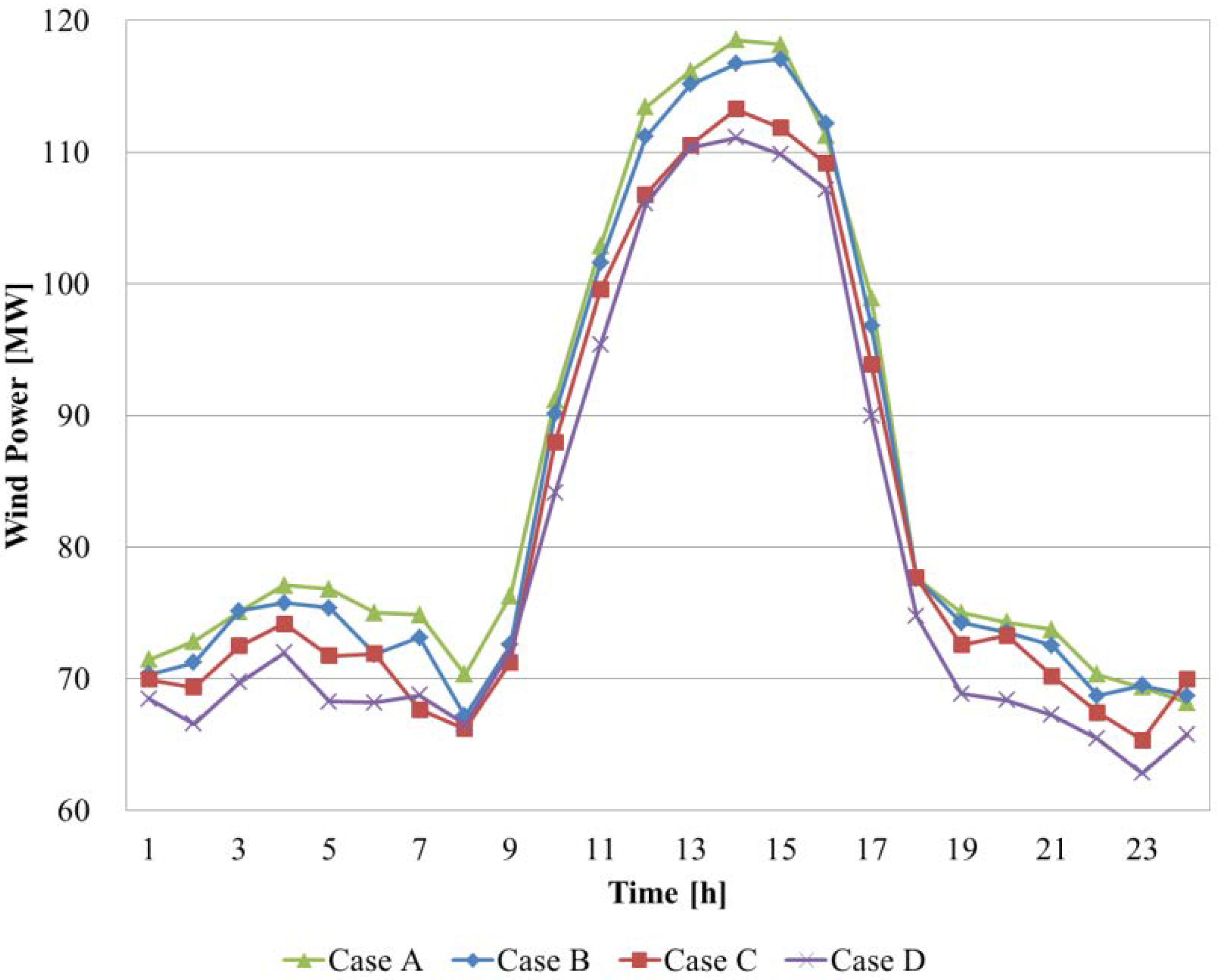
5.3. Wake Effect Depending on Wind Farm Layout
- Case A: no wake effect considered;
- Case B: five wind turbines in a row (WF1: 5 × 8, WF2: 5 × 12);
- Case C: ten wind turbines in a row (WF1: 10 × 4, WF2: 10 × 6);
- Case D: twenty wind turbines in a row (WF1: 20 × 2, WF2: 20 × 3).
| Case | Total operating cost ($) | Wind power generation | ||
|---|---|---|---|---|
| P (MW) | Q (MVar) | CP (%) | ||
| A | 2,330,318 | 2,043 | 420 | 28.3 |
| B | 2,331,503 | 2,017 | 417 | 28.0 |
| C | 2,333,823 | 1,963 | 408 | 27.2 |
| D | 2,335,079 | 1,907 | 404 | 26.4 |
6. Conclusions
Nomenclature:
| i | Index for bus |
| t | Index for time period |
| n | Index for wind farm |
| m | Index for wind turbine |
| NG | Number of units |
| NWT,n | Number of wind turbines in n-th wind farm |
| Nc | Number of contingencies |
| NWF | Number of wind farms |
| NB | Number of buses |
| NT | Number of time period |
| ai,bi,ci | Coefficients of the quadratic production cost function of unit i |
| αi,βi,γi,ζi,λi | Coefficients of the CO2 emission function of unit i |
| f(·) | Probabilistic distribution function |
| V | Random variable of wind speed |
| v | Wind speed considering wake effect |
| v0 | Free wind speed |
| vin | Cut-in speed |
| vr | Wind turbine rated speed |
| vout | Cut-out speed |
| Pi | Power output of thermal generating unit i |
| PD | Power load |
| PL | Transmission network losses of system |
| PW(v)n,m | Generated wind power from m-th wind turbine of n-th wind farm |
| μPD | Mean value of power load |
| σPD | Standard deviation of power load |
| μV | Mean value of wind speed |
| σV | Standard deviation of wind speed |
| cov1,2 | Covariance of between two wind speed series |
| c | Scale factor of Weibull distribution |
| k | Shape factor of Weibull distribution |
| y | Correlated Weibull random variable vectors |
| L | Cholesky decomposition matrix |
| d | Wake deduction coefficient |
| Ct | Thrust coefficient of wind turbine |
| Cp | Power coefficient of wind turbine |
| w | Wake decay constant |
| x | horizontal distance behind the upstream turbine |
| D | Wind turbine blade diameter |
| Z | Vector of the decision variables Z = [U X]T |
| X | Vector of the state variables (V, θ) |
| U | Vector of the control variables (P, Pwt, pf) |
| f | Objective function representing the system operating costs |
| G(∙), H(∙) | Vector function representing the equality constraints and the inequality constraints, respectively |
| Hmin, Hmax | Lower and upper limits of the inequality constraints vector, respectively |
Acknowledgments
Conflicts of Interest
References
- Xie, L.; Carvalho, P.M.S.; Ferreira, L.A.F.M.; Liu, J.; Krogh, B.H.; Popli, N.; Ilic, M.D. Wind integration in power systems: Operational challenges and possible solutions. IEEE Proc. 2011, 99, 214–232. [Google Scholar]
- Tuohy, A.; Meibom, P.; Denny, E.; O’Malley, M. Benefits of Stochastic Scheduling for Power Systems with Significant Installed Wind Power. In Proceedings of the 10th International Conference on Probabilistic Methods Applied to Power Systems (PMAPS), Rincon, PR, USA, 25–29 May 2008; pp. 1–7.
- Wang, J.; Botterud, A.; Bessa, R.; Keko, H.; Carvalho, L.; Issicaba, D.; Sumaili, J.; Miranda, V. Wind power forecasting uncertainty and unit commitment. Appl. Energy 2011, 88, 4014–4023. [Google Scholar]
- Ummels, B.C.; Gibescu, M.; Pelgrum, E.; Kling, W.L.; Brand, A.J. Impacts of wind power on thermal generation unit commitment and dispatch. IEEE Trans. Energy Convers. 2007, 22, 44–51. [Google Scholar] [CrossRef]
- Tuohy, A.; Meibom, P.; Denny, E.; O’Malley, M. Unit commitment for systems with significant wind penetration. IEEE Trans. Power Syst. 2009, 24, 592–601. [Google Scholar] [CrossRef]
- Ruiz-Rodriguez, F.; Hernández, J.; Jurado, F. Probabilistic load flow for photovoltaic distributed generation using the Cornish–Fisher expansion. Electr. Power Syst. Res. 2012, 89, 129–138. [Google Scholar] [CrossRef]
- Holttinen, H. Hourly wind power variations in the Nordic countries. Wind Energy 2005, 8, 173–195. [Google Scholar] [CrossRef]
- Feijóo, A.; Villanueva, D.; Pazos, J.L.; Sobolewski, R. Simulation of correlated wind speeds: A review. Renew. Sustain. Energy Rev. 2011, 15, 2826–2832. [Google Scholar] [CrossRef]
- Gao, Y.; Billinton, R. Adequacy assessment of generating systems containing wind power considering wind speed correlation. IET Renew. Power Gener. 2009, 3, 217–226. [Google Scholar] [CrossRef]
- Usaola, J. Probabilistic load flow with correlated wind power injections. Electr. Power Syst. Res. 2010, 80, 528–536. [Google Scholar] [CrossRef]
- Barthelmie, R.; Pryor, S. An overview of data for wake model evaluation in the Virtual Wakes Laboratory. Appl. Energy 2013, 104, 834–844. [Google Scholar] [CrossRef]
- Feijoo, A.E.; Cidras, J. Modeling of wind farms in the load flow analysis. IEEE Trans. Power Syst. 2000, 15, 110–115. [Google Scholar] [CrossRef]
- Petru, T.; Thiringer, T. Modeling of wind turbines for power system studies. IEEE Trans. Power Syst. 2002, 17, 1132–1139. [Google Scholar] [CrossRef]
- Martinez-Rojas, M.; Sumper, A.; Gomis-Bellmunt, O.; Sudrià-Andreu, A. Reactive power dispatch in wind farms using particle swarm optimization technique and feasible solutions search. Appl. Energy 2011, 88, 4678–4686. [Google Scholar] [CrossRef]
- Nian, H.; Quan, Y.; Hu, J. Improved control strategy of DFIG-based wind power generation systems connected to a harmonically polluted network. Electr. Power Syst. Res. 2012, 86, 84–97. [Google Scholar] [CrossRef]
- Engelhardt, S.; Erlich, I.; Feltes, C.; Kretschmann, J.; Shewarega, F. Reactive power capability of wind turbines based on doubly fed induction generators. IEEE Trans. Energy Convers. 2011, 26, 364–372. [Google Scholar] [CrossRef]
- Rabelo, B.C.; Hofmann, W.; da Silva, J.L.; de Oliveira, R.G.; Silva, S.R. Reactive power control design in doubly fed induction generators for wind turbines. IEEE Trans. Ind. Electron. 2009, 56, 4154–4162. [Google Scholar] [CrossRef]
- Villanueva, D.; Feijóo, A.; Pazos, J.L. Probabilistic load flow considering correlation between generation, loads and wind power. Smart Grid Renew. Energy 2011, 2, 12–20. [Google Scholar] [CrossRef]
- Hagspiel, S.; Papaemannouil, A.; Schmid, M.; Andersson, G. Copula-based modeling of stochastic wind power in Europe and implications for the Swiss power grid. Appl. Energy 2012, 96, 33–34. [Google Scholar] [CrossRef]
- Morales, J.M.; Minguez, R.; Conejo, A.J. A methodology to generate statistically dependent wind speed scenarios. Appl. Energy 2010, 87, 843–855. [Google Scholar] [CrossRef]
- Mortensen, N.G.; Heathfield, D.N.; Myllerup, L.; Landberg, L.; Rathmann, O.; Troen, I.; Petersen, E. Getting Started with WAsP8; Risø National Laboratory: Roskilde, Denmark, 2003. [Google Scholar]
- Liu, X.; Xu, W. Minimum emission dispatch constrained by stochastic wind power availability and cost. IEEE Trans. Power Syst. 2010, 25, 1705–1713. [Google Scholar] [CrossRef]
- Capitanescu, F.; Glavic, M.; Ernst, D.; Wehenkel, L. Interior-point based algorithms for the solution of optimal power flow problems. Electr. Power Syst. Res. 2007, 77, 508–517. [Google Scholar] [CrossRef]
- Wei, H.; Sasaki, H.; Kubokawa, J.; Yokoyama, R. An interior point nonlinear programming for optimal power flow problems with a novel data structure. IEEE Trans. Power Syst. 1998, 13, 870–877. [Google Scholar] [CrossRef]
- Yamin, H.; Al-Tallaq, K.; Shahidehpour, S. New approach for dynamic optimal power flow using Benders decomposition in a deregulated power market. Electr. Power Syst. Res. 2003, 65, 101–107. [Google Scholar] [CrossRef]
© 2013 by the authors; licensee MDPI, Basel, Switzerland. This article is an open access article distributed under the terms and conditions of the Creative Commons Attribution license (http://creativecommons.org/licenses/by/3.0/).
Share and Cite
Lyu, J.-K.; Heo, J.-H.; Park, J.-K.; Kang, Y.-C. Probabilistic Approach to Optimizing Active and Reactive Power Flow in Wind Farms Considering Wake Effects. Energies 2013, 6, 5717-5737. https://doi.org/10.3390/en6115717
Lyu J-K, Heo J-H, Park J-K, Kang Y-C. Probabilistic Approach to Optimizing Active and Reactive Power Flow in Wind Farms Considering Wake Effects. Energies. 2013; 6(11):5717-5737. https://doi.org/10.3390/en6115717
Chicago/Turabian StyleLyu, Jae-Kun, Jae-Haeng Heo, Jong-Keun Park, and Yong-Cheol Kang. 2013. "Probabilistic Approach to Optimizing Active and Reactive Power Flow in Wind Farms Considering Wake Effects" Energies 6, no. 11: 5717-5737. https://doi.org/10.3390/en6115717