A Self-Adapting Approach for Forecast-Less Scheduling of Electrical Energy Storage Systems in a Liberalized Energy Market

Abstract

In this paper, an original scheduling approach for optimal dispatch of electrical Energy Storage Systems (ESS) in modern distribution networks is proposed. The control system is based on fuzzy rules and does not use forecasts since it repairs the past history according to the real time data on the electrical energy cost, renewable energy production and load. When the system detects a worsening of performances, the fuzzy logic rule-based control system self-adapts its membership functions using an economic indicator. The common use, in the relevant literature, of forecasted values in such systems can lead to large errors and economic losses. Moreover the speed of calculation guaranteed by the fuzzy control system allows the execution of new calculations even with high frequency. After the Introduction section, where the state of the art on the topic is outlined, the problem formulation is presented and an interesting application of the considered approach to the control on a medium size battery with real world data is proposed.

1. Introduction

The problem of optimal scheduling of Distributed Energy Resources, DER, in modern distribution systems is a quite studied subject in the literature [1,2,3,4,5,6]. Generally speaking the problem of scheduling can be defined by a set of tasks and a set of resources. Tasks are constrained by precedence relationships, which bind some tasks to wait for other ones to complete before they can start. The goal is to find a schedule that performs all tasks optimally (minimum time, maximum profit, etc.). In this case, the term scheduling is used extensively to represent the problem of optimal economic dispatch of the energy resource stored in an Electrical Storage System (ESS) serving a load and a Renewable Energy Source (RES) generation unit. The tasks in this case are the charge and discharge cycles and the precedence relationships of such tasks depend on the needed availability of energy in the present and in the following time intervals.

In the power distribution area, most scheduling problems rely on forecasts of the parameters that will affect the behavior of the dispatched system. And in the same way to solve the issue, especially referring to ESS, almost all papers rely on forecasts of the loads course, of energy prices and of RES production. The increasing sudden weather changes make forecasts on production from RES ever more unreliable, thus leading to the analysis of tools to cope with such uncertainty.

The problem formulation also depends on the market environment and to the degree of participation of the energy resources to the market. It is indeed well known that the energy market clearance takes place at different times:

• Day Ahead Market (DAM);
• Hour Ahead Market (HAM);
• Real Time Market (RTM, balancing services).

The DAM is a forward market in which prices are calculated based on the time scheduling of the subsequent first business day. The DAM creates the basis for the other markets. In this market, the hourly prices are determined at the points where demand and offer meet. The HAM makes the balance between production and consumption. It can be used to sell/buy the quantities that have not been dealt with during the auction or unplanned maintenance after the auction. It is a flexible tool also used for arbitrage with neighboring countries. The RTM is a spot market in which current prices are calculated in very short time (order of minutes, usually 5 min) according to the actual operating conditions of the network. It is a balancing market for the security of the system: it is aimed at managing congestion in real time after that all other processes have been carried out, to balance the demand instantaneously, to reduce the supply if demand falls. It provides ancillary services as needed.

In all cases, the market uses energy prices that reflect the value of the energy of the place and depends on the specific supply source: demand and offer meet and the price is determined based on the availability of energy and of the existing infrastructures.

Typically what happens is that each prosumer (producer and consumer) commits itself for a given amount of energy (bought or sold) according to forecasts. Otherwise, the prosumer does not take part to the market and simply buys and/or sells the energy locally at a price that can either be fixed in different times of the day or variable according to the real time market.

Dispatchable sources from renewable generators can be created installing Energy Storage Systems (ESS). In fact, an ESS can be suitably controlled in order to dispatch the energy generated from the renewable source according to an economic criterion [7,8]. An innovative device for this purpose has been proposed in [9,10].

In the Day Ahead and Hour Ahead markets, the objective of the scheduler of an ESS would be that to support the promises of purchase or selling by the different actors compensating the uncertainties that may arise. In the Real Time Market, the aim is that to maximize the profit or limit the costs of the actors or cover the relevant needs in real time.

If an ESS instead serves a small or medium size customer, typically the objective will be that to limit the expenses trying to follow tariffs that can either be Time of Use (TOU) or Real Time Pricing (RTP). The most common approach is that to use forecasts to generate a suitable schedule for the storage system charge controller.

Costa et al. [11] and Dicorato et al. [12] proposed a scheduling of wind installation + ESS to get the possible maximum profit and focus mainly on the energy market clearance at day ahead market. To have the scheduling of wind installation + ESS, wind power generation has to be predicted, obtaining a long-term forecast Pf (t). However, given the non-controllable and stochastic nature of the wind or solar resources, using suitable predictions to obtain accurate forecast is difficult thus leading to possible errors, especially for long-term prediction.

A proposal of using Model Predictive Control (MPC) to obtain a scheduling of RES + ESS based on real-time measures is given in [13,14,15,16]. The use of MPC has decreased the errors caused by long-term forecasts, but not entirely eliminated the problem. Pérez et al. [16] admitted that: “the main drawbacks of MPC are the need for accurate prediction model of the controlled outputs and the computational effort required to solve a constrained optimization problem, which can be too consuming for fast process applications”.

Sometimes, the uncertainty about forecasts is included in the problem formulation [17] where the optimization takes into account the cost associated to the worst case scenario.

On the contrary, in this paper the real-time scheduling of a RES system + ESS created by a forecast-less charge controller for ESS is proposed. The approach does not need extensive calculation because it is model free. And as other model-free optimization approaches it can provide a control action in a very short calculation time [18,19].

A similar approach was proposed by Manjiljr et al. [20] where a fuzzy controller was also designed to cope with real time pricing of energy. The approach is however lacking of any mechanism to deal with possible price course variations, and technical constraints concerning the lifetime of batteries preservation sizing is not managed within the control system.

To deal with the stochastic nature of the parameters involved and to the inherent uncertainty of the problem when using weather forecasts as inputs the authors propose the use of Stochastic Linear Programming in [21].

Also there is no self-adaptation mechanism to adjust the fuzzy control system’s parameters to the current situation. In [22] the Authors investigate the possibility to use a new modeling of Energy Storage Systems based on zero integral functions (namely a function whose integral in a given time interval is null). Such functions are well suited to represent the course of the variation of energy level stored in batteries during the solution of optimal management problems in smart-grids.

Besides, in order to meet the constraint of finite capacity of the ESS, if the parameters affecting the ESS operation can be considered unchanged from one day to the other (with a period of 24 h), the variation of the State of Charge (SOC) of the ESS along 24 h must be zero. The variation of the SOC is the integral of the output/input power from the ESS.

2. Studied System

The considered scenario consisting of a single aggregate of prosumers that can buy energy locally at a price that varies in real time. The load can either be supplied by the main grid or by the ESS + RES.

In Figure 1, the ESS fuzzy controller implements a rolling horizon scheduler [23,24] using a fuzzy rule based system that repairs the past history to meet objectives and constraints. For a technically feasible solution for the ESS controller the solution proposed in [25] can be employed.

Figure 1. Studied system.

Figure 1. Studied system.

In the proposed application the objectives to be achieved are:

• to limit the power purchase during the high price hours;
• to increase the power purchase during the low price hours;
• to control the charge and discharge operation so as not to exceed the ESS size;
• to limit the number of charge and discharge cycles, to preserve the lifetime of batteries.

The ESS is thus managed considering constraints over its finite capacity of storing energy and over the maximum number of maneuvers that can be carried out in a considered time interval. The price signals coming from the energy market influence the ESS fuzzy controller. In the considered scenario, the ESS injects power on the DC bus and does not inject power into the main grid. The controller is provided with a self-adaptation mechanism allowing the fine tuning of the fuzzy controller parameters in order to cope with the inevitable changes in the energy price course.

For clarity it will be assumed that the RES based unit is a photovoltaic generation unit, PV, although any type of non dispatchable generation system could be as well considered. In the following sections, first the basic architecture of a Rolling horizon scheduler is described, then the fuzzy controller and the self-adaptation mechanism are detailed. Finally, the application section shows the effectiveness of the proposed approach with some interesting applications.

3. Measures to Fix Uncertainty in ESS Scheduling Based on the Rolling Horizon Approach

One of the weakest points in optimally allocating resources in the time to come is the need of forecasts. Scheduling is indeed the problem of optimally allocating resources in a limited timeframe. Therefore predictions are fundamental to carry out such operation. In the literature, the extreme complexity of the considered issue, also considering different time horizons for the different Markets, has been addressed by identifying a hierarchy of time horizons (medium-term or yearly, weekly, daily, hourly) in which was progressively refined the model of the system and enriched the set of technical constraints to be taken into account.

When the dispatch problem formulation depends on forecasts related to highly unpredictable phenomena, such as weather dynamics (i.e., sun irradiation and wind intensity) it is required to account for it. This is the case of Energy Resources scheduling in modern power distribution systems, where large amounts of RES are installed. In these systems, though, efficient scheduling approaches minimizing the uncertainty deriving from forecasts have been proposed by different authors. Looking at the previous work in the scheduling area [23], some interesting approaches can be taken. As an example, rolling horizon algorithms [24] try to cope with the problem of uncertain predictions. Rolling horizon approaches are efficient scheduling techniques and are a common business practice for making decisions in a stochastic dynamic environment. In essence, this practice involves making the most immediate decisions based on a forecast of relevant information for a certain number of time intervals in the future. Once the first period decision is taken, the second period decision is to be devised. In this case, forecasts for additional periods in the future may be required and existing forecasts may be updated.

The approach consists of breaking the entire scheduling horizon into sub-scheduling intervals characterized by a given a re-scheduling frequency. These methods are also characterized by:

• a sub-scheduling horizon, fixing part of the operations to schedule;
• a rescheduled horizon, fixing the part of the preceding schedule carried over to the new schedule.

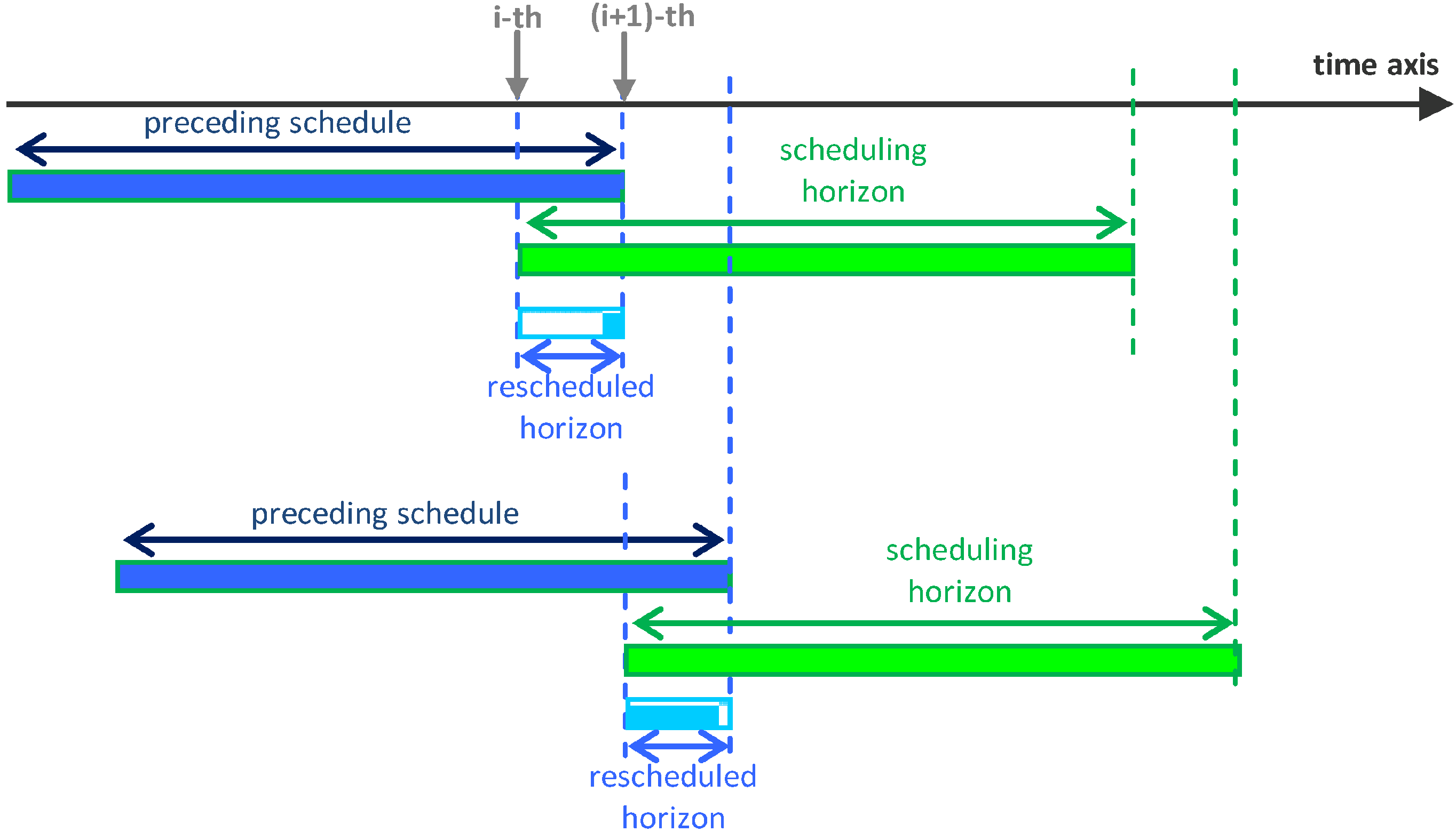
Figure 2 shows the principle behind the rolling horizon algorithm. The rescheduled horizon is a part of the schedule that is re-planned as a part of schedules outputted in preceding time, it therefore overlaps with the new plan and is re-scheduled.

Figure 2. The rolling horizon algorithm.

Figure 2. The rolling horizon algorithm.

In Figure 2, showing the rolling horizon algorithm in two consecutive time step i and i + 1, the grey arrows indicating the current (i) and the immediately subsequent (i + 1) times. The most interesting applications of the rolling horizon algorithms in highly unpredictable environments are the online application where such rescheduling is carried out according to real time input data.

According to some interesting papers on the subject, the rolling horizon approach continuously repairs the schedule adapting it to the newly arrived forecasts and real time data [26].

It seems, however, that even with rolling horizon approaches [3,26] forecasts are needed. There are also a couple of problem-related motivations for which the use of forecasts in scheduling problems are needed:

(1)

When there is a constraint linking the optimization variables in a given time horizon. When indeed the action to be taken in the following elementary time interval does not influence the future actions, the prediction of future values of the parameters is not necessary;

(2)

When the schedule is needed to create an offer of goods or services to third parties. In this case, as in the energy market, the schedule of power generated from a given unit is a basic element on which the negotiations can take place.

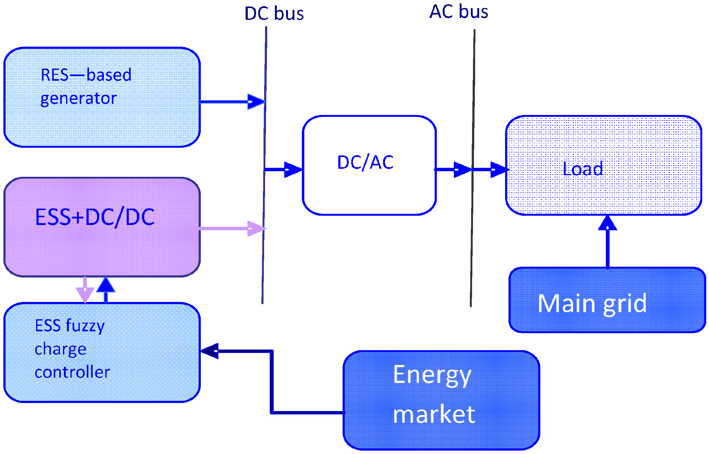
In the case under study, described in Figure 1, condition (2) may not hold because the prosumer only uses real time data coming from the market. Indeed, in this case, signals coming from the real-time market, measured loads and power production from the RES are used as inputs for the controller of the ESS. The latter, also on the basis of the previous behavior, decides the action to be taken over the ESS (whether to charge or discharge, and at what rate) in the current elementary time interval (eti).

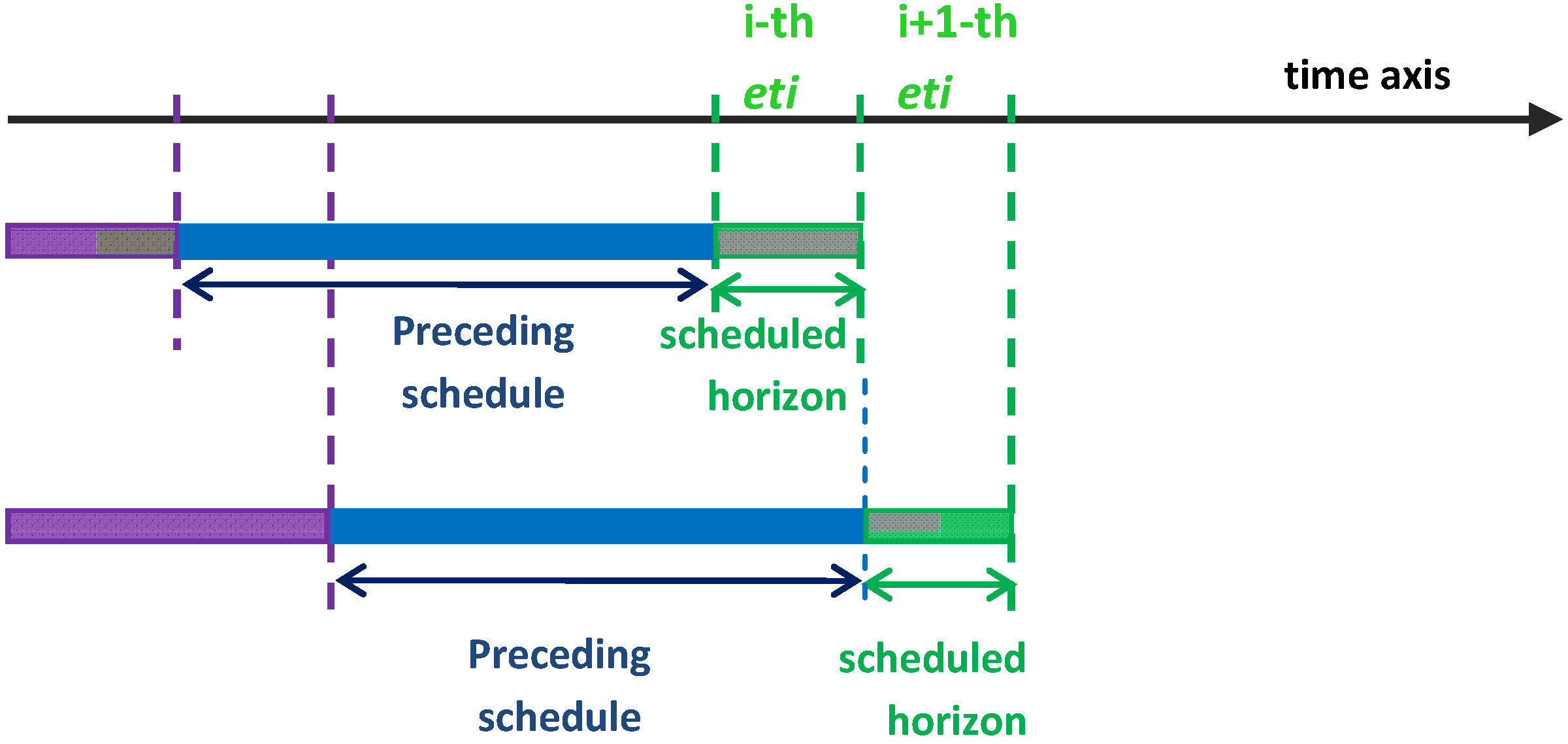
Figure 3 shows the principle behind the proposed forecast-less rolling horizon approach proposed in this paper. In the figure, the elementary time interval, eti, is depicted in a green segment; the time interval used to decide what action to take is represented in blue, while the purple segment represents the time interval no longer useful for future decisions. Differently from standard rolling horizon approaches the schedule to be repaired is the backward schedule, due to the specific feature of the resource to be managed (energy stored in a battery).

Figure 3. The proposed forecast-less rolling horizon approach.

Figure 3. The proposed forecast-less rolling horizon approach.

In the proposed approach, indeed, the past is considered as a schedule to be repaired, when the parameters affecting the desired behavior change, using the action to be determined in the following eti. The latter control action can be modified to meet the posed objectives and repair possible constraints violations or deviations from economic benefit. In absence of forecasts for future times, the horizon to be rescheduled is thus only the following eti.

As described, the approach appears conservative since it may not allow one to take risks that can possibly be repaired in the future and that can also provide high returns. Nonetheless, the applications section will show that this depends on the choice of a suitably adaptable control algorithm for the ESS controller and on its capacity to self-adapt to the mutated external conditions. In this paper, the control algorithm is a Fuzzy Rule-Based System (FRBSs), that will be described in the following section.

It is well known that the most important implementation of Fuzzy Set Theory [27,28,29,30] are FRBSs. These systems are an extension of classical Rule-Based Systems, since they use fuzzy rules instead of classical logic rules. Thanks to their property to successfully manage different types of control problems, they have been applied to a wide range of problems from different fields showing uncertainty and vagueness in different ways [31,32,33,34]. For standard rule-based systems, a FRBS is composed of:

(1)

The Inference System, which puts into effect the fuzzy inference process needed to obtain an output from the FRBS when an input is specified;

(2)

The Knowledge Base (KB) representing the knowledge known about the problem being solved, constituted by a collection of fuzzy rules. The rules are designed to produce a desired behavior.

Such behavior can be summarized in a few sentences:

in a stable situation, the energy stored and released over a predefined number, T_E, of elementary time intervals should tend to zero (SOC variation, Δ_SOC);

when the price of energy is high, release energy, when it is low, store energy.

The two conditions above describe a desirable behavior for an ESS serving a load and a RES based generation plant, provided the number of charge and discharge maneuvers over T_E elementary time intervals is limited below a given number n_m. Since the rolling horizon width is of 24 h and the sampling rate is 1/h, in our application T_E is 24 and eti is 1 h. These sentences can be combined together to create a FRBS. The fuzzy rules are summarized in Table 1 below.

Table 1. Fuzzy rules for the energy storage systems (ESS) charge controller.

Membership functions: Price and ΔSOC	Price low	Price medium	Price high
ΔSOC low	Charge	Charge	Stand-by
ΔSOC medium	Charge	Stand-by	Discharge
ΔSOC high	Stand-by	Discharge	Discharge

Table 1. Fuzzy rules for the energy storage systems (ESS) charge controller.

Membership functions: Price and ΔSOC	Price low	Price medium	Price high
ΔSOC low	Charge	Charge	Stand-by
ΔSOC medium	Charge	Stand-by	Discharge
ΔSOC high	Stand-by	Discharge	Discharge

The notions of “high” and “low” referred to prices are not clearly defined. For this reason, the uncertainty has been expressed through membership functions for the linguistic values “low”, “medium” and “high” of the linguistic variable Price. The membership function expressing the medium value has been centered on the average value of the energy prices over the preceding T_P hours. Also the notion of “low”, “medium” and “high” referred to the variation of the State Of Charge, Δ_SOC is not trivial. A too strict implementation of the notion of “high” and “low” would lead to unstable behavior, while a too loose implementation would produce an undesired behavior not meeting condition (a). However, the system is designed in a way that it can learn from its own experience on the field adjusting the membership functions parameters according to an indicator measuring the profit attainable by selling/buying energy. Every time the system experiences a loss of profit in a reference timeframe (i.e., 24 h), it adjusts its own parameters simply shifting the membership functions, otherwise it keeps the same parameters. In the following section, the fuzzy controller, the choice of the membership functions, the inference mechanism and the self-adaptation technique are described in greater details.

3.1. The Membership Functions

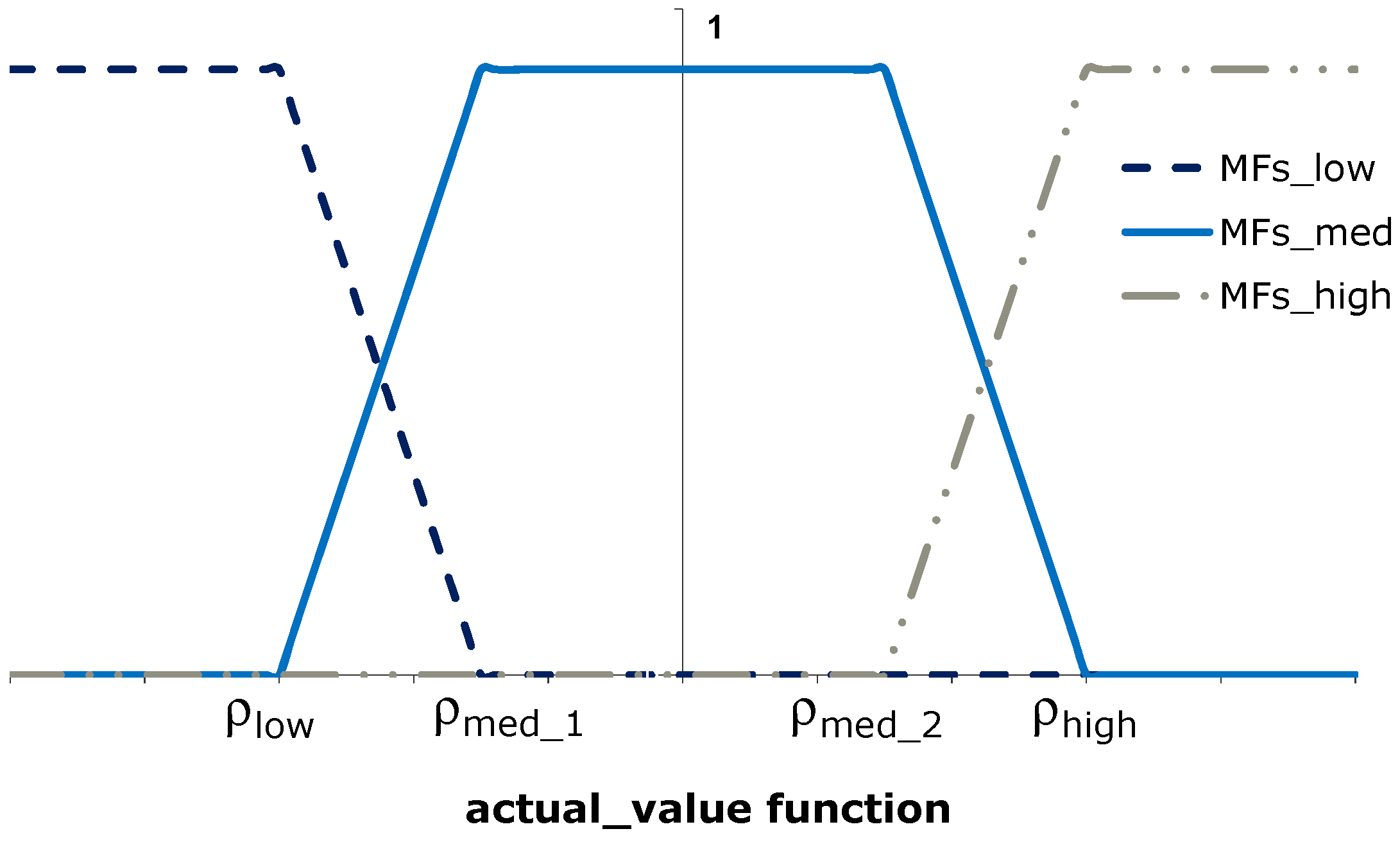
The most commonly adopted shapes of Membership Functions (MFs) have been tried. Firstly, trapezoidal MFs, have been tried, like those represented in Figure 4; for each of the quantities SOC and Price, they are characterized by 4 parameters: ρ_low for MFs_low curve, ρ_high for MFs_high curve, ρ_med-1 and ρ_med-2 for MFs_med curve.

Figure 4. Trapezoidal membership functions (MFs).

Figure 4. Trapezoidal membership functions (MFs).

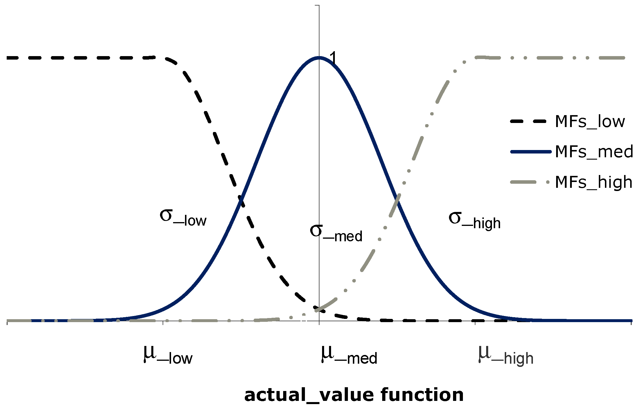
However, more reliable results were obtained using Gaussian shapes characterized by six parameters (average “μ” and standard deviation “σ” for each curve MFs_low, MFs_med, MFs_high) as represented in Figure 5. Due to a richer representation and a better possibility of fine tuning, more satisfactory results were attained.

Figure 5. Gaussian membership functions (MFs).

Figure 5. Gaussian membership functions (MFs).

3.2. The Inference Mechanism

In the FRBS, the rules outlined in Table 1 are activated all together and the AND-min operator has been used to infer the consequent. Then the consequents of the rules are combined through the OR-max leading to the action to be taken by the ESS controller. As it is evident from Table 1, the consequents of the rules are actions taken over the ESS. Their degree of specialization according to the situation presented to the FRBS is measured by the result of the inference. Namely the defuzzification is simply carried out taking the most specific rule (the rule showing the highest consequent) and taking its outcome action (charge/discharge/stand-by). In order to preserve the batteries life time due to an excessive number of maneuvers, the control action is subjected to a verification on the past history also looking at the number of operations carried out over the battery in the last T_m hours. In the considered timeframe, T_m, a maximum number of maneuvers was thus fixed, n_m, that was compared to the current number of maneuvers carried on the ESS after the currently decided control action.

If such comparison gives a negative outcome the maneuver is not carried out.

A maneuver is intended as:

• if battery moves from charge to discharge state or;
• if the battery moves from discharge to charge state.

In some cases, even if the constraint above is violated, the state of the battery must move to the stand by position, because the SOC in the battery is close to zero or is at the maximum level.

The rate P_batt(i) at which charge and discharge are carried out is constant for all eti (indicated with i), considering the charge and discharge efficiency, η, as a factor below the unity, it follows the rule:

$$P_{batt}(i)=\eta \cdot P_{out}$$

(1)

where P_out has been calculated dividing the size of the battery C_batt by the time taken to complete a full charge of the ESS.

When the ESS is close to full charge or to complete discharge, it may be impossible to inject/absorb P_batt(i) as defined above. In these cases, P_batt(i) will take a different value according to the available energy stored in the battery, if close to full discharge or according to the available space for storing energy, if close to full charge. Therefore, P_batt(i) will take values according to the following relations:

during charge and close to full charge:

$$P_{batt}(i)=- {\frac{C_{batt}-SOC(i)}{eti}|}_{\left(C_{batt}-SOC(i)\right)/eti < \eta \cdot P_{out}}$$

(2)

during discharge and close to full discharge:

$$P_{batt}(i)= {\frac{SOC(i)}{eti}|}_{SOC(i)/eti < \eta \cdot P_{out}}$$

(3)

where eti is the width of the elementary time interval (i.e., 1 h) and SOC(i) is the State of Charge at the i-th eti.

3.3. The Self-Adaptation Technique

When the system experiences an economic loss over a predefined timeframe (i.e., 24 h), the MFs parameters are adjusted.

The economic loss is evaluated by comparing the cost of energy required to supply the load E_load(i) [also considering the energy supplied by the RES unit E_PV(i)] in the last 24 h in absence of an ESS and in presence of an ESS with the considered FRBS controller.

Indicating with Price(i) the real time price of electrical energy in the i-th eti, the cost of energy to supply the load can be expressed as follows:

in absence of ESS:

$$\text{cos}t(i)=Price(i)\cdot \left(E_{load}(i)-E_{PV}(i)\right)$$

(4)

in presence of ESS:

$$\text{cos}t(i)=Price(i)\cdot \left(E_{load}(i)-E_{PV}(i)-{\mathrm{\Delta }}_{SOC}(i)\right)$$

(5)

where ${\Delta }_{SOC}$ (i) is the Energy supplied/absorbed by the ESS in the i-th elementary time interval eti.

$${\mathrm{\Delta }}_{SOC}(i)=P_{batt}(i)\cdot eti$$

(6)

At each eti, the system tries to improve its operating conditions (the value of MFs parameters) using as indicator the economic benefit calculated over the last 24 h:

$$\mathrm{\Delta }Cost(i)={\displaystyle \sum _{j=(i-24)}^{i}Price(j)\cdot P_{batt}(j)}<0$$

(7)

If the system experiences an economic loss in previous 24 h, it will try to improve the situation by applying a random mutation of the MFs parameters.

A random adjustment of the MFs parameters is carried out by evaluating, for each mutation carried out on the parameters set, the improvement that there would have been adopting the mutated parameters over the last T_E eti, using the quantity in Equation (7). The mutation is random with uniform distribution between ±10% of the current value.

4. Application and Results

In this section, an application for a medium size ESS, is proposed. The EES has been sized according to the data recorded for a real world system composed of a photovoltaic system and a large residential load.

The studied system characteristics are:

• Peak Load: 0.094 MW;
• Size PV plant: 0.02 MW;
• Size ESS: 0.02 MWh.

The PV plant installation capacity is certainly inadequate to cover the load demand and this is often the case in practice, since there is not enough land to install an adequately sized PV generator.

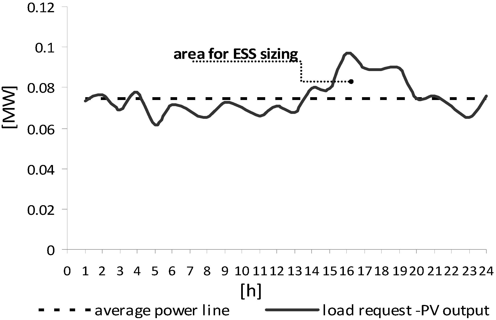
To prove the efficiency of the proposed management approach following maximum economic benefit and technical feasibility, the ESS has been sized according to a peak reduction criterion, see Figure 6. For a typical daily behaviour, the average power required by the summation of the residential load request and the PV generator output along 24 h has been taken. Then the larger area below the average power line has been assumed to be the size of the ESS, with a security factor of 10%.

Figure 6. Photovoltaic production and load request in 24 h and sizing of ESS.

Figure 6. Photovoltaic production and load request in 24 h and sizing of ESS.

The applications will show:

• the efficiency of the self-adaptation mechanism;
• the performance of the control system with a stable daily course of energy prices along the time frame considered;
• the performance of the system with a varied course of energy prices along the time frame considered.

It is shown that results are in both cases quite satisfactory since the fuzzy system self-adapts to the new situation giving raise to a large increase of revenues. The simulations carried out cover a total time window of 14 days. The time interval elementary eti was set to 1 h. The first 24 h are used to define the initial conditions at the 25th h. The profile of the power supplied/absorbed by the ESS in the first 24 h [P_batt(i), for i =1 to 24] is assigned, consequently the number of manoeuvres is known as well as the initial SOC at the 25th hour. In all simulations, the maximum number of maneuvers in 24 h was set equal to three. At each eti, to verify any constraint violation, this number has been checked over the preceding 24 h. Two scenarios are thus analyzed:

Stable behaviour, refers to a price of energy course that does not vary much in the considered time horizon.

Unstable behaviour, to a price of energy course that does vary in shape and average value in the considered time horizon.

The data for both cases have been taken from the Italian Energy Market available on the web [35]. In all the simulations that follow, the following working hypotheses have been made:

State of Charge at the first hour, SOC_1, at full level (SOC_1 = C_batt);

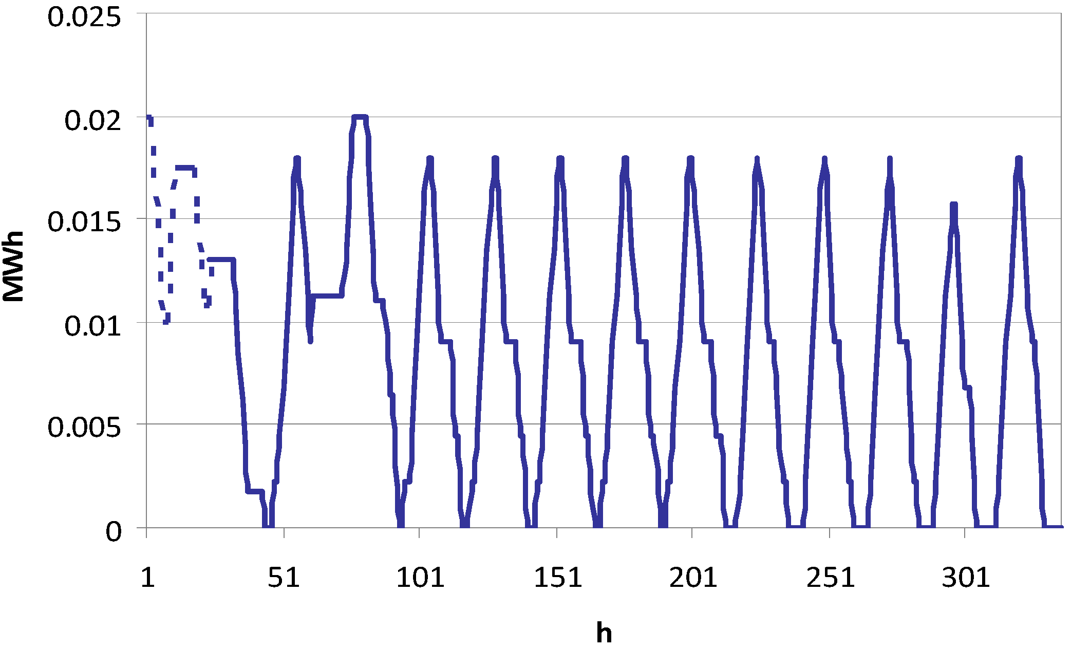
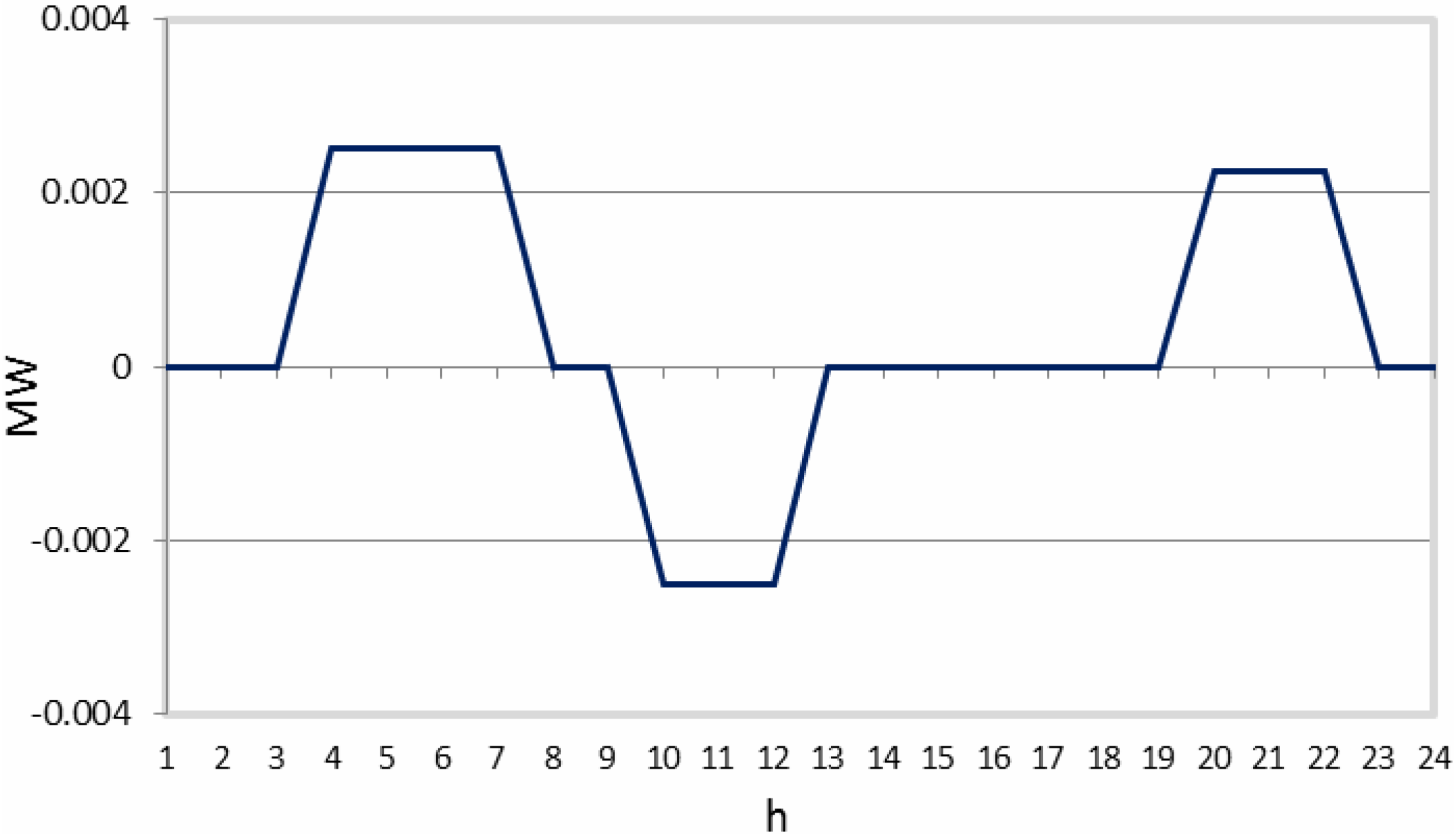
Power injected/absorbed by the ESS, P_batt (i) along the first 24 h, as represented in Figure 7.

Such initial scenario has been chosen, because it is a realistic behavior. Different initial conditions have been also considered; but an appreciable effect on the final result has not been observed with same values of the other parameters.

Figure 7. Power supplied from the battery along the first 24 h of the scheduling horizon.

Figure 7. Power supplied from the battery along the first 24 h of the scheduling horizon.

4.1. Stable Scenario

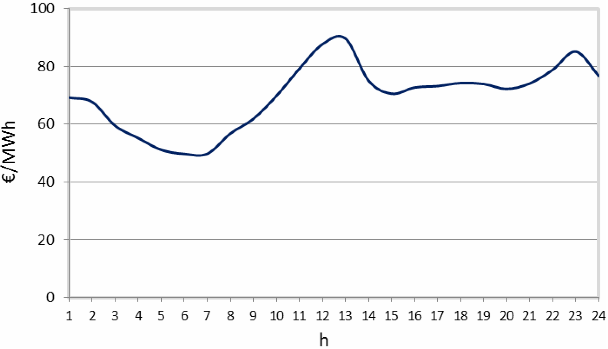
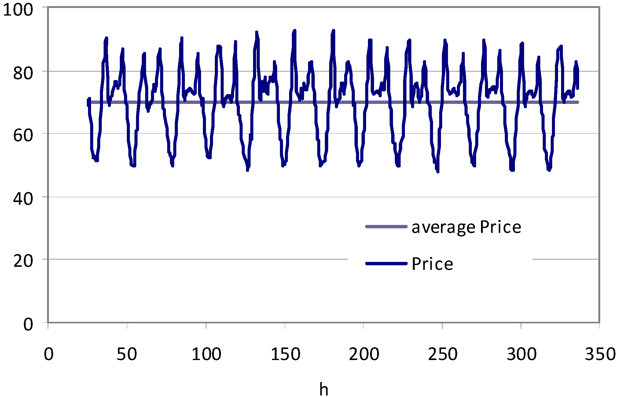
In this set of runs, the following assumption about the price course has been made. The Price was assumed with a stable trend during the two weeks: the price changes at any given time, between different days, does not exceed 5% from the typical average trend shown in Figure 8. Figure 9 shows the price course, and its average value calculated over the previous 24 h.

Figure 8. Daily energy price trend function.

Figure 8. Daily energy price trend function.

Figure 9. Price course along 14 days—stable scenario.

Figure 9. Price course along 14 days—stable scenario.

Figure 10 shows the trend of the power supply Pbatt output by the self-adaptation approach over a stable prices scenario. Figure 11 shows the State of Charge, SOC, of the battery course over the same considered time horizon.

Figure 10. P_batt course along 14 days obtained—stable scenario.

Figure 10. P_batt course along 14 days obtained—stable scenario.

Figure 11. ESS SOC course along 14 days—stable scenario.

Figure 11. ESS SOC course along 14 days—stable scenario.

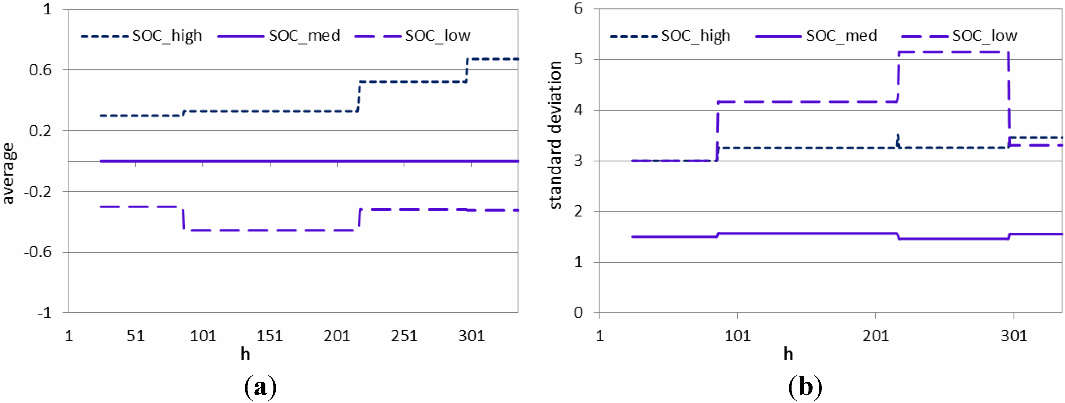
The dotted line in Figure 11 refers to the initial conditions. In the following figures the variations of the parameters of the MFS functions caused by the self-adaptation mechanism are shown. In particular, Figure 12 show the behavior of the average parameters μ (Figure 12a) and the standard deviation parameters σ (Figure 12b) related to Δ_SOC variable. Figure 13a and Figure 13b show the behavior of the same parameters, but related to Price variable.

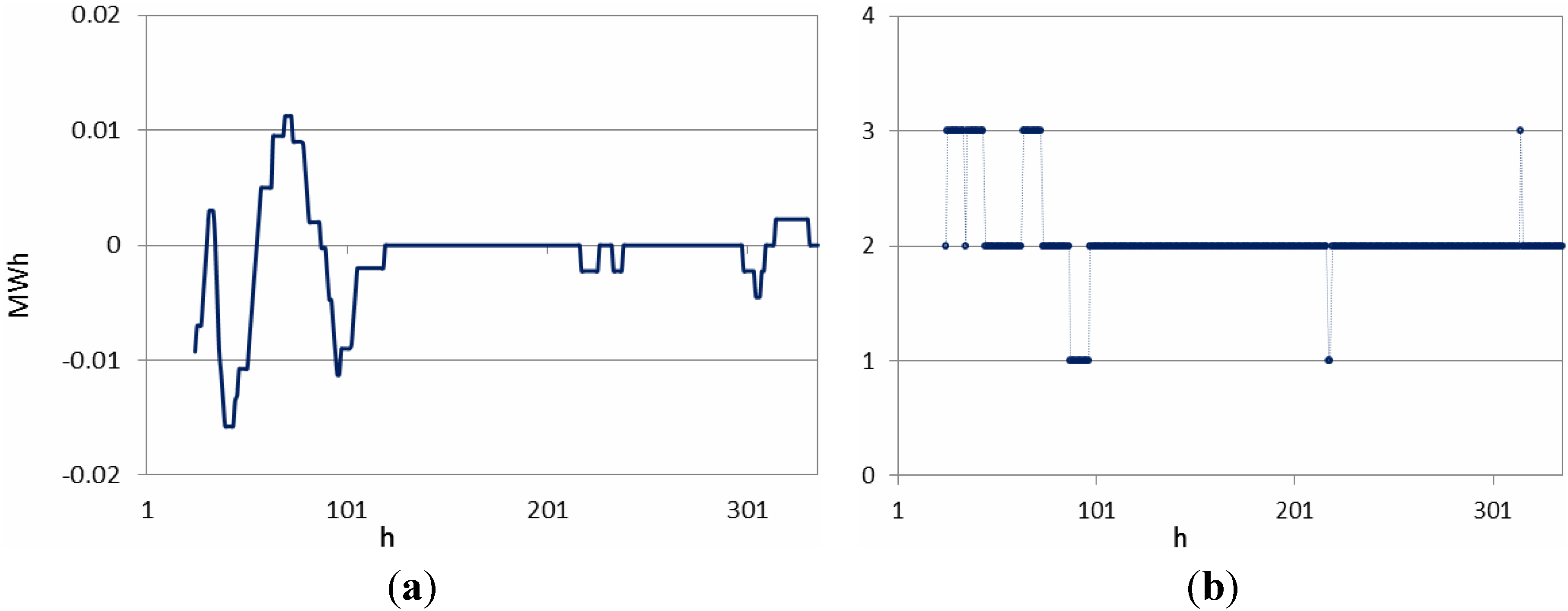
The following Figure 14 shows the value assumed by the technical constraints: the number of maneuvers in the previous 24 h n_m (Figure 14a) and the energy stored and released over the previous 24 h Δ_SOC (Figure 14b). Figure 14a shows that as expected, the value of Δ_SOC calculated over the previous 24 h tends to zero in a stable operating condition. As it can see in Figure 14b, the technical constraints about the number of maneuvers is not violated.

Figure 12. (a) Average parameters μ behaviour for SOC_low, SOC_med and SOC_high MFs and (b) standard deviation parameters σ courses for SOC_low, SOC_med and SOC_high MFs.

Figure 12. (a) Average parameters μ behaviour for SOC_low, SOC_med and SOC_high MFs and (b) standard deviation parameters σ courses for SOC_low, SOC_med and SOC_high MFs.

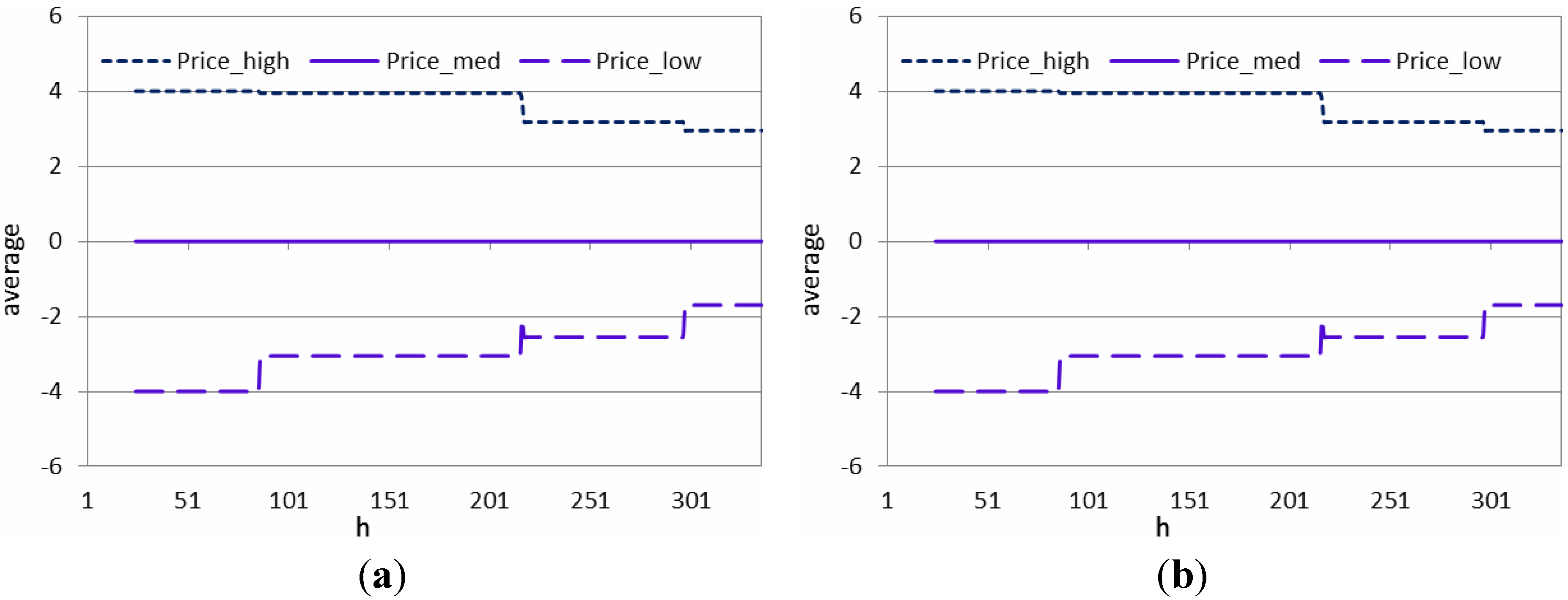
Figure 13. (a) Average parameters μ courses for Price_low, Price_med and Price_high MFs and (b) standard deviation parameters σ courses for Price_low, Price_med and Price_high MFs.

Figure 13. (a) Average parameters μ courses for Price_low, Price_med and Price_high MFs and (b) standard deviation parameters σ courses for Price_low, Price_med and Price_high MFs.

Figure 14. (a) Energy stored and released, Δ_SOC, over the previous 24 h and (b) Number of operations over the battery calculated in each hour within the previous 24 h.

Figure 14. (a) Energy stored and released, Δ_SOC, over the previous 24 h and (b) Number of operations over the battery calculated in each hour within the previous 24 h.

4.2. Unstable Scenario

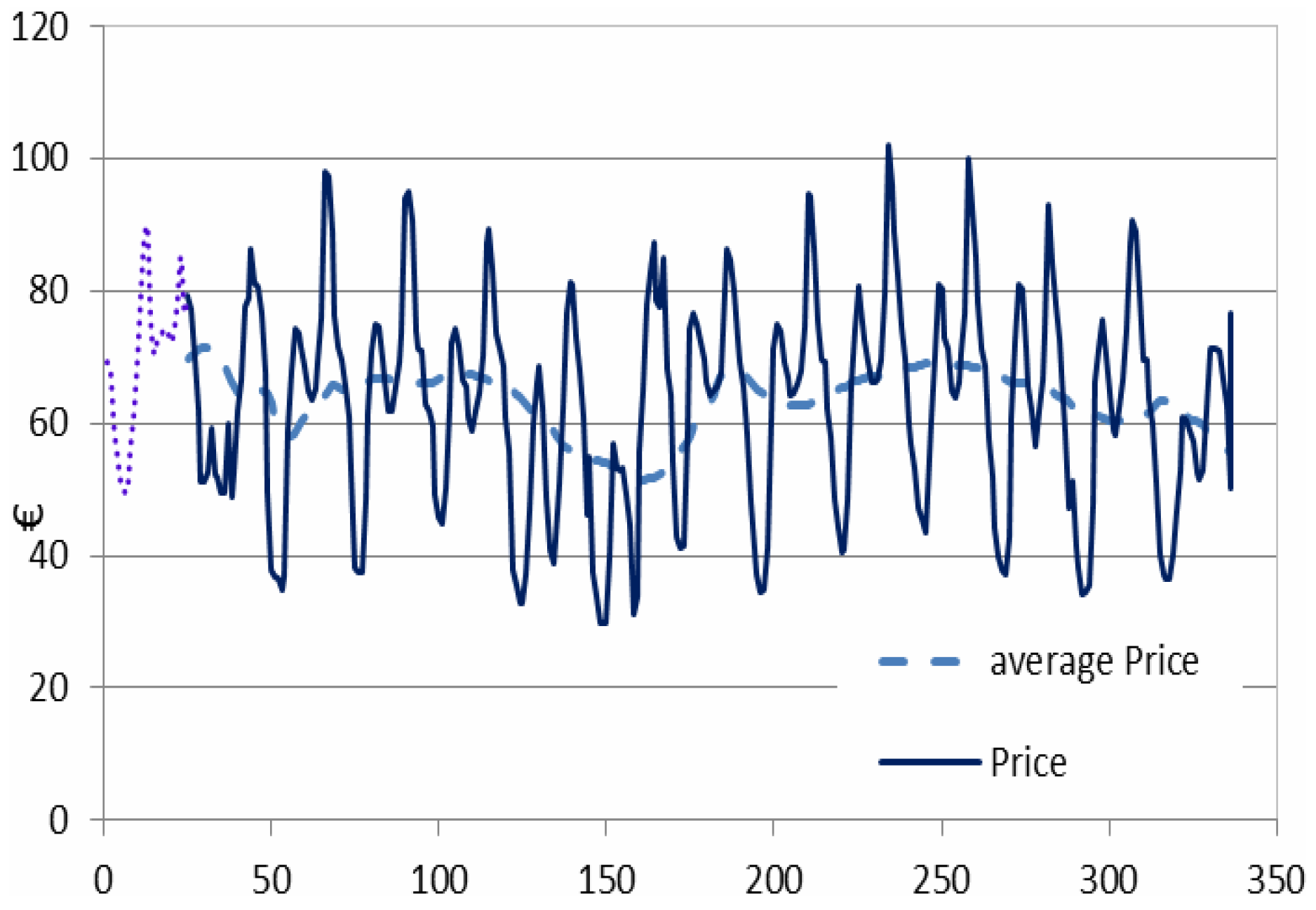
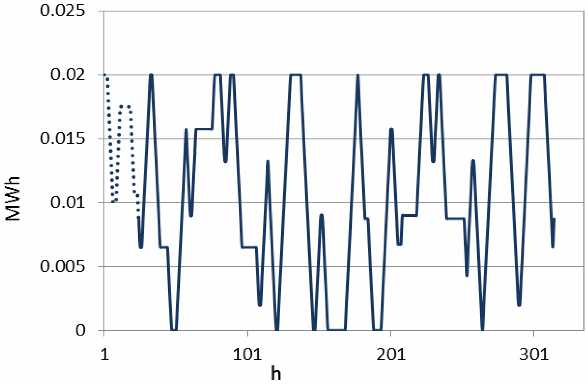
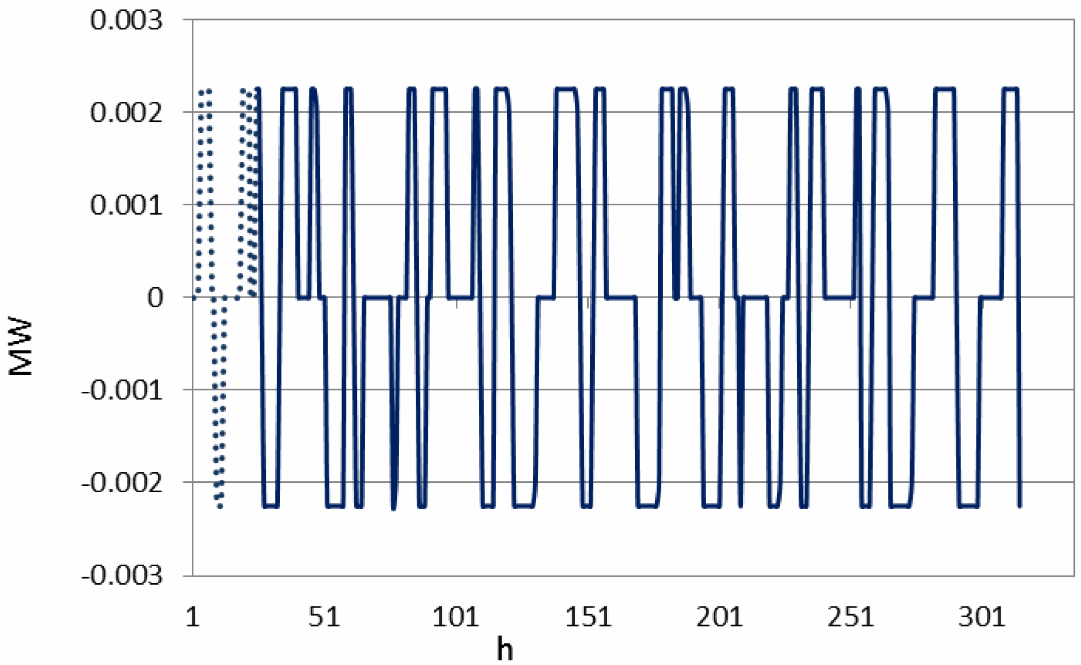
In the case of unstable behavior, the price trend is shown in Figure 15, which shows also the course of the hourly average price in the previous 24 h, used in the fuzzy rules. Figure 16 and Figure 17 respectively show the course of SOC and of the power supplied from the battery. The dotted line in Figure 15, Figure 16 and Figure 17 refers to the initial conditions.

Figure 15. Price course along 14 days—unstable scenario.

Figure 15. Price course along 14 days—unstable scenario.

Figure 16. ESS SOC course along 14 days obtained—unstable scenario.

Figure 16. ESS SOC course along 14 days obtained—unstable scenario.

Figure 17. Power supplied from the battery along 14 days—unstable scenario.

Figure 17. Power supplied from the battery along 14 days—unstable scenario.

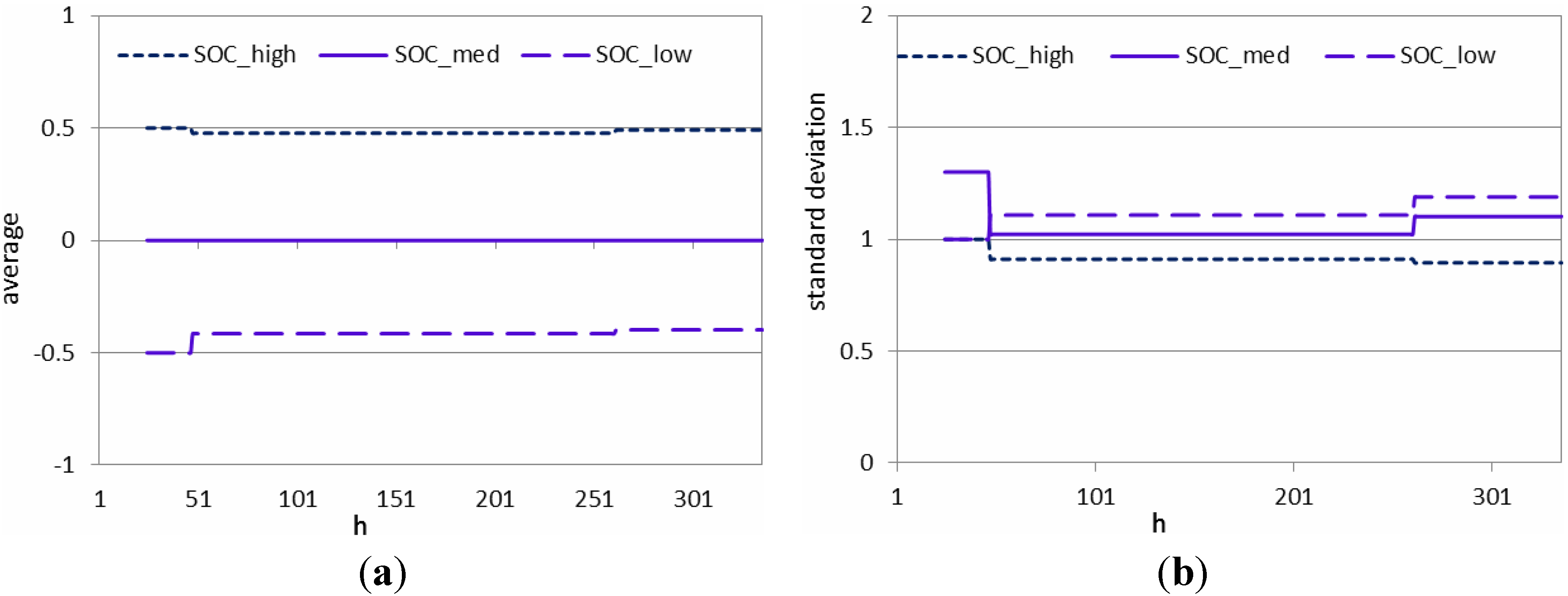
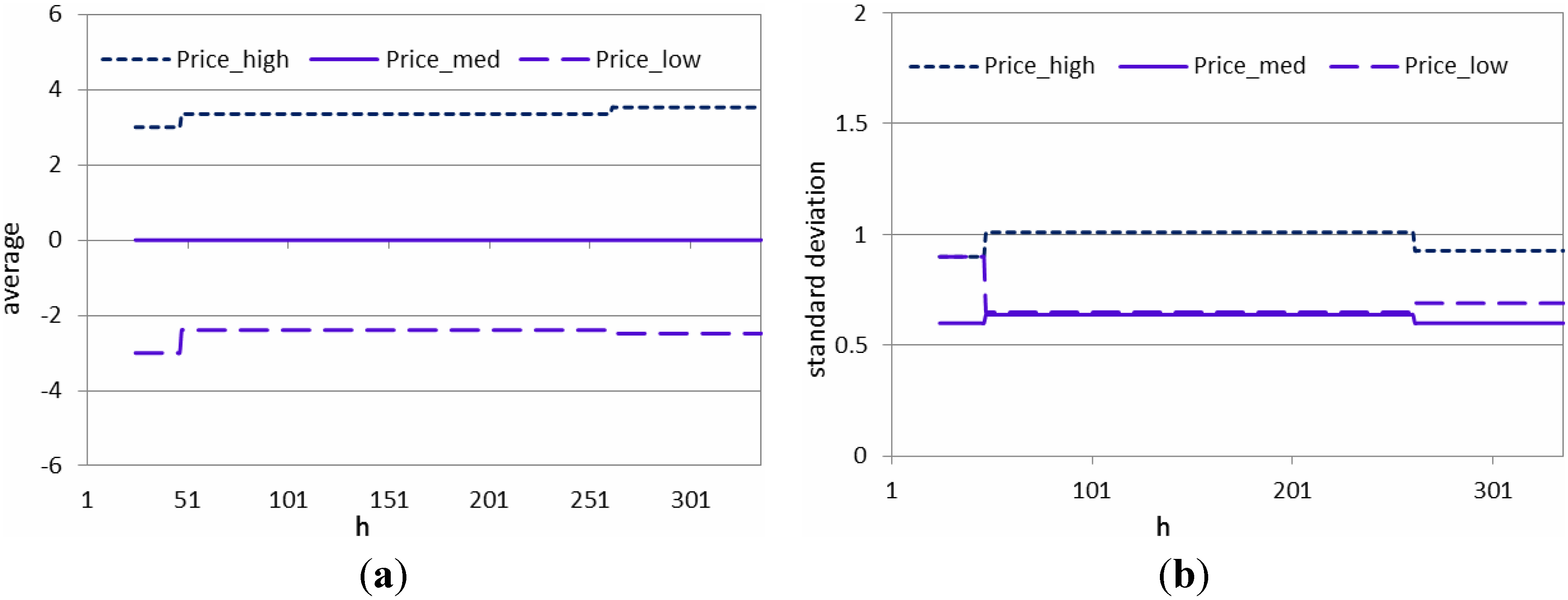
In the following figures the variations of the parameters of the MFs functions during the self-adapting process are shown. In particular, Figure 18 shows the behavior of the average parameters μ (Figure 18a) and the standard deviation parameters σ (Figure 18b) related to the Δ_SOC variable. Figure 19a,b show the behavior of the same parameters, related to Price variable. Such behavior are taken for one single run. As it can be observed comparing Figure 12 and Figure 13 with Figure 18 and Figure 19 it seems that the need for self-adaptation is less strong, as compared to the stable scenario. There are two reasons for such behavior. On one side, the initial tuning of the fuzzy controller parameters is good. Secondarily, due to the extremely variable scenario, a too strong change of such parameters would lead to a very poor economic return. Some trials have indeed been done increasing the amplitude of the random mutation above the considered 10% that have shown an undesirable behavior.

Figure 18. (a) Average parameters μ behaviour for SOC_low, SOC_med and SOC_high MFs and (b) standard deviation σ parameters courses for SOC_low, SOC_med and SOC_high MFs.

Figure 18. (a) Average parameters μ behaviour for SOC_low, SOC_med and SOC_high MFs and (b) standard deviation σ parameters courses for SOC_low, SOC_med and SOC_high MFs.

Figure 19. (a) Average parameters μ courses for Price_low, Price_med and Price_high MFs and (b) standard deviation σ parameters courses for Price_low, Price_med and Price_high MFs.

Figure 19. (a) Average parameters μ courses for Price_low, Price_med and Price_high MFs and (b) standard deviation σ parameters courses for Price_low, Price_med and Price_high MFs.

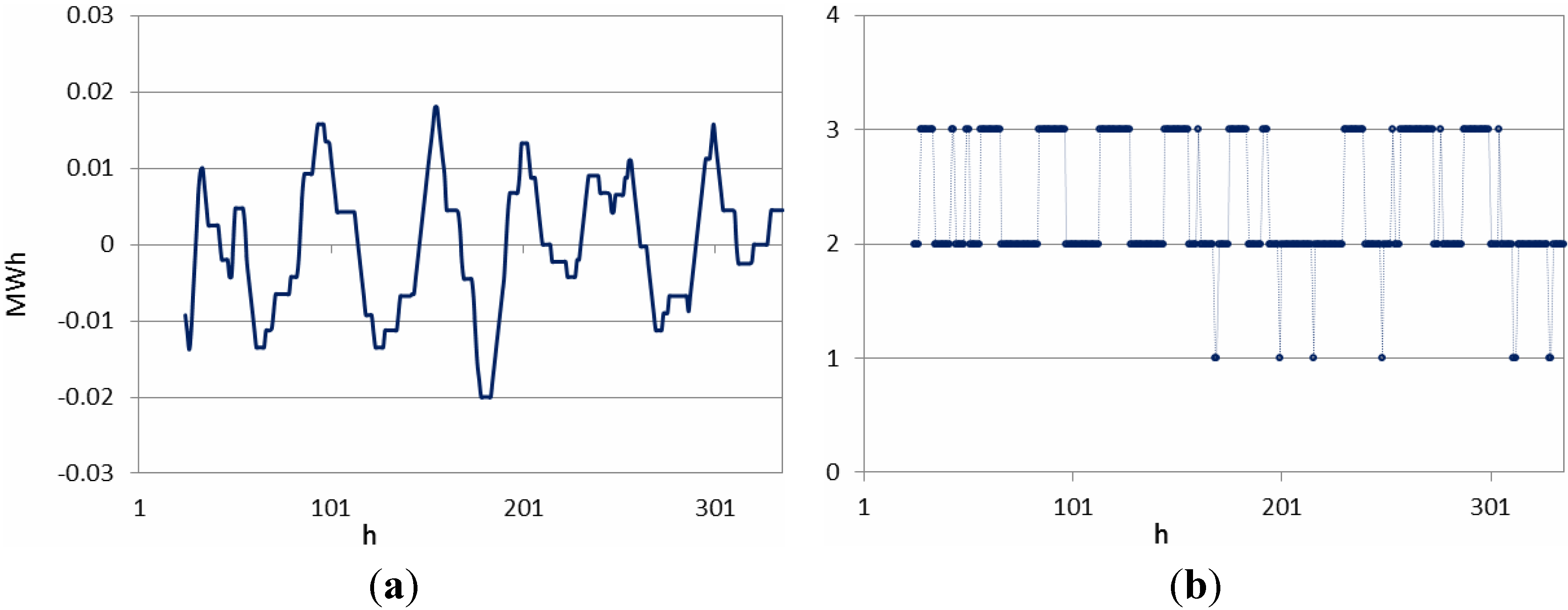
For the same unstable scenario, the following Figure 20 shows the value assumed by the technical constraints: the energy stored and released over the previous 24 h Δ_SOC (Figure 20a) and the number of maneuvers in the previous 24 h n_m (Figure 20b). Figure 20a shows that as expected, the value of Δ_SOC calculated over the previous 24 h does not tend to zero in an unstable operating condition.

Figure 20. (a) Energy stored and released, Δ_SOC, over the previous 24 h and (b) Number of operations over the battery calculated in each hour within the previous 24 h.

Figure 20. (a) Energy stored and released, Δ_SOC, over the previous 24 h and (b) Number of operations over the battery calculated in each hour within the previous 24 h.

4.3. Self-Adaptation vs. Fixed MFs Parameters

Finally, the efficiency of the self-adaptation mechanism has been tested by comparing a simulation carried out with static MFs parameters and with self-adapting MFs parameters in the two studied scenarios.

To do so, for the initial conditions above reported, a first set of runs with fixed MFs parameters (without self-adaptation) has been carried out. In Table 2, the comparison of the economic benefit obtained in a two weeks period is reported. The economic benefit has been evaluated with static analysis using Equation (7), starting from different parameter settings of the MFs.

Table 2. Economic benefit with static parameters—stable scenario.

MFs	MFs parameters	Set 1	Set 2	Set 3	Set 4	Set 5
ΔSOC	μlow	−1.3	−0.3	−0.5	−4	−0.5
	σlow	1	3	1.3	0.8	0.5
	μmed	0	0	0	0	0
	σmed	1	1.3	0.6	2	1
	μhigh	1.3	5	1.2	2	1
	σhigh	1	0.8	0.7	0.7	0.8
Price	μlow	−2	−4	−4	−2	−1
	σlow	0.9	0.6	2	1.8	1.3
	μmed	0	0	0.5	0	0.1
	σmed	0.6	0.7	0.6	0.6	0.6
	μhigh	2	4	2	2	5
	σhigh	0.9	0.6	1.4	1.8	0.9
Economic benefit (€)		5.73	3.19	4.01	5.67	3.26

Table 2. Economic benefit with static parameters—stable scenario.

MFs	MFs parameters	Set 1	Set 2	Set 3	Set 4	Set 5
ΔSOC	μlow	−1.3	−0.3	−0.5	−4	−0.5
	σlow	1	3	1.3	0.8	0.5
	μmed	0	0	0	0	0
	σmed	1	1.3	0.6	2	1
	μhigh	1.3	5	1.2	2	1
	σhigh	1	0.8	0.7	0.7	0.8
Price	μlow	−2	−4	−4	−2	−1
	σlow	0.9	0.6	2	1.8	1.3
	μmed	0	0	0.5	0	0.1
	σmed	0.6	0.7	0.6	0.6	0.6
	μhigh	2	4	2	2	5
	σhigh	0.9	0.6	1.4	1.8	0.9
Economic benefit (€)		5.73	3.19	4.01	5.67	3.26

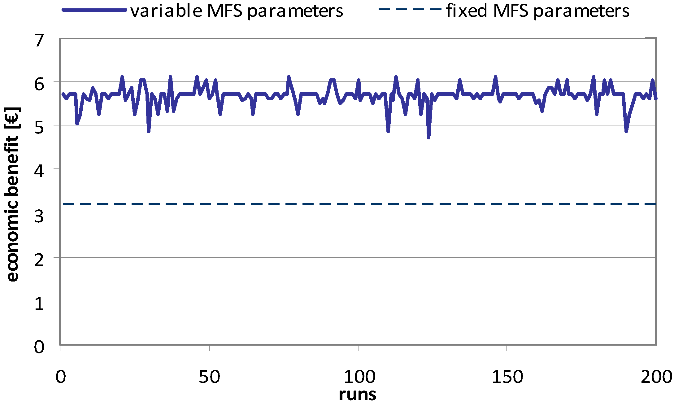
Then taking the worst set of parameters as starting parameters, a self-adaptation approach has been used. Figure 21 shows the economic benefit over 200 runs. In the figure, also the value obtained using static MFs parameters (dashed line) is reported. It is evident that in case of self-adaptation, the parameters adapt to the situation and the economic benefit results higher.

Figure 21. Comparison of the economic benefit after two weeks obtained in 200 runs for fixed and self-adapting sets of MFs parameters—stable scenario.

Figure 21. Comparison of the economic benefit after two weeks obtained in 200 runs for fixed and self-adapting sets of MFs parameters—stable scenario.

For unstable scenario, Table 3 shows the comparison of the economic benefit obtained in the two weeks with static analysis, starting from different parameter settings of MFs; the economic benefit has been evaluated using Equation (7).

Table 3. Economic benefit with static parameters—unstable scenario.

MFs	MFs parameters	Set 1	Set 2	Set 3	Set 4	Set 5
ΔSOC	μlow	−2.5	−0.5	−4.2	−0.5	−0.9
	σlow	1.5	1	1.8	0.5	0.3
	μmed	0	0	0	0	0
	σmed	1	1.3	3	1	2
	μhigh	2.5	0.5	4.2	1	0.9
	σhigh	1.5	0	1.8	0.8	0.3
Price	μlow	−1	−3	−5	−1	−0.5
	σlow	0.6	0.9	0.9	1.3	1.7
	μmed	0	0	0	0.1	0
	σmed	0.7	0.6	0.6	0.6	0.4
	μhigh	1	3	5	5	3
	σhigh	0.6	0.9	0.9	0.9	0.9
Economic benefit (€)		4.71	5.89	4.86	5.29	5.35

Table 3. Economic benefit with static parameters—unstable scenario.

MFs	MFs parameters	Set 1	Set 2	Set 3	Set 4	Set 5
ΔSOC	μlow	−2.5	−0.5	−4.2	−0.5	−0.9
	σlow	1.5	1	1.8	0.5	0.3
	μmed	0	0	0	0	0
	σmed	1	1.3	3	1	2
	μhigh	2.5	0.5	4.2	1	0.9
	σhigh	1.5	0	1.8	0.8	0.3
Price	μlow	−1	−3	−5	−1	−0.5
	σlow	0.6	0.9	0.9	1.3	1.7
	μmed	0	0	0	0.1	0
	σmed	0.7	0.6	0.6	0.6	0.4
	μhigh	1	3	5	5	3
	σhigh	0.6	0.9	0.9	0.9	0.9
Economic benefit (€)		4.71	5.89	4.86	5.29	5.35

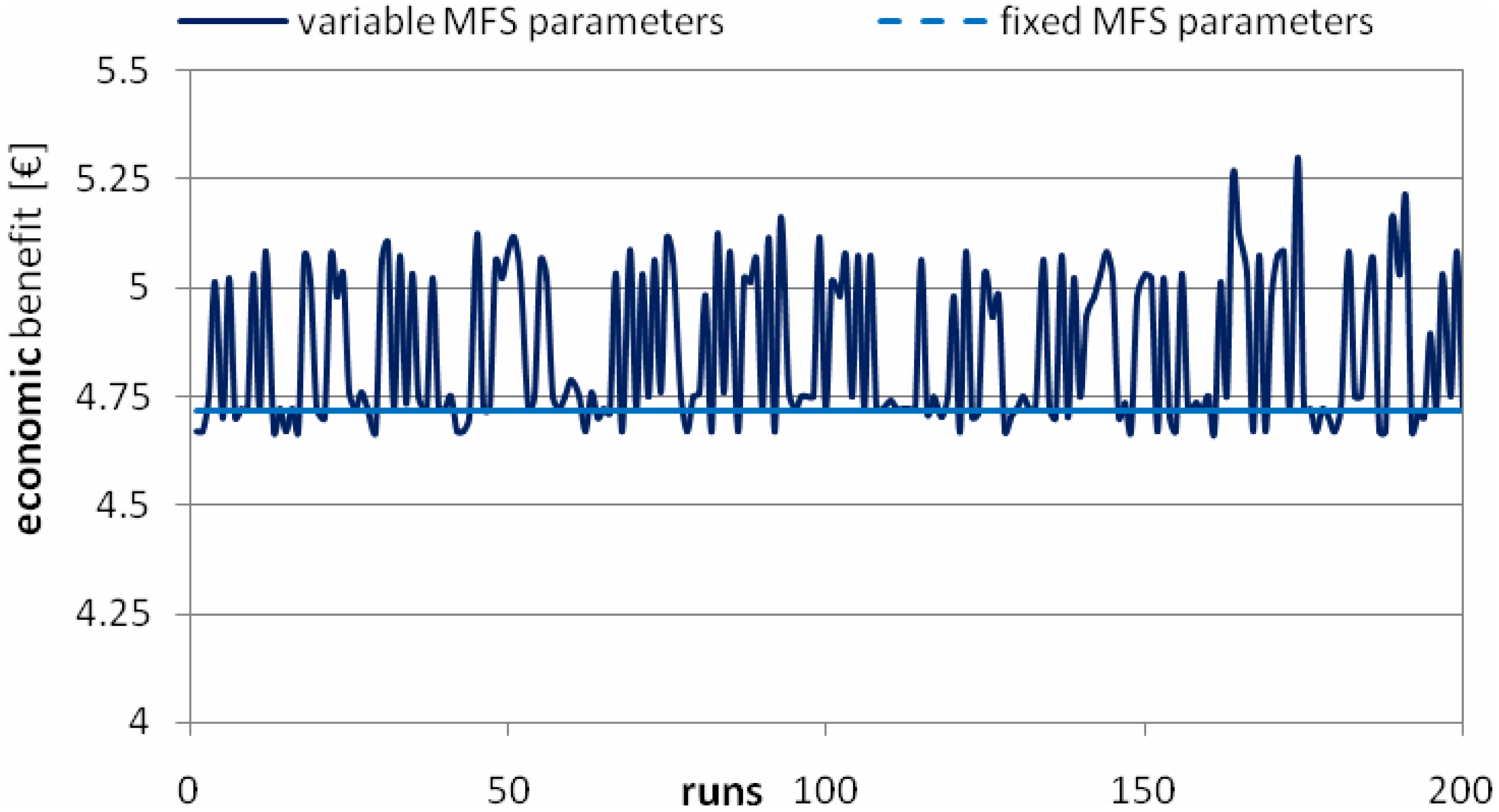
Figure 22 shows the economic benefit over 200 runs, in the case of unstable scenario, using a self-adaptation approach and taking the worst set of parameters in Table 3 as starting parameters. In the figure, also the value obtained using static MFs parameters (dashed line) is reported. It is evident that in case of self-adaptation, the parameters adapt to the situation and the economic benefit results higher.

Figure 22. Comparison of the economic benefit after two weeks obtained in 200 runs for fixed and self-adapting sets of MFs parameters—unstable scenario.

Figure 22. Comparison of the economic benefit after two weeks obtained in 200 runs for fixed and self-adapting sets of MFs parameters—unstable scenario.

5. Discussion

To emphasize the importance of the ability to adapt the parameters of the functions MSF, simulations have been performed with and without the self-adaptation mechanism. In the case of self-adaptation, the economic benefit along the two weeks has resulted always higher than in the case of static parameters values for stable scenario.

Moreover, in this latter case, different simulations with the same initial SOC, number of manoeuvres and past performance of P_batt have been carried out, giving different initial values to the parameters of the MFS.

Only the average value for the MFs_med curve of SOC membership function has been set up always to zero, without adjustments, in line with the meaning of the desired behavior of tending to the satisfaction of the bond integral battery.

The accuracy of the result has come out dependent on the starting values of the parameters. In addition, the optimal values has found to be dependent on the type of scenario represented and of the system past history: initial conditions, price change, number of operations carried out by the battery, etc.

This enhanced the choice of making variable the value of the parameters if the result obtained is not considered satisfactory. In the unstable scenario, the economical benefit is generally lower than in the stable scenario. And almost for all initial conditions, the self-adaptation mechanism improves the economic benefit.

In both scenarios, the technical constraint about the number of maneuvers is always respected as evidenced in Figure 14b and Figure 20b. The course of the SOC tends to zero in the unstable scenario but keeps oscillating values, while in the stable scenario it tends to zero as expected.

6. Conclusions

In this work, the issue of defining a suitable forecast less scheduling algorithm for ESS charge controller is studied. The problem of reducing the impact of prediction errors in scheduling is here considered and a solution approach based on a rolling horizon system that looks backwards is proposed. The system looks at the past hours to fix possible constraints violations and to improve its behaviour increasing the economic benefit, when the system is no more adequate with mutated external energy prices scenario a self-adapting mechanism adjusts the relevant parameters. The approach looks at the past experience and learns based on it.

Future work will address the following issues:

investigate different learning mechanisms;

include other rules to get different objectives;

create a real rolling horizon with self-adaptation features looking forward and backwards, weighting forecasts considering their inherent limited reliability;

extend the approach to include the possibility for the prosumer to sell energy to the grid with different energy market architectures.