Methane Gas Hydrate Stability Models on Continental Shelves in Response to Glacio-Eustatic Sea Level Variations: Examples from Canadian Oceanic Margins

Abstract

We model numerically regions of the Canadian continental shelves during successive glacio-eustatic cycles to illustrate past, current and future marine gas hydrate (GH) stability and instability. These models indicated that the marine GH resource has dynamic features and the formation age and resource volumes depend on the dynamics of the ocean-atmosphere system as it responds to both natural (glacial-interglacial) and anthropogenic (climate change) forcing. Our models focus on the interval beginning three million years ago (i.e., Late Pliocene-Holocene). They continue through the current interglacial and they are projected to its anticipated natural end. During the current interglacial the gas hydrate stability zone (GHSZ) thickness in each region responded uniquely as a function of changes in water depth and sea bottom temperature influenced by ocean currents. In general, the GHSZ in the deeper parts of the Pacific and Atlantic margins (≥1316 m) thinned primarily due to increased water bottom temperatures. The GHSZ is highly variable in the shallower settings on the same margins (~400–500 m). On the Pacific Margin shallow GH dissociated completely prior to nine thousand years ago but the effects of subsequent sea level rise reestablished a persistent, thin GHSZ. On the Atlantic Margin Scotian Shelf the warm Gulf Stream caused GHSZ to disappear completely, whereas in shallow water depths offshore Labrador the combination of the cool Labrador Current and sea level rise increased the GHSZ. If future ocean bottom temperatures remain constant, these general characteristics will persist until the current interglacial ends. If the sea bottom warms, possibly in response to global climate change, there could be a significant reduction to complete loss of GH stability, especially on the shallow parts of the continental shelf. The interglacial GH thinning rates constrain rates at which carbon can be transferred between the GH reservoir and the atmosphere-ocean system. Marine GH can destabilize much more quickly than sub-permafrost terrestrial GHs and this combined with the immense marine GH reservoir suggests that GH have the potential to affect the climate-ocean system. Our models show that GH stability reacts quickly to water column pressure effects but slowly to sea bottom temperature changes. Therefore it is likely that marine GH destabilization was rapid and progressive in response to the pressure effects of glacial eustatic sea level fall. This suggests against a catastrophic GH auto-cyclic control on glacial-interglacial climate intervals. It is computationally possible but, unfortunately in no way verifiably, to analyze the interactions and impacts that marine GHs had prior to the current interglacial because of uncertainties in temperature and pressure history constraints. Thus we have the capability, but no confidence that we can contribute currently to questions regarding the relationships among climate, glacio-eustatic sea level fluctuations and marine GH stability without improved local temperature and water column histories. We infer that the possibility for a GH control on climate or oceanic cycles is speculative, but qualitatively contrary to our model results.

1. Introduction: Marine Gas Hydrates as a Possible Mechanism of Climate and Oceanic Change

Marine methane gas hydrate (GH) dissociation (Figure 1) on continental shelves due to glacio-eustatic reduction of water column pressure is proposed as an auto-cyclic mechanism controlling climate during glacial-interglacial intervals. Marine methane GHs are proposed to have exerted a major control on past climates, both for the glacial-interglacial periods [1,2], but also for Permian and Cambrian climate-geohistory events, e.g., [3,4]. Some infer that episodic atmospheric methane flux, caused by massive to “catastrophic” marine GH destabilization driven by sea level lowering in response to the sequestering of water in continental ice sheets triggered, or is a significant cause of glacial-interglacial transitions, coined the “clathrate gun” hypothesis [2]. Recent review of the hypothesis on degassing of onshore/offshore permafrost and marine GHs [5] has concluded that “catastrophic”, widespread dissociation of methane GHs will not be triggered by continued climate warming at contemporary rates (0.2 °C per decade) over timescales of a few hundred years. That study [5] concluded that the oxidation of methane at ~50 m water depth prevents most marine methane from reaching the atmosphere. However, extensive marine methane oxidation is also a potential source oceanic anoxia. Therefore, the chemical process affecting oceanic methane events could, in the long run, cause changes in the oceanic environment.

Figure 1. Generalized scheme of marine gas hydrate (GH) stability from onshore permafrost settings to the continental slope (simplified and adapted from [5]).

Figure 1. Generalized scheme of marine gas hydrate (GH) stability from onshore permafrost settings to the continental slope (simplified and adapted from [5]).

We have adapted a model we employed previously to study GH behavior on the Quaternary continental margins of Canada accompanying glacio-eustatic cycles and their effects on sea bottom temperature and pressure variations. We also illustrate GHs preservation potential during 100 K and 41 K glacial-interglacial climate cycles. Can marine GHs survive through interglacial intervals in response to eustatic changes and sea bottom warming—like sub-permafrost GHs—where our previous work showed that GH destabilization responds to rather than causes climate changes [6]?

2. Scope

We test GH formation and dissociation models on the Canadian continental shelves during the last 14 million years (Myrs), with a focus on the last three Myrs when 41 thousand years (kyrs) and 100 kyrs glacial-interglacial cycles occurred. Our analysis emphasizes the interval since the beginning of the current interglacial since the only current control on model results is the match between current predicted and observed GH occurrences. We model three Canadian oceanic margins including:

(1)

the Pacific Ocean continental shelf offshore Vancouver Island in the region of Integrated Ocean Drilling Program Expedition 311;

(2)

the Labrador Sea continental shelf in the region affected by the Labrador Current, and;

(3)

the Atlantic Ocean continental shelf offshore Nova Scotia in the region potentially affected by the Gulf Stream.

These computer models illustrate GH stability in a variety of marine settings as a function of depth and time using temporal sea bottom temperature and pressure changes in response to both surface temperature forcing and water column pressure variations accompanying glacio-eustatic cycles.

3. Numerical Modeling Methods

We adapt the model used by Majorowicz et al. [6] and Safanda et al. [7] that employs an implicit finite-difference method similar to that described by Galushkin [8]. We have simulated time changes of subsurface temperature by solving the transient heat conduction Equation (1):

C_v ∂T/∂t = ∂[λ(∂T/∂z)]/∂z + A

(1)

where T is the temperature (K); λ is the thermal conductivity (W m⁻¹ K⁻¹); C_v is the volumetric heat capacity (J K⁻¹ m⁻³); A is the rate of heat generation per unit volume (W m⁻³); z is the depth (m); and t is the time (s) in a one-dimensional layered geothermal model of the individual sites. Equation (1) was solved numerically by an implicit finite-difference method similar to that described by Galushkin [8]. The upper boundary condition is the time-dependent surface temperature and the lower boundary condition is a constant heat flow density at 15 km. The model depth grid structure employed 2, 5, 10, 50, 100, 250 and 500 m thick elements within the depth intervals beginning at 0, 100, 1500, 2000, 2500, 5000, 10,000 and 15,000 m, respectively. The time grid steps varied from 0.5 to 50 years, depending on surface temperature changes.

The finite-difference scheme of Equation (1) on the depth and time grids ... z_k−1, z_k, z_k+1, ... and ...tⁿ, tⁿ⁺¹,..., respectively (for details see reference [6]), together with the upper and lower boundary conditions lead to a system of difference equations for unknown temperature values T_k−1ⁿ⁺¹, T_kⁿ⁺¹, T_k+1ⁿ⁺¹ (where the subscript k and the superscript (n + 1) denotes a value at the k-th depth step and the (n + 1)th time step, respectively) within a tri-diagonal matrix, which was solved by the forward method (for details see references [7,8]).

When estimating effective both the thermal conductivity values and the volumetric heat capacity we employ the geometric and arithmetic means, respectively, of the conductivity values of the rock matrix and water, matched to their volumetric proportions [8]. A contribution to the heat capacity from the latent heat of GH formation/dissociation, L (J kg⁻¹), is represented by ρΦL/(T_L − T_S), where ρ is the GH density (kg m⁻³); Φ is the total volume fraction occupied by GHs; and T_S and T_L are the temperatures of solidus and liquidus (K), respectively. Performance of the numerical code was validated by comparing its results with the analytical solution of a classical solidification problem (see reference [9] for details). We employ the free gas—GH equilibrium curve for sea water described by Equation (3); (see also Figure 4 below):

T = 8.9 × ln(depth b.s.f. + water depth) − 50.1

(2)

4. Pacific Margin Offshore Vancouver Island

The Pacific Margin continental shelf offshore Vancouver Island lies immediately to the east of a subduction zone where the Juan de Fuca and Explorer Plates are descending below the Insular Belt of the Cordilleran orogen. It is the only active subduction region on the Canadian ocean margins. Geophysical data and analysis, both bottom simulating reflections (BSR’s) and gravity, suggests that GHs occur commonly if not pervasively below the sea bottom across a huge region. These occurrences were confirmed locally by International Oceanic Drilling Project (IODP) campaigns, notably Expedition 311. This setting contrasts strongly with the Atlantic Ocean and Labrador Sea passive margins, where GH geophysical indications are few and localized in an even larger GH stability region. On the Canadian Pacific continental shelf offshore Vancouver Island we simulate GH formation and dissipation responses to changing sea floor temperature and pressure changes attending increasing sea level since the current interglacial began, ~14 kyrs ago (Figure 2).

Figure 2. Canadian Western coast GH bottom simulating reflection (BSR) occurrence zone and the location of the International Oceanic Drilling Project (IODP) Expedition 311 well.

Figure 2. Canadian Western coast GH bottom simulating reflection (BSR) occurrence zone and the location of the International Oceanic Drilling Project (IODP) Expedition 311 well.

4.1. Model Construction Pacific Margin

For these simulations of GH behavior we have adopted generally the geothermal model and sea floor temperature used by Taylor et al. [10] in area investigated by IODP Expedition 311. We have started modeling with the case of deep water with the present water depth of 1316 m and the bottom simulating reflector at the depth 225 m below sea floor (mbsf). We assume regional terrestrial heat flow of 65 mW m⁻² consistent with the Heat Flow Map of North America [11]. The lithological model we assume following Westbrook et al. [12] but simplified in three layers:

(1)

Unit I extend from 0 mbsf to 128 mbsf, with a porosity of 58%, a hydrate saturation 20%, a thermal conductivity of 1.14 W m⁻¹ K⁻¹, a specific heat capacity of rock containing a free gas of 3.51 × 10⁶ J m⁻³ K⁻¹, and rock containing GH of 3.20 × 10⁶ J m⁻³ K⁻¹;

(2)

Unit II extends between 128 m and 300 m, with a porosity of 51%, a hydrate saturation of 20%, a thermal conductivity 1.14 W m⁻¹ K⁻¹, a specific heat capacity of rock containing free gas of 3.40 × 10⁶ J m⁻³ K⁻¹ and rock containing GH of 3.12 × 10⁶ J m⁻³ K⁻¹;

(3)

Unit III extends below 300 m, with a porosity 47%, a hydrate saturation of 20%, thermal conductivity of 1.14 W m⁻¹ K⁻¹, a specific heat capacity of rock containing free gas 3.33 × 10⁶ J m⁻³ K⁻¹ and rock containing GH of 3.08 × 10⁶ J m⁻³ K⁻¹.

We assume a sea floor temperature −1.3 °C before 13.5 kyrs ago, followed by a linear increase of 4 °C to 2.7 °C occurring between 13.5 kyrs and 12.5 kyrs.

The steady-state initial temperature—depth profile below the sea floor is assumed to be in equilibrium with the sea floor temperature of −1.3 °C and a deep heat flow of 65 mW m⁻². This results in a marine GHs model between the sea floor and 283.5 mbsf at 14 kyrs ago. Depth grid steps where at 2, 5, 10, 50, 100, 250 and 500 m in the intervals from: 0–400–1,500–2,000–2,500–5,000–10,000–40,000 m. Time steps are taken at between 0.5 and 20 years depending on the rate of sea floor temperature changes and sea level variations.

The Holocene sea level rise of 120 m is modeled with two 60 m steps. Following the sea level rise record, the first occurring 14 kyrs ago and the second occurring 9 kyrs ago. The sea level rise scenario ensures that the downward shift of the GH base at each step extends over several depth grid points in the numerical simulation ensuring the proper model consideration of the latent heat release.

4.2. Model Results Pacific Margin Offshore Vancouver Island

We have calculated marine Vancouver Island GH models of for current water depths of 400, 1196, 1256 and 1316 m throughout the current interglacial −13.5–11.5 kyrs both for the constant sea bottom temperature of 2.7 °C and also for an assumed sea bottom temperature warming to 8.7 °C in the next 300 years (the assumed 6 °C future warming is based on global circulation model predictions from Intergovernmental Panel on Climate Change of 2007 [13]). The predicted GH stability base can be validated against current observed and inferred GHs. The first simulation result is for 1316 m water depth (Figure 3).

Figure 3. Modeling of GH response to the changing sea floor temperature and the increasing sea level since 14 thousand years (kyrs) ago on the continental shelf, offshore Vancouver Island.

Figure 3. Modeling of GH response to the changing sea floor temperature and the increasing sea level since 14 thousand years (kyrs) ago on the continental shelf, offshore Vancouver Island.

Model results (Figure 3) illustrate both key model input parameters, such as sea bottom temperature (°C) and water depth (m). The key computed result is the gas hydrate base, and sometimes the GH top and its variation with depth below sea floor with time. The inferred BSR depth, ~225 mbsf, in 1316 m of water is shown for comparison. Taylor [10] states that the observed GH base occurs 30–35 m below the inferred depth of the BSR at ~260 mbsf, which is close to the current model prediction of 255.3 mbsf (Figure 3). The GH stability top is not shown, as it occurs within the water column. While GH found on the sea floor discontinuously, GHs are rare in the water column due to oceanic under saturation with respect to methane, in part due to methane oxidation [5].

Sea floor warming effects are more important and protracted than pressure effects attending sea level rise. Comparison of the model result (Figure 3) to the equilibrium GH phase stability curve as a function of water depth and its intersection with the geothermal profile (Figure 4). At the end of the last glacial the model is in equilibrium with the 1196 m water column during the sea level low-stand. The current model GH base (Figure 3) is at 255.3 mbsf this is approaching equilibrium (Figure 4) for its current water depth. The model suggests that it takes ~14 kyrs to approach thermal equilibrium for a sea bottom temperature increase of 4 °C accompanied by 120 m sea level rise. This illustrates how GHs respond and dampen the effects of climate and oceanographic changes rather than driving them, irrespective of the fate of methane released into the water column [5]. The damped and muted GH response (Figure 3) suggests there is nothing “explosive” or sudden about the clathrate gun.

Figure 4. Temperature depth and hydrate phase curve for water depth 1196–1316m for the marine hydrate Vancouver Island case of postglacial warming and related sea bottom warming.

Figure 4. Temperature depth and hydrate phase curve for water depth 1196–1316m for the marine hydrate Vancouver Island case of postglacial warming and related sea bottom warming.

Our GH destabilization rates are about 6% lower than those reported previously [10]. Taylor [10] considered water depths 400, 500, 800, 1300 and >1800 m and calculated that the time for the dissociation of 30 m of model GH was 2 kyrs in 500 m water depth and 10 kyrs in 1800 m water depth. Our result (Figure 4) can be compared against their result (their Figure 5a and Figure 9). They suggest that the 30 m GH layer at the base of GHs dissipates completely in 8.5 kyrs when water depth is 1300 m [10]. However, our models show that the consideration of GH latent heat effects accompanying sea level rise slows GH destabilization. Thus in our models the GH thickness at the end of the last glacial, 13.5 kyrs, 283.5 m, thins to 255.3 m currently, which is 28.2 m, or 6% less than that suggested by the models of others [10]. The current 30 m thick GH layer is predicted to dissociate completely within a few thousand years into the future.

The shallow Pacific Margin model, ~400 m water column, exhibits a completely different result (Figure 5). It predicts that GHs dissociated completely within about two millennia following the last glacial. This is due to the combination of shallow water and increased sea bottom temperature, where GHs are not stable in the water column and as a result they dissociated from both the top and base of the GH layer. However, GHs become stable again, at this location, subsequent to the second eustatic sea level rise 9 kyrs ago, due to the increased water column pressure regardless of the eustatic model. After 9 kyrs ago the GHs grow downward quickly to ~20 mbsf within about 1.5 kyrs ago. Subsequently and until the present, the reformed GH layer thins only slightly as the transient effects of the second sea level increase decrease and the thermal effects of both sea bottom temperature and latent heat are re-established. Therefore we predict that Pacific Margin GHs in water depths less than ~400 m have a younger formation age and a different history from those underlying the deeper Pacific Margin continental shelf. Projected to the end of the current interglacial the thickness of these GHs changes little. On the shallow Pacific Margin the changes in GH history are rapid and marked, in contrast to the deeper setting, where they change slowly during the interglacial. However, the thickness of the gas hydrate stability zone (GHSZ) on the shallow continental shelf is less than one third that in the deeper settings. Therefore, although the results are dramatic, the magnitude of the effect is subordinate.

Figure 5. Marine GH model for the Vancouver Island offshore for 400 m present water depths for the interglacial −13.5–11.5 kyrs both for the constant sea bottom 2.7 °C temperature and for a warming to 8.7 °C in the next 300 years.

Figure 5. Marine GH model for the Vancouver Island offshore for 400 m present water depths for the interglacial −13.5–11.5 kyrs both for the constant sea bottom 2.7 °C temperature and for a warming to 8.7 °C in the next 300 years.

4.3 Future Pacific Margin GHs and Climate-Ocean Changes

The future behavior of the deeper Pacific marine GH model depends primarily on the sea floor temperature (Figure 5 and Figure 6). If we assume that sea bottom temperatures remain constant (2.7 °C in 1316 m water depth, Figure 6), as they have been since 12.5 kyrs then the equilibrium GH layer thickness will be 220 m in a water depth of 1316 m at the expected end of the current interglacial. This is only slightly shallower than its present depth of 255.3 m. We use this example to predict roughly the future volumes of methane available to be released into the water column. We assume that the methane volume liberated from destabilized GHs represents a maximum estimate of the methane volume that might be introduced into the ocean-atmosphere systems, while we recognized that biological and chemical processes might detain some of this methane below the sediment-water interface.

Figure 6. Simulated future GH base assuming a 6 °C sea bottom warming. The equilibrium GH layer base for temperatures of 2.7 °C and 8.7 °C are 219 m and 101 m, respectively. The model GH bases are much deeper, 243.7 m and 163.3 m, respectively, at the end of the interglacial due to effects discussed in the text.

Figure 6. Simulated future GH base assuming a 6 °C sea bottom warming. The equilibrium GH layer base for temperatures of 2.7 °C and 8.7 °C are 219 m and 101 m, respectively. The model GH bases are much deeper, 243.7 m and 163.3 m, respectively, at the end of the interglacial due to effects discussed in the text.

A current water column like that used in our first, deeper, model (Figure 3) corresponds to the model shown in Taylor et al.’s [10] Figure 2. We have extended the simulation for 1316 m water depth to the “anticipated” end of the current interglacial (Figure 6). If we assume, in accord with our previous interglacial duration of 25 kyrs and our assumption of its onset ~13.5 kyrs ago, the current interglacial ends 11.5 kyrs in the future. We have considered two scenarios for this future prediction. The first is a constant sea bottom temperature, 2.7 °C. The second future scenario considers a 6 °C increase in 300 years (similar to global ground surface temperature changes in previous models). We are aware that even if the air warms during the next 300 years by 6 °C that the sea bottom warming will be probably be smaller, but we use 6 K as an upper estimate of the possible change. The equilibrium depths for the GH base when future sea bottom temperatures are, respectively, 2.7 °C and 8.7 °C are 219 m and 101 m, but as one can see from Figure 6, the model GH bases are much deeper at the end of the current interglacial, at 243.7 m and 163.3 m, respectively when the full effects of sea level rise and enthalpies are considered (Figure 6). We calculated effectively the same model reported by Taylor [10] in order to compare the time for a 30-m GH layer to decay (not considering sea level rise in this case). For a 1300 m water depth our simulation indicates that a 30-m GH layer dissipates completely 8440 years after the beginning of interglacial warming, which agrees with Taylor et al.’s [10] estimate of 8.5 kyrs to produce the same effect, when the impact of sea level change is neglected.

The annual methane release rate from the destabilizing GH can be calculated following the model GH change rate (Figure 6). We have considered 51% porosity, 20% saturation, density of hydrate 910 kg m⁻³ and weight ratio of Type I methane hydrate equal to 0.134. Figure 7 depicts the annual model methane release rate history (Figure 6, in grams per square meter per year). The small rate oscillations are an artifact of the simulation. The large rate singularities , are artifacts of the sea level rise model employed accompanying the instantaneous GH base drop during the sea level rises at 14 kyrs and 9 kyrs ago. These later singular artifacts are much larger than shown, but they are truncated for purposes clarity.

Figure 7. The annual methane release rate (g m⁻² yr⁻¹) for the GH history scenario in Figure 6.

Figure 7. The annual methane release rate (g m⁻² yr⁻¹) for the GH history scenario in Figure 6.

One result, for the shallowest marine GHs in 400 m of water, is shown in Figure 5. The model suggests that GH destabilize completely following the initial warming begins 14 kyrs, but that GHs begin to form and expand downwards following the second interval of sea level rise 9 kyrs. Whether GH persists to the end of the current interglacial is shown to depend entirely on bottom water temperatures in the future. Although the model and the water depth is the same as that considered previously (Figure 4 in reference [10]), the results are different, primarily because our original hydrate thickness at time 13.5 kyrs ago is not 30 m, but 49 m as a result of the different models used. These differences include the slightly different hydrate p-T curve used previously [10], which considered a constant hydrate equilibrium temperature 0.5 °C between the sea floor and the 30 m depth, whereas our phase boundary equation yields 0.955 °C for 30 m depth and gives an original GH thickness of 49 m in our models. The two models also differ on the time required for complete dissociation. Our models suggest 1920 years since warming began compared to 700 years [10]. The difference results from both original thicker GH of our model and the lesser pressure effect of a 60 m sea level rise beginning −14 kyrs.

After the second increment of sea level rise 9 kyrs ago (Figure 5, new GH begins to form again and it reaches currently to a depth of about 20 m. If a constant sea floor temperature 2.7 °C persists then the neo-formed GH layer survives until the end of the interglacial 11.5 kyrs in the future when it is 17 m thick. Equilibrium models for the end of the current interglacial would suggest a 15 m GH layer. If, instead, the sea bottom temperature increased as modeled above, then the neo-formed GH layer that grew since the second stepwise increase in sea level disappears shortly after the future warming of the sea floor begins.

5. Labrador Margin

We also model GH stability under changing bottom water temperature and water column conditions for the Atlantic margin. The Atlantic passive margin is divided into a number of segments controlled by local tectonic history accompanying the generally northward propagation of the Atlantic Ocean during the Mesozoic and Tertiary, including its abandoned foray between Canada and western Greenland. As a result, the continental shelf on the Atlantic and Labrador margin varies in width from about 100 km offshore Labrador to more than 600 km off Newfoundland (Figure 8). Parts of the Grand Banks are less than 50 m deep, while some troughs are 400 m deep. Beyond the shelf edge, the ocean floor descends to >2000 m. Despite the significant depth variations the sea bottom temperatures vary little due to the strong influence of currents.

Figure 8. Atlantic Margin shelf water depths.

Figure 8. Atlantic Margin shelf water depths.

Figures 9. Predicted GH thickness for (a) offshore Labrador and (b) the Grand Banks region modified here from predicted previously [14].

Figures 9. Predicted GH thickness for (a) offshore Labrador and (b) the Grand Banks region modified here from predicted previously [14].

Majorowicz and Osadetz [14] described current GH stability on Labrador and Grand Banks margin (Figure 9). They noticed that GH stability zone thickness increases rapidly from 330 m to ~400 m where the water column is <1 km while it increases more slowly, from 400 m to 550 m, where water column varies between 1 km and 2 km, indicating that the pressure effect due to water column is greatest where the water column is <1000 m. Despite the broad region and immense volume of the resulting current GH stability zone [14], there are relative few, primarily geophysical, indications for GHs, specifically BSR’s, which suggests other petroleum system controls control GHs on this margin, limiting them to a few localities [15].

The Labrador Current (Figure 10) exerts a significant cooling effect on the sea floor of the Labrador Shelf. Compared to the main body of the North Atlantic Ocean, the Labrador Current is colder and less saline. Its thermal effects are enhanced by its strong southward flow, ~35 km a day, and its lower salinity, such that it tends to freeze more easily. By the end of an average winter coastal Labrador inlets and the inter-island waterways of the eastern Arctic Archipelago are generally frozen. Beyond the land-fast ice, Arctic and sub-Arctic ice floes are carried by the Labrador current as far south as the Grand Banks. During the spring and summer the ice pack retreats northward and by the end of July coastal waters are normally ice-free.

Figure 10. Sea currents effecting sea bottom temperatures offshore Labrador.

Figure 10. Sea currents effecting sea bottom temperatures offshore Labrador.

Ocean bottom temperature across the Labrador continental shelf is persistently cold. On an annual basis its water temperatures are 7–10 °C lower than those at corresponding latitudes on the western margins of both North America and Europe, due primarily to oceanic currents. The Labrador current flows southward at ~35 km a day. Similarly water issuing from Baffin and Hudson bays, Foxe Basin and West Greenland Current, is colder (0 °C) and less saline (0.0334 kg L⁻¹) than water of the deep ocean (4.0 °C, 0.0347 kg L⁻¹). Labrador margin sea bottom temperatures are everywhere near 0 °C currently and they are and little changed throughout the Quaternary. Sea bottom temperature changes are very small, ranging from between −2 °C and −1 °C to between 0 °C and 1 °C in the shallow ocean and remaining close to −2 °C on the deeper continental shelf. Similar ocean bottom temperatures characterize both interglacial and glacial intervals.

5.1. Labrador Margin Inferred GH Occurrences

Mosher (his Table 1 and Table 12 in reference [15]) identified three potential GH occurrences on the Labrador margin using BSR’s: (1) Makkovik Slope; (2) Hamilton Spur; and (3) Orphan Spur. The Makkovik: BSR occurs on the central Labrador Slope, off Makkovik Bank as a sporadic phase reversed BSR at 508 ms below seafloor on a number of multichannel seismic reflection profiles, in water depth between 620 m and 2555 m. In the same region ocean bottom seismometers (OBS) indicate anomalously high velocities in the top 500 ms sub-seafloor. This suggests that the BSR occurs, on average, 443 m below the sea floor and between 1336 m and 3251 m below sea level. The Hamilton Spur is a large drift deposit off the southern Labrador margin. There Mosher [15] recognized a “continuous” BSR on industrial multichannel seismic reflection profiles. It occurs, on average 440 ms below the seafloor in water depths between 1075 m and 2100 m. Orphan Spur is another thick sediment drift deposit off northern Newfoundland. It exhibits a poorly defined BSR on high resolution seismic data ~332 ms sub-seafloor where water depths are between 735 m and 1064 m, suggesting the BSR occurs about 251 m below seafloor and between 985 m and 1348 m below sea level.

5.2. Model Construction Labrador Margin

Unlike the Pacific Margin, where there appears to be a pervasive BSR there are few geophysical indications for GHs on the Labrador Margin to constrain our models. As a result our current model predictions are not as well constrained as they were for the Pacific Margin. As mentioned above the sea bottom temperature is inferred to have remained effectively constant little in this region throughout the Quaternary. Currently the sea bottom temperature is ~0 °C and the inferred total range of sea bottom temperatures for the Labrador shelf is between −2 °C and at most 1 °C, regardless either water depth or time during the glacial-interglacial cycles. The deeper heat flow is not well established. The North American Heat Flow Map [11] indicates values of 50–60 mW m⁻² and 60–64 mW m⁻² for shallower and deeper shelf, respectively. The only geothermal information available is a temperature gradient of 32 °C km⁻¹ [14], which indicates an average heat flow between 36 mW m⁻² and 64 mW m⁻² if average thermal conductivities are between 1.14 W m⁻¹ K⁻¹ and 2.00 W m⁻¹ K⁻¹, respectively.

We calculated Labrador Margin GH histories for current water depths of 500 m and 1800 m, using a thermal conductivity of 1.14 W m⁻¹ K⁻¹), a porosity between 47% and 58%, and a GH saturation of 20%. Like the Pacific Margin models we consider two step-wise sea level rises, equal to 60 m at both 14 kyrs and 9 kyrs before the present. We employed an increase of the sea bottom temperature from −2 °C to 0 °C between −13.5 kyrs and −12.5 kyrs where current water depth is 500 m and used a higher interglacial bottom water temperature, 4 °C, where the water depth is 1800 m. The simulations were projected into the future for cases accompanied by two bottom temperature scenarios, one assuming a constant future temperature and another assuming warming by 6 °C for 300 years hence as discussed above. All models assume a natural end of interglacial at 11.5 kyrs in the future.

5.3. Model Results Labrador Margin

The Labrador Sea model results are illustrated by Figure 11, Figure 12, Figure 13 and Figure 14. Figure 11 and Figure 12 illustrate key model inputs (sea bottom temperature, water depth) and GH base results for the shallower setting (currently 500 m; Figure 11) and the deeper continental shelf (currently 1800 m; Figure 12) from 14 kyrs before present to the anticipated end of the interglacial 11.5 kyrs into the future. In the shallower setting models for a constant near zero degree sea bottom temperature (turquoise) show that the base of the GH layer grew downward to a maximum depth of ~350 mbsf sea flow or ~850 below the sea level in response to the pressure effect of sea level rises. Again note the model singularities explained above. The models also show that the future GH base depends strongly on the future sea bottom temperature history. If sea bottom temperatures remain constant (turquoise) the base of the gas hydrate layer rises only slightly and it remains at >330 m below the sea floor until the onset of the next glacial interval. If, instead, the sea bottom warms significantly (blue), in response to global climate change, the base of the GH layer responds with a slight delay, to increasing sea floor temperature and GH base is <250 m below the sea floor at the end of the current interglacial, a difference of nearly 100 m or 28% thinner than the current GH layer.

Figure 11. Labrador Sea GH history models for current a 500 m water depth.

Figure 11. Labrador Sea GH history models for current a 500 m water depth.

Figure 12 illustrates four different sea bottom temperature scenarios in 1800 m current water depth. All four scenarios assume in a −2 °C sea bottom temperature at the end of the last previous glacial. Subsequently we modeled two lower temperature options, one where the sea bottom stays a constant 0 °C during the entire interglacial interval (orange) and a second where preceding interglacial sea bottom temperatures were 0 °C, but where global climate changes results in a 6 °C sea bottom temperature increase to 4 °C for 300 years in the future (purple). The warmer two models are based on a current 4 °C, outer continental shelf interglacial sea bottom temperature that remains either constant (turquoise) to the end of the current interglacial, or which exhibits a 6 °C temperature increase 300 years into the future (blue), due to global climate change.

Figure 12. Labrador Sea GH history models for current a 1800 m water depth.

Figure 12. Labrador Sea GH history models for current a 1800 m water depth.

5.4 Future Labrador Margin GHs and Climate-Ocean Changes

Figure 13 and Figure 14 illustrate the potential annual rate of methane release (kg m⁻² yr⁻¹) for models illustrated in Figure 11 and Figure 12, respectively, based on a model with 51% porosity, 20% GH saturation, using a GH density of 910 kg m⁻³ and Type I GH weight ratio of 0.134. In the shallow setting (500 m current water depth) both models indicate a significant GH thickness increase in response to sea level rises followed by a progressive thinning and methane release as thermal effects predominate during the ~4.5 kyrs that follows each sea level rise. Where the future sea bottom temperature remains constant the future annual methane liberated is essentially unchanged from the current values. However, in the case where future sea bottom temperatures warm significantly the methane release rate increase sharply to more than five times the current rate abruptly 300 years into the future, and it remain similarly high until the current interglacial ends.

On the outer continental shelf (current water depth 1800 m) the methane release rates for constant sea bottom temperature histories are either substantially lower or comparable, to methane release rates for the shallow constant sea bottom temperature model, but they are generally not much greater than 0.025 kg m⁻² yr⁻¹. Methane release rates are lower where sea bottom temperatures are 0 °C and they are comparable where sea bottom temperatures are 4 °C. The two cases that consider an increase in sea bottom temperature 300 years in the future give predictably higher rates compared to their matching constant sea bottom temperatures models, but the total rates of methane liberation is significantly lower than those of similar models in shallow settings, due to the water column pressure effects on the outer continental shelf.

Figure 13. Model methane release rate (kg m⁻² yr⁻¹) history for the Labrador Sea for a current 500 m water depth.

Figure 13. Model methane release rate (kg m⁻² yr⁻¹) history for the Labrador Sea for a current 500 m water depth.

In general, both GH stability zone history and the potential methane release rate depend on both sea bottom temperature and water column pressure effects. Sea bottom temperatures are the critical factor affecting both GH stability and methane release rate. Our models suggest that future methane release rates and their effects will be greatest where global change results in a sea bottom warming. Although the role of water column pressure is secondary to that of sea bottom temperatures the effects of both post-glacial eustatic sea level rises and the water depth profile across the continental shelf have discernable effects that increase GH thickness and reduce the methane flux as water column pressure increases, whatever the cause.

Figure 14. Model methane release rate (kg m⁻² yr⁻¹) history for the Labrador Sea for a current 1800 m water depth.

Figure 14. Model methane release rate (kg m⁻² yr⁻¹) history for the Labrador Sea for a current 1800 m water depth.

6. Atlantic Margin Continental Shelf Offshore Nova Scotia

Sea bottom temperatures are warmer on the Nova Scotia shelf than on the Labrador Margin. The difference is due primarily to differences between the effects of the cold Labrador Current and the warm Gulf Stream or Atlantic Current on sea bottom temperatures, but there are also differences in position (latitude) and sea ice conditions (Figure 8). As a result the formation and preservation of previously accumulated GH is uncommon offshore Nova Scotia, especially on the shallower continental shelf (<500 m water column).

6.1. Inferred GH Occurrences on the Atlantic Margin Offshore Nova Scotia

The predicted GH stability region offshore Nova Scotia is restricted to the outermost continental shelf and slope where elevated water column pressure effects compensate for warmer sea bottom temperatures [14]. The current equilibrium base of the gas hydrate stability zone ranges between zero, over most of the continental shelf, but it increases to up to 600 m on the outermost continental shelf and slope (Figure 15). Only a few wells indicate the potential for GH formation west of the Laurentian Channel (Figure 15). Geophysical data suggest that GHs are localized and limited in comparison to the region of GH stability, like the Labrador Margin, but unlike the Pacific Margin. Mosher [15] identified three regions, two of which lie west of the Laurentian Channel where BSR’s suggest the presence of GHs. These included: the Barrington region, were BSR’s occur over a region of 830 km², between 500 ms and 600 ms in between 2280 m and 2890 m water depth; the Mohican Channel, where <25 km² is underlain by BSR’s occurring between 400 ms and 450 ms, with a secondary BSR at ~500 ms where water depths are between 500 m and 1930 m; and the Haddock Channel BSR, which lies on the eastern flank of the Laurentian Channel, on the St. Pierre Slope in water depths between 1700 m and 2150 m where a BSR is identified between 450 ms and 500 ms.

Figure 15. Predicted Atlantic Margin GH thickness offshore Nova Scotia (modified from [14]).

Figure 15. Predicted Atlantic Margin GH thickness offshore Nova Scotia (modified from [14]).

6.2. Model Construction—Atlantic Margin

The Atlantic Margin offshore Nova Scotia has a heat flow of 60 mW m⁻². We employ a linear sea bottom temperature increase from −2 °C to 10 °C beginning 14 kyrs for an interval of 10 kyrs. Like previous models we employ a similar dual step-wise increase in water depth during the Holocene. We consider two alternatives current water depth settings between 500 m and 1800 m, representative of the inner and outermost continental shelves, respectively.

6.3. Model Results Atlantic Margin Offshore Nova Scotia

The model results are illustrated for 500 m current water depth (Figure 16) and 1800 m water depth (Figure 17). In the inner continental shelf GH history is controlled by changes in temperature and the effects of water depth and pressure variations are not significant. The relatively thick GH layer that extended to slightly more than 150 m below the sea bottom at the end of the last glacial interval begins to rise/dissociate from its base shortly after the initial increase in water column and bottom temperature beginning 14 kyrs ago (time zero, turquoise line Figure 16) The dissociation rate increases slightly after the transient pressure effects of the second step of sea level rise occurs 9 kyrs ago but subsequently the dissociation rate increases much more as the thermal effects predominate, particularly as the upper GH stability boundary impinges on the sea bottom, approximately 6.5 kyrs after the end of the last glacial (black line on Figure 16), which contributes to the accelerated rate of GH dissociation, until GHs are no longer stable anywhere in water depths currently <500 m after about 5 kyrs ago (time 9 kyrs on Figure 16).

Figure 16. Atlantic Margin marine GH history models for current a 380–500 m water depth.

Figure 16. Atlantic Margin marine GH history models for current a 380–500 m water depth.

In deeper water, 1800 m, on the outmost continental shelf the GH base reached slightly more than 375 m below the sea floor at the end of the last glacial (Figure 17). Like the shallower Scotian Shelf the GH responses to changes in water column and sea bottom temperature after 14 kyrs ago (time zero on Figure 17) are dominated by temperature changes propagating downward from the sea floor, but the effects are smaller and muted compared to the shallow model. Like the shallower model the GH base thins slowly prior to the second sea level rise at 9 kyrs after the first. GH dissociation increases significantly although most of the rise in the GH base occurs during the last 7 kyrs prior to the Present (14 kyrs on Figure 17). Currently the model GH base occurs slightly more than 300 mbsf in 1800 m water depth. The model Present GH base, ~300 mbsf, is significantly deeper than the current equilibrium GHSZ base for 1800 m water depth and a temperature of 10 °C. The current equilibrium model predicts a GH layer base at ~130 mbsf below the sea floor. Thus, the model result suggests that a relict GH layer from the end of the last glacial persists at a depth below the sea flow approximately twice that expected for newly formed gas hydrates. Therefore, it might be possible to differentiate currently formed GHs from relict GH layers formed during the last glacial.

Figure 17. Atlantic Margin marine GH history models for current a 1680–1800 m water depth.

Figure 17. Atlantic Margin marine GH history models for current a 1680–1800 m water depth.

Mosher suggests the observed BSR’s on the Scotian Shelf occurred in the two-way travel time interval between 500–600 ms (Barrington), 400–450 ms (Mohican Channel) and 450–500 ms (Haddock Channel), where water columns were 2280–2890 m, 500–1930 m and 1700–2150 m, respectively [15]. A more detailed analysis of reflection and OBS data from Mohican Channel [15] inferred a high to low velocity transition at 310–330 mbsf, which is inferred to be both locally and regionally consistent with our model predictions since the GH phase boundary is not strongly sensitive over the observed depth range at a constant temperature, as demonstrated by the arrival time similarities among the three BSR localities. A general similarity of the Atlantic margin BSR depths with our models predictions suggests that the Barrington, Mohican Channel and Haddock Channel potential GH accumulations are probably relict from the last glacial.

6.4. Past and Future Atlantic Margin GH Response to Climate-Ocean Changes

Figure 17 also illustrates the future Scotian Shelf GHs project from the Present (14 kyrs on Figure 17) to the anticipated “natural” end of the current interglacial (25 kyrs on Figure 17). The comparable interval is not illustrated for the shallow Scotian shelf model where GH dissociated completely previously. The outer Scotian Shelf model predicts the GH base continues to rise in the future at a rate comparable to that inferred currently, until it is about 225 mbsf at the end of the interglacial. Figure 18 and Figure 19 illustrate the rate of methane release. The two singularities attending the sea level rises should be ignored as discussed above.

The shallow shelf model (Figure 18) indicates that sea bottom temperature increase is the primary control on methane release rate on the Scotian Shelf.

Figure 18. Model methane release rate (kg m⁻² yr⁻¹) history for the Atlantic Margin offshore for a current 380–500 m water depth. The sharp oscillations are an artifact caused by linear interpolation of temperature between the nodes of the depth grid during the numerical differentiation.

Figure 18. Model methane release rate (kg m⁻² yr⁻¹) history for the Atlantic Margin offshore for a current 380–500 m water depth. The sharp oscillations are an artifact caused by linear interpolation of temperature between the nodes of the depth grid during the numerical differentiation.

The increase in pressure attending sea level rise does reduce methane flux, but it is a minor effect, not apparent after 1.5 kyrs, compared to temperature effects. Prior to ~7 kyrs ago, the GH is dissociating at its base only, at 1.5 kyrs after the first sea level rise, but the rate increases to ~0.19 kg m⁻² yr⁻¹ prior to the second eustatic sea level rise and it recovers from the second sea level rise to reach ~0.24 kg m⁻² yr⁻¹ while GH stability extends into the overlying water column. In contrast, the site and rates of total methane flux change significantly after GHs are no longer stable in the water column and they dissociate from the top and base of the GH layer simultaneously. When this begins the total annual rate of methane released increases sharply, as it is now being liberated from both the top, initially at about 0.42 kg m⁻² yr⁻¹, and from the base, initially about 0.24 kg m⁻² yr⁻¹, for a total rate of 0.66 kg m⁻² yr⁻¹. This total annual mean rate remains relatively constant until ~5 kyrs ago, when the total rate of dissociation accelerates to 1.40 kg m⁻² yr⁻¹ shortly before the GH layer is dissociated completely.

The model for the deep Scotian shelf (Figure 19) indicates that methane flux responds primarily to sea bottom temperature changes, excluding the computational singularities and shorter term effects of step-wise model sea level rise that increases pressure and work against the temperature effects. In the deeper setting the annual methane release rate increases nearly linearly until ~2 kyrs. However, since about 2 kyrs ago, the annual methane release rate has declined, ~1 kyrs after model sea floor temperature increase ended.

Figure 19. Model methane release rate (kg m⁻² yr⁻¹) history for the Atlantic Margin offshore for a current 1680–1800 m water depth. The sharp oscillations are an artifact caused by linear interpolation of temperature between the nodes of the depth grid during the numerical differentiation.

Figure 19. Model methane release rate (kg m⁻² yr⁻¹) history for the Atlantic Margin offshore for a current 1680–1800 m water depth. The sharp oscillations are an artifact caused by linear interpolation of temperature between the nodes of the depth grid during the numerical differentiation.

Annual methane flux rates from the deeper setting peak at 0.14 kg m⁻² yr⁻¹ about 2 kyrs ago, and they declined to ~0.11 kg m⁻² yr⁻¹ at Present. They are predicted to continue to decline to just slightly more than 0.05 kg m⁻² yr⁻¹ at the end of the current interglacial. However, if outer Scotian Shelf and slope bottom temperatures were to increase then GH dissociation and methane flux would be renewed.

7. Discussion

7.1. Comparison of Model Predictions to Observed and Inferred GH Occurrences

Several studies have employed a variety of models to infer the future response of marine GH’s to anticipated future climate including a general warming that results in an increase of sea bottom temperature, both generally [9,16] or regionally, at a variety of scales [10,17,18]. These models investigate the effects of rising ocean water temperatures on future marine gas hydrate stability with the intention of characterizing the future conditions under which methane release and climate-forcing feedback might occur. In contrast our models herein, which are more sophisticated than [10] but less so than [16,17], calculate the history of three marine gas hydrate settings on Canadian continental margins of the Atlantic and Pacific oceans during the last ~3.0 Myrs, with a focus on their history since ~14 kyrs and projected ~11.5 kyrs into the future when the current interglacial cyclic is inferred to end. Like some previous work [10] our model study is focused primarily on the history of the gas hydrate stability zone and its changes in response to climatic cycles both in the past and the future where they may be influenced by anthropogenic effects. Unlike other previous work [16,17] our model permits only that we infer the maximum potential volumes of methane sequestered or released from gas hydrates in response to climate cycles, based on the changes in the thickness of the gas hydrate stability zone. Our models illustrate effectively the variable history of the gas hydrate stability zone in response to variations in water depth and sea floor temperatures that are themselves influenced by ocean currents. We are, therefore cautious with respect to inferring any climate or oceanographic effects of gas hydrate stability zone dynamics, except where our models illustrate that suggest that the enthalphy of dissociation and the thermal inertia of the sea floor suggest strongly that gas hydrate stability zone dynamics respond to changes in climate and ocean bottom temperature as opposed to driving them as suggested by the clathrate gun hypothesis [1,2,3,4].

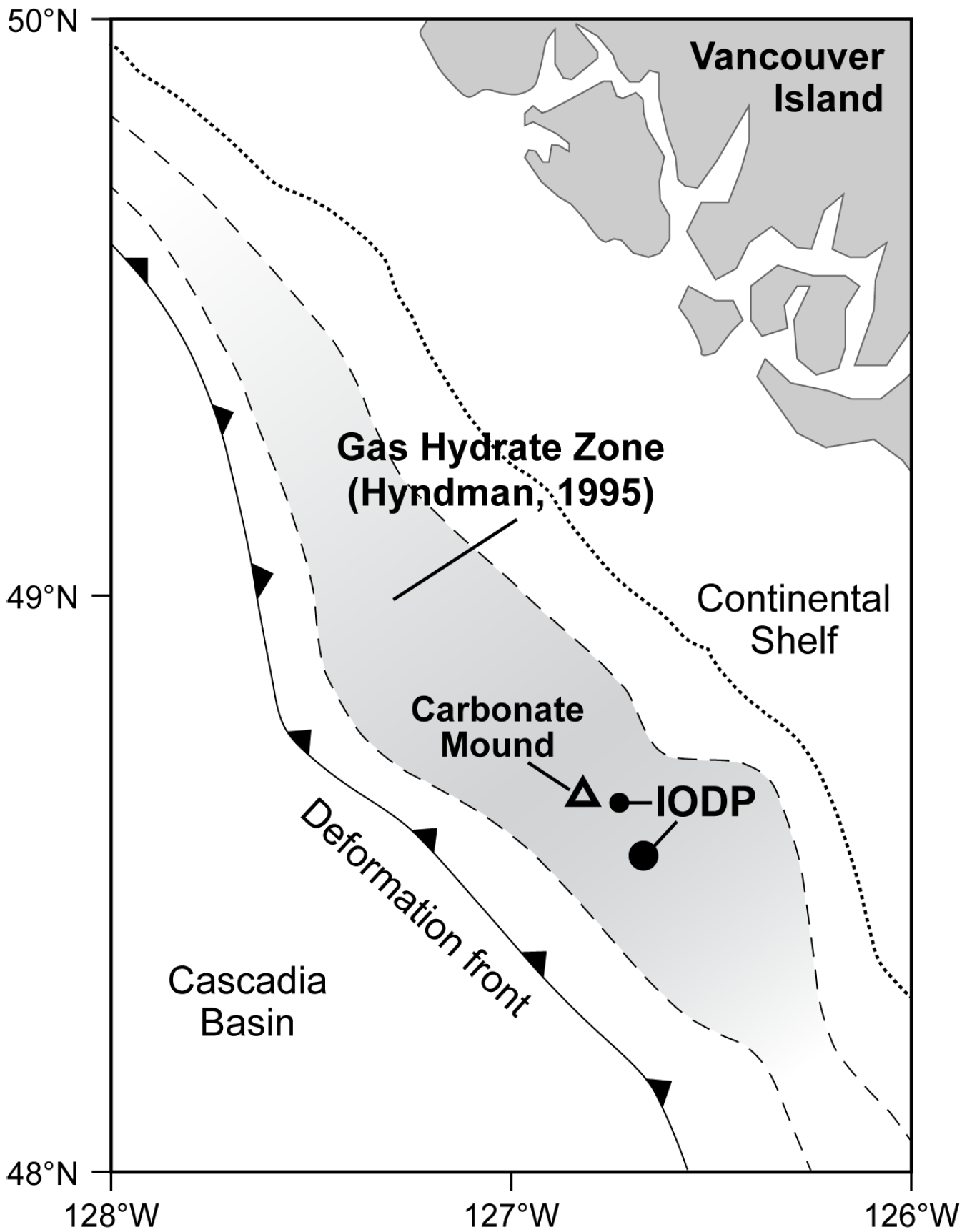
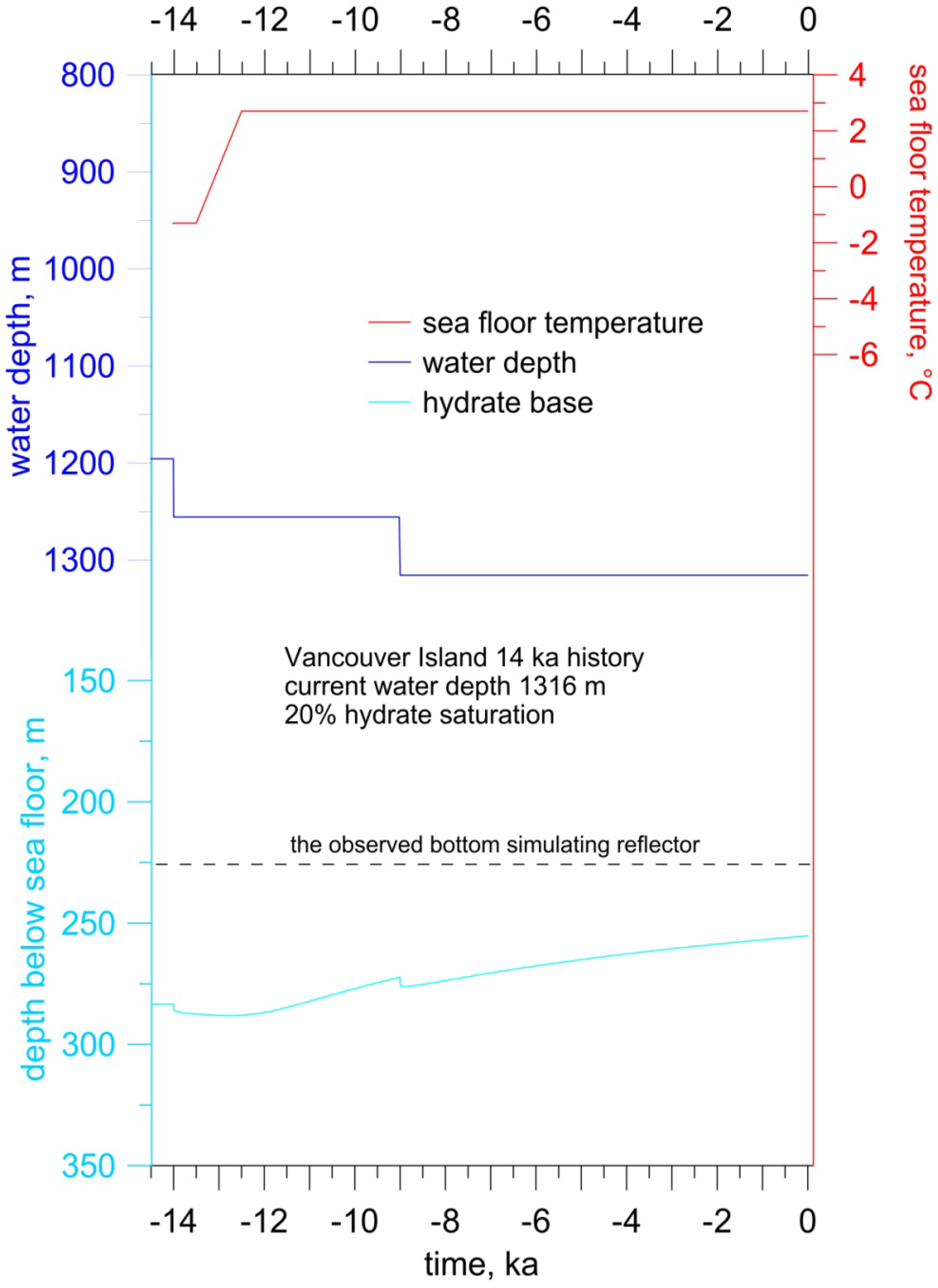
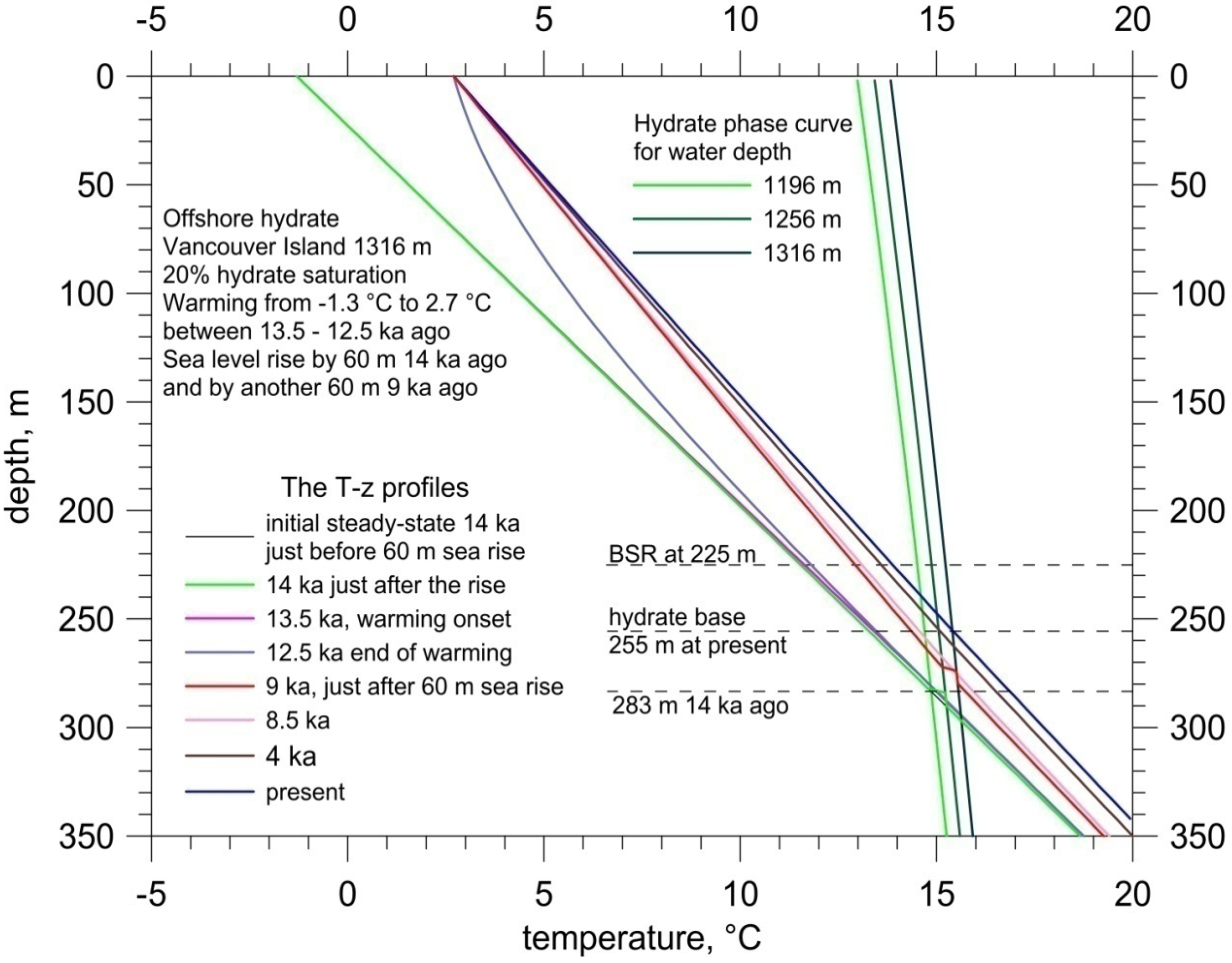
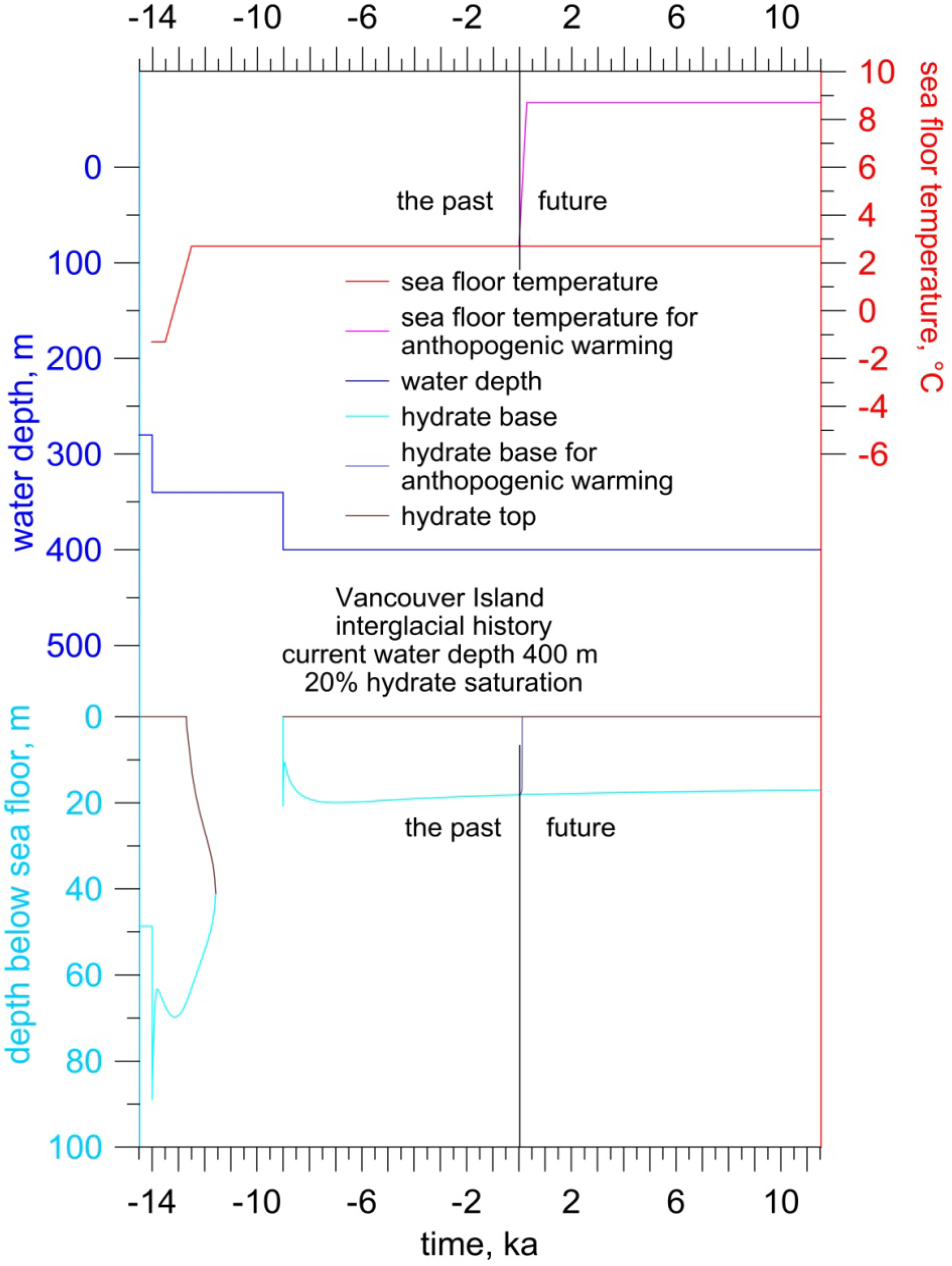
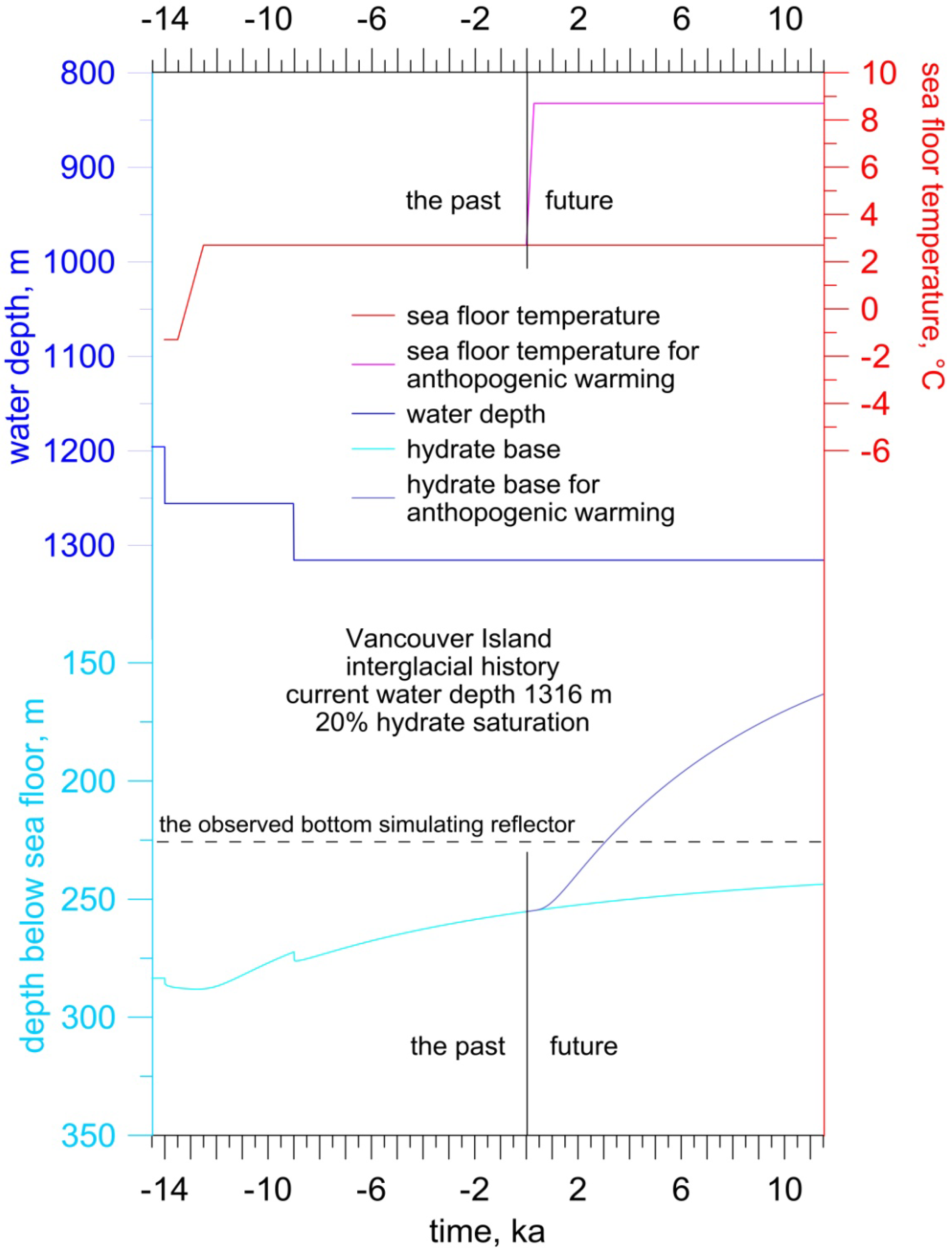
All three of our ocean margin models use inferred sea bottom temperatures and water column variations in response to glacial-interglacial cyclicity to successfully predict the current GH base consistent with observed or inferred GHs on the three oceanic margins studied. The models indicate that marine GH hydrate occurrences are locally dynamic features and the formation age and the potential methane resource volume depend significantly on the dynamics of the ocean-atmosphere system. Our models permit us to predict separately the, past, present and future responses of the GH stability zone as it responds to both natural (glacial-interglacial) and anthropogenic (climate change) forcing. On the convergent Pacific Margin, where GH is inferred pervasive the predicted GH base in deeper water is similar to previous observations from wells and previous models [10], but about 30 m deeper than the inferred base of the BSR. In deeper water the model suggests that GH have persisted there since the end of the last glacial. The shallow Pacific Margin model predicts that GHs initially dissociated completely in ~400 m water depth within ~2 kyrs the end of the last glacial because they dissociated from both the top and base of the GH layer due to the effects of sea bottom warming, but that GHs reformed after the second sea level rise 9 kyrs ago, to reach ~20 mbsf and they have thinned subsequently only slightly. Therefore we predict that Pacific Margin GHs in water depths less than ~500 m will have a younger formation age and a different history from those underlying the deeper Pacific continental shelf.

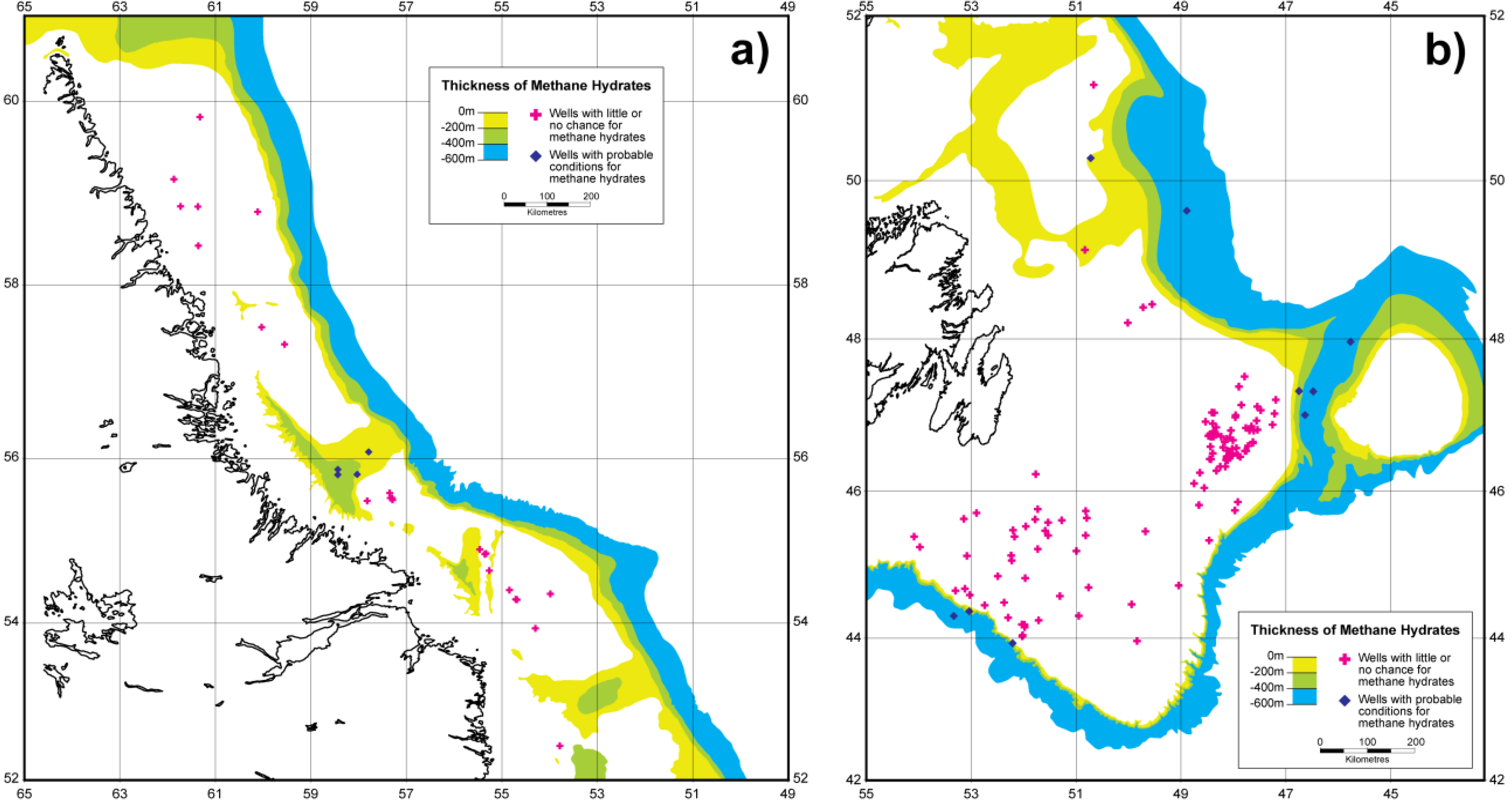
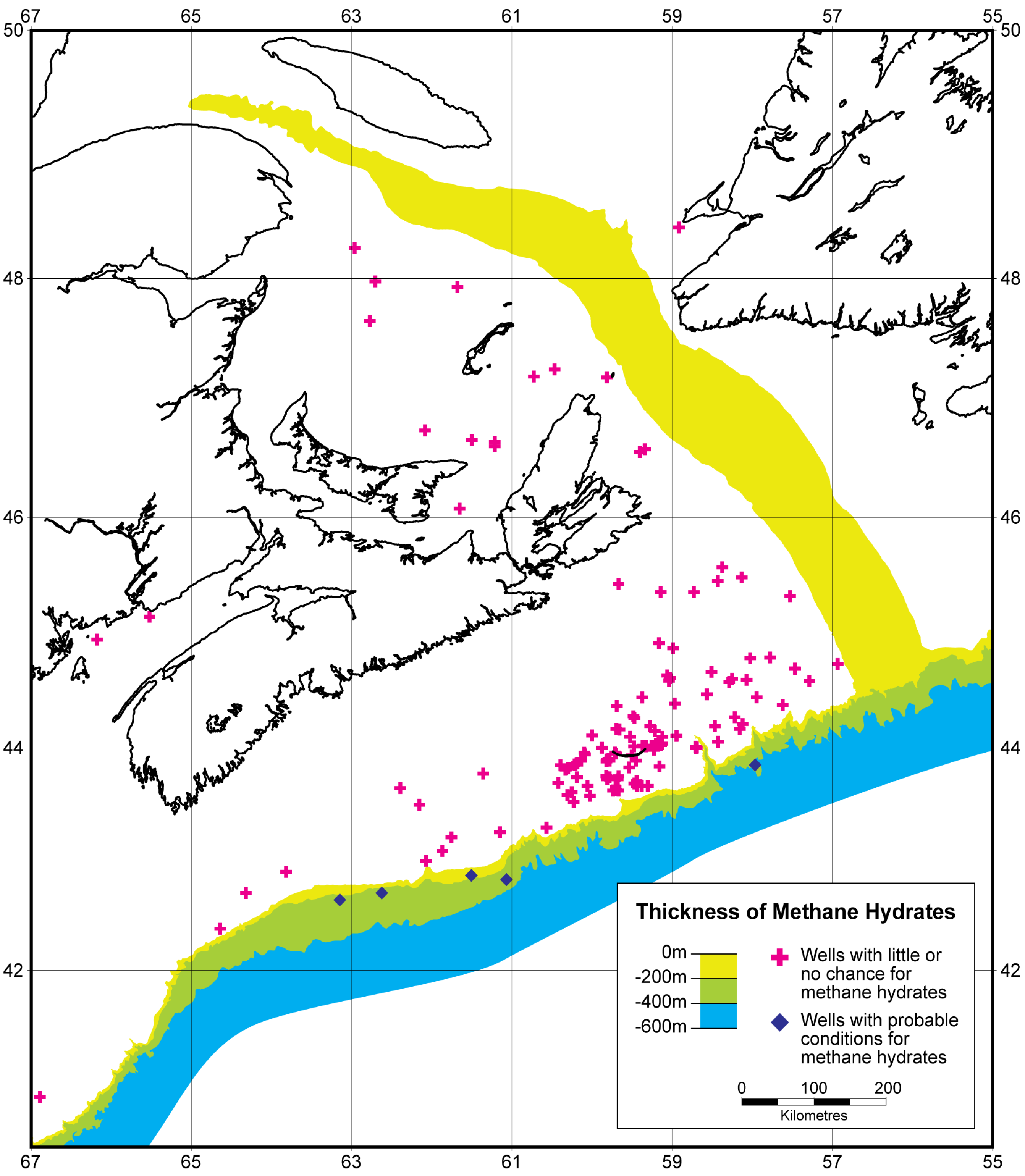
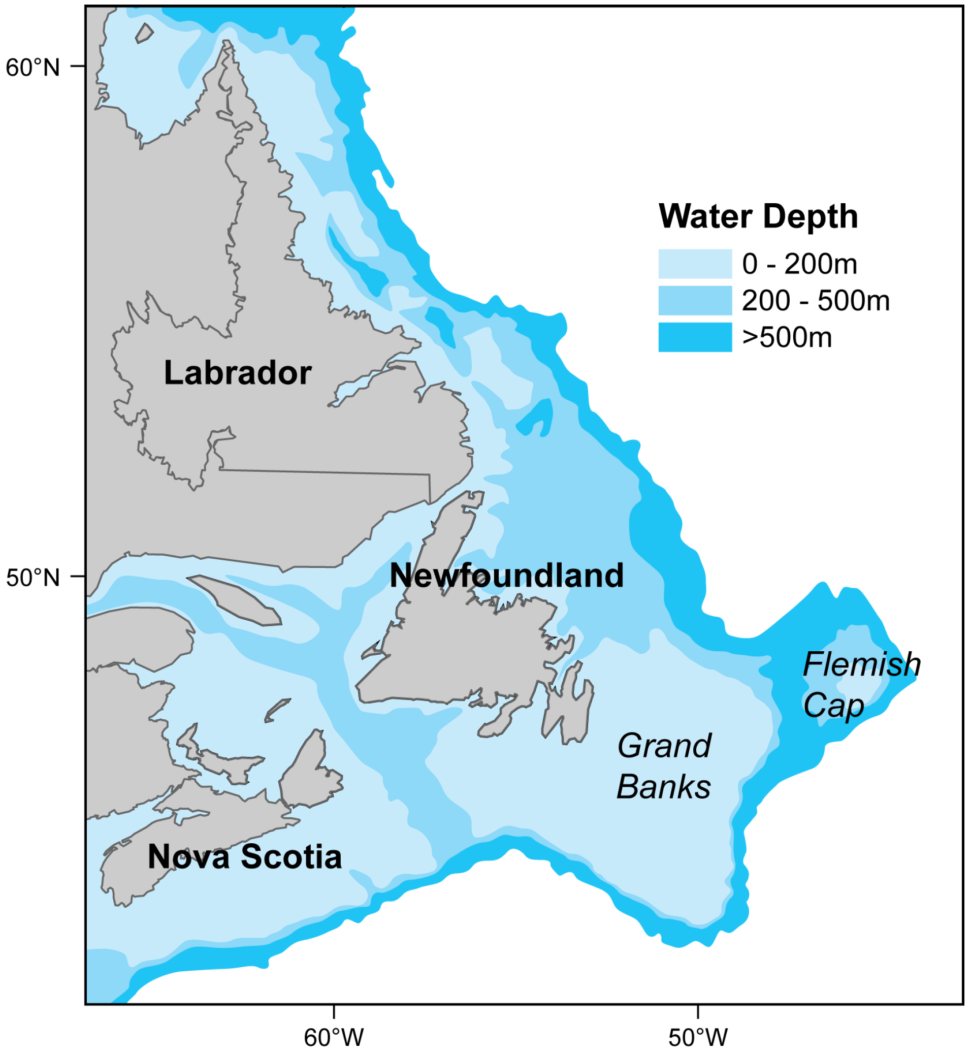
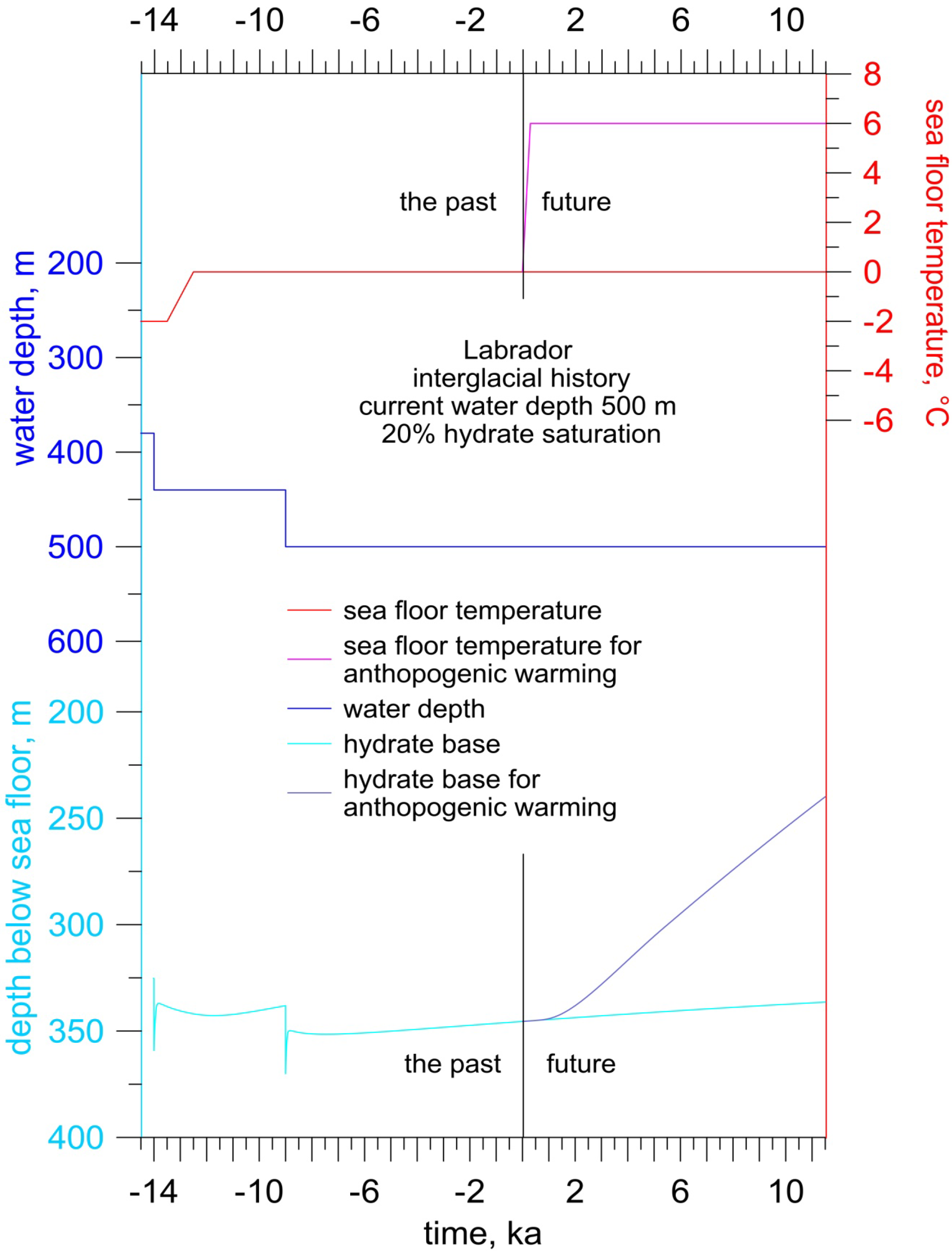
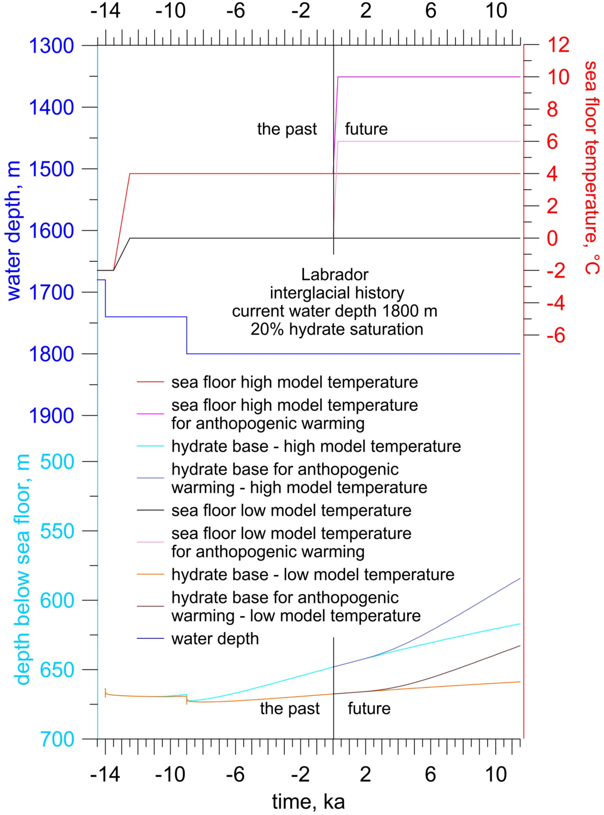
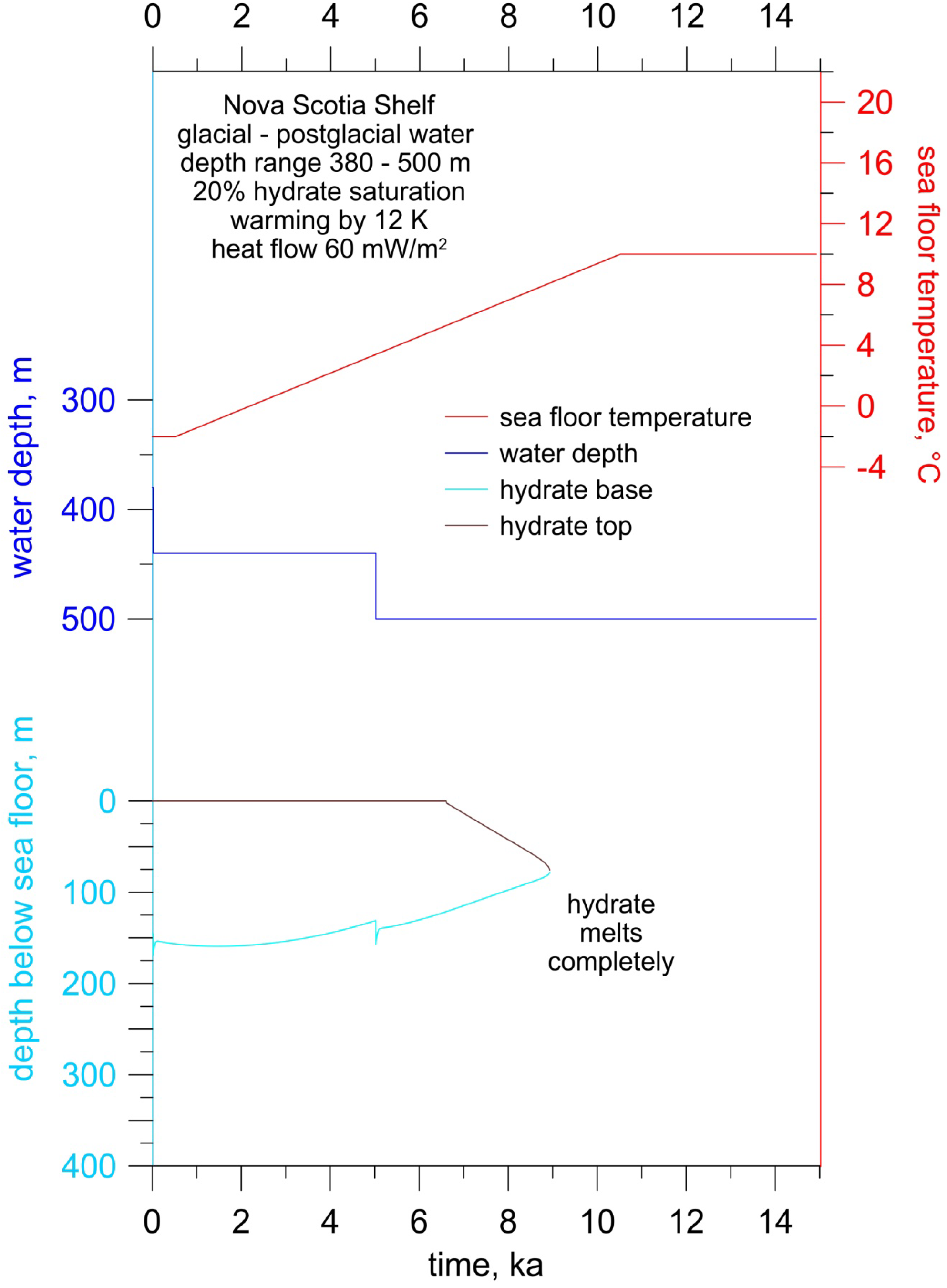
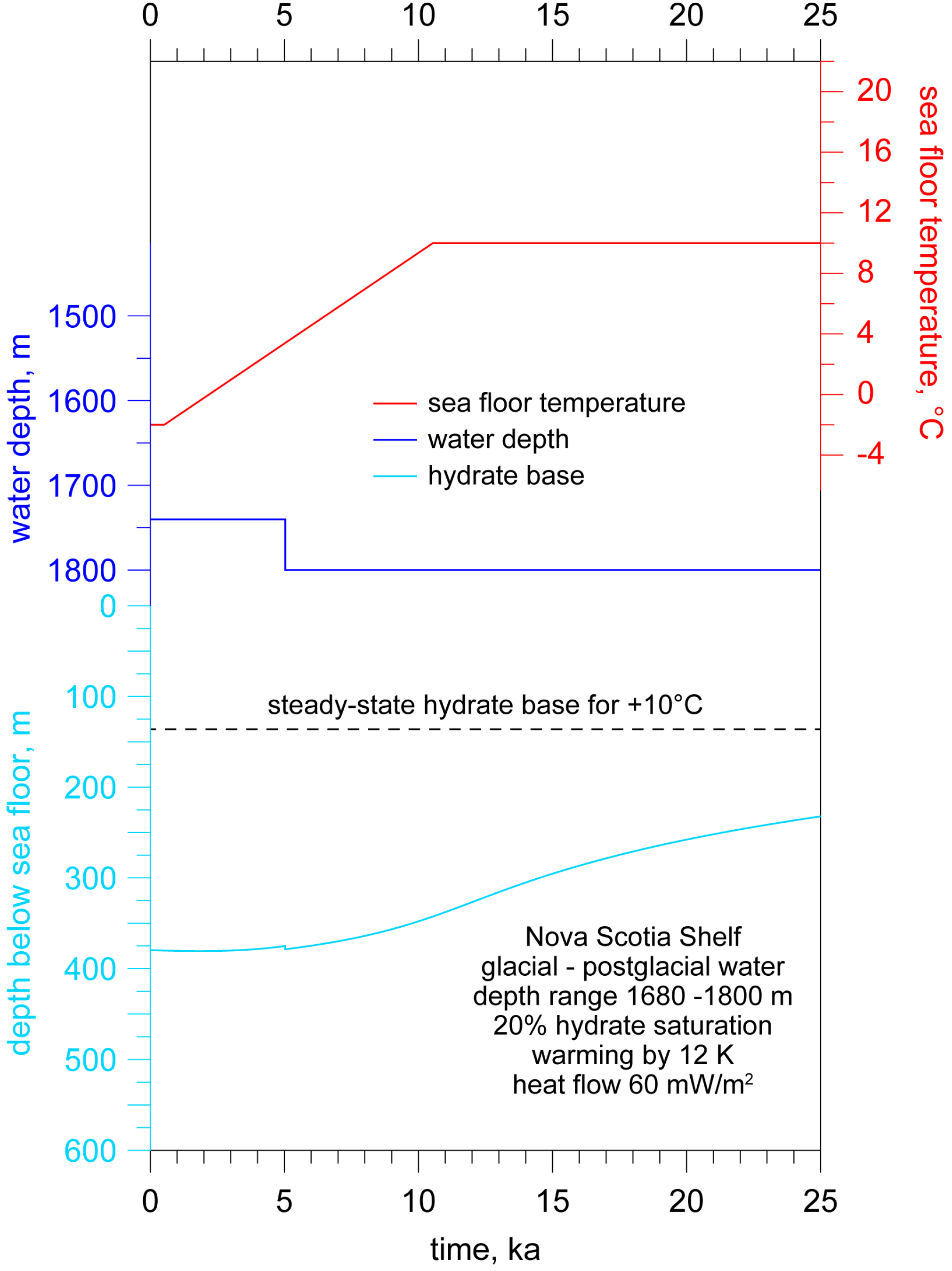
In comparison to the size of the GH stability region, GH occurrences are inferred to be rare and localized on the passive Labrador and Nova Scotia margins. BSR’s occur there occur consistently between ~400 ms and 500 ms below the seafloor, and rarely as low as 600 ms below the sea floor, where water columns are currently ~620–2550 m and sea bottom temperatures are between 0 °C and 10 °C [14,15]. Our models correctly predict an absence of GHs in the shallow, <500 m, Scotian shelf. They also predict persistent GH stability on the colder shallow Labrador shelf, where BSRs are observed rarely in water depths ~620 m [15]. Model of the deeper settings predict the current GH stability zone base between ~650 mbsf and 670 mbsf where current sea floor temperatures are 0–4 °C on the Labrador Margin and ~300 mbsf, where current sea floor temperatures are ~10 °C on the Scotian Margin. The model GH base occurs deeper than the current equilibrium depth because GH formed during the last glacial are still not in equilibrium with the modern environment. The Scotian Margin model appears consistent with Mohican Channel BSR and OBS data, which exhibits a fast-slow transition at comparable depth [15]. The Labrador model GH base appears deeper than common BSRs, ~250–445 mbsf, but it is generally similar the deepest BSR on that margin.

We inferred that the Scotian Margin GHs are relict from the last glacial, since GHs formed in equilibrium with current sea bottom temperatures are not be expected below ~130 mbsf The depth difference between model predictions on the Labrador Margin may result from any or a combination of: insufficient gas supply—as BSR are rare offshore Labrador; the age when Labrador GHs formed—as current GH base equilibrium is shallower than models relict GHs layers from the last glacial; or incorrect model assumptions. Future predictions of GH at the natural end of the current interglacial differ among the three settings because all depend significantly on sea bottom temperatures which differ among the regions studied.

7.2. Comparison of Methane Release Rates

Over time, increasing sea bottom temperature tends to reduce GH stability. The temperature change effects at the sea bottom are damped and attenuated by thermal inertia below the sea floor and phase change enthalpies. Temperature is the predominant control on GH formation and dissociation. Typically the effects are protracted, especially when GH is stable in the water column and dissociation occurs only at the GH layer base. Thus GHs on the deep Scotian slope are currently thicker than expected if they were in equilibrium. In contrast the phase change rates are accelerated significantly when GH layers dissociate from both the base and the top, when the upper GH stability limit migrates below the sea floor. Generally, as shown by the shallow Pacific and Atlantic margin models we observe the complete disappearance of GHs under these conditions on time scales of 2–9 kyrs.

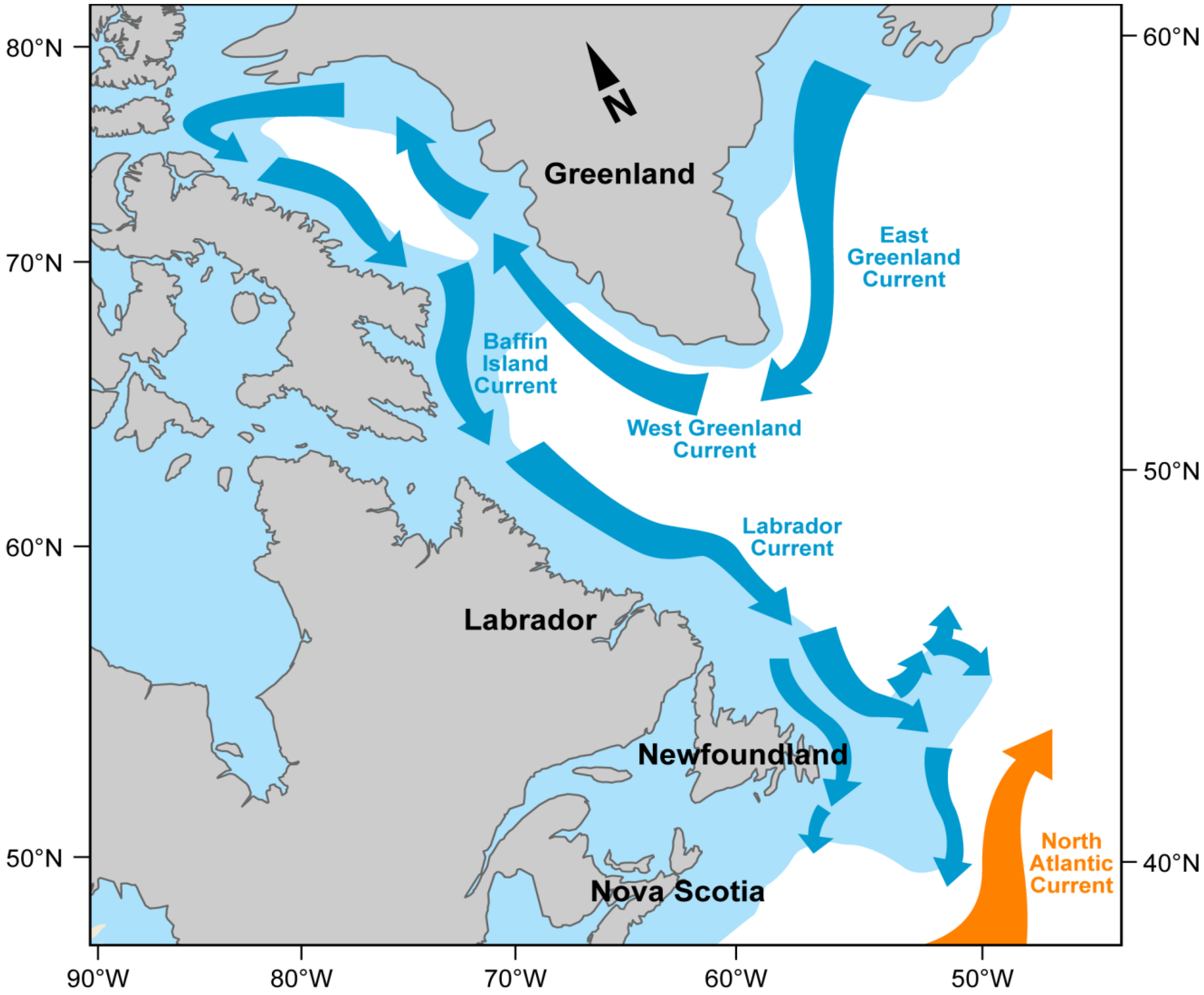
In general, all three deep water models (>1300 m) are characterized by an initial deepening of GHSZ in response to sea level rise that suppresses methane release. This lasts about 2 kyrs generally. Subsequently, thermal effects predominate and annual methane release rate increases with time. As a result the past and current dissociation rates are variable and depend on the combination of temperature predominantly, influenced also by pressure effects, more due to water depth setting than sea level rise. Methane release rates from the deep Labrador Margin are the lowest and, depending on bottom temperature model, they are less than a tenth to a half that from the Pacific Margin. The highest deep water methane release rates are from the Scotian Margin, where the deep continental shelf and slope are influenced by a warm ocean current. Methane release rates there are generally twice that of the Pacific Margin and 10–100 times that from the Labrador Margin, depending on thermal history.

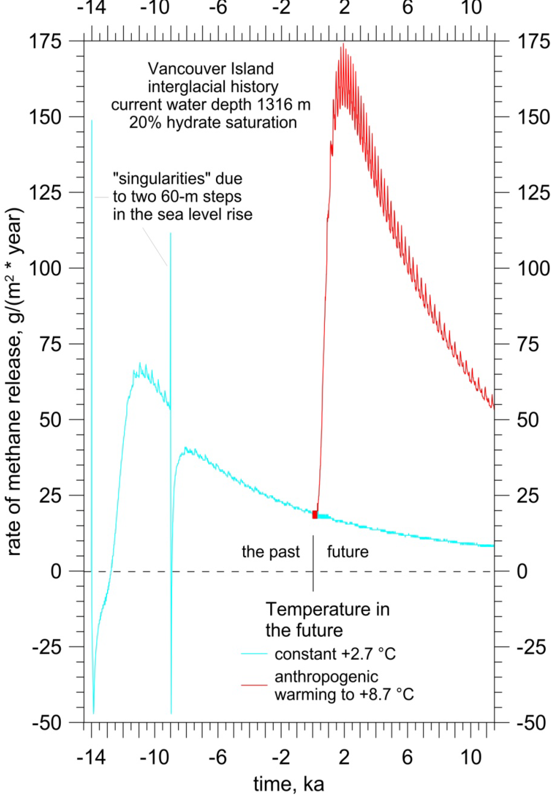
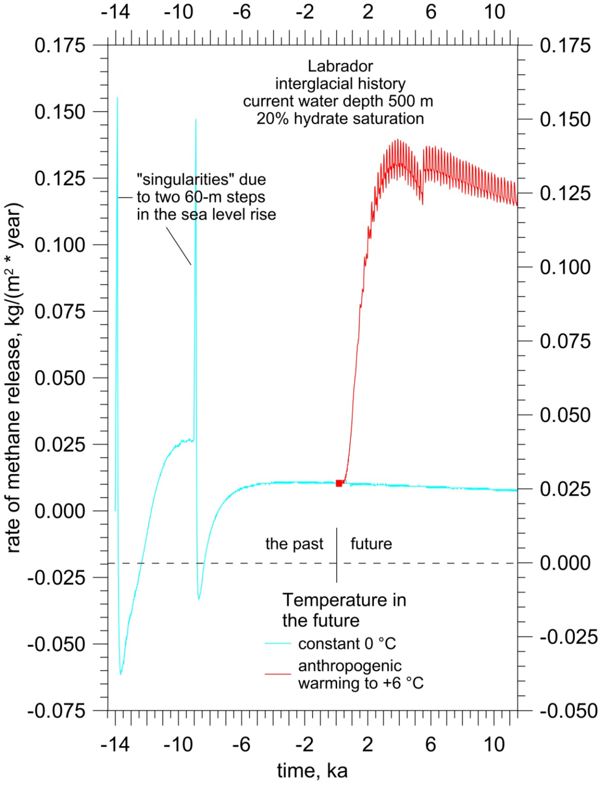
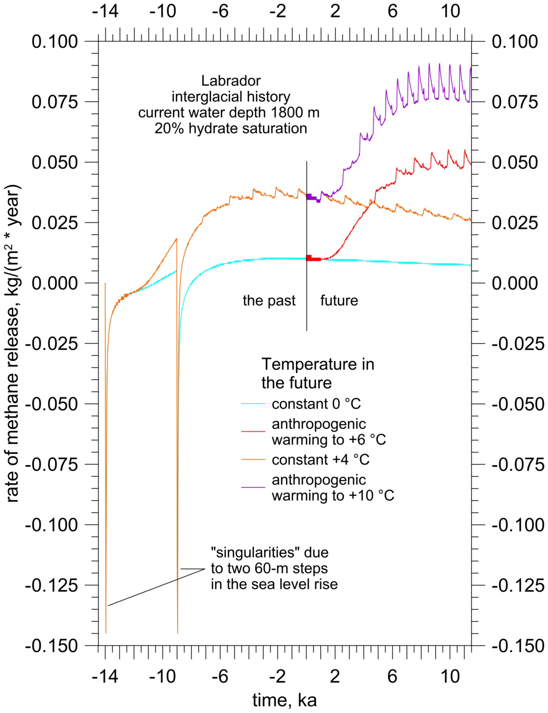
Over time, as the models approach equilibrium, the methane release rate stabilizes or declines. This change occurs first on the Pacific Margin (Figure 7), where peak methane release rates of about 0.065 kg m⁻² yr⁻¹ began to decline about ~12 kyrs ago, well before the second sea level rise step. Subsequently the annual rate declines to ~0.020 kg m⁻² yr⁻¹ currently. Initial sea level rise delays the onset of methane liberation from the deep Labrador Margin also, for ~2 kyrs after the onset of the interglacial (Figure 14). Deep Labrador methane release peaked at 0.007–0.030 kg m⁻² yr⁻¹ depending on bottom temperature model (Figure 14). 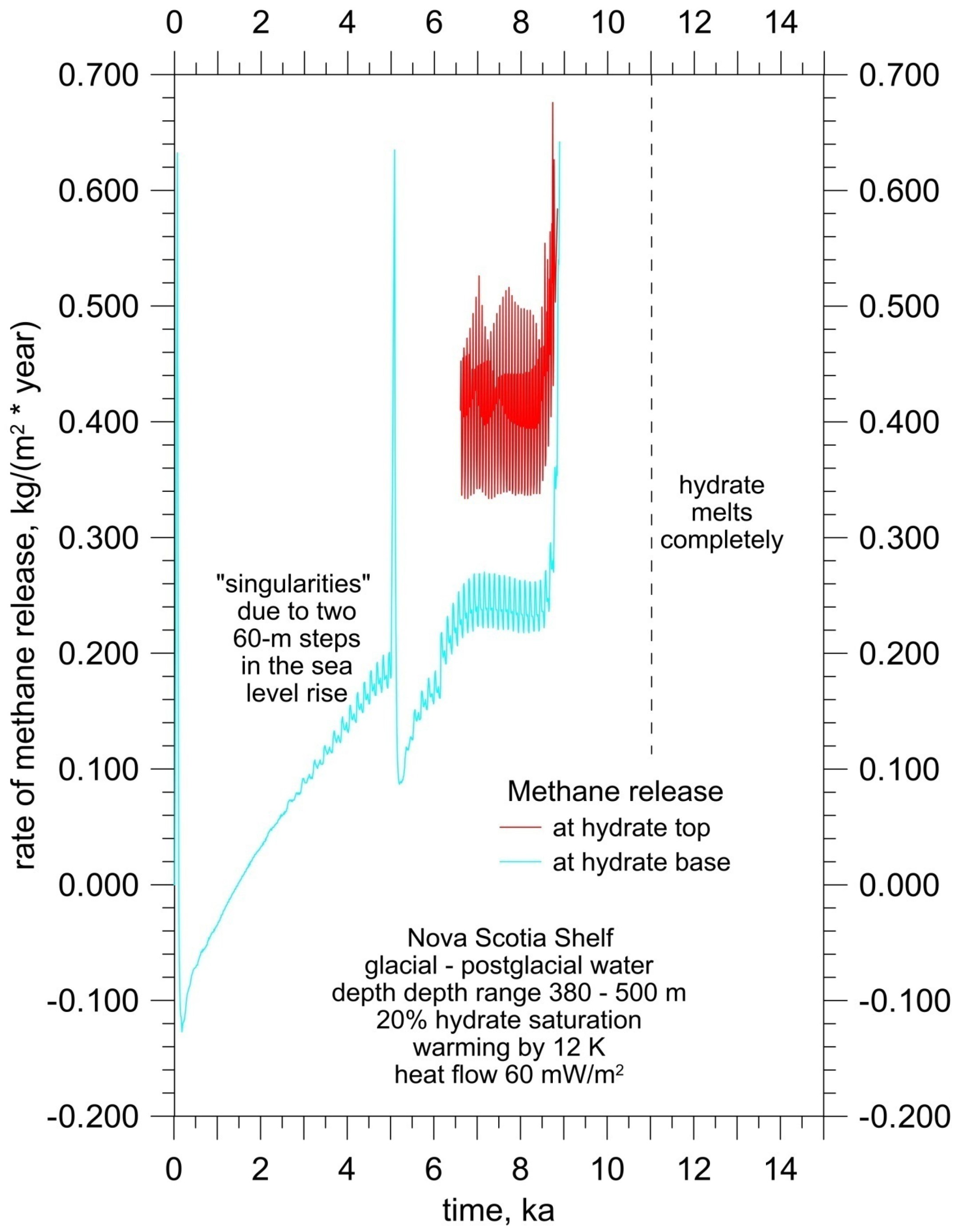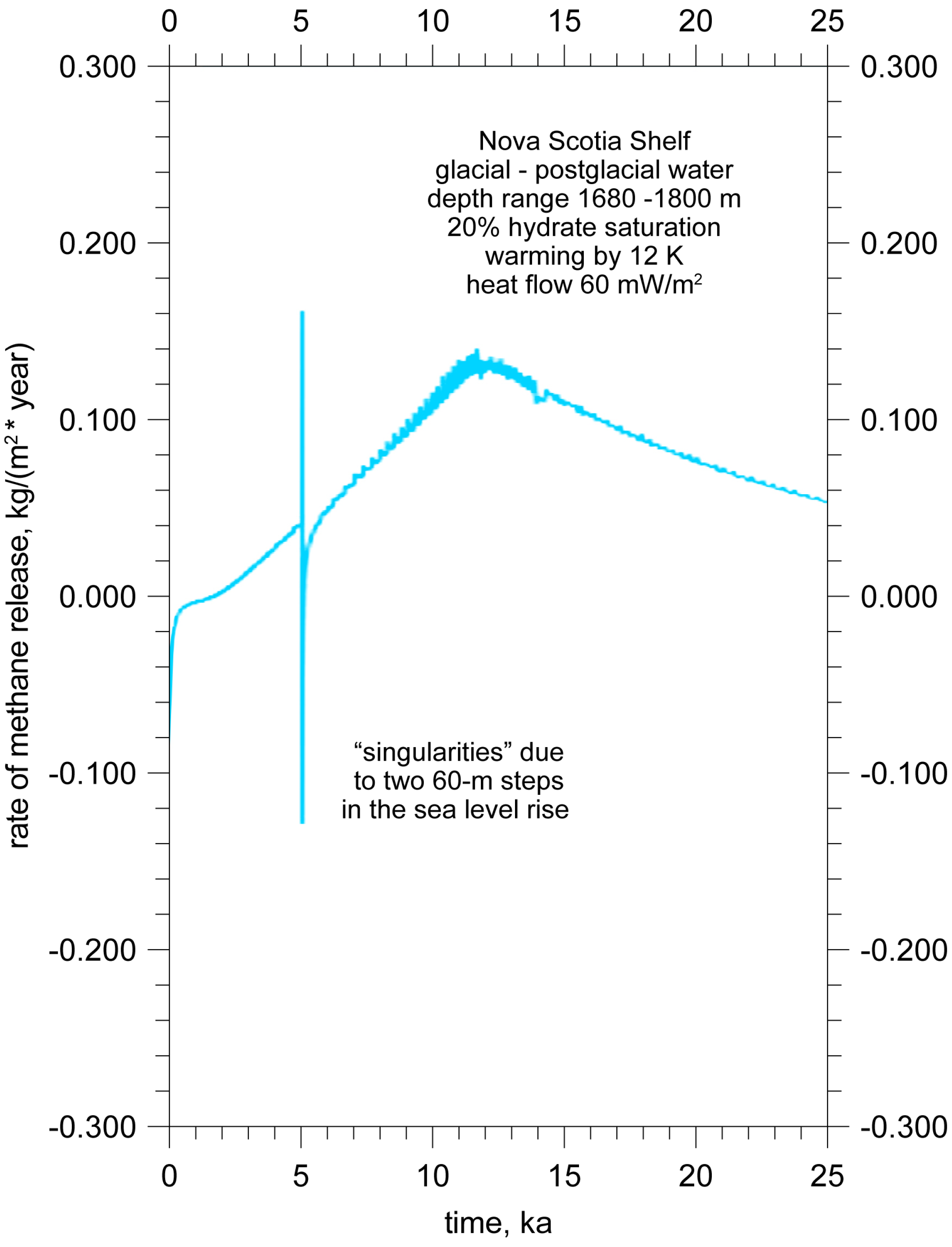Subsequently methane release resumes at a nearly constant rate from 0.010 to 0.030 kg m⁻² yr⁻¹, depending on thermal model, until today. On the Scotian Margin annual methane release rates increased throughout the interglacial to 0.13 kg m⁻² yr⁻¹ but began to decline to current annual rates of 0.110 kg m⁻² yr⁻¹ about 2 kyrs ago (Figure 19).

When projected into the future, the deep water models for all three regions illustrate that future methane release depends critically on ocean bottom temperatures. Regardless of setting the rates increase if the sea bottom temperature increases. On both the Pacific and Labrador margins, where the effects are most likely to be manifest, the annual dissociation rates increase to maximum values of between 0.175 kg m⁻² yr⁻¹ on the deep Pacific Margin and 0.080 kg m⁻² yr⁻¹ on the deep Labrador Margin, for the greatest potential ocean bottom warming considered. Should ocean bottom temperatures rise in future the resulting maximum rates in all deep settings could be almost twice current rates inferred for the deep Scotian models.

The results in shallow water, ~400–500 m, differ significantly compared to the deeper settings and amongst themselves. GHs have not been stable on the shallow Scotian Shelf for ~5 kyrs and future temperature history has no significance there (Figure 18). On the shallow Pacific Margin, the GHs that are present, formed during the interglacial in response to the second sea level rise and they are either essentially stable if sea bottom temperature is constant or they dissociate very rapidly to nearly instantaneously, ~100s of years, if sea bottom temperature rises appreciably (Figure 5). However the neo-formed GH on the shallow Pacific margin is <20 m thick and they do not represent a significant sequestered methane mass compared to the other settings. Future effects in the shallow Labrador Sea to sea bottom warming are significant, should they occur. If sea bottom temperatures there remain low then the annual methane release rate is both relatively constant and similar to the current value of 0.025 kg m⁻² yr⁻¹. However a significant warming of the shallow Labrador shelf from 0 °C to 10 °C results in a rapid, 2 kyrs, and large increase of methane release rate to 0.135 kg m⁻² yr⁻¹, which declines slightly to 0.125 kg m⁻² yr⁻¹ at the end of the current interglacial.

In summary, the previous annual marine methane release rates are highly variable depending on the water depth setting and sea bottom temperature models. The most significant increases in rate occur where the sea bottom warming is greatest. Where sea bottom temperatures remain constant the rates of methane release are lower, or declining as the system comes to thermal equilibrium. As mentioned above the future warming models employed are inferred to represent a maximum change in sea bottom temperature, and so it unlikely that the methane release rates would exceed those discussed above. Still, our models suggest that methane release from marine GHs occurs at a rate that is an order of magnitude faster than in the terrestrial permafrost environments [5,6,9,14], due in part to, their thin development adjacent the thermal boundary at the sea floor, in comparison to the buffering effects that both permafrost and greater depth exert on terrestrial gas hydrates.

7.3. Long-Term Glacial-Interglacial Cycles

Marine GHs are also a very large potential reservoir of methane and carbon. There are ~4 to ~5 times more carbon stored in marine than terrestrial GHs. The marine GH reservoir currently contains 500–10,000 giga-tonnes of carbon, with a best current estimate of 1600–2000 Gt, compared to ~400 Gt of carbon in the terrestrial sub-permafrost GH reservoir. However, as illustrated by the difference between GHs inferred on the Canadian and Pacific and Atlantic margins the global estimates of marine GHs may be exaggerated when GH base estimates are compared to actual GH occurrence as indicated by BSRs and other methods [6,15].

It is important to consider the potential impact marine GHs might have on the climate-ocean system. The immensity of the marine GH carbon reservoir combined with the rapidity with which marine GHs can dissociate in response to ocean bottom temperature changes and sea level variations suggest that GHs have a significant potential to impact the climate-ocean system. Certainly the size of the marine GH carbon reservoir and the illustrated rapidity of GH dissociation/formation suggests that GH can have a large potential impact on the climate-ocean system, but whether they actually have had an impact is more difficult to infer, primarily because of: uncertainties in the older temperature and sea level histories and the uncertainties regarding what proportion of the potential GHSZ is actually occupied by GHs as illustrated by the contrasts between the common and pervasive BSR on the Canadian Pacific Margin compared to the rate and localized BSR’s on the Canadian Atlantic Margin.

The models and discussion above focused on the more recent interglacial history since ~14 kyrs ago and on the predicted future fate and effects of marine GHs until the end of the current interglacial, ~11.5 kyrs in the future. To consider the potential role of marine GHs in climate and ocean change during the time interval from the late Pliocene to the Present requires the consideration of a much longer model interval. This is computationally possible with our model, but our previous analysis of the uncertainties in temperature history make the inference of the longer term effects of both the 41 kyrs and 100 kyrs glacial interglacial cycles uncertain. Our previous GH stability simulations in Beaufort Mackenzie region and the Canadian Arctic Archipelago [6], began in the Tertiary, but the results showed that the consideration of a long history (14.0 to 1.0 Myrs ago) had an insignificant effect on the Holocene results, such that the uncertainties attending possible alternative early temperature histories did not result in discernable variations in the current depth to the base of GHs, which is the only observable test of model validity. The extent to which local ground surface temperature (GST) or sea bottom temperature history followed regional and global variations is uncertain, especially for the more distant past. Our previous modeling [6,9], explored and tested GH formation and stability sensitivities to uncertainties in the early GST forcing model prior to the onset of the 100 kyrs glacial cycles. That sensitivity analysis compared a “warm” linearly declining, surface temperature of 10 °C, 3 Myrs ago against “cold” GST models that included 41 kyrs glacial cycles. The results differ slightly in the calculated permafrost base, but only for model intervals prior to ~1 Myrs ago. The Arctic GHs formed mainly in sub-permafrost conditions and there the model predictions for both current permafrost and GHs can be used to test model predictions. The marine GH cases considered here are controlled by sea bottom temperatures in the −2 °C to 10 °C range. Still it is useful to consider the model results for times prior to the last interglacial and a comparison of our previous Arctic models [9] to models are shown in Figure 20.

Figure 20. Comparison of the GH models for illustrated climate histories for both (1) the Canadian offshore vs. (2) the Canadian Arctic history. Curves 3 and 4 illustrate the top and bottom of the onshore Arctic GHs from [9], respectively. Curves 6 and 7 illustrate the GH layer top and bottom (below sea level) for a typical marine gas hydrate. Curve 8 illustrates the average sea bottom temperature required for GH stability below a 400 m water column assuming an average marine heat flow. The insert illustrates the GH layer top and bottom history for the shallow Nova Scotia shelf where water columns are 400–500 m thick (insert).

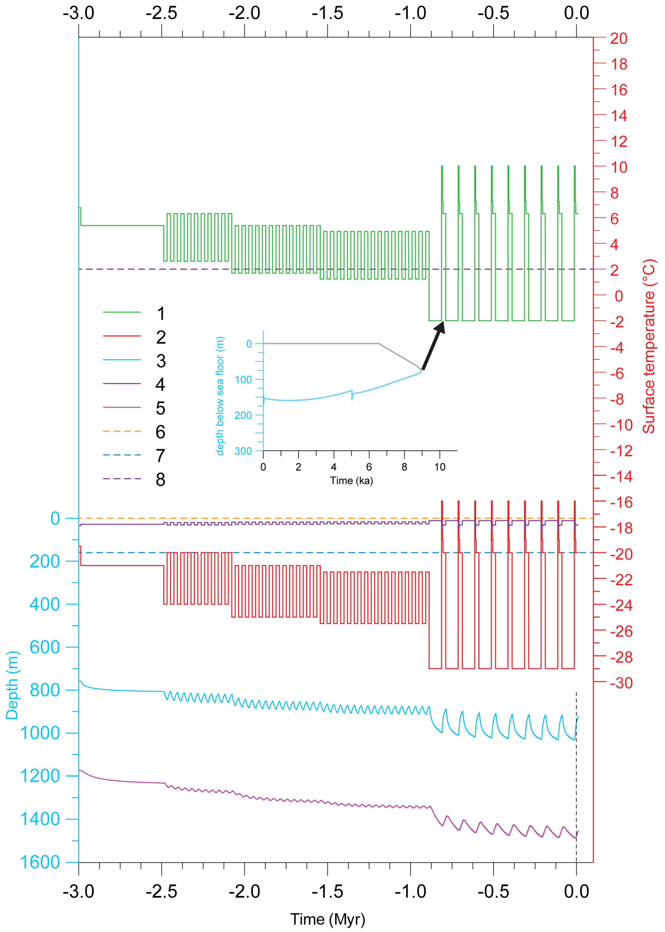
Figure 20. Comparison of the GH models for illustrated climate histories for both (1) the Canadian offshore vs. (2) the Canadian Arctic history. Curves 3 and 4 illustrate the top and bottom of the onshore Arctic GHs from [9], respectively. Curves 6 and 7 illustrate the GH layer top and bottom (below sea level) for a typical marine gas hydrate. Curve 8 illustrates the average sea bottom temperature required for GH stability below a 400 m water column assuming an average marine heat flow. The insert illustrates the GH layer top and bottom history for the shallow Nova Scotia shelf where water columns are 400–500 m thick (insert).

Temperatures were significantly, perhaps ~10 °C, higher during the interval between 14 Myrs ago and 3 Myrs ago when the 41 kyrs cycles begins and GHs would be present only where water column were >1 km on the Pacific and Labrador margins and >2 km on the Scotian Slope. Figure 20 indicates the general lack of hydrate stability conditions for most of the interval between 3.0 Myrs ago and 0.9 Myrs ago, prior to when the 100 kyrs glacial-interglacial cycles begin. Models show that the 20.5 kyrs long interglacial during the 41 kyrs glacial-interglacial cycles are sufficiently long that most marine GHs dissociate with each interglacial warming. It is therefore unlikely that GHs persisted prior to ~1.5 Myrs where water columns were <0.4 km. The analysis of the more distant past is complicated by uncertainties in both temperature and water column histories. The current temperature history uncertainty is too large to permit us to make definite and quantitative answers regarding the past effects of GHs on the climate-ocean system.

Our models show that GH stability reacts quickly to water column pressure effects but much more slowly to sea bottom temperature changes. Therefore models suggest qualitatively that GH destabilization is both responsive and progressive as sea levels fall during glacial intervals. This argues against a “catastrophic” or synchronized GH auto cyclic control on glacial-interglacial intervals. It is computationally possible; but, unfortunately in no way verifiably to analyze the interactions and impacts that marine GHs may have had prior to the current interglacial because of uncertainties in temperature and pressure history constraints. Thus we have the capability, but no confidence, that we can quantitatively contribute to questions regarding relationships among climate, glacio-eustatic sea level and marine GHs without improved temperature and water column histories. Our analysis suggests that models invoking “catastrophic” marine gas hydrate stability changes as a mechanism for climate change or oceanic anoxia are speculative, but qualitatively unsupported by our current models.

Several additional factors should be considered in models that predate the current interglacial. Warming water expands volumetrically; however, the resulting pressure is reduced by the accompanying decrease of water density with increasing temperature. Climate warming will reduce ice volumes and increase ocean volumes with higher sea levels increasing GH stability. However, it is generally inferred that continental ice sheets grow slowly compared to their melting and the rapidity of pressure effects in our models suggest that oceanic methane flux during eustatic sea level falls would be significantly delayed or retarded. Rather GH dissociation should follow falling sea level quite closely. This is contrary to the “clathrate gun” hypothesis, especially if this were accompanied by a lowering of sea bottom temperature accompanying glacial climate cycles. Thus, the situation is complex and highly dependent on the specifics of water depth, sea bottom temperatures and the actual occurrence of GHs opposed to their theoretical stability, which depends on the petroleum system. As such we must await better constraints of continental shelf petroleum system, thermal and water column histories to verifiably produce meaningful models prior to the current interglacial.

8. Conclusions

We have modeled numerically both shallow and deep regions on three Canadian oceanic margins during successive glacio-eustatic cycles to illustrate Pleistocene-Holocene marine gas hydrate stability and instability during about the last 3 Myrs, with a primary focus on the effects since the beginning of the current interglacial and projected to the “natural” beginning of the next glacial interval. Our limited temporal focus is due to uncertainties of the previous thermal and water column histories of the continental margins prior to 14 kyrs. Our models can be verified currently only against Currently inferred and observed GH occurrences, which is more successful on the Pacific Margin where GH occur pervasively, but difficult on the Atlantic and Labrador margins where BSR’s are rare. Our models demonstrate that the marine GH hydrate reservoir has dynamic features. The formation age and marine GH resource volumes depend significantly on the dynamics of the ocean-atmosphere system. Our models show that marine GH respond to both natural (glacial-interglacial) and anthropogenic (climate change) forcing. Based on the general agreement of current model predictions and the inferred or identified GH occurrences on Canadian continental shelves we infer that our models can illustrate reliably the history of these marine GHs within the accuracy of the oceanic environmental constraints that are available.

During the current interglacial the thickness of the GHs on Canadian oceanic margins have responded uniquely since the end of the last glacial. The responses differ based on the combination of position as it controls water depth history and the change in sea bottom temperatures influenced strongly by ocean currents. The effects of glacio-eustatic sea level rise are minor. They last about 2 kyrs and punctuate the longer and predominant effects of sea bottom temperature change which propagates downward into the GH layer. In general, the GH stability zone in the deeper (>1316 m) parts of the Pacific and Atlantic margins has thinned in response primarily to increased water bottom temperatures, but GH remain stable there now and until the end of the current interglacial.

On the shallower (400–500 m) continental shelf the GH stability history is highly variable. On the Pacific Margin shallow GH were completely dissociated prior to 9 kyrs ago, but the effects of subsequent sea level rise reestablished a thin GH stability zone that persists. On the Scotian Shelf GH stability disappeared completely under the influence of the warm Gulf Stream, whereas offshore Labrador the cooling effects of the Labrador current and sea level rise served to increase shallow water GH stability there until nearly the Present.

If future ocean bottom temperatures remain constant the general marine GH characteristics persist to the end of the current interglacial, but if the sea bottom warms there could be a significant reduction to complete loss of GHs, especially from the shallower continental shelf. The interglacial GH thinning rates, both past and future, constrain the range of rates at which carbon may be transferred between the GH and atmosphere-ocean system. The previous annual marine methane release rates are highly variable depending on the setting and sea bottom temperature models. The most significant rate increase occurs where the sea bottom warming is greatest. Where sea bottom temperatures remain constant the rates of methane release are lower, or declining as the system comes to thermal equilibrium. The models suggest that methane is release from marine GHs occurs at a rate that is an order of magnitude faster than that of terrestrial permafrost environments [5,6,9,14]. This, combined with the immensity of the marine gas hydrate carbon reservoir suggests that GH have the potential to contribute to changes in climate-ocean system.

Our models show that GH stability reacts quickly to water column pressure effects but slowly to sea bottom temperature changes. Therefore it is likely that GH destabilization was both responsive and progressive to sea level fall during glacial intervals, which suggests against a catastrophic GH auto-cyclic control on glacial-interglacial intervals. It is computationally possible; but, unfortunately in no way verifiably, to analyze the interactions and impacts that marine GHs had prior to the current interglacial because of uncertainties in local specific temperature and pressure history constraints. Thus we have the capability, but no confidence, that we can contribute to questions regarding relationships among climate, glacio-eustatic sea level and marine GHSZ without improved temperature and water column histories. Our analysis suggests that models invoking “catastrophic” marine gas hydrate stability changes as a mechanism for climate change or oceanic anoxia are speculative and qualitatively unsupported by our models.