Harmonic Loss Analysis of the Traction Transformer of High-Speed Trains Considering Pantograph-OCS Electrical Contact Properties

Abstract

The traction transformer of the traction drive system of a high-speed train is one of the main equipments for energy conversion. The transformer loss will be increased by load harmonics and pantograph arcs at high speed. It is very important to predict losses for the improvement of traction transformer design. In this paper, a dynamic model of the pantograph-catenary system is established using the MSC.Marc software based on the finite element method to analyze disconnection events in different speeds. Then the pantograph arc, traction transformer and four-quadrant converter model is set up. Resistance variations with the change of harmonic frequency have been considered in the calculation formulae of harmonic losses. Traction transformer losses can be calculated based on the harmonic T-equivalent circuit and superposition principle. Considering the harmonic losses variations, the effects of arc voltage on harmonic copper loss and harmonic core loss are analyzed, respectively. The average loss at different disconnection ratios is also calculated. This method could be used to estimate the increment of transformer harmonic losses with poor current conditions at high speed.

1. Introduction

Compared with other vehicles, high speed trains have the advantages of high efficiency, energy savings and low emissions. For example, the energy consumption per hundred kilometers per person of the Chinese CRH380A train is only about 4.6 kWh [1]. In Europe, Japan, China and other places, high-speed railways have become an important mode of transportation. Analysis of the losses of every part of a high-speed train traction drive system in detail in order to improve the efficiency further is of significant importance. The traction drive system of the high-speed train accepts AC 25 kV, 50 Hz power from the pantograph-Overhead Contact System (OCS). The vacuum circuit breaker (VCB) connects the AC power to the primary winding of the traction transformer, and then the secondary windings output low voltage AC power to the four-quadrant converter which can supply the traction energy to the traction motor and transmit the regenerative braking energy to the power grid during the inverter condition. Therefore, the traction transformer is a significant part of the energy transmission system, and its losses account for a larger percent of the total losses of the traction drive system. It has a realistic and economic significance to study the addition losses cause by harmonics for energy conservation. Pulse width modulation (PWM) voltage control is widely used in the four-quadrant converter, which makes the traction transformer run in the harmonics environment. The current harmonics will induce additional losses in the windings. Furthermore, under cold weather conditions, decreasing load or at higher speed, the arcing between the pantograph and the contact wire will be more predominant [2,3]. The pantograph arc generates transients, cause asymmetries and distortions in supply voltage and current waveforms [2,3,4,5]. The asymmetry generates voltage harmonics which cause harmonic core losses of the traction transformer. In-depth understanding of the harmonic losses is important for estimating harmonic losses and improving the energy efficiency in traction transformers.

The harmonic losses of transformer operated by PWM inverters have studied in the literature [6,7]. Distribution transformer and HVDC converter transformer losses caused by harmonic loads have been calculated in [8,9], respectively. All the researches above focus on the analysis of transformer losses caused by harmonic loads or unbalanced loads, whereas high-speed train traction transformer losses caused by poor current collection from the pantograph-OCS at high speed have drawn little attention. For the calculation of losses, finite element simulation software is widely used to emulate the harmonic copper losses [10,11] and harmonic core losses [12,13,14,15,16]. This approach can accurately calculate the relative transformer losses, but many nonlinear parameters must been known in modeling and post-processing in finite element simulation software in order to get more accurate simulation results, such as the magnetizing curve, loss curves with different frequency, and physical dimensions, etc. [17]. Therefore its complexity determines that this method is not convenient to apply. Consequently, the winding resistance and excitation resistance in a traditional T-equivalent circuit model could reflect copper losses and core losses, respectively. Harmonic losses could be calculated by the product of harmonic current and resistance, but variations of resistance values with harmonic frequency are not considered, so an advanced T-equivalent model [18], considering change of winding resistance and excitation resistance with harmonic frequency, has been set up in this paper. This method is simple and effective and could be easily programmed.

In this paper, the dynamic model of a pantograph-catenary system has been established and disconnection events can be obtained from contact pressure curves at different speeds using the MSC.Marc simulation software (MSC.Software Corporation, Santa Ana, CA, USA). We have set up a pantograph arc, traction transformer and four-quadrant converter model and carry out simulations using MATLAB/SIMULINK. Considering resistance variations with the change of harmonic frequency and using the advanced T-equivalent circuit and superposition principle, we have analyzed the effects of arc voltage and disconnection events on harmonic copper and core losses, respectively.

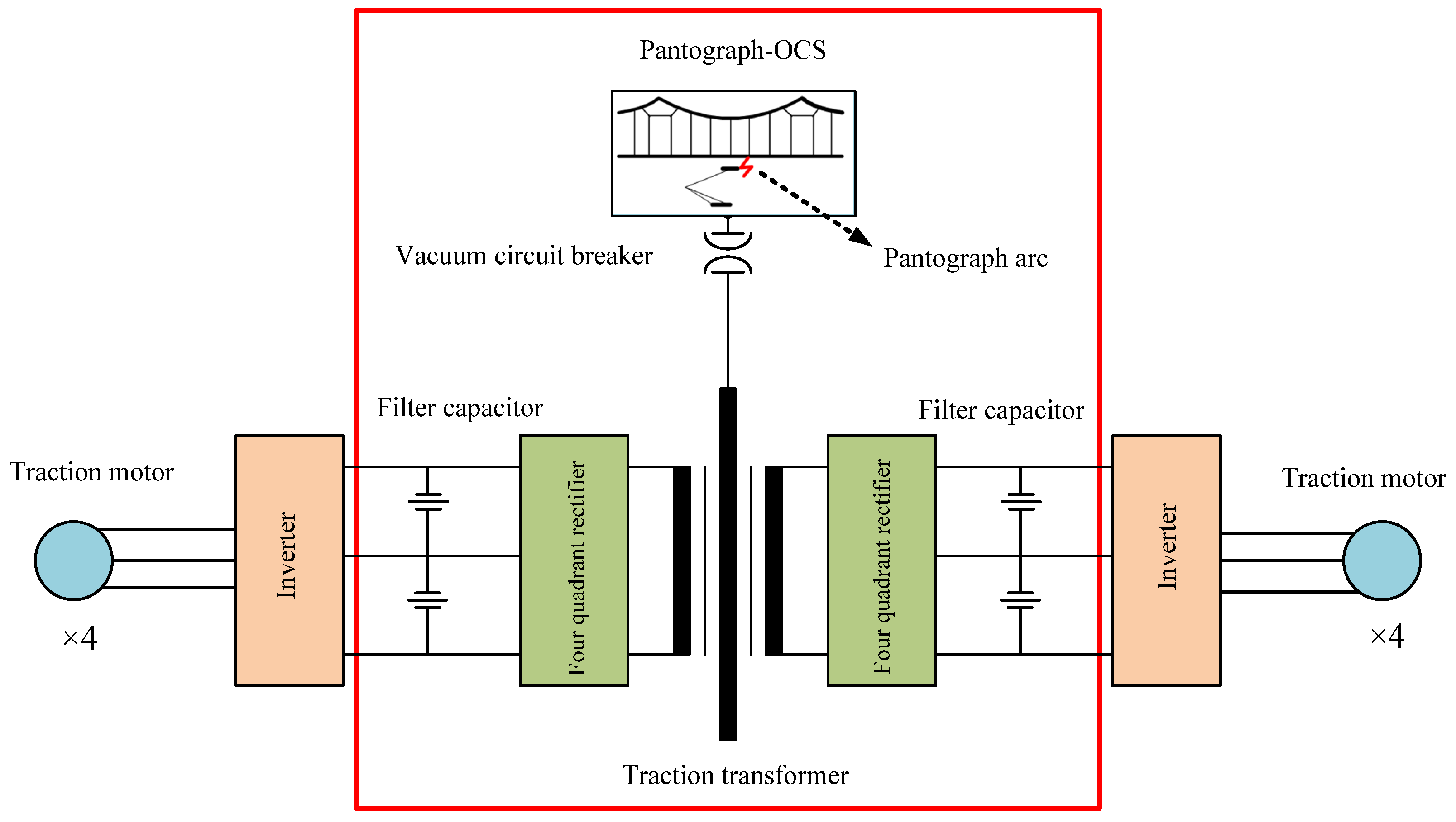
2. Analysis of the Traction Drive System

Figure 1 show the traction drive system of a high-speed train, which is composed of a traction transformer, two four-quadrant converters, two inverters and eight traction motors. The traction transformer has a primary winding and two traction windings. Each of traction windings of the transformer has been connected with a four-quadrant converter, an inverter and four traction motors. The pantograph-OCS provides the impetus input for high speed trains, and power transmission depends on the good contact between pantograph and contact wires. The traction transformer transfers AC 25 kV, 50 Hz current obtained from the pantograph to the three-level four-quadrant converter. The PWM control method could achieve regulable DC voltage control and the unit power factor control of the primary side. The four-quadrant converter could feed back power through the traction transformer to the power grid under regenerative braking working conditions. The DC voltage is transformed by the inverter into frequency and amplitude adjustable AC voltage to supply the traction motors.

Figure 1. Traction drive system of a high speed train.

Figure 1. Traction drive system of a high speed train.

2.1. Pantograph-OCS

High speed trains can accept power from the sliding contact between the pantograph slide and contact wires. When the running pantograph is passing by the relatively static catenary, the contact wires suffer from external interference, so a dynamic interaction is generated between the pantograph and the catenary. As the speed increases, vibration become serious, and can force the pantograph slide away from the contact wires and generate arcs and sparks. In addition, the contact wires become covered with a thin layer of ice in winter, which also causes poor contact and arc generation. The nonlinear characteristics of arcs between the pantograph and the catenary causes line voltage distortions. Moreover, the contact loss will directly affect the current collection, and even cause instantaneous power supply interruptions, which cause a loss of train traction and braking force. This paper has set up a pantograph-catenary finite element model and classic arc model for subsequent analysis.

2.1.1. Disconnection Events

The contact wires and pantograph are unrelated, but they are interrelated and interact with each other only while they are moving. The bond between the pantograph and catenary is the uplift force and contact pressure. This paper has regarded the interaction force as a research object and established a catenary and pantograph model.

The motion equations of contact wires can be described as below [19]:

$$m_c\frac{{\partial }^2{u}_c}{\partial t^2}+\frac{{\partial }^2}{\partial x^2}(E{I}_c\frac{{\partial }^2{u}_c}{\partial x^2})-\frac{\partial }{\partial x}(T_c\frac{\partial u_c}{\partial x})-k_d(u_m-u_c)\delta (x-x_n)=F\delta (x-Vt)$$

(1)

where, m_c, EI_c, T_c and k_d express the unit mass, flexural rigidity, tension force and hanger stiffness of the contact wires; δ is the impact function; F expresses the contact pressure between the pantograph and catenary, which is the sum of the static contact pressure and dynamic contact pressure; u_c is the displacement of the contact wires; u_m is the displacement of the carrying cable; x_n expresses the distance between the hanger and motion point; x is the motion point; t is time and V is speed.

The motion equations of the carrying cable can be obtained as below [19]:

$$m_m\frac{{\partial }^2{u}_m}{\partial t^2}+\frac{{\partial }^2}{\partial x^2}(E{I}_m\frac{{\partial }^2{u}_m}{\partial x^2})-\frac{\partial }{\partial x}(T_m\frac{\partial u_m}{\partial x})+k_d(u_m-u_c)\delta (x-x_n)+k_s{u}_m\delta (x-x_s)=0$$

(2)

where, m_m, EI_m, and T_m express the unit mass, flexural rigidity, tension force and hanger stiffness of the carrying cable; k_s is the equivalent stiffness of the support device, x_s expresses the distance between the support point and motion point; x is the displacement of the motion point.

The 3-degree spring model of pantograph can be expressed as:

$$\{\begin{array}{l}{M}_1\frac{{\partial }^2{y}_1}{\partial t^2}+C_1(\frac{\partial y_1}{\partial t}-\frac{\partial y_2}{\partial t})+K_1(y_1-y_2)+R_{1}sign(\frac{\partial y_1}{\partial t}-\frac{\partial y_2}{\partial t})=-F_c\\ M_2\frac{{\partial }^2{y}_2}{\partial t^2}+C_1(\frac{\partial y_2}{\partial t}-\frac{\partial y_1}{\partial t})+K_1(y_2-y_1)+R_{1}sign(\frac{\partial y_2}{\partial t}-\frac{\partial y_1}{\partial t})+\\ C_2(\frac{\partial y_2}{\partial t}-\frac{\partial y_3}{\partial t})+K_2(y_2-y_3)+R_{2}sign(\frac{\partial y_2}{\partial t}-\frac{\partial y_3}{\partial t})=0\\ M_3\frac{{\partial }^2{y}_3}{\partial t^2}+C_2(\frac{\partial y_3}{\partial t}-\frac{\partial y_2}{\partial t})+K_1(y_3-y_2)+R_{2}sign(\frac{\partial y_3}{\partial t}-\frac{\partial y_2}{\partial t})+C_3\frac{\partial y_3}{\partial t}+R_{3}sign(\frac{\partial y_3}{\partial t})=F_{C0}\end{array}$$

(3)

where, M_i, K_i, C_i, R_i, y_i (i = 1, 2, 3) express the equivalent mass, equivalent stiffness, equivalent dampening, dry friction and displacement of the pantograph head, upper frame and lower frame; F_c0 and F_c express the static contact pressure and dynamic contact pressure, respectively [20,21].

According to Equations (1)–(3), the pantograph-catenary finite element model can be established using the MSC.Marc software. Figure 2 shows the coupling model of the pantograph-catenary system. According to the parameters of the Beijing-Tianjin high-speed railway in China, and ignoring the influence of air turbulence on the vibration between the pantograph and catenary, contact pressure curves in different speeds can be obtained (Figure 3).

Figure 2. Pantograph-catenary system model.

Figure 2. Pantograph-catenary system model.

Figure 3. (a) Contact pressure curves of 250 km/h; (b) Contact pressure curves of 350 km/h; (c) Contact pressure curves of 400 km/h; and (d) Contact pressure curves of 450 km/h.

Figure 3. (a) Contact pressure curves of 250 km/h; (b) Contact pressure curves of 350 km/h; (c) Contact pressure curves of 400 km/h; and (d) Contact pressure curves of 450 km/h.

Take four sets of data in different speed as an example. Details have been shown in Table 1. The total time t_total is the whole simulation time except for the pantograph rising time. Disconnection-time t_loss is the sum of every disconnection, which is described as the 0 N contact pressure. t_total minus t_loss is contact-time t_contact. The contact pressure is greater than 0 N during the contact-time t_contact. Therefore, the ratio of disconnection p_loss can be expressed as p_loss = t_loss/t_total. From Figure 3, it can be found that the number of points with contact pressure curves equaling 0 is rising with increasing speed, which suggests that the amount of disconnection-time is increasing too. The disconnection ratio p_loss in Table 1 is consistent with the above results. The international standards demand that the disconnection ratio should not be greater than 5%. In Table 1, p_loss is less than 5% while the speed is under 350 km/h, but when the speed reaches 400 km/h or more higher, the disconnection ratio is larger than 20%, which is not allowed.

Table 1. Disconnection data.

Speed (km/h)	tloss (s)	tcontact (s)	ttotal (s)	Ratio of disconnection ploss
250	0.018	4.112	4.13	0.44%
350	0.1029	2.8771	2.98	3.45%
400	0.5513	2.0187	2.57	21.45%
450	0.67	1.67	2.34	28.63%

Table 1. Disconnection data.

Speed (km/h)	tloss (s)	tcontact (s)	ttotal (s)	Ratio of disconnection ploss
250	0.018	4.112	4.13	0.44%
350	0.1029	2.8771	2.98	3.45%
400	0.5513	2.0187	2.57	21.45%
450	0.67	1.67	2.34	28.63%

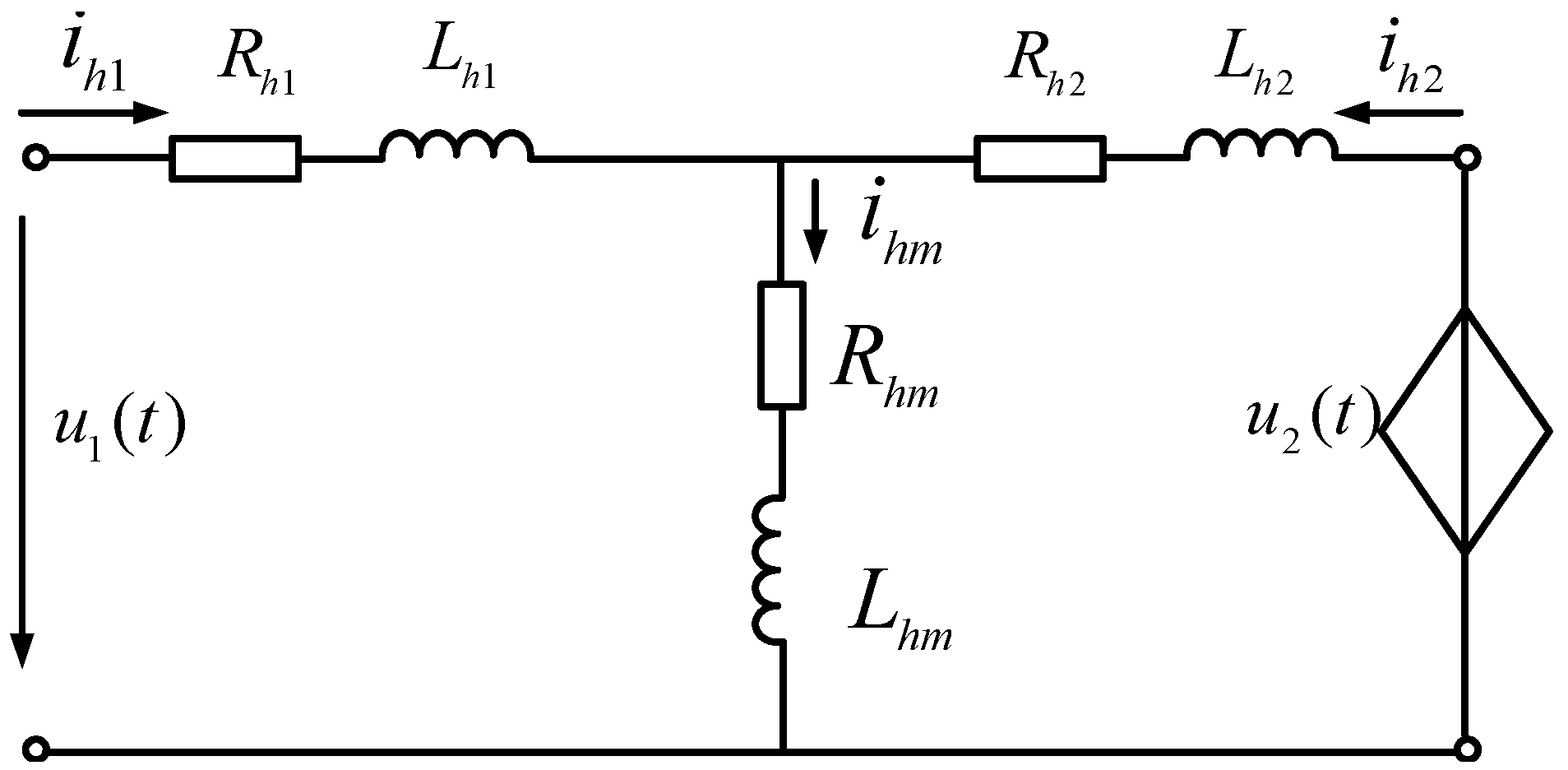
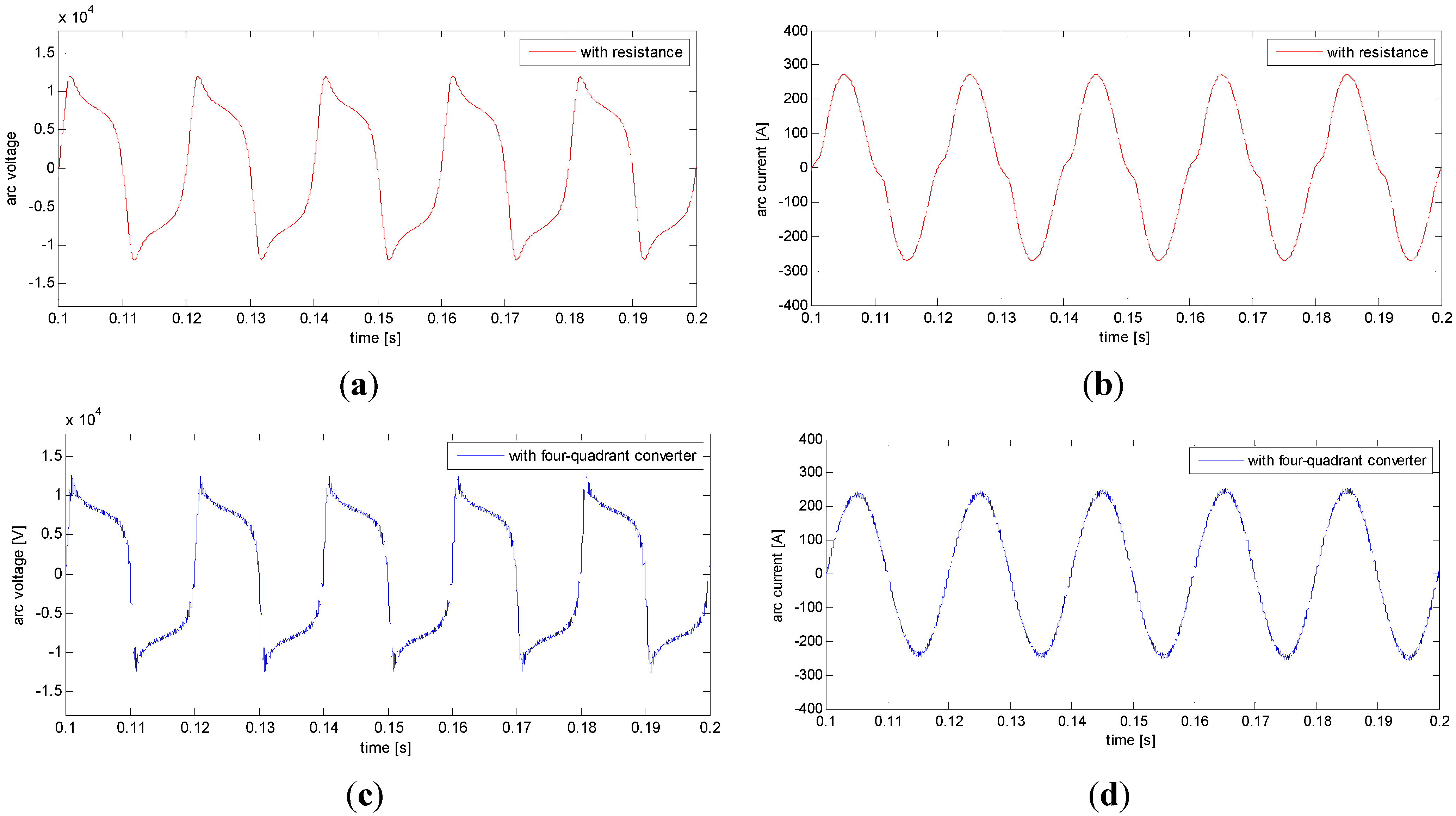
2.1.2. Pantograph Arc Model

At high speed, the electric contact becomes unreliable due to vibration, hard spots, corrosion and icing of the contact wires. Just at the beginning of a disconnection, the gap between the pantograph and catenary is small, so it is easy to break down, which causes gap discharges and arc generation. With the increasing spacing, the arc is stretched. Energy which is absorbed by the arc cannot support the arc continuing burning, so the arc will be extinguished and the pantograph separates completely from the contact wires.

The arc could last a few periods while the pantograph slides away from the contact wires [2,3,4,5]. Therefore, the arc duration time can be defined as t_arc. After the arc is extinguished, the pantograph separates from the catenary completely, the time of which can be called t_no-arc. In both mean times, the contact pressure between the pantograph and catenary is 0 N. Consequently, the disconnection-time t_loss in Table 1 is the sum of t_arc and t_no-arc. The arc-containing ratio p_arc can be expressed as p_arc = t_arc/t_loss.

The significant feature of the common black arc model is the use of the non-linear arc conductance to represent the dynamic characteristics of an arc. Generally, arc conductance is a function of the power supplied to the plasma channel, power transported by cooling, radiation and time. An ordinary differential equation form can be related to the arc voltage and arc current [22]:

$$\frac{d\ln g}{dt}=\frac{1}{\tau (u,i)}\left[\frac{ui}{P(u,i)}-1\right]$$

(4)

where g, u and i express the arc conductance, voltage and current, respectively. P(u,i) and τ(u,i) are the cooling power and time constant, respectively.

Most of the published work on arc models is based on the well-known Cassie and Mayr models [23,24,25], which provide a qualitative description of the arc in the high and low current regions, respectively. The fitting of the model results to measured data is achieved by means of a proper selection of arc parameters like the time constant and the cooling power, which is normally taken as a function of the arc current and voltage [26]. For the Mayr and Cassie arc models, Equation (4) can be expressed as follows:

$$\frac{d\ln g_m}{dt}=\frac{1}{{\tau }_m}\left[\frac{ui}{P_m}-1\right]$$

(5)

$$\frac{d\ln g_c}{dt}=\frac{1}{{\tau }_c}\left[\frac{u^2}{U_c^2}-1\right]$$

(6)

where g_m and g_c are the Mayr and Cassie arc conductance, respectively, τ_m and τ_c express the Mayr and Cassie arc time constant, respectively. P_m is the cooling power in the Mayr arc model and U_c is the static arc voltage.

Cassie’s equation shows good results for larger currents, while Mayr’s is better for the zero current section [27]. Much literature has referred to the combined Cassie and Mayr models in order to represent the dynamic arc in a wide current region [28]. Habedank had done a large amount of theoretical analysis to find a new method to describe the arc conductance using a constant. For larger currents almost all the voltage is at the Cassie part and just before the zero current section the Mayr part takes over. The arc conductance can be calculated as [29]:

$$\frac{1}{g}=\frac{1}{g_c}+\frac{1}{g_m}$$

(7)

where g_c and g_m in Equation (7) have been expressed in Equations (5) and (6).

The Habedank arc model is composed of Equations (5)–(7). Studies have shown that the combined model is suitable for a wider current application range.

Pantograph arc burning is related to the relative sliding speed between the pantograph and catenary, arc current, electrode materials and geometrical morphology [30], but these factors cannot be precisely described in Equations (5) and (6). This paper has changed P_m and U_c to get different arc waveforms for further analysis. Moreover, arc waveforms can be considered as staying the same each period during their burning time.

2.2. Traction Transformer

The traction transformer is a significant piece of energy transmission equipment between the pantograph-OCS and traction drive system. Table 2 presents the main traction transformer parameters of a train in China.

Table 2. Main traction transformer parameters.

Parameters	Primary winding	Traction winding
Capacity (kVA)	3855	1667.5
Rated voltage (V)	25000	1658
Rated current (A)	154	1006×2
Frequency (Hz)	50
Efficiency	95%

Table 2. Main traction transformer parameters.

Parameters	Primary winding	Traction winding
Capacity (kVA)	3855	1667.5
Rated voltage (V)	25000	1658
Rated current (A)	154	1006×2
Frequency (Hz)	50
Efficiency	95%

Primary and secondary winding resistances are 2.58 Ω and 0.01514 Ω, respectively. They will be 3.8390 Ω and 0.02225 Ω taking conversion to 150 °C. The no-load loss and load loss are 1103 W and 136,081 W, respectively.

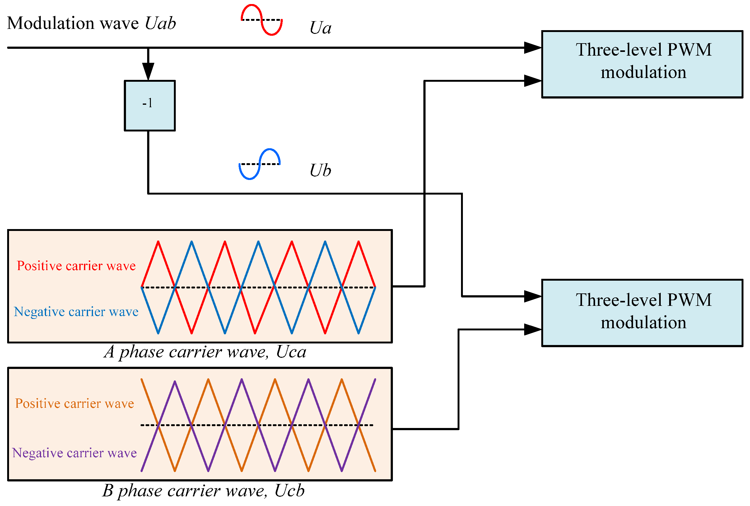
2.3. Four-Quadrant Converter

The four-quadrant converter is linked with the secondary windings of the traction transformer. It uses PWM control technology, which could improve the power factor, reduce the harmonics and power transmission losses. Even so, the traction current contains many harmonics while the traction transformer works. The four-quadrant unit is the harmonic source and the traction transformer will generate harmonic losses.

Figure 4 shows the principle diagram of a single-phase three-level four-quadrant converter. L_N and R_N are the secondary leakage inductance and leakage resistance of the traction transformer, respectively. C₁ and C₂ are DC-link capacitance.

Figure 4. Single-phase three-level four-quadrant converter.

Figure 4. Single-phase three-level four-quadrant converter.

The general principle of PWM modulation method of three-lever four-quadrant converter is shown in Figure 5. It can generate a three-level PWM signal of the a-phase bridge arm (+1, 0, −1) by comparison of the modulation wave Ua and carrier wave Uca. The phase difference between Uca and Ucb is 180°. The PWM signal of the b-phase bridge arm can be obtained in a similar way.

Figure 5. PWM modulation method.

Figure 5. PWM modulation method.

For three-level four-quadrant converter, the u_ab could be expressed as below:

$$u_{ab}=M{U}_d\cos ({\omega }_{m}t+\beta )+{\displaystyle \sum _{m=2,4,\cdots }^{\infty }{\displaystyle \sum _{n=\pm 1,\pm 3}^{\infty }\frac{2U_d}{m\pi }{J}_n(mM\pi )\sin \frac{n}{2}\pi \cos \frac{m}{2}\pi \cos (m{\omega }_{c}t+n{\omega }_{m}t+n\beta +m\alpha )}}$$

(8)

where U_d is DC voltage; ω_m and ω_c are angular frequency of input voltage and modulation wave, respectively; J_n(x) is the n order Bessel function. M and β can be expressed as below:

$$\{\begin{array}{l}M=\frac{\sqrt{2}\sqrt{U_N^4+{(P{\omega }_m{L}_N)}^2}}{U_N{U}_d}\\ \beta =\arcsin \frac{P{\omega }_m{L}_N}{\sqrt{U_N^4+{(P{\omega }_m{L}_N)}^2}}\end{array}$$

(9)

where P is the active power of four-quadrant converter.

The secondary leakage resistance R_N is quite small and its voltage can be neglected in the voltage equation. According to Kirchhoff’s law, we can obtain the following equation:

$$U_1=K(L_N\frac{d{i}_2}{dt}+u_{ab})$$

(10)

where, U₁ and i₂ express the primary voltage and secondary current of the traction transformer; K is the transformer voltage ratio.

While the current collection of the pantograph-OCS system is functioning well, the primary voltage U₁ does not contain harmonics, and the harmonic content of the traction current should meet the voltage constraints as below:

$$L_N\frac{d{i}_{2h}}{dt}=-u_{abh}$$

(11)

According to the Equations (8)–(11), every harmonic wave of the traction current can be achieved:

$$i_{2h}=-\frac{4U_d}{m\pi \cdot L_N(m{\omega }_c+n{\omega }_m)}{J}_n(mM\pi )\sin \frac{n}{2}\pi \cos \frac{m}{2}\pi \sin (m{\omega }_{c}t+n{\omega }_{m}t+n\beta +m\alpha )$$

(12)

where, i₂ and U₂ are the traction current and secondary voltage of the traction transformer, respectively.

While there is pantograph arc discharging in the circuit, Equation (10) will be expressed as:

$$U_2=\frac{U_1-U_{arc}}{K}=L_N\frac{d{i}_2}{dt}+u_{ab}$$

(13)

where, U₁ and U_arc express the primary voltage and arc voltage, respectively. U_arc can be expressed as:

$$U_{arc}=\frac{i_1}{g_{arc}}=\frac{i_2}{K\cdot g_{arc}}$$

(14)

where, i₁ and g_arc express the primary current and arc conductance, respectively.

Consequently, the harmonic content of traction current should meet the voltage constraints as below:

$$L_N\frac{{d{i}_{2h}}^{\prime }}{dt}=-u_{abh}-\frac{{i_{2h}}^{\prime }}{K^2\cdot g_{arc}}$$

(15)

According to Equations (5)–(7), the arc conductance is related to the traction current, which leads to a more complicated analytical solution calculation of Equation (15), so we could analyze the harmonic content variations caused by the pantograph arc based on simulation results.

3. Harmonic Loss of Transformer

Commonly used formulas for harmonic core loss calculation usually need to consider nonlinearity of the core material, phase differenced and the frequency of every harmonic, the penetration depth of the corresponding wire, etc, which their calculation and application inconvenient. The traditional T-equivalent circuit model could not accurately reflect transformer parameter changes with harmonics, so an advanced T-equivalent model [18], considering the change of winding resistance and excitation resistance with harmonic frequency, has been set up in this paper. This method is simply and effective and could be programmed easily.

In Figure 6, R_h1, R_h2 and R_hm express the primary winding resistance, secondary resistance and excitation in the h-order harmonic, respectively; L_h1, L_h2 and L_hm express the primary inductance, secondary inductance and excitation inductance in the h-order harmonic, respectively; i_h1, i_h2 and i_hm are the harmonic content of the primary, secondary and excitation currents, respectively, and i_h1, i_h2 can be calculated using Equation (16); u₂(t) is the harmonic source which is produced by the four-quadrant converter. At different harmonic frequencies, the resistance is different, so the harmonic copper loss can be defined as:

$$P_{cuh}={\displaystyle \sum _{h=1}^m{R}_{h1}{I}_{h1}^2}+{\displaystyle \sum _{h=1}^m{R}_{h2}{I}_{h2}^2}$$

(16)

where P_cuh is winding loss under a harmonic environment; h is the harmonic order; R_h1 and R_h2 are the primary and secondary winding resistance in the h-order harmonic, respectively; I_h1 and I_h2 are valid values of the primary and secondary harmonic current.

Figure 6. Advanced T equivalent circuit under harmonic conditions.

Figure 6. Advanced T equivalent circuit under harmonic conditions.

In a similar way, the harmonic core loss can be approximately regarded as the excitation resistance loss, which will avoid considering the nonlinearity of the core material and complex electromagnetic field calculations. The harmonic core loss can be expressed as:

$$P_{coreh}={\displaystyle \sum _{h=1}^n{R}_{hm}{I}_{hm}^2}$$

(17)

where P_coreh is core loss under the harmonic environment; R_hm and I_hm express the excitation resistance and excitation current in the h-order harmonic, respectively.

The h-order resistance R_h1, R_h2 and R_hm can phenomenologically be approximated as below:

$$K_{h1}=R_{h1}/R_{b1}=a_0{e}^{a_{1}f}$$

(18)

$$K_{h2}=R_{h2}/R_{b2}=b_0{e}^{b_{1}f}$$

(19)

$$K_{hm}=R_{hm}/R_{bm}=c_0+c_1\times {10}^{-2}f+c_2\times {10}^{-5}{f}^2$$

(20)

where K_h1, K_h2 and K_hm express the winding resistance coefficient and excitation resistance coefficient, respectively; R_b1, R_b2 and R_bm express the winding resistance and excitation resistance at the fundamental frequency of 50 Hz. a, b and c are related coefficients and can be obtained by finite element analysis or experiments [18].

According to Equations (18)–(20), the coefficients K_h1, K_h2 and K_hm can be fitted in Figure 7. This paper has only considered orders up to the 13th. The rising slope of winding resistance coefficient is relatively smaller and the 13th harmonic coefficient is 1.37. The excitation resistance coefficient reaches 3.932 in the 13th harmonic.

Figure 7. Change of coefficient with frequency.

Figure 7. Change of coefficient with frequency.

In [31,32] the advanced T-equivalent circuit method in Figure 6 was compared with an experimental measurement method. Results have demonstrated they can be consistent with each other within a certain error range, so the advanced method can be applied to the harmonic loss calculation of traction transformers. This method does not involve complicated nonlinear parameters, and is easy to realize using MATLAB programming. Calculation parameters can be obtained by basic transformer experiments. Consequently, this method can be used for predicting the harmonic losses when the harmonic components are known.

4. Results and Discussion

4.1. Harmonic Loss Calculation

Arc voltage and current while the traction windings of the traction transformer are connecting with the resistance load are shown in Figure 8a,b. Figure 8c,d presents the arc voltage and current while two traction windings are connecting with two four-quadrant converters, respectively.

Figure 8. (a) Arc voltage with resistance load; (b) Arc current with resistance load; (c) Arc voltage with four-quadrant converter load; and (d) Arc current with four-quadrant converter load.

Figure 8. (a) Arc voltage with resistance load; (b) Arc current with resistance load; (c) Arc voltage with four-quadrant converter load; and (d) Arc current with four-quadrant converter load.

Three features could be found in the Figure 8a,b. Firstly, the arc current obviously presents a zero section. Secondly, the distortion of the arc voltage and current is serious, and the nonlinear variation of the arc manifests that it has produced high-frequency components. Thirdly, the arc voltage waveform presents transients at the moment of arc starting. Figure 8c manifests many ripples based on Figure 8a by contrast with the arc voltage waveforms. The zero-current section of the arc has disappeared and produced high-frequency components because of the four-quadrant converter. Arc features will be different due to variations of the arc parameters presented in Equations (5)–(7).

The equivalent interfering current is an important standard to analyze the characteristic harmonics in the traction calculations of electric locomotives, so we want to analyze the effects on the equivalent interfering current caused by the pantograph arc. We also want to analyze the relationships between equivalent interfering current and harmonic losses. The equivalent interfering current can be expressed as below:

$$I_p=\sqrt{{\displaystyle \sum _{h=1}^{\infty }{I}_h^2{\omega }_h^2}}$$

(21)

where I_p and I_h are the equivalent interfering current and h-order harmonic current, respectively; ω_h is the equivalent interfering weighting coefficient. It has been defined in the International Telegraph and Telephone Consultative Committee (CCITT).

We have obtained primary voltage and primary current waveforms while there is arc discharging in the circuit and there is no arc (see Figure 9 and Figure 10) to analyze the effects on harmonic current, equivalent interfering current and harmonic losses caused by pantograph arcs. The blue curves and red curves express the with-arc and without-arc results in the circuit, respectively.

In Figure 9, while the pantograph arc model is discharging in the circuit, its partial-voltage effect will lead to a decreasing primary voltage amplitude, and distortion near the zero crossing point at the same time. Odd harmonics will increase sharply while there is arc in the circuit. The excitation current is approximately proportional to the primary voltage. The equivalent interfering current of the excitation winding is 4.19 × 10⁻⁴ with arc and 1.4768 × 10⁻⁵ without arc, respectively.

Figure 9. Primary voltage of the traction transformer.

Figure 9. Primary voltage of the traction transformer.

In Figure 10, due to the constant power control of the four-quadrant converter, the decreasing amplitude of the primary voltage will lead to an increasing amplitude primary current. The equivalent interfering current of the primary windings is 0.51338 with arc and 0.49753 without arc, and the equivalent interfering current of the secondary windings is 3.892264 and 3.73168, respectively. Because the harmonic contents of the primary and secondary current do not change too much with-arc and without-arc in the circuit, the equivalent interfering currents of the primary and secondary windings do not have evident differences.

Figure 10. Primary current of the traction transformer.

Figure 10. Primary current of the traction transformer.

Harmonic copper loss and harmonic core loss are affected by the harmonic current and harmonic voltage, respectively. They can be calculated by Equations (16) and (17). We have defined the relative loss to express variations of the harmonic loss:

$$P_r=\frac{P_{arc}}{P_{no-arc}}$$

(22)

where, P_r is the relative harmonic loss; P_arc and P_no-arc express the harmonic loss while there is arc and no arc discharging in the circuit. Consequently, P_r expresses that the multiples of P_arc to P_no-arc.

Figure 11 presents the primary and secondary equivalent interfering current variations caused by different pantograph arc voltages. Figure 12 presents the relative harmonic copper loss which was defined in Equation (22).

Figure 11. (a) Primary equivalent interfering current and (b) Secondary equivalent interfering current.

Figure 11. (a) Primary equivalent interfering current and (b) Secondary equivalent interfering current.

Figure 12. (a) Primary relative harmonic copper loss and (b) Secondary relative harmonic copper loss.

Figure 12. (a) Primary relative harmonic copper loss and (b) Secondary relative harmonic copper loss.

In Figure 11 and Figure 12, because the excitation current is negligible compared to the primary and secondary currents, the variations trend of the equivalent interfering current and harmonic copper loss of the primary windings and secondary windings stay nearly the same. With the increasing pantograph arc voltage, the primary and secondary equivalent interfering current are not always rising, and sometimes the equivalent interfering current with arc is less than that without arc. This is because arc discharging may lead to h-order harmonics increasing or decreasing sometimes. In Figure 11, even though the harmonic contents of the primary and secondary current are decreasing a lot at point A, which has made the equivalent interfering current at this point the least, the harmonic copper loss is not the least at this point. On the contrary, odd and even harmonic contents are increasing a lot at point B, which has caused a raise of the equivalent interfering current. Results in Figure 11 have shown that the pantograph arc does not always improve the primary and secondary harmonic current content. Although the equivalent interfering variations are irregular, harmonic copper losses are still greater than those without arcs in the circuit. In other words, arc discharging in the circuit will increase harmonic copper loss. In general, their variations have shown an increasing trend. The harmonic copper loss with arcs in the circuit can reach almost two times that without arcs. In combination with the results of Figure 11 and Figure 12, the relationship between equivalent interfering current and harmonic copper loss is disproportionate and irregular, so we could not estimate the harmonic copper loss according to variations of arc voltage and equivalent interfering current.

Figure 13a,b presents the excitation equivalent interfering current and relative harmonic core loss variations. Variations of harmonic core loss with the increasing arc voltage are smooth and regular. This is because the zero-cross distortion of the primary voltage (see blue curve in Figure 9) will be worse with the rising arc voltage. Therefore, the harmonic components of the primary voltage are increasing regularly. Similarly, the h-order harmonic content of the excitation current is increasing sharply with the rising arc voltage.

Figure 13. (a) Excitation equivalent interfering current and (b) Relative harmonic core loss.

Figure 13. (a) Excitation equivalent interfering current and (b) Relative harmonic core loss.

In Figure 13a, the excitation equivalent interfering current variations are proportional to the arc voltage. In Figure 13b, while there is no arc discharging in the circuit, the harmonic content of the excitation current is too small to generate any harmonic core loss. The relative harmonic core loss is growing exponentially with the sharply increasing h-order harmonic content of the excitation current. This has led to the harmonic core loss becoming a few hundred times that without arc. Moreover, we can obtain a regular relationship between the excitation equivalent interfering current and the harmonic core loss (not shown), whose trend is approximately same as that seen in Figure 13b. Harmonic core losses can be estimated according to the variations of the excitation equivalent interfering current if it is known.

In brief, while there is relatively stable arc burning in the circuit, we can calculate the transformer loss variations accurately using Equations (16) and (17) when the harmonic current is known. Moreover, we can also estimate the harmonic losses according to the variation trend of Figure 12b and Figure 13b. These methods can be programmed easily and used in the loss calculation and in estimating the normal or abnormal operating state of the high-speed train.

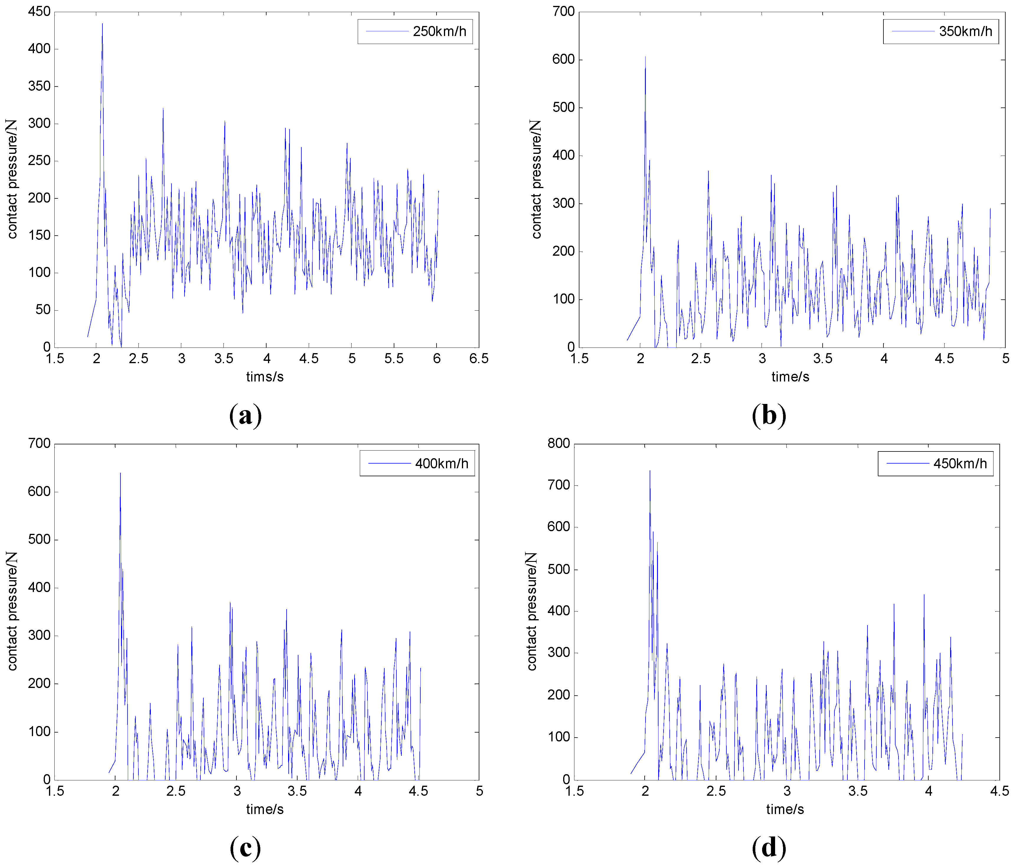
4.2. Effects of Disconnection Events

In order to analyse the relations between disconnection events and traction transformer loss, this paper has defined average loss and p_arc, which express the arc containing ratio in the disconnection time t_loss. Therefore the average copper loss P_copper(avg) can be defined by Equation (23):

$$P_{copper}(avg)=\frac{P_{copper}(no-arc)\times t_{contact}+P_{copper}(arc)\times t_{loss}\times p_{arc}}{t_{total}}$$

(23)

In a similar way, the average core loss can be expressed by Equation (24):

$$P_{core}(avg)=\frac{P_{core}(no-arc)\times t_{contact}+P_{core}(arc)\times t_{loss}\times p_{arc}}{t_{total}}$$

(24)

where P_copper(avg) and P_core(avg) express the relative harmonic copper loss and relative harmonic core loss, respectively.

Take a speed of 450 km/h as an example (see Table 1), the total simulation time t_total is 2.34 s, and disconnection time t_loss and contact time t_contact are 0.67 s and 1.67 s, respectively (see Table 1). Supposing the arc containing ratio is 30%, this indicates that the total arc duration time is 0.67 × 30% = 0.201 s, instead, the complete disconnection time without arc is 0.67 × (1%−30%) = 0.469 s. The average copper loss can be calculated by [P_copper(no-arc) × 1.67 s + P_copper(arc) × 0.201 s]/2.34 s.

Figure 14 shows the variations of average P_copper(avg) and P_core(avg) with the rising arc containing ratio p_arc when the arc voltage is 6000 V. P_copper(avg) and P_core(avg) are proportionally growing by horizontal comparison because of the linearly increasing arc containing ratio, however, the growth slope is increasing with the rising speed.

Figure 14. (a) Relative harmonic copper loss with different disconnection ratios. And (b) relative harmonic core loss with different disconnection ratios.

Figure 14. (a) Relative harmonic copper loss with different disconnection ratios. And (b) relative harmonic core loss with different disconnection ratios.

In Figure 14a, the average harmonic copper loss almost does not change at the speed of 250 km/h. Instead, variations of P_copper(avg) are obvious while p_arc is growing from 10% to 100% at the speed of 450 km/h. Then, while the harmonic copper loss is less than that without arc, P_copper(avg) is decreasing with the rising disconnection ratio by longitudinal comparison. On the contrary, P_copper(avg) is increasing with the rising disconnection ratio while the harmonic copper loss is greater than that without arc. In Figure 14b, the average harmonic core loss is increasing with the rising arc containing ratio by horizontal comparison, and increasing with the rising disconnection ratio by longitudinal comparison.

Figure 15 shows the variations of average harmonic loss P_copper(avg) and P_core(avg) with the rising arc containing ratio at the speed of 350 km/h. In Figure 15a, P_copper(avg) is growing with the increasing arc voltage at a constant p_arc by longitudinal comparison. The growth slope of P_copper(avg) also rises with the growing arc resistive state. The horizontal comparison results are the same as in Figure 14a. Results in Figure 15b are the same as those in Figure 14b by horizontal comparison, and the average harmonic core loss is increasing with the rising disconnection ratio by longitudinal comparison.

Figure 15. (a) Relative harmonic copper losses with different arc voltages and (b) Relative harmonic core losses with different arc voltages.

Figure 15. (a) Relative harmonic copper losses with different arc voltages and (b) Relative harmonic core losses with different arc voltages.

The results above indicate that the pantograph-OCS electrical contact properties will affect the traction transformer loss. These parameters include pantograph arc voltage and disconnection ratio at different speeds. According to Figure 11, Figure 12 and Figure 13, if an operating state of a high-speed train in a route is known, we can estimate the additional energy consumption of the traction transformer caused by pantograph arcs.

High-speed trains run at almost 200 km/h~350 km/h at present, but the train speed will improve in the future; more frequent disconnection ratios and more arc burning will increase the additional energy consumption. Consequently, the traction transformer energy consumption needs to be considered in the high-speed train operation now and in the future.

5. Conclusions

This paper is proposed based on a harmonic T-equivalent circuit model, considering the pantograph arcs in a poor current collection situation and disconnection events of the pantograph-OCS, and analyzes the effects on the traction transformer harmonic losses. We can draw the following conclusions:

(1)

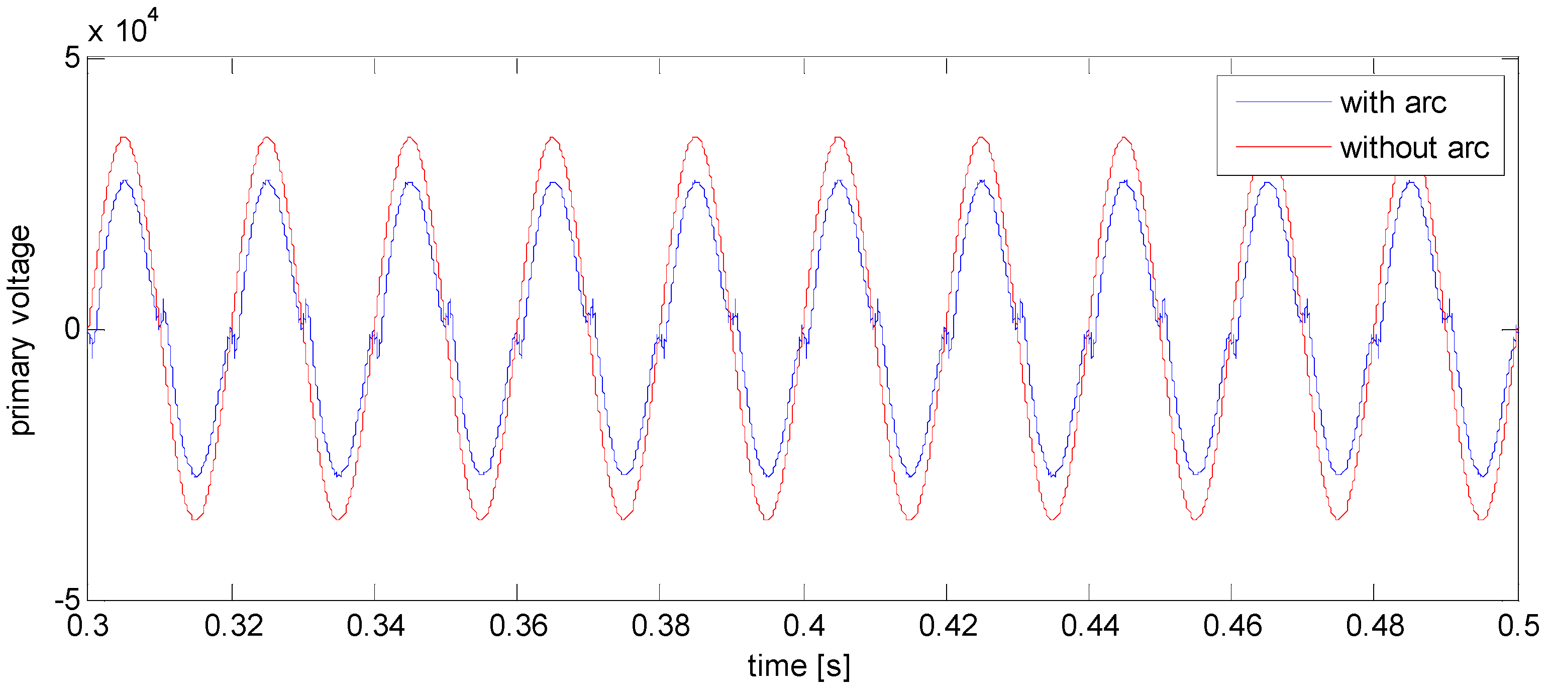
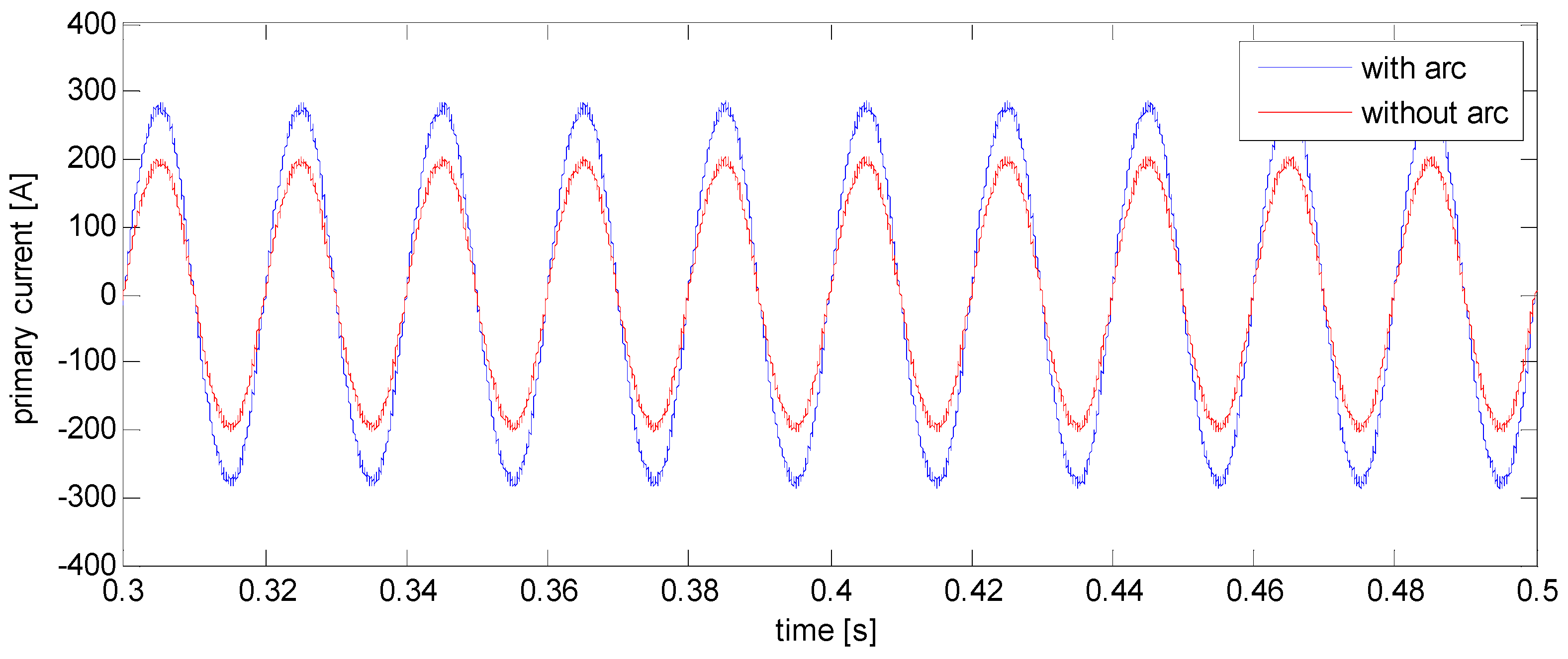
The increasing pantograph arc voltage leads to decreasing primary voltage and increasing primary current; this will lead to both increasing harmonic copper losses and harmonic core losses.

(2)

The effects of pantograph arcs on the primary and secondary equivalent interfering current are irregular, but the excitation equivalent interfering current is increasing with the rising arc voltage.

(3)

The harmonic copper loss with arc in the circuit can reach almost two times that without arc. The harmonic core loss with arc is increased significantly compared with that without arc.

(4)

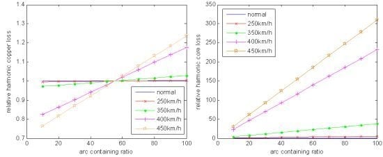
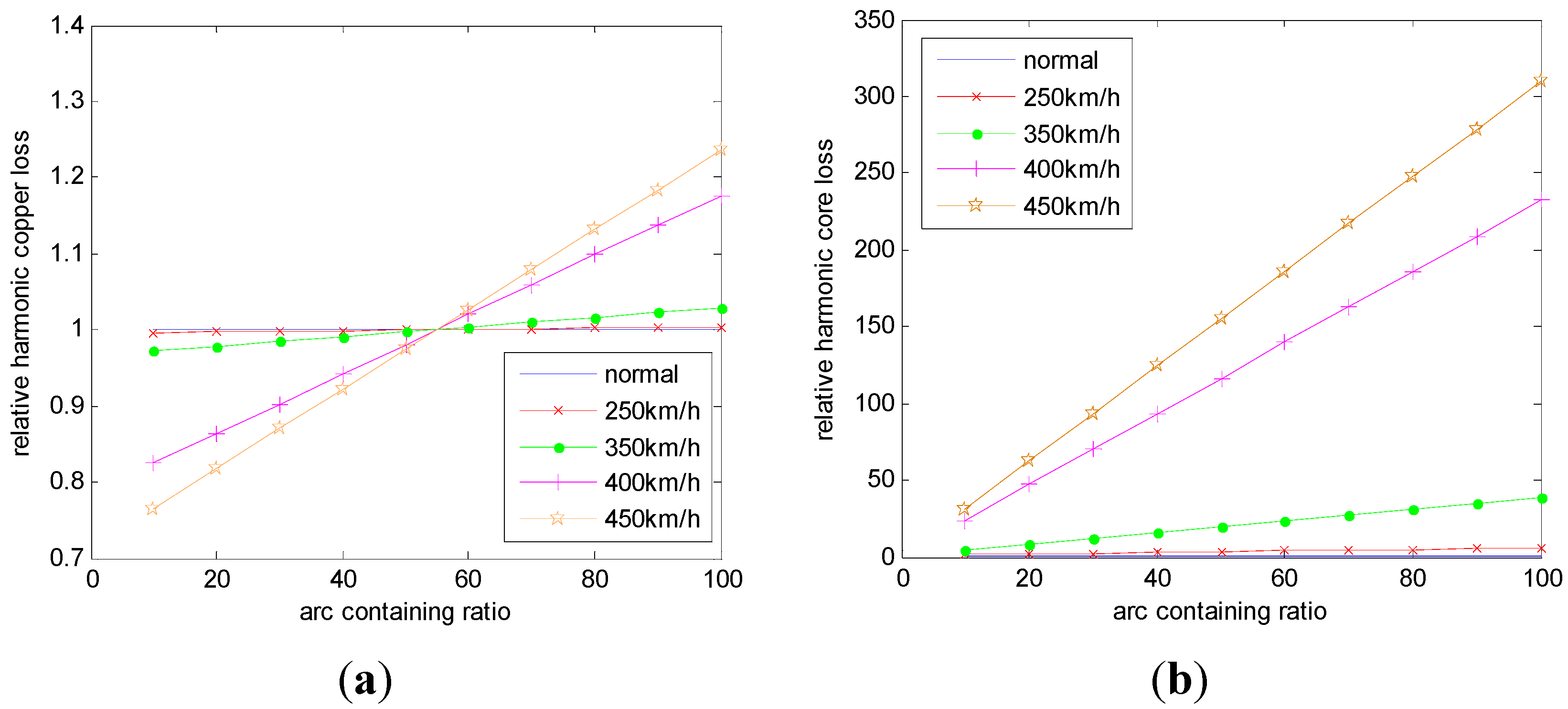
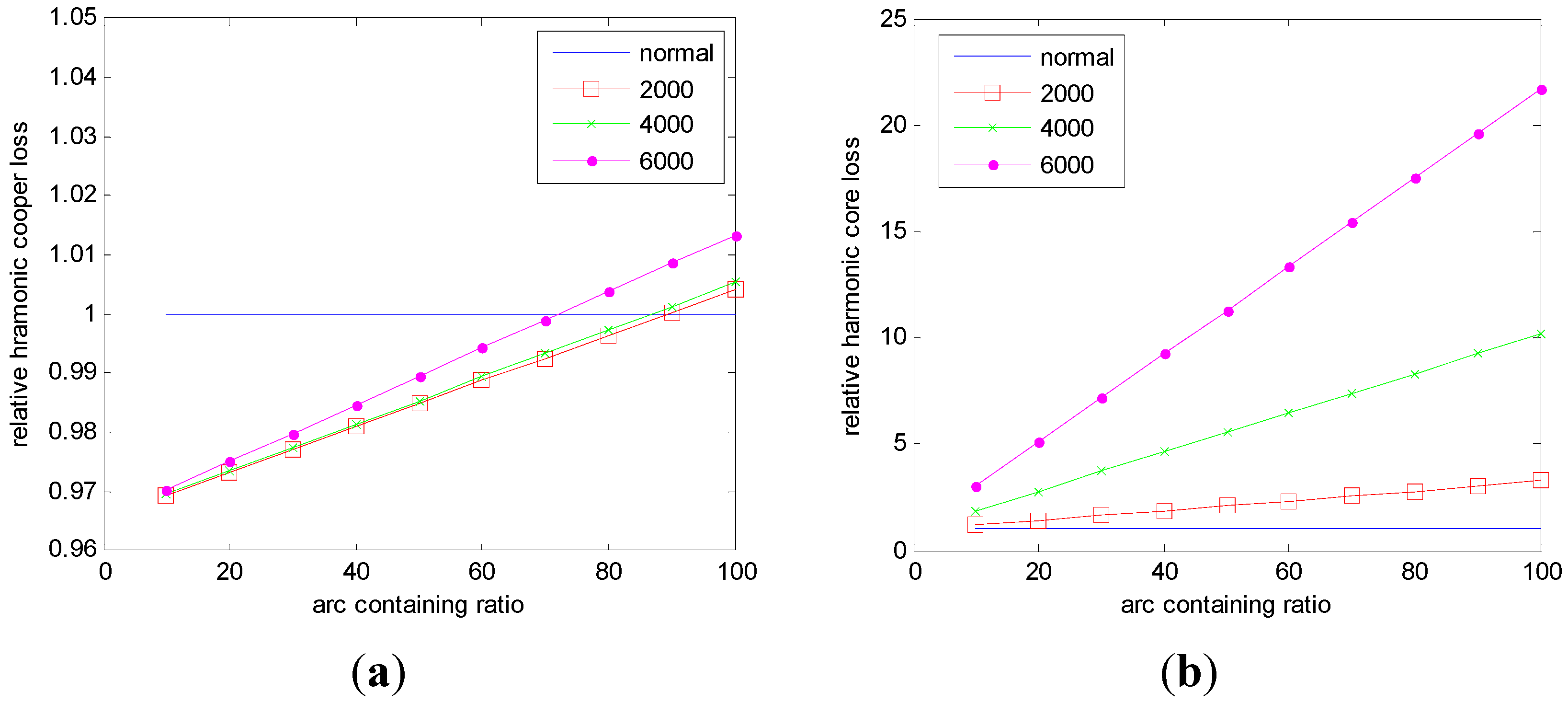
The average harmonic loss is rising with the growing arc containing ratio and the rising arc voltage. The average harmonic copper loss may be less than that without arc while the arc containing ratio is small. The average harmonic core loss is always larger than that without arc.

The results above provide a data reference to reduce the loss variations and judge the operation of the equipment under different electrical contact properties conditions of a pantograph-OCS. Therefore the traction transformer harmonic losses can be predicted if the harmonic components have been known. It could also be estimated using arc voltage variations. Although the harmonic losses are changing with the pantograph arcs, they account for the fact the increasing fundamental losses are still relatively small. However, the harm of harmonic contents which will cause noise, mechanical vibration and even mechanical resonance cannot be ignored. Increasing harmonic losses will lead to local overheating, additional energy consumption, declining efficiency and decreasing equipment lifetimes. On the other hand, the inhibition of pantograph arcs by controlling the power factors of the four-quadrant converter is significant and the effects of unbalanced loads will be considered in future research.

References

1. China South Locomotive and Rolling Stock Corporation Limited Web Page. High-speed EMU of CRH380A. 16 March 2011. Available online: http://www.csrgc.com.cn/cns/cpyfw/dcz/2011-03-16/3921.shtml (accessed on 31 October 2013).
2. Bormann, D.; Midya, S.; Thottappillil, R. DC Component in Pantograph Arcing: Mechanisms and Influence of Various Parameters. In Proceedings of the 18th International Zurich Symposium on Electromagnetic Compatibility (EMC Zurich 2007), Munich, Germany, 24–28 September 2007; pp. 369–372.
3. Midya, S.; Bormann, D.; Schutte, T.; Thottappillil, R. Pantograph arcing in electrified railways—Mechanism and influence of various parameters—Part I: With DC traction power supply. IEEE Trans. Power Deliv. 2009, 24, 1931–1939. [Google Scholar] [CrossRef]
4. Midya, S.; Bormann, D.; Schutte, T.; Thottappillil, R. Pantograph arcing in electrified railways—Mechanism and influence of various parameters—Part II: With AC traction power supply. IEEE Trans. Power Deliv. 2009, 24, 1940–1950. [Google Scholar] [CrossRef]
5. Midya, S.; Bormann, D.; Schutte, T.; Thottappillil, R. DC component from pantograph arcing in AC traction system—Influencing parameters, impact, and mitigation techniques. IEEE Trans. Electromagn. Compat. 2011, 53, 18–27. [Google Scholar] [CrossRef]
6. Mayuri, R.; Sinnou, N.R.; Ilango, K. Eddy Current Loss Modeling in Transformer Iron Losses Operated by PWM Inverter. In Proceedings of the 2010 Joint International Conference on Power Electronics, Drives and Energy Systems (PEDES) & 2010 Power India, New Delhi, India, 20–23 December 2010; pp. 1–5.
7. Liu, R.; Mi, C.C.; Gao, D.W. Modeling of eddy-current loss of electrical machines and transformers operated by pulsewidth-modulated inverters. IEEE Trans. Magn. 2008, 44, 2021–2028. [Google Scholar] [CrossRef]
8. Yazdani-Asrami, M.; Mirzaie, M.; Akmal, A.A.S. Investigation on Impact of Current Harmonic Contents on the Distribution Transformer Losses and Remaining Life. In Proceedings of the 2010 IEEE International Conference on Power and Energy (PECon), Kuala Lumpur, Malaysia, 29 November–1 December 2010; pp. 689–694.
9. Forrest, J.A.C. Harmonic load losses in HVDC converter transformers. IEEE Trans. Power Deliv. 1991, 6, 153–157. [Google Scholar] [CrossRef]
10. Soualmi, A.; Dubas, F.; Depernet, D.; Randria, A.; Espanet, C. Study of Copper Losses in the Stator Windings and PM Eddy-Current Losses for PM Synchronous Machines Taking into Account Influence of PWM Harmonics. In Proceedings of the 2012 15th International Conference on Electrical Machines and Systems (ICEMS), Sapporo, Japan, 21–24 October 2012; pp. 1–5.
11. Fu, R.; Dou, M. Research on Rotor Harmonic Copper Losses of Line-start REPMSM Based on FEM. In Proceedings of the 2008 International Conference on Electrical Machines and Systems (ICEMS 2008), Wuhan, China, 17–20 October 2008; pp. 3085–3089.
12. Elmoudi, A.; Lehtonen, M.; Nordman, H. Corrected Winding Eddy-Current Harmonic Loss Factor for Transformers Subject to Nonsinusoidal Load Currents. In Proceedings of the 2005 IEEE Russia Conference on Power Tech, St. Petersburg, Russia, 27–30 June 2005; pp. 1–6.
13. Ma, X.J.; Jiang, Y. Study on Eddy Current Loss of Core Tie-Plate in Power Transformers. In Proceedings of the 2010 Asia-Pacific Power and Energy Engineering Conference (APPEEC), Chengdu, China, 28–31 March 2010.
14. Milagre, A.M.; Ferreira da Luz, M.V.; Cangane, G.M.; Komar, A.; Avelino, P.A. 3D Calculation and Modeling of Eddy Current Losses in a Large Power Transformer. In Proceedings of the 2012 20th International Conference on Electrical Machines (ICEM), Marseille, France, 2–5 September 2012; pp. 2282–2286.
15. Li, Y.; Eerhemubayaer.; Sun, X.; Jing, Y.T.; Li, J. Calculation and Analysis of 3-D Nonlinear Eddy Current Field and Structure Losses in Transformer. In Proceedings of the 2011 International Conference on Electrical Machines and Systems (ICEMS), Beijing, China, 20–23 August 2011; pp. 1–4.
16. Zhang, Y.; Yan, B.; Cao, F.; Xie, D.; Zeng, L. Analysis of Eddy Current Loss and Local Overheating in Oil Tank of a Large Transformer Using 3-D FEM. In Proceedings of the 2011 International Conference on Electrical Machines and Systems (ICEMS), Beijing, China, 20–23 August 2011; pp. 1–4.
17. Da luz, M.V.F.; Leite, J.V.; Benabou, A.; Sadowski, N. Three-phase transformer modeling using a vector hysteresis model and including the eddy current and the anomalous losses. IEEE Trans. Magn. 2010, 46, 3201–3204. [Google Scholar] [CrossRef]
18. Makram, E.B.; Thompson, R.L.; Girgis, A.A. A new laboratory experiment for transformer modeling in the presence of harmonic distortion using a computer controlled harmonic generator. IEEE Trans. Power Syst. 1988, 3, 1857–1863. [Google Scholar] [CrossRef]
19. Park, T.J.; Han, C.S.; Jang, J.H. Dynamic sensitivity analysis for pantograph of a high-speed rail vehicle. J. Sound Vib. 2003, 266, 235–260. [Google Scholar] [CrossRef]
20. Zhou, N.; Zhang, W. Investigation on dynamic performance and parameter optimization design of pantograph and catenary system. Finite Elem. Anal. Des. 2011, 47, 288–295. [Google Scholar] [CrossRef]
21. Cho, Y.H.; Lee, K.; Park, Y.; Kang, B.; Kim, K.N. Influence of contact wire pre-sag on the dynamics of pantograph-railway catenary. Int. J. Mech. Sci. 2010, 52, 1471–1490. [Google Scholar] [CrossRef]
22. Guardado, J.L.; Maximov, S.G.; Melgoza, E.; Naredo, J.L.; Moreno, P. An improved arc model before current zero based on the combined Mayr and Cassie arc models. IEEE Trans. Power Deliv. 2005, 20, 138–142. [Google Scholar] [CrossRef]
23. Liu, Y.J.; Chang, G.W.; Huang, H.M. Mayr’s equation-based model for pantograph arc of high-speed railway traction system. IEEE Trans. Power Deliv. 2010, 25, 2025–2027. [Google Scholar] [CrossRef]
24. Wu, X.X.; Li, Z.B.; Tian, Y.; Mao, W.J.; Xie, X. Investigate on the Simulation of Black-Box Arc Model. In Proceedings of the 2011 1st International Conference on Electric Power Equipment—Switching Technology (ICEPE-ST), Xi’an, China, 23–27 October 2011; pp. 629–636.
25. Bizjak, G.; Zunko, P.; Povh, D. Circuit breaker model for digital simulation based on Mayr’s and Cassie’s differential arc equations. IEEE Trans. Power Deliv. 1995, 10, 1310–1315. [Google Scholar] [CrossRef]
26. Habedank, U. On the mathematical description of arc behavior in the vicinity of current zero. EtzArchiv Elektrotech. Bd 1988, 10, 339–343. [Google Scholar]
27. Parizad, A.; Baghaee, H.R.; Tavakoli, A.; Jamali, S. Optimization of Arc Models Parameters Using Genetic Algorithm. In Proceedings of the 2009 International Conference on Electric Power and Energy Conversion Systems (EPECS’09), Sharjah, United Arab Emirates, 10–12 November 2009; pp. 1–7.
28. Tseng, K.J.; Wang, Y.M.; Vilathgamuwa, D.M. An experimentally verified hybrid Cassie-Mayr electric arc model for power electronics simulations. IEEE Trans. Power Electron. 1997, 12, 429–436. [Google Scholar] [CrossRef]
29. Habedank, U. Improved Evaluation of Short-Circuit Breaking Tests. In Proceedings of the Conseil International Des Grands Reseaux Elecctriques, Colloquium of CIGRE SC 13, Sarajevo, Yugoslavia, May 1989.
30. Demetrios, K.; Reuben, H.; Frank, A.B. Magnetically controlled arcs for power collection. IEEE Trans. Ind. Appl. 1981, IA-17, 174–178. [Google Scholar]
31. Li, P.; Li, G.; Xu, Y.; Yao, S. Methods Comparation and Simulation of Transformer Harmonic Losses. In Proceedings of the 2010 Asia-Pacific Power and Energy Engineering Conference (APPEEC), Chengdu, China, 28–31 March 2010.
32. Zhang, B.; Liu, Y.; Zhao, K.; Jiang, C.; Zhang, Z.L. Transformer Loss Calculation and Analysis Driven by Load Harmonics. In Proceedings of the 2011 International Conference on Electrical and Control Engineering (ICECE), Yichang, China, 16–18 September 2011; pp. 1394–1398.