Nonlinear Power-Level Control of the MHTGR Only with the Feedback Loop of Helium Temperature

Abstract

Power-level control is a crucial technique for the safe, stable and efficient operation of modular high temperature gas-cooled nuclear reactors (MHTGRs), which have strong inherent safety features and high outlet temperatures. The current power-level controllers of the MHTGRs need measurements of both the nuclear power and the helium temperature, which cannot provide satisfactory control performance and can even induce large oscillations when the neutron sensors are in error. In order to improve the fault tolerance of the control system, it is important to develop a power-level control strategy that only requires the helium temperature. The basis for developing this kind of control law is to give a state-observer of the MHTGR a relationship that only needs the measurement of helium temperature. With this in mind, a novel nonlinear state observer which only needs the measurement of helium temperature is proposed. This observer is globally convergent if there is no disturbance, and has the L₂ disturbance attenuation performance if the disturbance is nonzero. The separation principle of this observer is also proven, which denotes that this observer can recover the performance of both globally asymptotic stabilizers and L₂ disturbance attenuators. Then, a new dynamic output feedback power-level control strategy is established, which is composed of this observer and the well-built static state-feedback power-level control based upon iterative dissipation assignment (IDA-PLC). Finally, numerical simulation results show the high performance and feasibility of this newly-built dynamic output feedback power-level controller.

1. Introduction

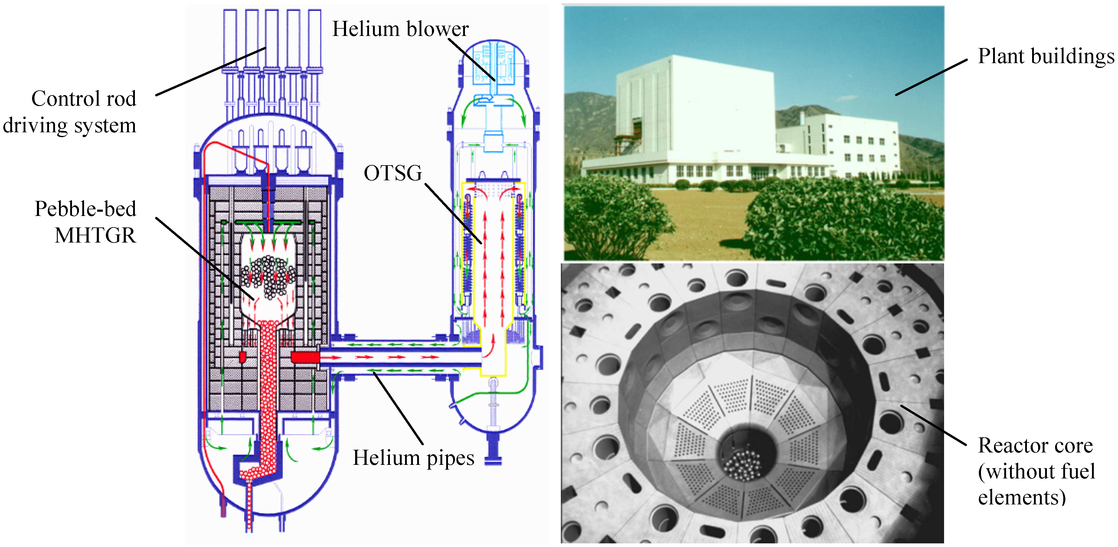
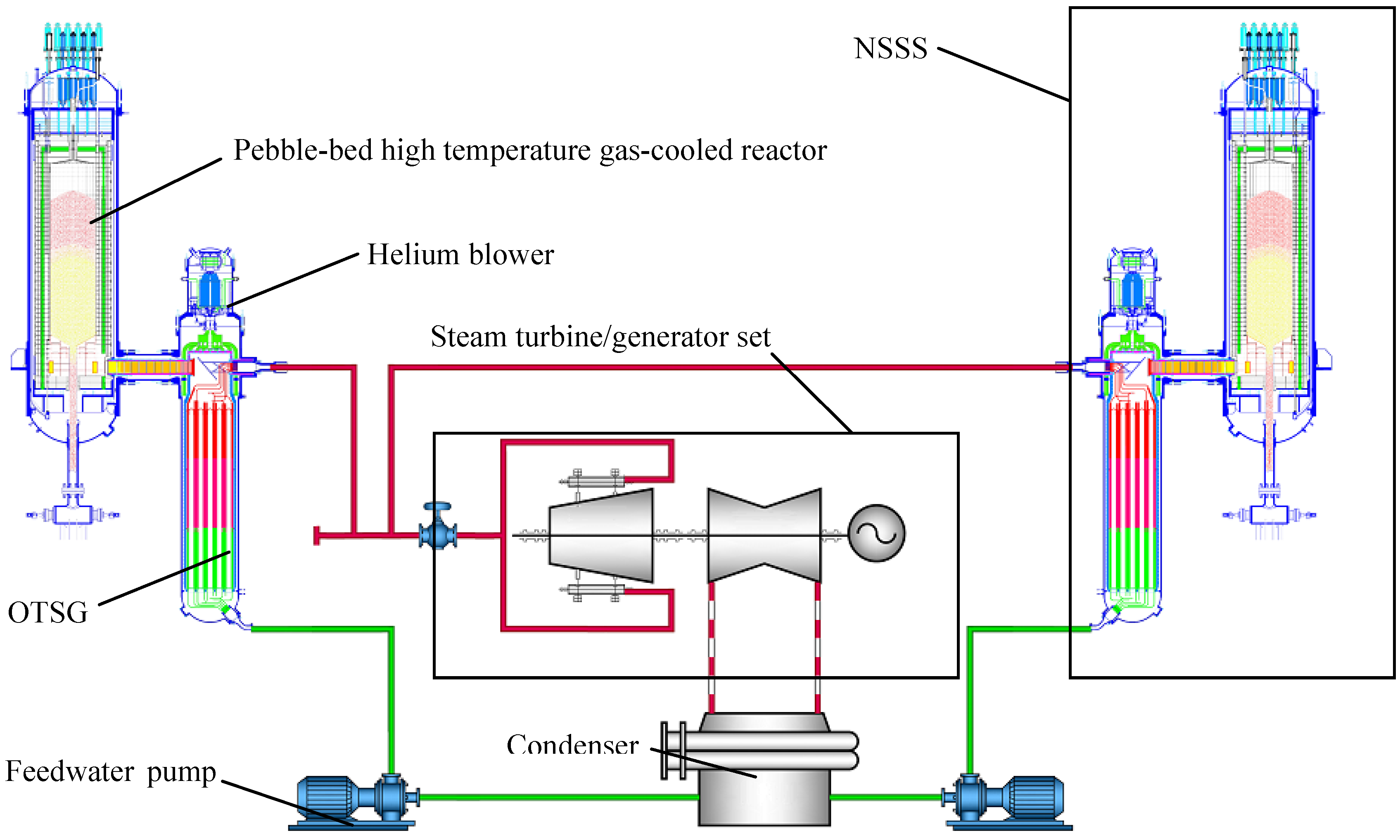
Although there have been some severe accidents, i.e., Three Mile Island, Chernobyl and Fukushima, nuclear energy is still the sole energy source that can substitute for fossil fuels in a centralized way and in a great amount with commercial availability and economic competitiveness. These accidents should not hinder the renaissance of nuclear energy, and they can stimulate the nuclear energy community to develop more safety, reliable and efficient nuclear power plants. It is well known that modular high temperature gas-cooled reactors (MHTGRs, such as the HTR-Module designed in Germany and the MHTGR designed in the US), which have inherent safety features and market flexibility, are candidates for the next generation of nuclear power plants. MHTGRs use helium as coolant and graphite as both moderator and structural material, and its fuel elements contain thousands of very small coated particles that are embedded in a graphite matrix. The coatings surrounding the particle kernel produce a robust energy source by acting as the containment boundary for the encapsulated material. There are two kinds of fuel elements for the MHTGR design, i.e., spherical and the prismatic elements. The former are exemplified by pebble-bed cores such as those in the AVR, THTR-300 and HTR-Module, and the latter leads to cylindrical cores such as Peach-Bottom and Fort. St. Vrain. The development of the MHTGR in China is inspiring. Supported by the Chinese national high-technology program, a 10 MW_th high temperature gas-cooled test reactor (HTR-10) reached criticality and full power generation in December 2000 and January 2003, respectively [1]. Five safety experiments were then carried out on the HTR-10 in October 2003, which verified and demonstrated many inherent safety features of the MHTGR design [2]. A schematic view of the HTR-10 unit is shown in Figure 1. Based upon the experience in design and construction of the HTR-10, the high temperature gas-cooled reactor pebble-bed module (HTR-PM) project is then proposed. The major target of this project is to build a pebble-bed MHTGR demonstration plant which consists of two pebble-bed one-zone module reactors of combined 2 × 250 MW_th power, and adopts the operation scheme of two modules connected to one steam turbine/generator set [3,4]. Figure 2 shows that the module here is just a nuclear steam supplying system (NSSS) which is composed of an MHTGR, a helical coiled once-through steam generator (OTSG) and the necessary connecting pipes.

Power-level regulation is a significant technique guaranteeing the safe, stable and efficient operation of all types of nuclear reactors. Due to the wide development of pressurized water reactors (PWRs), there have been some strong results in the field of power-level control for the PWRs. Edwards et al. developed the state feedback assisted classical controller (SFAC) which utilizes the state-feedback to modify the demand signal for an embedded classical output feedback controller, and is useful for existing power plant implementation since it leaves the current classical feedback loop in place [5]. In order to strengthen the robustness of the SFAC, a linear quadratic Gaussian regulation with loop transfer recovery (LQG/LTR) technique is then applied under the SFAC configuration [6,7]. A diagonal recurrent neural network was also applied for the improvement of temperature regulation performance [8]. These power-level control laws require a measurement of the nuclear power and provide regulation of both the nuclear power and coolant temperature. Moreover, there are some other types of advanced power-level control for nuclear reactors such as the nonlinear sliding mode control [9], the adaptive control based on neural networks [10], the fuzzy model predictive control [11], and the robust nonlinear model predictive control [12]. However, these advanced controllers still rely on the measurement of nuclear power. It is clear that the MHTGRs are less mature than the PWRs, and less work has been done on power-level control in MHTGRs than has been done for PWRs. However, there are some promising power-level regulators. A feedback dissipation based power-level control law (FDBC) was developed, which has the virtues of being globally asymptotically stabilizing and easy implementation [13]. In order to improve the control performance, a nonlinear state-feedback power-level control based upon the technique of iterative damping assignment (IDA-PLC) was then proposed [14]. Further, a dynamic output feedback power-level control strategy composed of the IDA-PLC and the well-built dissipation based high gain filter (DHGF) [15,16] was established. It is noteworthy that these power-level regulators for MHTGRs need the measurement of both the nuclear power and the helium temperature.

Figure 1. Schematic structure of the HTR-10.

Figure 1. Schematic structure of the HTR-10.

Figure 2. Schematic structure of the HTR-PM power plant.

Figure 2. Schematic structure of the HTR-PM power plant.

For the pebble-bed MHTGRs such as HTR-10, HTR-Module and HTR-PM, spherical fuel elements are loaded into or unloaded from the reactor core without the need of shutting down the reactor. This causes sharp reactivity disturbances which drive the control rods to move at a high frequency and may lead to unexpected oscillations. Since the helium temperature is less sensitive to the reactivity disturbance than the nuclear power is, and in order to restrain oscillation and maintain the reactor thermal power, it is meaningful to develop the power-level control strategy only based upon the measurement of helium temperature. Moreover, if the neutron sensors are in fault so that the nuclear power cannot be directly obtained through measurement, then it is very meaningful to develop a power-level controller that only needs the measurement of helium temperature. Since there are well-designed static nonlinear state-feedback power-level control laws such as the IDA-PLC for the MHTGR, the central task in building the power-level control strategy that only requires a feedback loop for helium temperature is to give a state-observer that only needs the measurement of helium temperature.

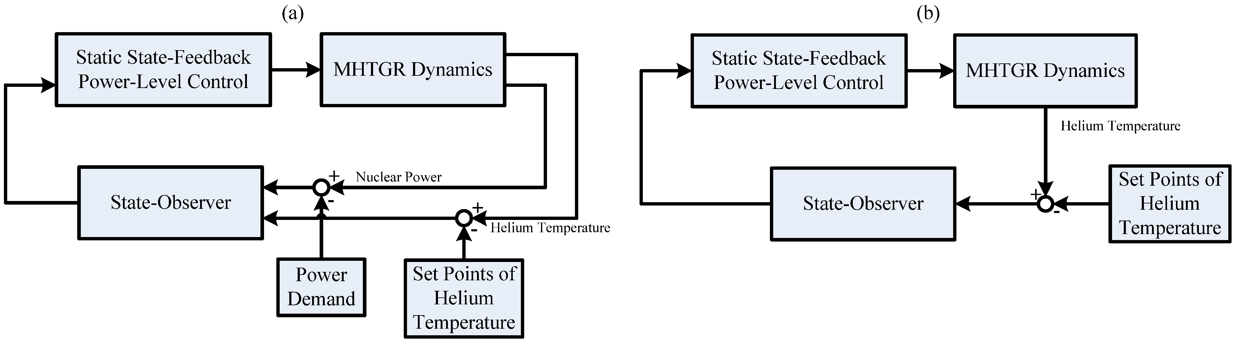
With this in mind, a novel nonlinear state observer providing globally convergent observation is proposed in this paper. It is proven that this observer is globally convergent if there is no disturbance, and has the L₂ disturbance attenuation performance in case of nonzero disturbance. Moreover, the separation principle of this observer is also proven, which means that it can recover the performance of a globally asymptotic stabilizer and that of an L₂ disturbance attenuator. A new nonlinear dynamic output feedback power-level control law which consists of this observer and the IDA-PLC given in [14] is then established. Numerical simulation results with discussion are finally given, which show both the feasibility and the satisfactory performance of this newly-built power-level control law. The structures of the feedback loops of the dynamic output feedback power-level control strategies presented in [14] and this paper are shown in Figure 3. Figure 3(a) shows the feedback loop in [14], and Figure 3(b) shows the feedback loop in this paper, which means that the control strategy given in this paper needs less measurement information than those in [13] and [14] need.

Figure 3. Structures of feedback loops.

Figure 3. Structures of feedback loops.

2. Problem Formulation

2.1. Nonlinear State-Space Model

To carry out the problem formulation, it is necessary to introduce the nonlinear state space model used for observer design and controller formulation. Here, the dynamic model of the MHTGR can be written as [13,14,17]:

$$\{\begin{array}{l}{\stackrel{\cdot }{n}}_{\text{r}}=\frac{{\rho }_{\text{r}}-\beta }{\Lambda }{n}_{\text{r}}+\frac{\beta }{\Lambda }{c}_{\text{r}}+\frac{n_{\text{r}}}{\Lambda }\left[{\alpha }_{\text{c}}\left(T_{\text{c}}-T_{\text{c},\text{m}}\right)+{\alpha }_{\text{r}}\left(T_{\text{r}}-T_{\text{r},\text{m}}\right)\right],\\ {\stackrel{\cdot }{c}}_{\text{r}}=\lambda \left(n_{\text{r}}-c_{\text{r}}\right),\\ {\stackrel{\cdot }{T}}_{\text{c}}=\frac{{\Omega }_{\text{cd}}}{{\mu }_{\text{c}}}\left(T_{\text{c}}-T_{\text{d}}\right)-\frac{{\Omega }_{\text{cr}}}{{\mu }_{\text{c}}}\left(T_{\text{c}}-T_{\text{r}}\right)+\frac{P_0}{{\mu }_{\text{c}}}{n}_r,\\ {\stackrel{\cdot }{T}}_{\text{d}}=\frac{2M_{\text{p}}}{{\mu }_{\text{d}}}\left(T_{\text{d}}-T_{\text{din}}\right)\text{+}\frac{{\Omega }_{\text{cd}}}{{\mu }_{\text{d}}}\left(T_{\text{c}}-T_{\text{d}}\right)，\\ {\stackrel{\cdot }{\rho }}_{\text{r}}\text{=}{G}_{\text{r}}{z}_{\text{r}},\end{array}$$

(1)

where n_r is the relative nuclear power, c_r is the relative concentration of delayed neutron precursor, β is the fraction of delayed fission neutrons, Λ (s⁻¹) is the effective prompt neutron life time, ρ_r is the reactivity given by the control rods, λ (s) is the effective radioactive decay constant of the delayed neutron precursor, α_c and α_r (1/°C) are respectively the reactivity coefficients of the fuel and reflector temperatures, P₀ (W) is the rated reactor thermal power, T_c (°C)is the average fuel temperature, T_d (°C) is the average temperature of the helium inside the pebble-bed, T_din (°C) is the temperature of the helium entering into the pebble-bed, T_c,m and T_d,m are initial equilibrium values of T_c and T_d respectively, T_r (°C) is the reflector temperature, Ω_cd and Ω_cr (W/°C) are respectively the heat transfer coefficient between the fuel and helium in the pebble-bed and that between the fuel and reflector inside the riser, M_p (W/°C) is the mass flowrate times the heat capacity of the helium inside the primary loop, μ_c and μ_d (Ws/°C) are respectively the total heat capacities of the fuel and the helium inside the reactor, G_r is the differential reactivity worth of the control rod, and z_r is the rod speed signal. To obtain the state-space model for observer design, the deviations of the actual values of n_r, c_r, T_c, T_d, T_din, T_r and ρ_r from their equilibrium values, i.e., n_r0, c_r0, T_c0, T_d0, T_din0, T_r0 and ρ_r0 are respectively defined as δn_r = n_r − n_r0, δc_r = c_r − c_r0, δT_c = T_c − T_c0, δT_d = T_d − T_d0, δT_din = T_din − T_din0, δT_r = T_r − T_r0 and δρ_r = ρ_r − ρ_r0.

Further, we define:

x = [δT_d δT_c δn_r δρ_r δc_r]^T

(2)

w = [δT_din δT_r]^T

(3)

and:

u = G_rz_r

(4)

Then, the nonlinear state space model utilized to design the state-observer can be written as:

$$\{\begin{array}{l}\stackrel{·}{\mathit{x}}=\mathit{f}(\mathit{x})+\mathit{g}u+\mathit{G}(\mathit{x})\mathit{w},\\ y=h(\mathit{x}),\end{array}$$

(5)

where:

$$\mathit{f}(\mathit{x})=\left[\begin{array}{c}-\frac{{\Omega }_{\text{cd}}\text{+}2M_{\text{p}}}{2}{x}_1+\frac{{\Omega }_{\text{cd}}}{{\mu }_{\text{d}}}{x}_2\\ \frac{{\Omega }_{\text{cd}}}{{\mu }_{\text{c}}}{x}_1-\frac{{\Omega }_{\text{cd}}+{\Omega }_{\text{cr}}}{{\mu }_{\text{c}}}{x}_2+\frac{P_{\text{0}}}{{\mu }_{\text{c}}}{x}_3\\ -\frac{\beta }{\Lambda }\left(x_3-x_5\right)+\frac{n_{\text{r}0}+x_3}{\Lambda }\left({\alpha }_{\text{c}}{x}_2+x_4\right)\\ \lambda \left(x_3-x_5\right)\end{array}\right]$$

(6)

g = [0 0 0 1 0]^T

(7)

$$\mathit{G}(\mathit{x})={\left[\begin{array}{ccccc}\frac{2M_{\text{p}}}{{\mu }_{\text{d}}}& 0& 0& 0& 0\\ 0& \frac{{\Omega }_{\text{cr}}}{{\mu }_{\text{c}}}& \frac{{\alpha }_{\text{r}}}{\Lambda }\left(n_{\text{r}0}+x_3\right)& 0& 0\end{array}\right]}^{\text{T}}$$

(8)

and:

h(x) = x₁

(9)

It is worth noting that the heat capacity of the reflector of the MHTGR is so large that δT_r varies very slowly, and δT_din reflects the influence of the other parts of the MHTGR to the reactor core dynamics. Therefore, it is quite reasonable to view w defined in Equation (3) as a disturbance.

2.2. Problem Formulation

Choose the state-observer corresponding to system (5) as:

$$\stackrel{\cdot }{\hat{\mathit{x}}}=\mathit{f}(\hat{\mathit{x}})+\mathit{g}u+\mathit{F}\left[y-h(\hat{\mathit{x}})\right]$$

(10)

where $\hat{x}\in {\text{R}}^5$ is the state-observation, vector-valued function f is determined by (6), g and h are given by (7) and (9) respectively, and here F is the observer gain to be designed.

From Equations (5) and (10), it is easy to obtain the dynamic equation of observation error defined by:

$$\mathit{e}\stackrel{△}{=}\mathit{x}-\hat{\mathit{x}}={\left[\begin{array}{ccccc}{e}_1& e_2& e_3& e_4& e_5\end{array}\right]}^{\text{T}}$$

(11)

i.e.:

$$\stackrel{\cdot }{\mathit{e}}={\mathit{f}}_{\text{e}}\left(\mathit{e}\right)-\mathit{F}{e}_1+\mathit{G}\left(\mathit{x}\right)\mathit{w}$$

(12)

where:

$${\mathit{f}}_e\left(\mathit{e}\right)=\mathit{f}\left(\mathit{x}\right)-\mathit{f}\left(\hat{\mathit{x}}\right)$$

(13)

Equation (13) can be easily satisfied since the vector-valued function f defined by (6) is clearly analytic.Furthermore, in order to form the theoretical problem to be solved, the concept of disturbance attenuation observer is firstly introduced as follows.

Definition 1 (L₂ Disturbance Attenuation Observer).

Consider the following nonlinear system:

$$\{\begin{array}{l}\stackrel{\cdot }{\mathit{\chi }}=\mathit{\omega }(\mathit{\chi })+\mathit{\zeta }(\mathit{\chi })\mathit{\upsilon }+\mathit{\Gamma }(\mathit{\chi })\mathit{d}\\ \mathit{\theta }=\mathit{\eta }(\mathit{\chi })\end{array}$$

(14)

where χ ∈ Rⁿ is the state vector, υ ∈ R^p is the input, θ ∈ R^m is the system output, d ∈ R^q is the disturbance, functions ω, ζ, η and Γ are all smooth, and ω(O) = O. Suppose the state observer of system (14) takes the form:

$$\stackrel{\cdot }{\hat{\mathit{x}}}=\mathit{\omega }(\hat{\mathit{\chi }})+\mathit{\zeta }(\hat{\mathit{\chi }})\mathit{\upsilon }+\mathit{\Lambda }\left[\mathit{\theta }-\mathit{\eta }(\hat{\mathit{\chi }})\right]$$

(15)

where $\hat{\chi }$ ∈ Rⁿ is the observer state, Λ is the observer gain. Define the evaluation signal of observer (15) as:

$$\mathit{\mu }\stackrel{\Delta }{=}\mathit{\mu }\left(\mathit{\tau }\right)$$

(16)

where τ is the observation error satisfying:

$$\tau =\chi -\hat{\chi }$$

(17)

State observer (15) is called an L₂ disturbance attenuation observer if there exists a semi-positive function Ω(τ), such that the following γ-dissipation inequality:

$$\stackrel{\cdot }{\Omega }\left(\mathit{\tau }\right)+\Phi \left(\mathit{\tau }\right)\le \frac{1}{2}\left({\gamma }^2{\Vert \mathit{d}\Vert }_2^2-{\Vert \mathit{\mu }\Vert }_2^2\right)$$

(18)

is satisfied, where Φ(τ) is a semi-positive function, ||·||₂ is the Euclidean norm, and γ is a positive scalar called the L₂ gain from disturbance d to evaluation signal μ. ☐

Finally, the theoretical problem to be solved in the following parts is formulated as follows:

Problem 1.

How to design the gain of observer (10) so that it has the L₂ disturbance attenuation performance if disturbance w ≠ O, and is globally convergent if w ≡ O? Moreover, under what conditions can this observer be coupled in the feedback loop and recover the performance of a state-feedback regulator?

3. Observer Design with Performance Analysis

3.1. Disturbance Attenuation and Convergence

This subsection focuses on solving the first part of Problem 1, i.e., finding a proper observer gain L such that (10) is an L₂ disturbance attenuation observer if disturbance w ≠ O, and is globally convergent if w ≡ O. The result is summarized as following Theorem 1, which is the first main result of this paper.

Theorem 1.

Consider state-observer (10) of MHTGR dynamics (5). Suppose that observer gain matrix F of observer (10) takes the form as:

F = [F₁ 0 F₂ 0 0]^T

(19)

where both F₁ and F₂ are positive scalars. Choose the evaluation signal corresponding to observer (10) as:

z = [e₁ e₃]^T

(20)

where e₁ and e₃ are defined in equation (11). Since δρ_r0 = 0, it is not loss of generality to assume that:

$${\hat{x}}_{4,0}=x_{4,0}=\mathsf{\delta }{\rho }_{\text{r}0}\text{=}0$$

(21)

where ${\hat{x}}_{4,0}$, x_4,0 and δ_ρr0 are the initial values of ${\hat{x}}_4$, x₄ and δ_ρr respectively. Then, state-observer (10) is an L₂ disturbance attenuation observer when w ≠ O if:

(a)

${\hat{x}}_{1,0}=x_{1,0}$, and

(b)

both positive scalars F₁ and F₂ are large enough.

Proof:

Substituting (19) into the observation error dynamics (12), and it is easy to see that:

$$\{\begin{array}{l}{\mu }_{\text{d}}{\stackrel{\cdot }{e}}_1=-{\Omega }_{\text{cd}}\left(e_1-e_2\right)-2M_{\text{p}}{e}_1-{\mu }_{\text{d}}{F}_1{e}_1+2M\mathsf{\delta }{T}_{\text{din}}\\ {\mu }_{\text{c}}{\stackrel{\cdot }{e}}_2={\Omega }_{\text{cd}}\left(e_1-e_2\right)-{\Omega }_{\text{cr}}{e}_2+P_0{e}_3+{\Omega }_{\text{cr}}\mathsf{\delta }{T}_{\text{r}}\\ \Lambda {\stackrel{\cdot }{e}}_3=-\beta \left(e_3-e_5\right)+\left(n_{\text{r}0}\text{+}{x}_3\right)\left({\alpha }_{\text{c}}{e}_2\text{+}{e}_4\right)+\left({\alpha }_{\text{c}}{\hat{x}}_2+{\hat{x}}_4\right)e_3-\Lambda F_2{e}_1+{\alpha }_{\text{r}}\left(n_{\text{r}0}\text{+}{x}_3\right)\mathsf{\delta }{T}_{\text{r}}\\ {\stackrel{\cdot }{e}}_4=0\\ {\stackrel{\cdot }{e}}_5=\lambda \left(e_3-e_5\right)\end{array}$$

(22)

From assumption (21) and the 4^th equation of (22), we have:

e₄ = 0

(23)

Substituting Equation (23) into (22), we can obtain that:

$$\{\begin{array}{l}{\mu }_{\text{d}}\stackrel{\cdot }{e_1}=-{\Omega }_{\text{cd}}\left(e_1-e_2\right)-2M_{\text{p}}{e}_1-{\mu }_{\text{d}}{F}_1{e}_1+2M_{\text{p}}\mathsf{\delta }{T}_{\text{din}}\\ {\mu }_{\text{c}}\stackrel{\cdot }{e_2}={\Omega }_{\text{cd}}\left(e_1-e_2\right)-{\Omega }_{\text{cr}}{e}_2+P_0{e}_3+{\Omega }_{\text{cr}}\mathsf{\delta }{T}_r\\ \Lambda {\stackrel{\cdot }{e}}_3=-\beta \left(e_3-e_5\right)+{\alpha }_{\text{c}}\left(n_{r0}+x_3\right)e_2+\left({\alpha }_{\text{c}}{\hat{x}}_2+{\hat{x}}_4\right)e_3-\Lambda F_2{e}_1\text{+}{\alpha }_{\text{r}}\left(n_{\text{r}0}+x_3\right)\mathsf{\delta }{T}_{\text{r}}\\ {\stackrel{\cdot }{e}}_5=\lambda \left(e_3-e_5\right)\end{array}$$

(24)

It is clear that the first two equations of (24) govern the observation error dynamics related to thermal-hydraulics of the MHTGR, and the other two equations is related to the neutron kinetics.

Choosing the Lyapunov function corresponding to the first two equations of (24) as:

$$V_{e1}\left(e_1,e_2\right)=\frac{1}{2}\left({\mu }_{\text{d}}{e}_1^2+{\mu }_{\text{c}}{e}_2^2\right)$$

(25)

and differentiating (25) along the trajectory given by the first two equations of (24):

$$\begin{array}{ll}{\stackrel{\cdot }{V}}_{e1}& ={\mu }_{\text{d}}{e}_1{e}_1+{\mu }_{\text{c}}{e}_2{e}_2\\ & =-{\Omega }_{\text{cd}}{\left(e_1-e_2\right)}^2-\left(2M_{\text{p}}+{\mu }_{\text{d}}{F}_1\right)e_1^2-{\Omega }_{\text{cr}}{e}_2^2+P_0{e}_2{e}_3+2M_{\text{p}}{e}_1\mathsf{\delta }{T}_{\text{din}}+{\Omega }_{\text{cr}}{e}_2\mathsf{\delta }{T}_{\text{r}}\end{array}$$

(26)

To formulate the Lyapunov function for the entire observation error dynamics, we need to analyze the property of term e₁e₃ in the following. Differentiate e₁e₃ along the trajectory determined by (24), and we can see that:

$$\begin{array}{l}\frac{\text{d}}{\text{d}t}\left(e_1{e}_3\right)={\stackrel{\cdot }{e}}_1{e}_3+e_1{\stackrel{\cdot }{e}}_3\\ =\left[-\frac{{\Omega }_{\text{cd}}}{{\mu }_{\text{d}}}\left(e_1-e_2\right)-\frac{2M_{\text{p}}}{{\mu }_{\text{d}}}{e}_1-F_1{e}_1+\frac{2M_{\text{p}}}{{\mu }_{\text{d}}}\mathsf{\delta }{T}_{\text{din}}\right]e_3+\\ e_1\left[-\frac{\beta }{\Lambda }\left(e_3-e_5\right)+\frac{{\alpha }_{\text{c}}}{\Lambda }{e}_2\left(n_{\text{r}0}\text{+}{x}_3\right)+\frac{{\alpha }_{\text{c}}\widehat{x_2}+\widehat{x_4}}{\Lambda }{e}_3-F_2{e}_1+\frac{{\alpha }_{\text{r}}}{\Lambda }\left(n_{\text{r}0}\text{+}{x}_3\right)\mathsf{\delta }{T}_{\text{r}}\right]\\ =-\left(\frac{{\Omega }_{\text{cd}}+2M_{\text{p}}}{{\mu }_{\text{d}}}+\frac{\beta }{\Lambda }+F_1-\frac{{\alpha }_{\text{c}}\widehat{x_2}+\widehat{x_4}}{\Lambda }\right)e_1{e}_3-F_2{e}_1^2+\frac{{\Omega }_{\text{cd}}}{{\mu }_{\text{d}}}{e}_2{e}_3\frac{2M_{\text{p}}}{{\mu }_{\text{d}}}{e}_3\mathsf{\delta }{T}_{\text{din}}+\\ \frac{1}{\Lambda }\left(n_{\text{r}0}+x_3\right)\left({\alpha }_{\text{c}}{e}_2+{\alpha }_{\text{r}}\mathsf{\delta }{T}_{\text{r}}\right)e_1\end{array}$$

(27)

From differential Equation (27), we have:

$$e_1{e}_3=c_0{e}^{-\kappa t}+\underset{0}{\overset{t}{\int }}{e}^{-\kappa \left(t-s\right)}\left[-F_2{e}_1^2+\frac{{\Omega }_{\text{cd}}}{{\mu }_{\text{d}}}{e}_2{e}_3+\frac{2M_{\text{p}}}{{\mu }_{\text{d}}}{e}_3\mathsf{\delta }{T}_{\text{din}}+\frac{1}{\Lambda }\left(n_{\text{r}0}+x_3\right)\left({\alpha }_{\text{c}}{e}_2+{\alpha }_{\text{r}}\mathsf{\delta }{T}_{\text{r}}\right)e_1\right]\text{d}s$$

(28)

where c₀ is the initial value of term e₁e₃, and:

$$\kappa \stackrel{\Delta }{\text{=}}\frac{{\Omega }_{\text{cd}}+2M_{\text{p}}}{{\mu }_{\text{d}}}+\frac{\beta }{\Lambda }+F_1-\frac{{\alpha }_{\text{c}}\widehat{x_2}+\widehat{x_4}}{\Lambda }$$

(29)

Suppose observer gains L₁ and L₂ are large enough so that:

$$\kappa \stackrel{\Delta }{\text{=}}\frac{{\Omega }_{\text{cd}}+2M_{\text{p}}}{{\mu }_{\text{d}}}+\frac{\beta }{\Lambda }+F_1-\frac{{\alpha }_{\text{c}}\widehat{x_2}+\widehat{x_4}}{\Lambda }>{\epsilon }_1$$

(30)

and:

$$F_2{e}_1^2-\frac{{\Omega }_{\text{cd}}}{{\mu }_{\text{d}}}{e}_2{e}_3+\frac{2M_{\text{p}}}{{\mu }_{\text{d}}}{e}_3\mathsf{\delta }{T}_{\text{din}}+\frac{1}{\Lambda }\left(n_{\text{r}0}+x_3\right)\left({\alpha }_{\text{c}}{e}_2+{\alpha }_{\text{r}}\mathsf{\delta }{T}_{\text{r}}\right)e_1>{\epsilon }_2{e}_1^2$$

(31)

where both ε₁ and ε₂ are positive scalars.

Substituting inequalities (30) and (31) into (28):

$$\begin{array}{l}{e}_1{e}_3<c_0{e}^{-{\epsilon }_{1}t}-{\epsilon }_2\underset{0}{\overset{t}{\int }}{e}^{-{\epsilon }_1(t-s)}{e}_1^2(s)\text{d}s=c_0{e}^{-{\epsilon }_{1}t}-{\epsilon }_2{e}_1^2(\sigma )\underset{0}{\overset{t}{\int }}{e}^{-{\epsilon }_1(t-s)}\text{d}s\\ =c_0{e}^{-{\epsilon }_{1}t}-\frac{{\epsilon }_2}{{\epsilon }_1}{e}_1^2(\sigma )(1-e^{-{\epsilon }_{1}t})=\left[c_0+\frac{{\epsilon }_2}{{\epsilon }_1}{e}_1^2(\sigma )\right]e^{-{\epsilon }_{1}t}-\frac{{\epsilon }_2}{{\epsilon }_1}{e}_1^2(\sigma )\end{array}$$

(32)

where σ ∈ (0,t).

From inequality (32), if:

$$c_0+\frac{{\epsilon }_2}{{\epsilon }_1}{e}_1^2(\sigma )=0$$

it is clear that e₁e₃ < 0. Further, if:

$$c_0+\frac{{\epsilon }_2}{{\epsilon }_1}{e}_1^2(\sigma )\ne 0$$

then, from inequality (32), it is clear that e₁e₃ < 0 when:

$$t>\frac{1}{{\epsilon }_1}\ln \left[\frac{{\epsilon }_1{c}_0}{{\epsilon }_2{e}_1^2(\sigma )}+1\right]$$

(33)

Since the inlet and outlet helium temperatures of the MHTGR can be measured, it is feasible to set:

$${\hat{x}}_{1,0}=x_{1,0}$$

i.e.:

c₀ = e₁₀e₃₀ = 0

(34)

where e₁₀ and e₃₀ are the initial values of e₁ and e₃ respectively. Based upon (33) and (34), it is so clear that e₁e₃ < 0 for any t > 0 if inequality (31) is satisfied. Since e₁e₃ can be negative definite for any t > 0, it is then possible for us to construct the whole Lyapunov function and guarantee the L₂ disturbance attenuation performance for observer (10). The detail derivation is given as follows.

If we choose the Lyapunov function for the entire observation error dynamics as:

$$V_e=\frac{V_{\text{e1}}}{P_{\text{0}}}-\frac{{\mu }_{\text{d}}}{{\Omega }_{\text{cd}}}{e}_{\text{1}}{e}_{\text{3}}$$

(35)

and then differentiate it along the trajectory given by the observation error dynamics:

$$\begin{array}{l}{\stackrel{\cdot }{V}}_e=\frac{{\stackrel{\cdot }{V}}_{e1}}{P_0}-\frac{{\mu }_{\text{d}}}{{\Omega }_{\text{cd}}}\frac{\text{d}}{\text{d}t}(e_1{e}_3)\\ =-\frac{{\Omega }_{\text{cd}}}{P_0}{(e_1-e_2)}^2-\frac{2M_{\text{P}}+{\mu }_{\text{d}}{F}_1}{P_0}{e}_1^2-\frac{{\Omega }_{\text{cr}}}{P_0}{e}_2^2+e_2{e}_3+\frac{2M_{\text{P}}}{P_0}{e}_1\mathsf{\delta }{T}_{\text{din}}+\frac{{\Omega }_{\text{cr}}}{P_0}{e}_2\mathsf{\delta }{T}_{\text{r}}+\\ \frac{{\mu }_{\text{d}}}{{\Omega }_{\text{cd}}}\left(\frac{{\Omega }_{\text{cd}}+2M_{\text{P}}}{{\mu }_{\text{d}}}+\frac{\beta }{\Lambda }+F_1-\frac{{\alpha }_{\text{c}}{\hat{x}}_2+{\hat{x}}_4}{\Lambda }\right)e_1{e}_3+\frac{{\mu }_{\text{d}}}{{\Omega }_{\text{cd}}}{F}_2{e}_1^2-e_2{e}_3-\frac{2M_{\text{P}}}{{\Omega }_{\text{cd}}}{e}_3\mathsf{\delta }{T}_{\text{din}}-\frac{{\alpha }_{\text{c}}{\mu }_{\text{d}}}{\Lambda {\Omega }_{\text{cd}}}\left(n_{\text{r}0}+x_3\right)\left(e_2+\frac{{\alpha }_{\text{r}}}{{\alpha }_{\text{c}}}\mathsf{\delta }{T}_{\text{r}}\right)\\ \le -\frac{{\Omega }_{\text{cd}}}{P_0}{(e_1-e_2)}^2-\left[\frac{{\mu }_{\text{d}}{F}_1}{P_0}+\frac{2M_{\text{P}}}{P_0}\left(1-\frac{2M_{\text{P}}}{{\gamma }^2{P}_0}\right)-\frac{{\mu }_{\text{d}}}{{\Omega }_{\text{cd}}}{F}_2-\frac{1}{2}\right]e_1^2-\frac{{\Omega }_{\text{cr}}}{P_0}\left(1-\frac{{\Omega }_{\text{cr}}}{2{\gamma }^2{P}_0}\right)e_2^2+\left(\frac{1}{2}+\frac{4M_{\text{P}}^2}{{\gamma }^2{\Omega }_{\text{cd}}^2}\right)e_3^2+\\ \frac{{\mu }_{\text{d}}}{{\Omega }_{\text{cd}}}\left(\frac{{\Omega }_{\text{cd}}+2M_{\text{P}}}{{\mu }_{\text{d}}}+\frac{\beta }{\Lambda }+F_1-\frac{{\alpha }_{\text{c}}{\hat{x}}_2+{\hat{x}}_4}{\Lambda }\right)e_1{e}_3-\frac{{\alpha }_{\text{c}}{\mu }_{\text{d}}}{\Lambda {\Omega }_{\text{cd}}}\left(n_{\text{r}0}\text{+}{x}_3\right)e_1\left(e_2+\frac{{\alpha }_{\text{r}}}{{\alpha }_{\text{c}}}\mathsf{\delta }{T}_{\text{r}}\right)\text{+}\frac{1}{2}\left({\gamma }^2{\Vert \mathit{w}\Vert }_2^2-{\Vert \mathit{z}\Vert }_2^2\right).\end{array}$$

(36)

For the MHTGR, we have the following physical relationship, i.e.:

Ω_cr << M_p << P₀

(37)

It is natural to assume that:

$$\gamma >\max \{\sqrt{\frac{2M_{\text{P}}}{P_0}},\sqrt{\frac{{\Omega }_{\text{cr}}}{2P_0}}\}$$

(38)

and then from the negative definite property of e₁e₃, there must be a large enough F₁ satisfying:

$$\left(\frac{{\Omega }_{\text{cd}}+2M_{\text{P}}}{{\mu }_{\text{d}}}+\frac{\beta }{\Lambda }+F_1-\frac{{\alpha }_{\text{c}}{\hat{x}}_2+{\hat{x}}_4}{\Lambda }\right)e_1{e}_3+\left(F_2+\frac{{\Omega }_{\text{cd}}}{2{\mu }_{\text{d}}}\right)e_1^2+\left(\frac{{\Omega }_{\text{cd}}}{2{\mu }_{\text{d}}}+\frac{4M_{\text{P}}^2}{{\gamma }^2{\mu }_{\text{d}}{\Omega }_{\text{cd}}}\right)e_3^2-\frac{n_{\text{r}0}+x_3}{\Lambda }{e}_1\left({\alpha }_{\text{c}}{e}_2+{\alpha }_{\text{r}}\mathsf{\delta }{T}_{\text{r}}\right)<{\epsilon }_3{e}_1{e}_3$$

(39)

where ε₃ is a positive scalar.

Based upon inequalities (36), (38) and (39), we have:

$${\stackrel{\cdot }{V}}_e<{\gamma }^2{\Vert \mathit{w}\Vert }_2^2-{\Vert \mathit{z}\Vert }_2^2-\frac{{\Omega }_{\text{cd}}}{P_0}{(e_1-e_2)}^2-\frac{{\mu }_{\text{d}}{F}_1}{P_0}{e}_1^2+\frac{{\mu }_{\text{d}}}{{\Omega }_{\text{cd}}}{\epsilon }_3{e}_1{e}_3<{\gamma }^2{\Vert \mathit{w}\Vert }_2^2-{\Vert \mathit{z}\Vert }_2^2$$

(40)

From Definition 1, we can see that observer (10) has the performance of F₂ disturbance attenuation, which completes the proof of this theorem. ☐

Remark 1:

Here, it is clear that if e₁ ≠ 0 (t > 0), then there must exist a gain F₂ such that inequality (31) is well satisfied. Otherwise, substitute e₁ = 0 (t > 0) to the first two equations of (24):

$$\mathsf{\delta }{\stackrel{\cdot }{T}}_{\text{din}}=-\frac{{\Omega }_{\text{cd}}\text{+}{\Omega }_{\text{cr}}}{{\mu }_{\text{c}}}\mathsf{\delta }{T}_{\text{din}}+\frac{2M_{\text{p}}{P}_0}{{\mu }_{\text{c}}{\Omega }_{\text{cd}}}{e}_3+\frac{2M_{\text{p}}{\Omega }_{\text{cr}}}{{\mu }_{\text{c}}{\Omega }_{\text{cd}}}\mathsf{\delta }{T}_{\text{r}}$$

(41)

Since the dynamics of δT_din are related directly with the variations of the outlet helium temperature and the mean steam temperature in the secondary loop of the steam generator, which means that it has no direct relationship with e₃ and δT_r, Equation (41) can be only satisfied if δT_din = δT_r = e₃ = 0, which contradicts with w ≠ O. Thus, it is no loss of generality to suppose that there exists a large enough F₂ such that inequality (31) is satisfied. ☐

Remark 2:

Observer gains F₁ and F₂ are large enough means that inequalities (30), (31) and (39) are all satisfied. The function of F₂ is to guarantee that e₁e₃ < 0 for any t > 0, and the function of gain L₁ is to guarantee the disturbance attenuation performance of observer (10). Moreover, from inequality (39), it is clear that smaller L₂ gain γ needs larger observer gain F₁. ☐

From Theorem 1, we know that state-observer (10) has the L₂ disturbance attenuation performance when w ≠ O. The following Theorem 2, which is the second main result of this paper, gives the sufficient condition for state-observer (10) to be globally convergent.

Theorem 2.

Consider state-observer (10) of MHTGR dynamics (5) with gain matrix F taking the form as (19). Suppose (21) is well satisfied, and assume that w = O. Then observer (10) is globally convergent if conditions a) and b) in Theorem 1 are both satisfied.

Proof:

Substitute w = O to (24), and the observation error dynamics can then be written as:

$$\{\begin{array}{l}{\mu }_{\text{d}}{\stackrel{\cdot }{e}}_1=-{\Omega }_{\text{cd}}\left(e_1-e_2\right)-2M_{\text{P}}{e}_1-{\mu }_{\text{d}}{F}_1{e}_1\\ {\mu }_{\text{c}}{\stackrel{\cdot }{e}}_2={\Omega }_{\text{cd}}\left(e_1-e_2\right)-{\Omega }_{\text{cr}}{e}_2+P_0{e}_3\\ \Lambda {\stackrel{\cdot }{e}}_3=-\beta \left(e_3-e_5\right)+{\alpha }_{\text{c}}\left(n_{\text{r}0}\text{+}{x}_3\right)e_2+\left({\alpha }_{\text{c}}{\hat{x}}_2+{\hat{x}}_4\right)e_3-\Lambda F_2{e}_1\\ {\stackrel{\cdot }{e}}_5=\lambda \left(e_3-e_5\right)\end{array}$$

(42)

Choose the Lyapunov function of the first two equations of (42) as (25), and differentiate it along the trajectory given by (42):

$${\stackrel{\cdot }{V}}_{\text{e}1}\text{=}{\mu }_{\text{d}}{e}_1{e}_1+{\mu }_{\text{c}}{e}_2{e}_2=-{\Omega }_{\text{cd}}{\left(e_1-e_2\right)}^2-\left(2M_{\text{p}}+{\mu }_{\text{d}}{F}_1\right)e_1^2-{\Omega }_{\text{cr}}{e}_2^2{P}_0{e}_2{e}_3$$

(43)

Moreover, differentiating e₁e₃, i.e.:

$$\frac{\text{d}}{\text{d}t}\left(e_1{e}_3\right)=-\left(\frac{{\Omega }_{\text{cd}}+2M_{\text{p}}}{{\mu }_{\text{d}}}+\frac{\beta }{\Lambda }+F_1-\frac{{\alpha }_{\text{c}}{\hat{x}}_2+{\hat{x}}_4}{\Lambda }\right)e_1{e}_3-F_2{e}_1^2+\frac{{\Omega }_{\text{cd}}}{{\mu }_{\text{d}}}{e}_2{e}_3+\frac{{\alpha }_{\text{c}}}{\Lambda }\left(n_{\text{r}0}\text{+}{x}_3\right)e_1{e}_2$$

(44)

From (44), it is clear that:

$$e_1{e}_3=c_0{e}^{-\kappa t}+\underset{0}{\overset{t}{\int }}{e}^{-\kappa \left(t-s\right)}\left[-F_2{e}_1^2+\frac{{\Omega }_{\text{cd}}}{{\mu }_{\text{d}}}{e}_2{e}_3+\frac{{\alpha }_{\text{c}}}{\Lambda }\left(n_{\text{r}0}\text{+}{x}_3\right)e_1{e}_2\right]\text{d}s$$

(45)

where c₀ is the initial value of term e₁e₃, and κ is also defined by (29).

In the following, we should discuss in the cases of e₁ ≠ 0 and e₁ = 0 for any t > 0.

If e₁ ≠ 0 (t > 0), then there exists large enough observer gains F₁ and F₂ are so that inequalities (30) and:

$$F_2{e}_1^2-\frac{{\Omega }_{\text{cd}}}{{\mu }_{\text{d}}}{e}_2{e}_3+\frac{{\alpha }_{\text{c}}}{\Lambda }\left(n_{\text{r}0}\text{+}{x}_3\right)e_2>{\epsilon }_4{e}_1^2$$

(46)

where ε₄ is a positive scalar, are well satisfied, then from (45) and assumption (21), we have:

$$e_1{e}_3<-\frac{{\epsilon }_2}{{\epsilon }_1}{e}_1^2(\sigma )(1-e^{-{\epsilon }_{1}t})$$

(47)

where σ ∈ (0,t).

Similarly to the proof of Theorem 1, we set the Lyapunov function of the entire error system (42) as (35), and then differentiate it along the trajectory given by (42):

$$\begin{array}{l}{\stackrel{\cdot }{V}}_{\text{e}}\le -\frac{{\Omega }_{\text{cd}}}{P_0}{(e_1-e_2)}^2-\left[\frac{2M_{\text{p}}+{\mu }_{\text{d}}{F}_1}{P_0}-\frac{{\mu }_{\text{d}}}{{\Omega }_{\text{cd}}}{F}_2\right]e_1^2-\frac{{\Omega }_{\text{cr}}}{P_0}{e}_2^2-\frac{{\alpha }_{\text{c}}{\mu }_{\text{d}}}{\Lambda {\Omega }_{\text{cd}}}\left(n_{\text{r}0}\text{+}{x}_3\right)e_1{e}_2\text{+}\\ \frac{{\mu }_{\text{d}}}{{\Omega }_{\text{cd}}}\left(\frac{{\Omega }_{\text{cd}}\text{+}2M_{\text{p}}}{{\mu }_{\text{d}}}\text{+}\frac{\beta }{\Lambda }+F_1-\frac{{\alpha }_{\text{c}}{\hat{x}}_2+{\hat{x}}_4}{\Lambda }\right)e_1{e}_3\end{array}$$

(48)

Also, from the negative definition of e₁e₃, there must exist a large enough F₁ satisfying:

$$\left(\frac{{\Omega }_{\text{cd}}\text{+}2M_{\text{p}}}{{\mu }_{\text{d}}}\text{+}\frac{\beta }{\Lambda }+F_1-\frac{{\alpha }_{\text{c}}{\hat{x}}_2+{\hat{x}}_4}{\Lambda }\right)e_1{e}_3+F_2{e}_1^2+\frac{{\alpha }_{\text{c}}}{\Lambda }\left(n_{\text{r}0}\text{+}{x}_3\right)e_1{e}_2<{\epsilon }_5{e}_1{e}_3$$

(49)

where ε₅ is a positive scalar. Substitute (49) to (48), we have:

$${\stackrel{\cdot }{V}}_{\text{e}}<-\frac{{\Omega }_{\text{cd}}}{P_0}{(e_1-e_2)}^2-\frac{2M_{\text{p}}+{\mu }_{\text{d}}{F}_1}{P_0}{e}_1^2-\frac{{\Omega }_{\text{cr}}}{P_0}{e}_2^2\text{+}\frac{{\mu }_{\text{d}}}{{\Omega }_{\text{cd}}}{\epsilon }_5{e}_1{e}_3$$

(50)

From inequality (50), Equations (23) and (42), observation error e must be in the set defined by:

$$\Pi \stackrel{\Delta }{=}\left\{e| {\stackrel{\cdot }{e}}_5=-\lambda e_5, e_1=0, i=1,2,3,4\right\}$$

(51)

in which any e must converge to origin. From the Lassalle’s invariance principle, observer (10) is globally convergent in the case of e₁ ≠ 0 (t > 0).

Furthermore, if e₁ = 0 for any t > 0, then from (42):

$$\{\begin{array}{l}0=e_2\\ {\mu }_{\text{c}}{\stackrel{\cdot }{e}}_2=-\left({\Omega }_{\text{cd}}+{\Omega }_{\text{cr}}\right)e_2+P_0{e}_3\\ \Lambda {\stackrel{\cdot }{e}}_3=-\beta (e_3-e_5)+{\alpha }_{\text{c}}(n_{\text{r}0}\text{+}{x}_3)e_2+({\alpha }_{\text{c}}{\hat{x}}_2+{\hat{x}}_4)e_3\\ {\stackrel{\cdot }{e}}_5=\lambda (e_3-e_5)\end{array}$$

(52)

Then substituting the 1^st equation of (52) into the other three equations, we can easily see that e₁ = 0 means that the observation error e must in the set defined by (51). Also from the Lassalle’s invariance principle, observer (10) is globally convergent in the case of e₁ = 0 (t > 0).

This completes the proof of Theorem 2. ☐

Remark 3:

In Theorem 2, observer gains F₁ and F₂ are large enough means that inequalities (30), (46) and (49) are all well satisfied. ☐

Theorems 1 and 2 give us the solution to the first part of Problem 1 raised in Section 2, i.e., the method of adjusting the gain matrix F of observer (10) so that it is globally convergent in the case of e₁ = 0 (t > 0), and is the L₂ disturbance attenuation observer in the case of e₁ ≠ 0 (t > 0). In the following, we shall focus on whether observer (10) can recover the performance a well-designed power-level regulator of the MHTGR.

3.2. Performance Recovery

Here, observer (10) can recover the performance of a well-designed state-feedback power-level control if the dynamic output feedback power-level control strategy composed of this static state-feedback power-level regulator and observer (10) still keeps the key characteristics of this static state-feedback regulator such as the L₂ disturbance attenuation performance and asymptotic stability. Before giving the theoretical result about performance recovery, the definition of L₂ disturbance attenuator is given as follows:

Definition 2.

Consider nonlinear system (14) with evaluation signal defined as:

ξ = ξ(χ)

(53)

Control input u is said to be an L₂ disturbance attenuator if there is a semi-positive smooth function Σ(x) such that following ϑ-dissipation inequality:

$$\stackrel{\cdot }{\Sigma }(\mathit{\chi })+Q(\mathit{\chi })\le \frac{1}{2}\left({\vartheta }^2{\Vert \mathit{w}\Vert }_2^2-{\Vert \mathit{\xi }\Vert }_2^2\right)$$

(54)

is satisfied, where Q(x) is a semi-positive function, and $\vartheta$ is a positive scalar called the L₂ gain from disturbance w to evaluation signal ξ. □

The following theorem, i.e., the 3^rd main result of this paper tells us under what conditions can observer (10) recover the performance of an L₂ disturbance attenuator.

Theorem 3.

Consider MHTGR dynamics (5) with state-observer (10), and assume that the MHTGR is in the normal power operation, i.e.:

a < n_r = n_r0 + x₁ < b

(55)

where both a and b are given positive scalars. Suppose that static state feedback power-level control of the MHTGR taking the form:

u = Θ(x)

(56)

is an L₂ disturbance attenuator if disturbance w ≠ O, i.e., there exists a semi-positive differentiable function W₁ and an evaluation signal υ = υ(x) such that:

$${\stackrel{\cdot }{W}}_1(\mathit{x})+S(\mathit{x})\le \frac{1}{2}\left({\varsigma }^2{\Vert \mathit{w}\Vert }_2^2-{\Vert \mathit{\upsilon }\Vert }_2^2\right)$$

(57)

where S is a semi-positive function, and ς is a positive scalar denoting the L₂ gain from w to υ. Here, we assume that there exists a positive scalar M₁ such that:

$$\left|\frac{\partial W_1}{\partial x_1}\right|<M_1$$

(58)

Therefore dynamic output feedback power-level control:

$$\{\begin{array}{l}u=\Theta (\hat{\mathit{x}}),\\ \hat{\mathit{x}}=\mathit{f}(\hat{\mathit{x}})+\mathit{g}u+\mathit{F}[y-h(\hat{\mathit{x}})],\end{array}$$

(59)

where observer gain matrix F satisfies (19), is an L₂ disturbance attenuator in case of w ≠ O, if conditions (a) and (b) in Theorem 1 are both satisfied and:

(c)

function Θ satisfies:

$$\left|\Theta ({\mathit{x}}_1)-\Theta ({\mathit{x}}_2)\right|\le L{\Vert {\mathit{x}}_1-{\mathit{x}}_2\Vert }_2$$

(60)

where L is a positive scalar and x₁, x₂ Rⁿ satisfying (55) are two state-vectors of the MHTGR dynamics.

Proof:

First, we shall prove that dynamic output feedback power-level control law (59) can recover the L₂ disturbance attenuation performance of static state-feedback controller (56) if conditions (a), (b) and (c) of this theorem are all satisfied. Since condition (a) is satisfied and observer gain F₂ is high enough, it is quite clear that from the proof of Theorem 1 that e₁e₃ is definitely negative. The Lyapunov function for the entire system composed of MHTGR dynamics (5) and power-level control (59) can be chosen as:

V₁ = V_e + W₁

(61)

where V_e is determined by (35).

Differentiate V₁ along the trajectory given by (5) and (59), we have:

$$\begin{array}{l}{\stackrel{\cdot }{V}}_1={\stackrel{\cdot }{W}}_1{|}_{u=u(\hat{x})}+{\stackrel{\cdot }{V}}_e\\ ={\stackrel{\cdot }{W}}_1{|}_{u=u(x)}+{\stackrel{\cdot }{V}}_e+\frac{\partial W_1}{\partial \mathit{x}}\mathit{g}[u(\hat{\mathit{x}})-u(\mathit{x})]\\ \le -S(\mathit{x})-\frac{{\Omega }_{\text{cd}}}{P_0}{(e_1-e_2)}^2-\left[\frac{{\mu }_{\text{d}}{F}_1}{P_0}+\frac{2M_{\text{p}}}{P_0}\left(1-\frac{2M_{\text{p}}}{{\gamma }^2{P}_0}\right)-\frac{{\mu }_{\text{d}}}{{\Omega }_{\text{cd}}}{F}_2-\frac{1}{2}\right]e_1^2-\frac{{\Omega }_{\text{cr}}}{P_0}\left(1-\frac{{\Omega }_{\text{cr}}}{2{\gamma }^2{P}_0}\right)e_2^2+\\ \left(\frac{1}{2}+\frac{4M_{\text{p}}^2}{{\gamma }^2{\Omega }_{\text{cd}}^2}\right)e_3^2+\frac{{\mu }_{\text{d}}}{{\Omega }_{\text{cd}}}\left(\frac{{\Omega }_{\text{cd}}+2M_{\text{p}}}{{\mu }_{\text{d}}}+\frac{\beta }{\Lambda }+F_1-\frac{{\alpha }_{\text{c}}{\hat{x}}_2\text{+}{\hat{x}}_4}{\Lambda }\right)e_1{e}_3-\frac{{\alpha }_{\text{c}}{\mu }_{\text{d}}}{\Lambda {\Omega }_{\text{cd}}}\left(n_{\text{r}0}\text{+}{x}_3\right)e_1\left(e_2+\frac{{\alpha }_{\text{r}}}{{\alpha }_{\text{c}}}\mathsf{\delta }{T}_{\text{r}}\right)\text{+}\\ \frac{1}{2}\left({\gamma }^2{\Vert \mathit{w}\Vert }_2^2-{\Vert \mathit{z}\Vert }_2^2\right)+\frac{1}{2}\left({\varsigma }^2{\Vert \mathit{w}\Vert }_2^2-{\Vert \mathit{\upsilon }\Vert }_2^2\right)+\frac{\partial W_1}{\partial x_1}\left|\Theta (\mathit{x})-\Theta (\hat{\mathit{x}})\right|\end{array}$$

(62)

Further, from (60) and (58), we have:

$${\stackrel{\cdot }{V}}_1\le {\Vert \mathit{e}\Vert }_{\mathit{U}}^2+\frac{{\mu }_{\text{d}}}{{\Omega }_{\text{cd}}}\left(\frac{{\Omega }_{\text{cd}}+2M_{\text{p}}}{{\mu }_{\text{d}}}+\frac{\beta }{\Lambda }+F_1-\frac{{\alpha }_{\text{c}}{\hat{x}}_2\text{+}{\hat{x}}_4}{\Lambda }\right)e_1{e}_3-\frac{{\alpha }_{\text{c}}{\mu }_{\text{d}}}{\Lambda {\Omega }_{\text{cd}}}\left(n_{\text{r}0}\text{+}{x}_3\right)e_1\left(e_2+\frac{{\alpha }_{\text{r}}}{{\alpha }_{\text{c}}}\mathsf{\delta }{T}_{\text{r}}\right)\text{+}\frac{1}{2}\left({\varpi }^2{\Vert \mathit{w}\Vert }_2^2-{\Vert \mathit{\psi }\Vert }_2^2\right)$$

(63)

where:

$$\mathit{U}=\text{diag}\left(\left[M_{1}L+\frac{{\mu }_{\text{d}}}{{\Omega }_{\text{cd}}}{F}_2+\frac{1}{2} M_{1}L M_{1}L+\frac{4M_{\text{p}}^2}{{\gamma }^2{\Omega }_{\text{cd}}^2}+\frac{1}{2} 0 M_{1}L\right]\right)$$

(64)

$$\varpi =\sqrt{{\gamma }^2+{\varsigma }^2}$$

(65)

$$\mathit{\Psi }={\left[\begin{array}{cc}{\text{z}}^{\text{T}}& {\upsilon }^{\text{T}}\end{array}\right]}^{\text{T}}$$

(66)

Based upon (55), ||e||_U is definitely bounded and there must exist a large enough gain F₁ such that:

$$\left(\frac{{\Omega }_{\text{cd}}+2M_{\text{p}}}{{\mu }_{\text{d}}}+\frac{\beta }{\Lambda }+F_1-\frac{{\alpha }_{\text{c}}{\hat{x}}_2\text{+}{\hat{x}}_4}{\Lambda }\right)e_1{e}_3\text{+}{\Vert e\Vert }_U^2-\frac{{\alpha }_{\text{c}}{\mu }_{\text{d}}}{\Lambda {\Omega }_{\text{cd}}}\left(n_{\text{r}0}\text{+}{x}_3\right)e_1\left(e_2+\frac{{\alpha }_{\text{r}}}{{\alpha }_{\text{c}}}\mathsf{\delta }{T}_{\text{r}}\right)<{\epsilon }_6{e}_1{e}_3$$

(67)

where ε₆ is a positive scalar, then:

$${\stackrel{\cdot }{V}}_1-{\epsilon }_6{e}_1{e}_3\le \frac{1}{2}\left({\varpi }^2{\Vert \mathit{w}\Vert }_2^2-{\Vert \mathit{\psi }\Vert }_2^2\right)$$

(68)

Because of the negative definition of e₁e₃ and from the Definition 2, dynamic output feedback control strategy (59) is clearly an L₂ disturbance attenuator. This completes the proof of Theorem 3. ☐

In the following, we shall explore whether observer (10) can recover the performance of a global asymptotic stabilizer. Before giving the result, the inverse Lyapunov lemma is introduced as follows:

Lemma 1 

[18]. Consider an autonomous nonlinear system:

$$\stackrel{\cdot }{\mathit{\chi }}=\mathit{\omega }\left(\mathit{\chi }\right)$$

(69)

where χ ∈ Rⁿ is the state vector, ω: D ⊂ Rⁿ → Rⁿ is local Lipchitz, and ω(O) = O. Here, suppose that χ = O is a asymptotic stable steady point, and R_A ⊂ D is the attracting domain of χ = O. Therefore, for all χ ∈ R_A, there is smooth positive definite function ϒ(χ) and a continuous positive definite function W(χ) such that:

∈ ϒ (χ) → ∞, χ → ∂R_A

(70)

$$\frac{\partial \omega }{\partial \chi }\Upsilon (\chi )\le -W(\chi ), \forall \chi \in \partial R_{\text{A}}$$

(71)

and for any c > 0, {ϒ(χ) ≤ c} is a compact subset of R_A. If steady point χ = O is globally asymptotically stable, i.e., D = R_A = Rⁿ, then conditions (70) and (71) respectively change to:

ϒ(χ) → ∞, ||χ||₂ → ∞

(72)

$$\frac{\partial \Upsilon }{\partial \chi }\omega (\chi )\le -W(\chi ), \forall \chi \in {\text{R}}^n$$

(73)

Based upon Lemma 1, the following theorem, which is the 4^th main result of this paper, gives us the sufficient condition for observer (10) to recover the performance of a globally asymptotic stabilizer.

Theorem 4.

Consider MHTGR dynamics (5) with state-observer (10), and assume that the MHTGR is in normal power operation, i.e., (55) is satisfied. Suppose that static state feedback power-level control of the MHTGR (56) is a globally asymptotic stabilizer if disturbance w = O, i.e., there is a smooth positive definite function W₂(x) and a continuous positive definite function E(x) such that:

W₂(x) → ∞, ||x||₂ → ∞

(74)

$$\frac{\partial W_2}{\partial \mathit{x}}(\mathit{f}+\mathit{g}u)\le -E(\chi ), \forall \mathit{x}\in {\text{R}}^n$$

(75)

Moreover, we assume that there exists a positive scalar M₂ such that:

$$\left|\frac{\partial W_2}{\partial x_1}\right|<M_2$$

(76)

Therefore, dynamic output feedback power-level controller (59) is still a globally asymptotic stabilizer in case of w ≡ O, if conditions (a) and (b) in Theorem 1 and (c) in Theorem 2 are all satisfied.

Proof:

Similarly to the proof of Theorem 3, the whole Lyapunov function can be chosen as:

V₂ = V_e + W₂

(77)

where V_e is determined by (35) whose negative definition is provided by large enough observer gain F₂.

Differentiate V₂ along the trajectory given by (5) and (59):

$$\begin{array}{l}{\stackrel{\cdot }{V}}_1={\stackrel{\cdot }{W}}_2{|}_{u=\Theta (\hat{x})}+{\stackrel{\cdot }{V}}_e\\ ={\stackrel{\cdot }{W}}_2{|}_{u=\Theta (x)}+{\stackrel{\cdot }{V}}_e+\frac{\partial W_2}{\partial x}\mathit{g}[u(\hat{\mathit{x}})-u(\mathit{x})]\\ \le -E(x)-\frac{{\Omega }_{\text{cd}}}{P_0}{(e_1-e_2)}^2-\left[\frac{2M_{\text{p}}\text{+}{\mu }_{\text{d}}{F}_1}{P_0}-\frac{{\mu }_{\text{d}}}{{\Omega }_{\text{cd}}}{F}_2\right]e_1^2-\frac{{\Omega }_{\text{cr}}}{P_0}{e}_2^2-\frac{{\alpha }_{\text{c}}{\mu }_{\text{d}}}{\Lambda {\Omega }_{\text{cd}}}\left(n_{\text{r}0}\text{+}{x}_3\right)e_1{e}_2+\\ \frac{{\mu }_{\text{d}}}{{\Omega }_{\text{cd}}}\left(\frac{{\Omega }_{\text{cd}}+2M_{\text{p}}}{{\mu }_{\text{d}}}+\frac{\beta }{\Lambda }+F_1-\frac{{\alpha }_{\text{c}}{\hat{x}}_2\text{+}{\hat{x}}_4}{\Lambda }\right)e_1{e}_3+\frac{\partial W_2}{\partial x_1}\left|\Theta (\mathit{x})-\Theta (\hat{\mathit{x}})\right|\end{array}$$

(78)

Substituting (60) and (76) into (78), we have:

$$\begin{array}{l}{\stackrel{\cdot }{V}}_1\le -E(x)-\frac{{\Omega }_{\text{cd}}}{P_0}{(e_1-e_2)}^2-\frac{2M_{\text{p}}\text{+}{\mu }_{\text{d}}{F}_1}{P_0}{e}_1^2-\frac{{\Omega }_{\text{cr}}}{P_0}{e}_2^2+\\ \frac{{\mu }_{\text{d}}}{{\Omega }_{\text{cd}}}\left[\left(\frac{{\Omega }_{\text{cd}}+2M_{\text{p}}}{{\mu }_{\text{d}}}+\frac{\beta }{\Lambda }+F_1-\frac{{\alpha }_{\text{c}}{\hat{x}}_2\text{+}{\hat{x}}_4}{\Lambda }\right)e_1{e}_3-\frac{{\alpha }_{\text{c}}}{\Lambda }\left(n_{\text{r}0}\text{+}{x}_3\right)e_1{e}_2+F_2{e}_1^2+\frac{{\Omega }_{\text{cd}}{M}_{\text{2}}L}{{\mu }_{\text{d}}}{\Vert \mathit{e}\Vert }_2^2\right]\end{array}$$

(79)

and it is clear that there must exist a large enough F₁ such that:

$$\left(\frac{{\Omega }_{\text{cd}}+2M_{\text{p}}}{{\mu }_{\text{d}}}+\frac{\beta }{\Lambda }+F_1-\frac{{\alpha }_{\text{c}}{\hat{x}}_2\text{+}{\hat{x}}_4}{\Lambda }\right)e_1{e}_3-\frac{{\alpha }_{\text{c}}}{\Lambda }\left(n_{\text{r}0}\text{+}{x}_3\right)e_1{e}_2+F_2{e}_1^2+\frac{{\Omega }_{\text{cd}}{M}_{\text{2}}L}{{\mu }_{\text{d}}}{\Vert \mathit{e}\Vert }_2^2<{\epsilon }_7{e}_1{e}_3$$

(80)

where ε₇ is a positive scalar. Then, based on inequalities (79) and (80) we have:

$${\stackrel{\cdot }{V}}_1\le -E(\mathit{x})-\frac{{\Omega }_{\text{cd}}}{P_0}{\left(e_1-e_2\right)}^2-\frac{2M_{\text{p}}+{\mu }_{\text{d}}{F}_1}{P_0}{e}_1^2-\frac{{\Omega }_{\text{cr}}}{P_0}{e}_2^2+\frac{{\mu }_{\text{d}}{\epsilon }_7}{{\Omega }_{\text{cd}}}{e}_1{e}_3$$

(81)

which denotes the globally asymptotic stabilizing ability of dynamic output feedback power-level control (59). This completes the proof of Theorem 4. ☐

Remark 4:

Here, “enough high gains” is quite different from “very high gains”. Actually, in Theorem 3, observer gains F₁ and F₂ are high enough means that both inequalities (67) and (31) hold. Similarly, in Theorem 4, F₁ and F₂ are high enough means that (80) and (46) are satisfied. ☐

Remark 5:

Since we have assumed that inequality (55) holds, i.e., the MHTGR runs at the normal power operation state, it is clear that inequalities (60), (58) and (76) are all easily satisfied in a practical engineering case. ☐

Theorems 1, 2, 3 and 4 give the main properties of observer (10) with the gain matrix defined by (19), i.e., if the observer gains are high enough, then it can recover the L₂ disturbance attenuation performance in case of w ≠ O and provide globally asymptotic stabilization performance in case of w = O. Now, we have solved Problem 1 raised in Section 2. In the following, the feasibility of dynamic output feedback power-level control strategy (59) is verified through numerical simulation.

4. Numerical Simulation with Discussion

In order to verify the feasibility and show the performance of dynamic output feedback power-level control strategy (59), this newly developed controller is applied to the power-level regulation of a NSSS of the HTR-PM plant. The static state-feedback power-level controller adopts the IDA-PLC presented in [14]. The influence of the observer gains to the control performance is shown and analyzed. The simulation software utilized in this numerical simulation is developed by the use of Visual C++ [19]. The dynamic models of the reactor and the OTSG respectively adopt the results given in [20] and [21]. Furthermore, the dynamic models of the steam turbine and the electrical generator are also included in the simulation software.

4.1. Simulation Results

In the simulation, two case studies, i.e., power maneuver and performance comparison are done to show both the feasibility and performance of newly-built dynamic output-feedback power-level controller (59). Here, the variation speed of the power demand signal in case of power maneuver is set to be 10%/min, and the amplitude of reactivity disturbance in case of performance comparison is set to be 0.2β.

Case A (power maneuver):

• Power-level increases linearly from 50% to 100% RFP in 5 minute;
• Power-level decreases linearly from 100% to 50% RFP in 5 minute.

Case B (performance comparison):

• Reactivity disturbance attenuation in 50% RFP;
• Reactivity disturbance attenuation in 100% RFP.

In case B, the performance of dynamic output feedback power-level control strategy (59) is compared with both the feedback dissipation based power-level control (FDBC) presented in [13] and the simple proportional feedback control taking the form as:

u = −Kx₁

(82)

where K is set to be 0.002, and x₁ is defined by (2).

In this simulation, gains F₁ and F₂ of observer (10) are chosen to be:

$$\{\begin{array}{l}{F}_1=F\\ F_2=10F\end{array}$$

(83)

where F is a given positive scalar, and the maximal control rod speed is set to be 10 cm/s.

Case A:

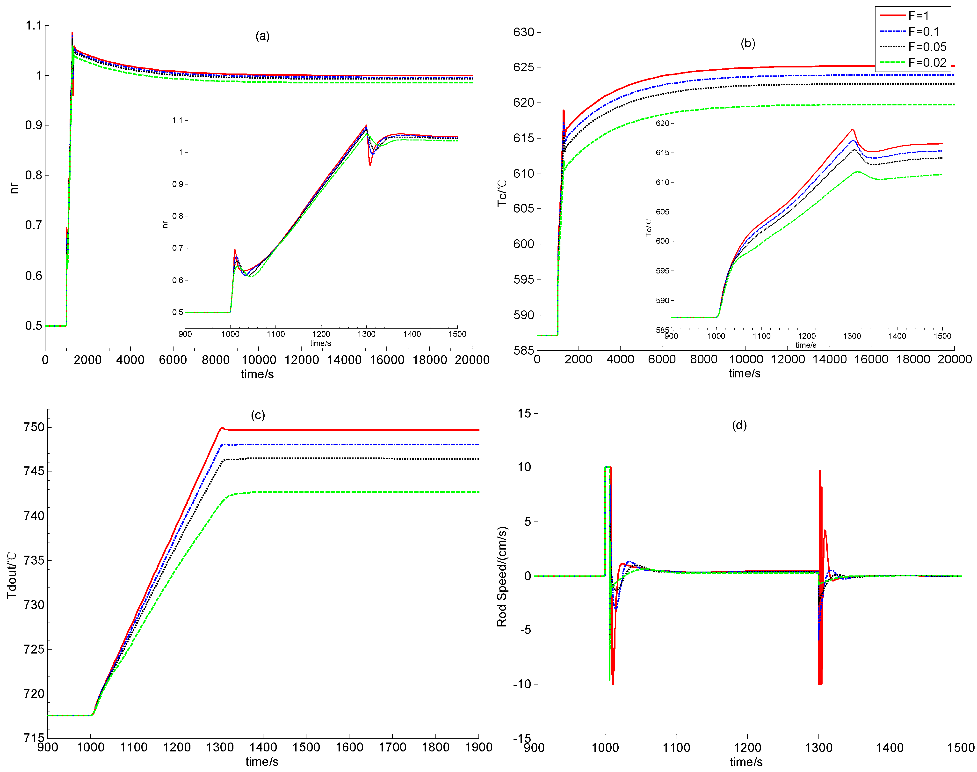
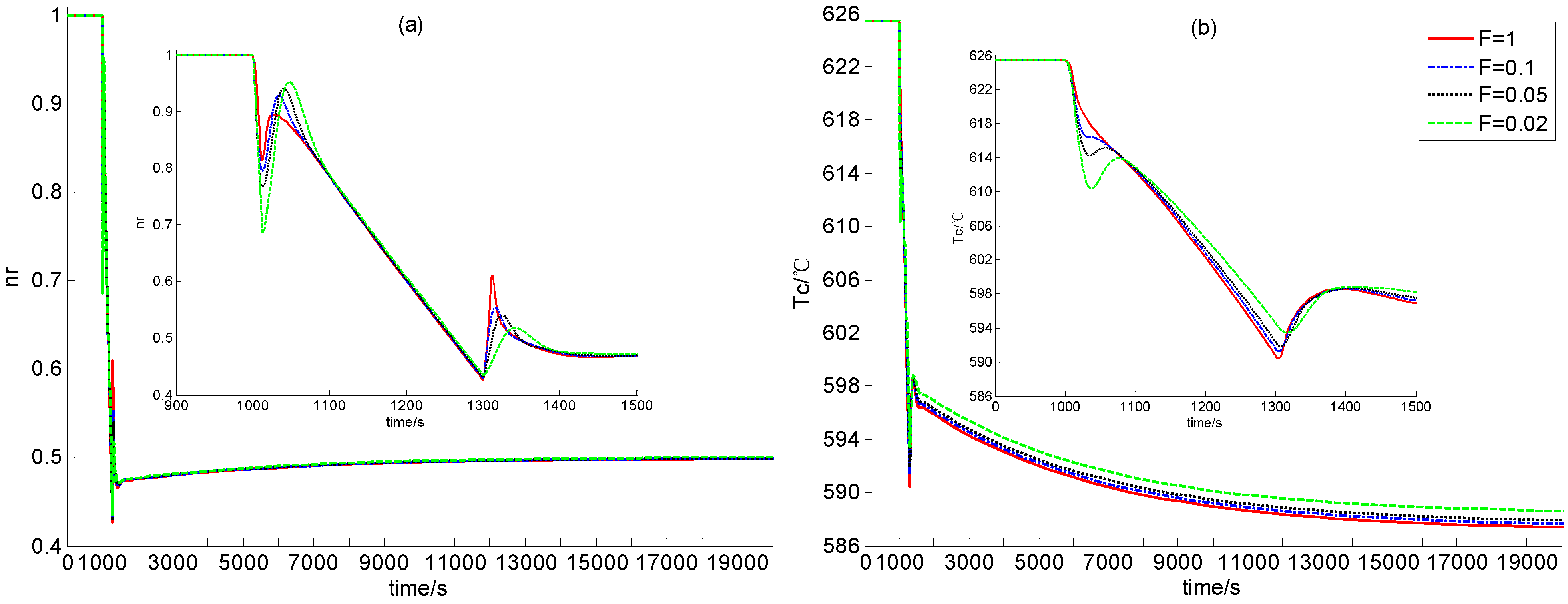
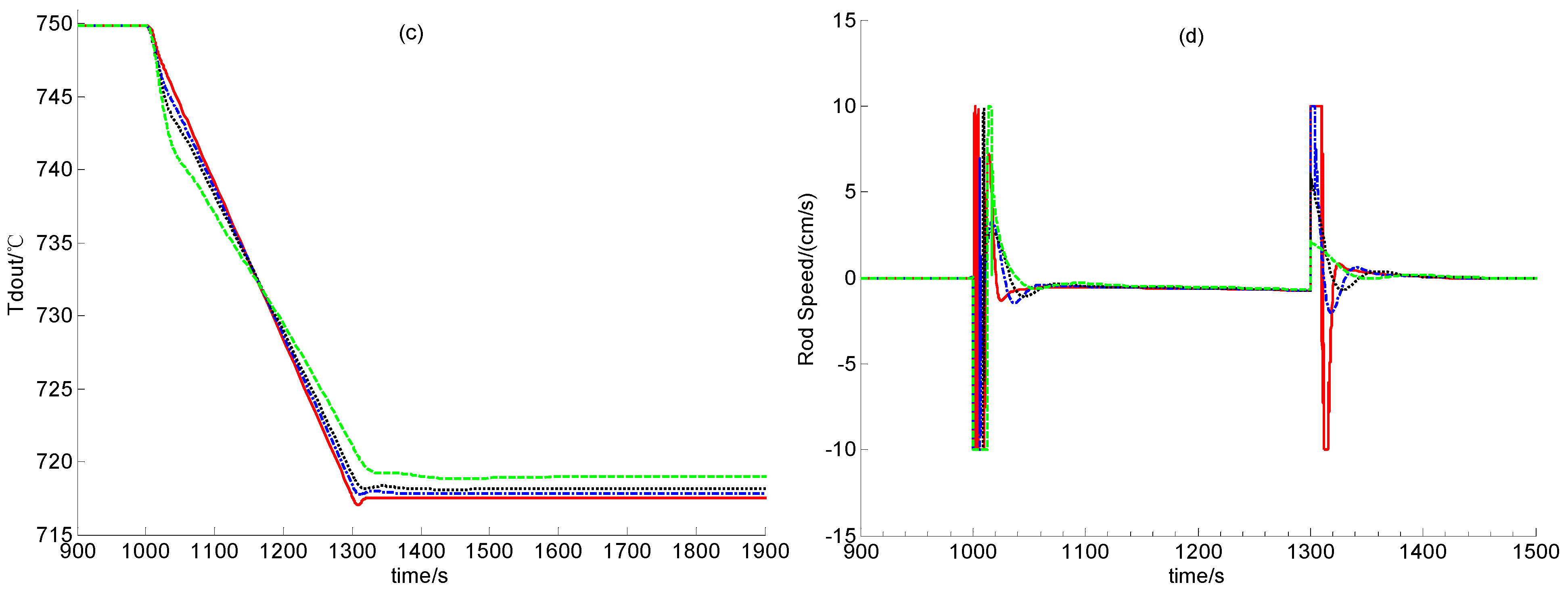
In this verification, the power demand decreases and increases linearly between 100% and 50% reactor full power-level (RFP). Due to the increase of the power demand from 50% to100% RFP, there are negative errors between the actual and set values of the nuclear power and the temperatures of the fuel, the helium flow and the reflector. These errors drive the power-level control strategy to lift the control rods for weakening these error signals. The transient responses of the relative nuclear power, the average fuel temperature, the outlet helium temperature and the control rod speed signal are all illustrated in Figure 4. As the power demand signal decreases from 100% to 50% RFP, there must be positive errors between the actual and set values of the process state variables which result in the insertion of control rods. The transient responses caused by the power demand decrease from 100% to 50% RFP are given in Figure 5.

Figure 4. Simulation Results in Case A1.

Figure 4. Simulation Results in Case A1.

Figure 5. Simulation Results in Case A2.

Figure 5. Simulation Results in Case A2.

Case B:

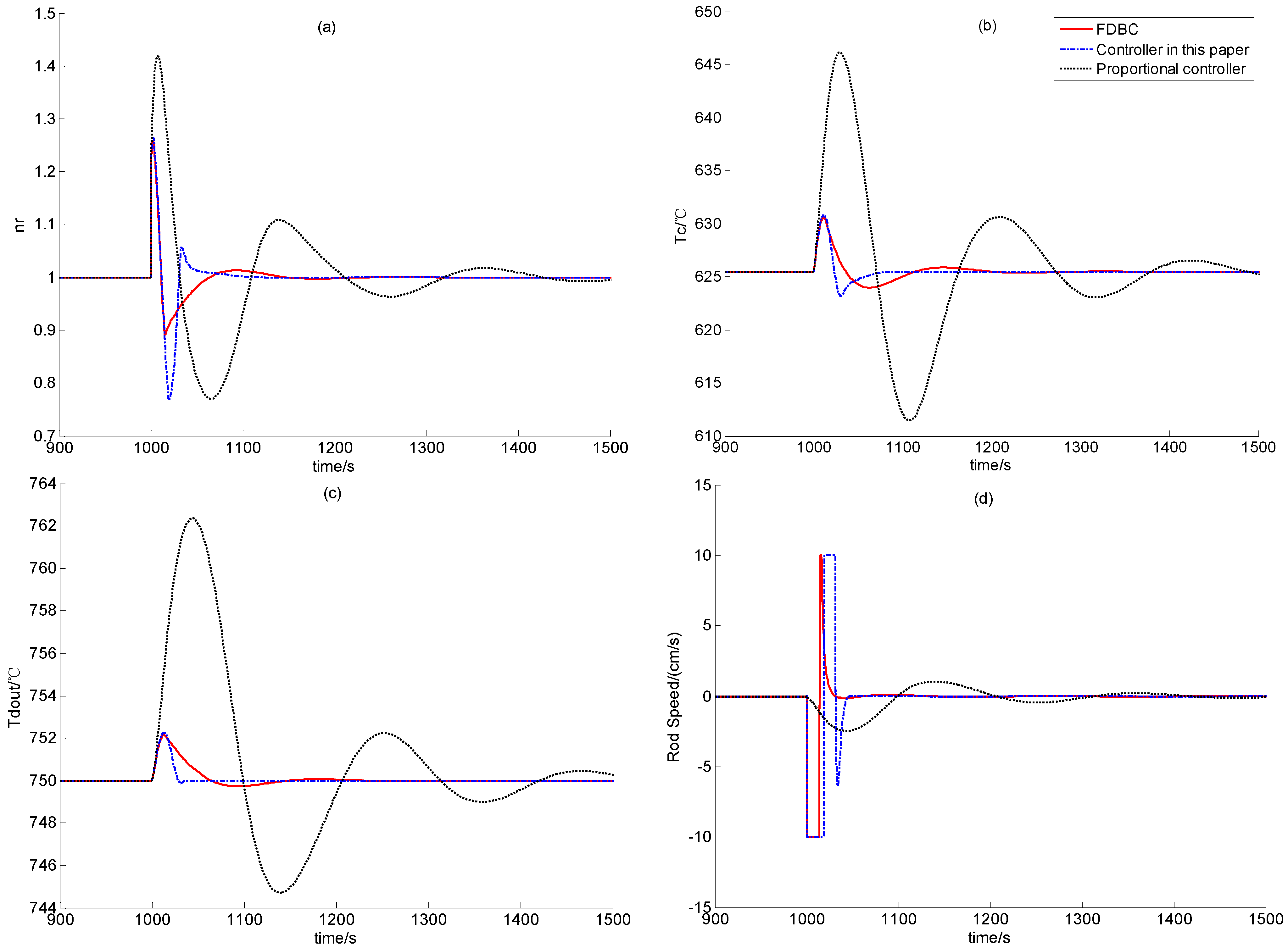
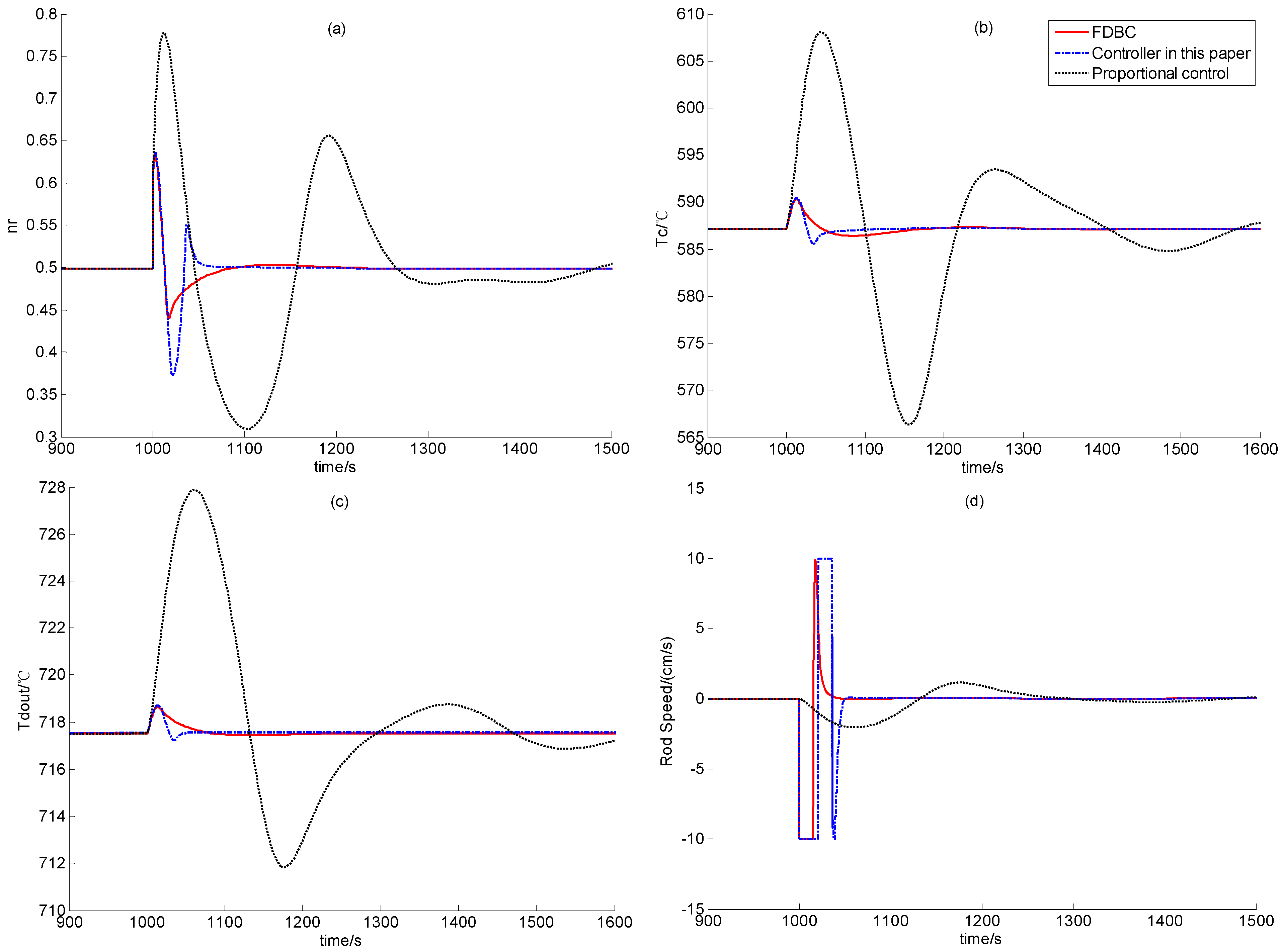
In this test, a step positive reactivity disturbance valued 0.2β is added when the reactor is steady at 50% RFP for 1,000 seconds. This positive set of reactivity disturbance caused the increase of the nuclear power, which in turn leads to the increase of the temperatures of the fuel, the helium inside the reactor and the reflector. The transient responses of the process variables corresponding to the FDBC, controller (59) and simple proportional controller (82) are all shown in Figure 6. The simulation results at 100% RFP with the same step positive reactivity disturbance are shown in Figure 7.

Figure 6. Simulation Results in Case B1.

Figure 6. Simulation Results in Case B1.

4.2. Discussion

The power demand increase leads δn_r to be negative and decreasing, which drives the power-level controller to generate a positive control rod speed signal. This results in the increases of both the neutron concentration and the fuel temperature. The heated fuel elements provide the increase of the outlet helium temperature. The reactor enters a steady state if the reactivity caused by the temperature feedback effect cancels that induced by withdrawing the control rods. Similarly, the power demand decrease results in a positive and increasing δn_r, which drives the control law to insert the control rods. This operation makes the neutron concentration, the fuel temperature and the outlet helium temperature decrease all. The entire system comes into a steady state if the reactivity given by the temperature feedback cancels that caused by inserting the control rods.

From Figure 4 and Figure 5, the newly-built power level control provides satisfactory regulation performance in cases of the power decrease and the power increase if scalar F is large enough. This shows the strong feasibility of this newly-built dynamic output power-level control law. Moreover, from Figure 4 and Figure 5, if F is smaller, i.e., if both observer gains F₁ and F₂ are smaller, then steady control error is larger. This is because that the observer gains are smaller, the L₂ gain from the disturbance to the evaluation signal is larger, which means that the modeling error between the dynamic model for control design and that for simulation leads to larger regulation error, as we can see from Figure 4 and Figure 5.

Figure 7. Simulation Results in Case B2.

Figure 7. Simulation Results in Case B2.

From the performance comparison results illustrated by Figure 6 and Figure 7, a simple proportional feedback controller leads to extensive large overshoot and quite long transition period, and the FDBC has the best disturbance attenuation performance. Since the FDBC has the feedback loops of both the nuclear power and helium temperature, its performance is surely the best. However, though the control law developed in this paper only has the feedback loop of the helium temperature, its performance is very close to that of the FDBC, and the transition period of this newly-built controller is even smaller than that of the FDBC. This is mainly because observer (10) provides enough good state-observation for recover the performance of globally asymptotic stabilizer IDA-PLC presented in [14].

Finally, from the simulation results and the above discussion we can see that the performance of the newly-built power-level control strategy, using only with helium temperature feedback loop, is satisfactory, and the application of this new control law to a practical engineering scenario is feasible. Especially when the sensor of the neutron concentration is in error, the dynamic output feedback control law proposed in this paper can maintain the control performance.

5. Conclusions

Power-level control techniques are crucial for the safe, stable and efficient operation of any nuclear reactor, including MHTGRs. The current power-level control laws for nuclear reactors mostly rely on the measurement of both the nuclear power and the coolant temperature. However, if the neutron sensors are in error, these control strategy cannot provide satisfactory performance, and may even cause extensive overshoots of the process variables. Since the inlet and outlet coolant temperatures are relatively easy to measure, it is meaningful to design power-level controllers only with the feedback loop of the coolant temperature. Furthermore, this type of power-level controller is also meaningful to those pebble-bed MHTGRs for regulating the total reactor thermal power in the phases of loading or unloading fuel elements. It is also clear that a state-observer only needing the measurement of the coolant temperature is key for develop this type of power-level controller. Stimulated by this, a novel nonlinear state-observer is established for the MHTGRs in this paper. It has been proven that this observer is globally convergent if there is no disturbance, and has the L₂ disturbance attenuation performance if the disturbance is nonzero. Moreover, the separation principles of this observer are also proved, which denotes that this observer can cover the performance of the globally asymptotic stabilizer and the L₂ disturbance attenuator. Then a dynamic output feedback power-level control strategy is formed by this new observer and the IDA-PLC presented in [14]. Finally numerical simulation results are given to verify the feasibility of the newly-built controller. The simulation results in case of power maneuver show that the performance of this newly-built dynamic output feedback power-level controller can be satisfactory if the observer feedback gains are high enough. Moreover, this new control has also been compared to the FDBC given in [13] and proportional feedback controller (82), which further shows the high performance and feasibility of this newly-developed power-level controller.

References

- Wu, Z.; Lin, D.; Zhong, D. The design features of the HTR-10. Nuclear Eng. Design 2002, 218, 25–32. [Google Scholar] [CrossRef]
- Hu, S.; Liang, X.; Wei, L. Commissioning and operation experience and safety experiment on HTR-10. In Proceedings of the 3rd International Topical Meeting on High Temperature Reactor Technology, Johannesburg, South Africa; 2006. D00000052. [Google Scholar]
- Zhang, Z.; Wu, Z.; Wang, D.; Xu, Y.; Sun, Y.; Li, F.; Dong, Y. Current status and technical description of Chinese 2 × 250 MWth HTR-PM demonstration plant. Nuclear Eng. Design 2009, 239, 1212–1219. [Google Scholar] [CrossRef]
- Zhang, Z.; Sun, Y. Economic potential of modular reactor nuclear power plants based on the Chinese HTR-PM project. Nuclear Eng. Design 2007, 237, 2265–2274. [Google Scholar] [CrossRef]
- Edwards, R.M.; Lee, K.Y.; Schultz, M.A. State-feedback assisted classical control: an incremental approach to control modernization of existing and future nuclear reactors and power plants. Nuclear Technol. 1990, 92, 167–185. [Google Scholar]
- Ben-Abdennour, A.; Edwards, R.M.; Lee, K.Y. LQR/LTR robust control of nuclear reactors with improved temperature performance. IEEE Trans. Nuclear Sci. 1992, 39, 2286–2294. [Google Scholar] [CrossRef]
- Arab-Alibeik, H.; Setayeshi, S. Improved temperature control of a PWR nuclear reactor using LQG/LTR based controller. IEEE Trans. Nuclear Sci. 2003, 50, 211–218. [Google Scholar] [CrossRef]
- Ku, C.-C.; Lee, K.Y.; Edwards, R.M. Improved nuclear reactor temperature control using diagonal recurrent neural networks. IEEE Trans. Nuclear Sci. 1992, 39, 2298–2308. [Google Scholar] [CrossRef]
- Shtessel, Y.B. Sliding mode control of the space nuclear reactor system. IEEE Trans. Aerosp. Electron. Syst. 1998, 34, 579–589. [Google Scholar] [CrossRef]
- Arab-Alibeik, H.; Setayeshi, S. Adaptive control of a PWR core power using neural networks. Ann. Nuclear Energy 2005, 32, 588–605. [Google Scholar] [CrossRef]
- Na, M.G.; Hwang, I.J.; Lee, Y.J. Design of a fuzzy model predictive power controller for pressurized water reactors. IEEE Trans. Nuclear Sci. 2006, 53, 1504–1514. [Google Scholar] [CrossRef]
- Eliasi, H.; Menhaj, M.B.; Davilu, H. Robust nonlinear model predictive control for a PWR nuclear power plant. Prog. Nuclear Energy 2012, 54, 177–185. [Google Scholar] [CrossRef]
- Dong, Z. Output feedback dissipation control for the power-level of modular high-temperature gas-cooled reactors. Energies 2011, 4, 1858–1879. [Google Scholar] [CrossRef]
- Dong, Z. Dynamic output feedback power-level control for the MHTGR based on iterative damping assignment. Energies 2012, 5, 1782–1815. [Google Scholar] [CrossRef]
- Dong, Z.; Feng, J.; Huang, X.; Zhang, L. Dissipation-based high gain filter for monitoring nuclear reactors. IEEE Trans. Nuclear Sci. 2010, 57, 328–339. [Google Scholar] [CrossRef]
- Dong, Z.; Huang, X.; Zhang, L. Output feedback power-level control of nuclear reactors based on a dissipative high gain filter. Nuclear Eng. Design 2011, 241, 4783–4793. [Google Scholar] [CrossRef]
- Li, H.; Huang, X.; Zhang, L. A simplified mathematical dynamic model of the HTR-10 high temperature gas-cooled reactor with control system design purpose. Ann. Nuclear Energy 2008, 35, 1642–1651. [Google Scholar] [CrossRef]
- Khalil, H. Nonlinear Systems, 3rd ed.; Prentice-Hall: Upper Saddle River, NJ, USA, 2002. [Google Scholar]
- Dong, Z.; Huang, X. Real-time simulation platform for the design and verification of the operation strategy of the HTR-PM. In Proceedings of the 19th International Conference on Nuclear Engineering (ICONE19), Chiba, Japan; 2011. ICONE19–44004. [Google Scholar]
- Dong, Z.; Huang, X.; Zhang, L. A nodal dynamic model for control system design and simulation of an MHTGR core. Nuclear Eng. Design 2010, 240, 1251–1261. [Google Scholar] [CrossRef]
- Li, H.; Huang, X.; Zhang, L. A lumped parameter dynamic model of the helical coiled once-through steam generator with movable boundaries. Nuclear Eng. Design 2008, 238, 1657–1663. [Google Scholar] [CrossRef]
© 2013 by the authors; licensee MDPI, Basel, Switzerland. This article is an open access article distributed under the terms and conditions of the Creative Commons Attribution license (http://creativecommons.org/licenses/by/3.0/).
Share and Cite
MDPI and ACS Style
Dong, Z. Nonlinear Power-Level Control of the MHTGR Only with the Feedback Loop of Helium Temperature. Energies 2013, 6, 1142-1164. https://doi.org/10.3390/en6021142
AMA Style
Dong Z. Nonlinear Power-Level Control of the MHTGR Only with the Feedback Loop of Helium Temperature. Energies. 2013; 6(2):1142-1164. https://doi.org/10.3390/en6021142
Chicago/Turabian StyleDong, Zhe. 2013. "Nonlinear Power-Level Control of the MHTGR Only with the Feedback Loop of Helium Temperature" Energies 6, no. 2: 1142-1164. https://doi.org/10.3390/en6021142