Analysis of Similarity Measures in Times Series Clustering for the Discovery of Building Energy Patterns

Abstract

Forecasting and modeling building energy profiles require tools able to discover patterns within large amounts of collected information. Clustering is the main technique used to partition data into groups based on internal and a priori unknown schemes inherent of the data. The adjustment and parameterization of the whole clustering task is complex and submitted to several uncertainties, being the similarity metric one of the first decisions to be made in order to establish how the distance between two independent vectors must be measured. The present paper checks the effect of similarity measures in the application of clustering for discovering representatives in cases where correlation is supposed to be an important factor to consider, e.g., time series. This is a necessary step for the optimized design and development of efficient clustering-based models, predictors and controllers of time-dependent processes, e.g., building energy consumption patterns. In addition, clustered-vector balance is proposed as a validation technique to compare clustering performances.

1. Introduction

The classification and modeling of buildings’ energy behavior is a core point to improve several emerging applications and services. For instance, the existence of databases with building energy profiles in connection with BIM models (Building Information Modeling) points out to be a key factor to achieve more sustainable building designs as well as more energy efficient urban development [1] (the more accurate and realistic energy profiles are, the better building energy performance calculations become).

A different but obviously related application area is the electricity market, which claims solutions and proposals that bestow flexibility on it. Expected enhancements must allow to smooth the frequent peaks and imbalances that are detrimental to all links in the energy chain, from suppliers to users [2]. Within this scope, demand or consumption habits can be abstracted by energy models that lead us to customized, more effective and fair relationships between energy providers and customers [3,4]. As further examples, energy use models are also found relevant to enhance the exploitation of renewable energy sources [5], or to achieve smart grid operation enhancement [6].

In the introduced scenarios, buildings—or buildings’ energy behaviors—are usually represented as time-based profiles or patterns to cluster. Indeed, the modeling and classification of building energy demand and consumption becomes one of the most representative application fields with regard to the clustering of time arranged data. As a general rule, in this scope clustering is commonly used to classify energy consumers [7], predict future energy demand [8,9], or detect distinguished, habitually undesired, behaviors (i.e., outliers) [10].

In addition to the purposes referred before, the identification of building energy patterns is also useful to provide context awareness capabilities to home and building control systems. Actually, the present work is motivated by the search of reliability and accuracy in the design of clustering-based controllers, models and predictors that operate with time-related information, which play a very important role in the fields of home and building automation, e.g., [11,12]. The selection of the building energy case is due to the wide scope of its application and the fact that the presented experiments could also be conducted with publicly available data.

Therefore, looking for the improvement of clustering-based applications, this paper develops a novel cluster validation method—clustered-vector balance—to be the basis of sensitivity analysis for the adjustment of clustering parameters, metrics and algorithms. The selected parameter under test is the similarity measure used to establish resemblance between two isolated samples, as it is a determining factor to assume in time series clustering. Since cluster validity methods also use similarity measures to check clustering solutions, the undertaken task is submitted to bias and uncertainty. The conducted experiments try to cope with such a problem performing a set of tests where similarity distances for clustering, as well as for evaluation and validation, are repeatedly switched. In addition to cluster-vector balance, classic cluster validity techniques are also utilized, as well as evaluations using non-clustered data. The cross comparisons let us infer some hypothesis related to the usage of the selected similarity measures for model discovery in univariate time series clustering.

2. Embedding Clustering in Real Applications

The application of clustering or cluster analysis usually covers one or more of the following aims: data reduction, hypothesis generation, hypothesis testing or prediction based on groups [13]. Indeed, the problem scenario that clustering has to face can take thousands of different shapes, but they usually share a common problem description: given a certain amount of input data vectors, characterized by a set of features or variables, an unsupervised knowledge abstraction of the data is required in order to allow its classification and representation.

It means that we always begin from certain ignorance concerning how the available or potential set of data can be internally arranged or structured. On the other hand, clustering adjustment and parametrization demand a deep understanding of the problem nature and domain in order to overcome several significant uncertainties [14]. Otherwise, the blind application of clustering techniques leads to trivial, erroneous or inefficient solutions. Therefore, the more previous knowledge about the nature of data exists, the better the clustering solution will be. As you can see, it entails a certain circularity that emphasizes the complex background of clustering.

There are several works intended to support the design of clustering-based applications (e.g., [15]). In addition, it is rather common that the continuous refinement of such applications leads practitioners to progressively reach some better knowledge of the data nature, being hypothesis generation an almost unavoidable companion in the careful design of clustering-based processes.

Some of the difficulties or uncertainties to face in the clustering task involve the selection and adjustment of clustering criteria, clustering algorithms, initial number of clusters, the most suitable features, outlier definition and handling, proximity measures, validation techniques, etc. Among them, a basic question remains in the proximity measure, i.e., similarity or resemblance between two independent vectors. Euclidean distance is de facto the most applied similarity metric and usually appropriate for applications that do not present directly or necessarily correlation among distinct features. However, time series clustering deploys vectors where the information are time arranged, thus considering correlation in the similarity measures points out to be suitable, or better, even leading to more accurate solutions.

3. Clustering for Pattern Discovery in Time Series

The task of clustering time series for pattern discovery has the aim to find out a set of model profiles or patterns that represent as faithfully as possible the original data set, in a way that every independent vector of this original data can be considered as one of the models submitted to acceptable deviations or drifts, or an outlier at the most.

The difference between time series and normal clustering is that, in the time series case, the shape of input vectors entails features that are arranged in time. Hence, in univariate time series an input vector is usually the succession of values that a certain variable takes throughout a specific time scope.

Clustering time series is usually tackled twofold: (a) feature-based or model-based, i.e., previously summarizing or transforming raw data by means of feature extraction or parametric models, e.g., dynamic regression, ARIMA, neural networks [16]; so the problem is moved to a space where clustering works more easily; (b) raw-data-based, where clustering is directly applied over time series vectors without any space-transformation previous to the clustering phase. Several works concerning each kind of time series clustering are referred to in detail in [17].

Beyond the obvious loss of information due to feature-based or model-based techniques, they can also present additional drawbacks; for instance, the application-dependence of the feature selection, or problems associated to parametric modeling. On the other hand, characteristic drawbacks of raw-data-based approaches are: working with high-dimensional spaces (curse of dimensionality [18]), and being sensitive to noisy input data.

In any case, we focus on the raw-data-based option for two reasons: (1) conclusions and hypothesis can be more easily generalized for other behaviour modeling applications (e.g., individual or community profiles for energy, occupancy, comfort temperature, etc.); (2) this is the best option to clearly analyze correlated data in clustering. Indeed, selecting the correct distance measure able to evaluate correlation is the main difficulty in this kind of time series clustering.

4. Similarity Measures

We consider similarity as the measure that establishes an absolute value of resemblance between two vectors, in principle isolated from the rest of the vectors and without assessing the location inside the solution space.

Considering continuous features, the most common metric is the Euclidean distance:

$$d_E(\overrightarrow{x},\overrightarrow{y})=\sqrt{(\overrightarrow{x}-\overrightarrow{y}){(\overrightarrow{x}-\overrightarrow{y})}^{\prime }}$$

(1)

Note that Euclidean distance is invariant when dealing with changes in the order that time fields/features are presented; it means that it is in principle blind to capture vector or feature correlation. For time series data comparison, where trends and evolutions are intended to be evaluated, or when the shape formed by the ordered succession of features (i.e., the envelope) is relevant, similarity measures based on Pearson’s correlation:

$$d_C(\overrightarrow{x},\overrightarrow{y})=1-\frac{(\overrightarrow{x}-\overline{\overrightarrow{x}}){(\overrightarrow{y}-\overline{\overrightarrow{y}})}^{\prime }}{\sqrt{(\overrightarrow{x}-\overline{\overrightarrow{x}}){(\overrightarrow{x}-\overline{\overrightarrow{x}})}^{\prime }}\sqrt{(\overrightarrow{y}-\overline{\overrightarrow{y}}){(\overrightarrow{y}-\overline{\overrightarrow{y}})}^{\prime }}}$$

(2)

have also been widely utilized, although it is not free of distortions or problems [19]. Mahalanobis distance,

$$d_M(\overrightarrow{x},\overrightarrow{y})=\sqrt{(\overrightarrow{x}-\overrightarrow{y})C^{-1}{(\overrightarrow{x}-\overrightarrow{y})}^{\prime }}$$

(3)

can be seen as an evolution of the Euclidean distance that takes into account data correlation. It utilizes the covariance matrix of input vectors C for weighting the features. Mahalanobis distance usually performs successfully with large data sets with reduced features, otherwise undesirable redundancies tend to distort the results [20].

An interesting measure specially addressed to time series comparison is the Dynamic Time Warping (DTW) distance [21]. This measure allows a non-linear mapping of two vectors by minimizing the distance between them. It can be used for vectors of different lengths: $\overrightarrow{x}=x_1,...,x_i,...,x_n$ and $\overrightarrow{y}=y_1,...,y_j,...,y_m$. The metric establishes an n-by-m cost matrix C which contains the distances (usually Euclidean) between two points $x_i$ and $y_j$. A warping path $W=w_1,w_2,...,w_K$, where $\max (m,n)\le K<m+n-1$, is formed by a set of matrix components, respecting the next rules:

• Boundary condition: $w_1=C(1,1)$ and $w_K=C(n,m)$;
• Monotonicity condition: given $w_k=C(a,b)$ and $w_{k-1}=C(a^{\prime },b^{\prime })$, $a\ge a^{\prime }$ and $b\ge b^{\prime }$;
• Step size condition: given $w_k=C(a,b)$ and $w_{k-1}=C(a^{\prime },b^{\prime })$, $a-a^{\prime }\le 1$ and $b-b^{\prime }\le 1$.

There are many paths that accomplish the introduced conditions; among them, the one that minimizes the warping cost is considered the DTW distance:

$$d_W(\overrightarrow{x},\overrightarrow{y})=\min \left(\sqrt{{\displaystyle \sum _{k=1}^K{w}_k}}\right)$$

(4)

The main drawback of the measure remains in the effort dedicated to the calculation of the path of minimal cost, in addition to the fact that, actually, it cannot be considered as a metric, i.e., it does not accomplish the triangular inequality.

In the current work, we focus on these four general-purpose popular distances, in spite of the fact that there exist many additional similarity measures. A survey of distance metrics for time series clustering can be found in [17]. Other noteworthy options are the cosine measure [22], which is good for patterns with different or variable size or length; or Jaccard and Tanimoto similarity measures, that can also be intuitively understood as a combination of Euclidean distances and correlations assessed by means of the inner product [23].

5. Cluster Validation

We can say that the validation of the results obtained by a clustering algorithm tries to give us a measure about the level of success and correctness reached by the algorithm. Here, we differentiate two ways of checking clustering solutions:

• On one hand, we have cluster validity or clustering validation methods, which try to evaluate results according to mathematical analysis and direct observation of solutions based on the inherent characteristics owned by the input data set. In a way of speaking, it consists of idealistic analysis methods as they focus on the definition given to a cluster irrespective of the reason that lead us to deploy clustering (i.e., the final application);
• On the other hand, sometimes clustering solutions can be benchmarked and checked directly by the application or an environment that simulates the application (entitled clustering evaluation). It is a practical (or engineering) approach, which mainly covers application-based tests. Here, generalizations are riskier; note that we carry corruption and deformations introduced by the application, the boundary conditions and the specific data used for testing.

In both cases, the value of such quantitative measures is always relative, it means that they “are only tools at the disposal of the experts in order to evaluate the resulting clustering” [13].

With regard to clustering validation, three different kinds of criteria are usually considered: external criteria, evaluations of how the solution matches a pre-defined structure based on a previous intuition concerning the data nature (e.g., the adjusted Rand index [24]); internal criteria, which evaluate the solution only considering the quantities and relationships of the vectors of the data set (e.g., proximity matrix); and relative criteria, carried out comparing clustering solutions where one or more parameters have been modified (e.g., cluster silhouettes [25]).

In [26], some of these validation methods are introduced, concluding that they usually work better when dealing with compact clusters. This reasoning yields an interesting point that remarks the uncertainty also related to cluster validity; i.e., as it happens with clustering that usually imposes a structure on the input data, cluster validation methods also impose a rigid definition of what a good cluster is and develop their assessments according to this particular definition.

Uncertainties, commitments and discussions also appear concerning the foundations of the cluster validity measures, as they must fix some essential concepts. To refer some examples: how clusters must be represented, how to calculate the distance between two clusters, how to calculate the distance between a point and a cluster, or even which kind of metric must be used for the distance measurement. Beyond these aspects, there exists lot of work that compares clustering solutions by distinct techniques. To give some instances: in [27] clustering methods are benchmarked utilizing Log Likelihood and classification accuracy criteria. In [28], popular algorithms are analyzed from three different viewpoints: clustering criteria, or the definition of similarity; cluster representation and algorithm framework, which stands for the time complexity, the required parameters and the techniques of preprocessing. In [29] the criteria are mentioned “stability (Does the clustering change only modestly as the system undergoes modest updating?), authoritativeness (Does the clustering reasonably approximate the structure an authority provides?) and extremity of cluster distribution (Does the clustering avoid huge clusters and many very small clusters?)”.

6. Clustered-Vector Balance

In this paper, we start on the definition of clustering provided by [30], i.e., a group or cluster can be defined as a dense region of objects or elements surrounded by a region of low density. From here, a consequent step is to consider that any output group can be represented by a model individual (existent or nonexistent), which usually will correspond to the gravity center of the respective cluster, named centroid, discovered pattern, representative or model.

Our intended applications mainly use clustering for pattern or representative discovery, so we find suitable validity methods that focus on representativeness or give an important role to the representatives [31]. Therefore, we have developed a validity measure called clustered-vector balance (or simply vector balance) based on the clustering balance measurement introduced in [32]. The clustering balance measurement finds the ideal clustering solution when “intra-cluster similarity is maximized and inter-cluster similarity is minimized”. In order to extend the comparison to partitioning clustering with other parameters under test in addition to the number of clusters, we introduce substantial modifications to the original equations.

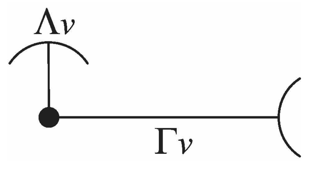
In the clustered-vector balance validation technique, every solution is expressed by a representative clustered-vector, which takes ${\Lambda }_v$ and ${\Gamma }_v$ (intra-cluster and inter-cluster average distance per vector) as component values (Figure 1). The expressions for ${\Lambda }_v$ and ${\Gamma }_v$ rest as follows:

$${\displaystyle {\Lambda }_v=\frac{1}{n}\sum _{j=1}^k\sum _{i=1}^{n_j}e(p_i^{(j)},p_0^{(j)})}$$

(5)

Figure 1. Symbol for a representative clustered-vector. The short segment with the concave arc stands for the average intra-cluster distance, the long segment with the convex arc for the average inter-cluster distance.

Figure 1. Symbol for a representative clustered-vector. The short segment with the concave arc stands for the average intra-cluster distance, the long segment with the convex arc for the average inter-cluster distance.

$${\displaystyle {\Gamma }_v=\frac{1}{k(k-1)}\sum _{j=1}^k\frac{n_j}{n}\sum _{l\ne j}^{k}e(p_0^{(j)},p_0^{(l)})}$$

(6)

where n is the total number of input vectors, $n_j$ stands for the vectors embraced in cluster j and k is the number of clusters. $p_i^{(j)}$ refers to the input vector i that belongs to cluster j, whereas $p_0^{(j)}$ is the centroid or representative of cluster j. $e(\overrightarrow{x},\overrightarrow{y})$ stands for the error function or distance between the vectors $\overrightarrow{x}$ and $\overrightarrow{y}$. Note that the subindex v denotes the postscript “per vector”.

The main differences with respect to [32] remain in the definition of Γ, which now is not related to the distance to an hypothetical global centroid, but to the distances among centroids, individually weighted according to each cluster population. In addition, Λ and Γ are now expressed in connection with a single, representative vector for the whole solution, and this makes both magnitudes comparable. Therefore, ${\Lambda }_v$ is the average distance between a clustered vector and its centroid, whereas ${\Gamma }_v$ is the average distance between a clustered vector to other clusters (more specifically, to other centroids).

Directly relating ${\Lambda }_v$ and ${\Gamma }_v$ can lead to doubtful, meaningless absolute indexes. In [32], authors introduce an α weighting factor to achieve a commitment between Λ and Γ. The parameter seems to be arbitrarily defined just to relate to both indexes, being adjusted to $1/2$ by default without providing an appropriate discussion. In our case, we can obviously expect that the best solutions will tend to show lower ${\Lambda }_v$ and higher ${\Gamma }_v$, but the relationships among both values, their possible increments and the performance evaluation are not linear and have a high scenario-dependence. Since we lack a priori additional knowledge, the final clustered-vector balance index is proposed to be obtained by relating ${\Lambda }_v$ and ${\Gamma }_v$ using a previous Z-score transformation (i.e., $z=\frac{x-\mu }{\sigma }$). Means and standard deviations of both ${\Lambda }_v$ and ${\Gamma }_v$ are obtained considering the total set of solutions to compare. Finally, the best solution maximizes:

$${\mathcal{E}}_v(\mathcal{X})={\Gamma }_{v_z}-{\Lambda }_{v_z}$$

(7)

We no longer require α. However, we can consciously add it again if we have a previous biased opinion with respect to what a good clustering solution is according to the final application, i.e., whether we want to favor solutions where clusters are compact or we prefer that they are as different/far as possible. Hence it would remain:

$${\mathcal{E}}_v(\mathcal{X})=\alpha {\Gamma }_{v_z}-(1-\alpha ){\Lambda }_{v_z}$$

(8)

7. Experiments

The conducted experiments have two main objectives:

• To check clustered-vector balance as a clustering validity algorithm by means of comparisons with other relative clustering validity criteria;
• To obtain a precedent for the selection of the most appropriate similarity metric for our application case—building energy consumption pattern discovery—which is a significant use case of time series clustering.

To do that, real cases are clustered using different similarity distances. Later on, each clustering solution is validated by means of different validation techniques (the similarity measure of the validation algorithm is switched as well). In addition, test vectors (selected at random and not processed by the clustering tool) are utilized to evaluate the representativeness of the main patterns of the cluster or centroids, measuring the average distance between the test vectors included in a cluster and the representative of the respective cluster [Equation (9)]. The evaluation also uses all of the diverse similarity distances under test.

$${\displaystyle V=\frac{1}{m}\sum _{j=1}^k\sum _{i=1}^{m_j}e(q_i^{(j)},p_0^{(j)})}$$

(9)

m is the total number of vectors put aside for evaluation, $m_j$ stands for the vectors embraced in cluster j. $q_i^{(j)}$ refers to the evaluation vector i that belongs to cluster j. The membership of the evaluation vectors is established according to the proximity to the found patterns $p_0$. e represents the distance used for evaluation.

In the trivial situation that all similarity measures affect the clustering solution in the same way, or in the hypothetical case that each distance is the most successful at finding a clustering solution with specific characteristics, we should expect that clustering carried out using a specific distance obtains the best results when the same distance has been used for validations or evaluations. Otherwise, we will have arguments to establish better and worse similarity measures for our specific application case.

7.1. Database

For the experiments, information concerning energy consumption of five university buildings has been collected. The buildings are located in Barcelona, Spain, and data cover hourly consumption from 29 August 2011 to 1 January 2012. Data is publicly available in (http://www.upc.edu/sirena). The selected buildings belong to the “Campus Nord”, they are: “Edifici A1”, “Edifici A4” and “Edifici A5” (university classrooms and laboratories), “Biblioteca” (a library) and “Rectorat” (an office building for administration and rectorship). In Table 1 and Figure 4, Figure 5 and Figure 6, B1, B2, B3, B4 and B5 identify the presented buildings in the introduced order. The usable spaces of the buildings have the following dimensions: B1, 3966.59 m${}^2$; B2, 3794.95 m${}^2$; B3, 3886.12 m${}^2$; B4, 6644.4 m${}^2$; B5, 5927.21 m${}^2$.

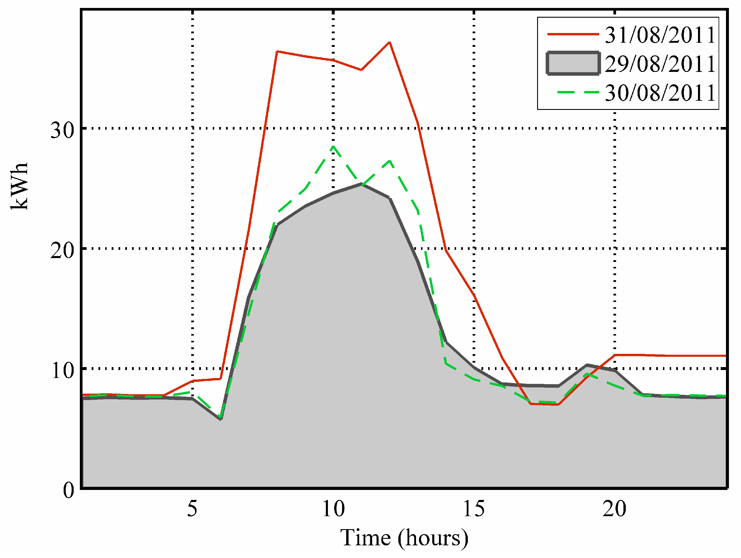
Each building presents 124 days of information, 100 days taken for training and for the cluster validity analysis, and 24 days employed in the evaluation. Input vectors are time series with 24-fields of hourly information concerning the energy consumption in kWh (Figure 2).

Figure 2. Example of three consecutive consumption days (“Rectorat”).

Figure 2. Example of three consecutive consumption days (“Rectorat”).

Analysis prior to the clustering processes confirms notable data correlations in all the buildings. Table 1 displays, for each building, statistical data concerning correlation. Taking a daily profile at random, the values of the table show the number of other daily profiles of the same database with which the selected profile will present a Pearson’s correlation index higher than $0.8$ on average.

Table 1. Given a building, evaluation of the number of daily profiles ($\overline{x}\pm {\sigma }_x$) that keep $c\ge 0.8$ (Pearson’s correlation index) with a daily profile selected at random.

B1	B2	B3	B4	B5
$28.0\pm 22.3$	$31.2\pm 23.0$	$20.6\pm 15.9$	$81.6\pm 36.1$	$47.0\pm 18.1$

Table 1. Given a building, evaluation of the number of daily profiles ($\overline{x}\pm {\sigma }_x$) that keep $c\ge 0.8$ (Pearson’s correlation index) with a daily profile selected at random.

B1	B2	B3	B4	B5
$28.0\pm 22.3$	$31.2\pm 23.0$	$20.6\pm 15.9$	$81.6\pm 36.1$	$47.0\pm 18.1$

7.2. Tests and Parameters

The similarity measures under test have been explained in Section 4, they are: (a) Euclidean distance, (b) Mahalanobis distance, (c) distance based on Pearson’s correlation and (d) DTW distance. In the first step, the training data is processed by a Fuzzy clustering module that uses the FCM algorithm to compute clusters. As referred to above, the FCM algorithm uses the four distance measures to state vector proximity. In each case, the initial number of clusters has been fixed according to clustering balance and Mountain Visualization [33], as well as maintaining the final scenario purposes (i.e., allowing a maximum of 8 energy consumption models).

Since all features correspond to the same phenomenon (electricity consumption), normalization is not carried out feature by feature, but based on the mean μ and standard deviation σ of the whole dataset (i.e., a simple uniform scaling). Failing to ensure that all features move within similar ranges has been addressed as a problem for similarity measures like Euclidean distance, as “features with large values will have a larger influence than those with small values” [34]. In any case, for univariate time series we are confident that the multi-dimensional input space is not distorted and the relationship among features keep the same shape and proportionality.

The clustering solutions are validated using: (a) clustering balance with $\alpha =1/2$ [32], (b) clustered-vector balance (Section 6), (c) Dunn’s index [35], (d) Davies–Bouldin index [36], and evaluated by means of (e) Equation (9), which checks how representative discovered patterns are by means of data separated for testing.

Therefore, the test process results in: $5\mathrm{builds.}\times 4\mathrm{clust.}(\mathrm{metrics})\times 4\mathrm{indices}\times 4\mathrm{index}(\mathrm{metrics})=320\mathrm{validations/evaluations}$. With all the obtained outcomes the next comparisons are carried out: (a) best clustering solution (best validation), (b) best evaluation, (c) soundness of validation algorithms, and (d) best independent clusters.

The last point refers to the capability of finding good clusters (i.e., dense, regular high similarity) irrespective of the global solution. The best clusters obtain minimum values in the next fitness function:

$$f_j=(1-m_j)\times {\Lambda }_j$$

(10)

where $m_j$ stands for the membership or amount of population embraced by cluster j (0: none; 1: all input samples) and ${\Lambda }_j$ for the intra-similarity of cluster j. Clusters must overcome a membership threshold to be taken into account ($m_j\ge 0.08$, i.e., at least $8\%$ of total population). This limit is a trade-off value established according to the application purposes, which requires a minimum level of representativeness for the discovered patterns.

8. Results

The high number of generated indices leads us to condense results in a meaningful way in some figures and tables. We discuss the obtained findings in separated points.

8.1. Characteristics of the Scenario Under Test

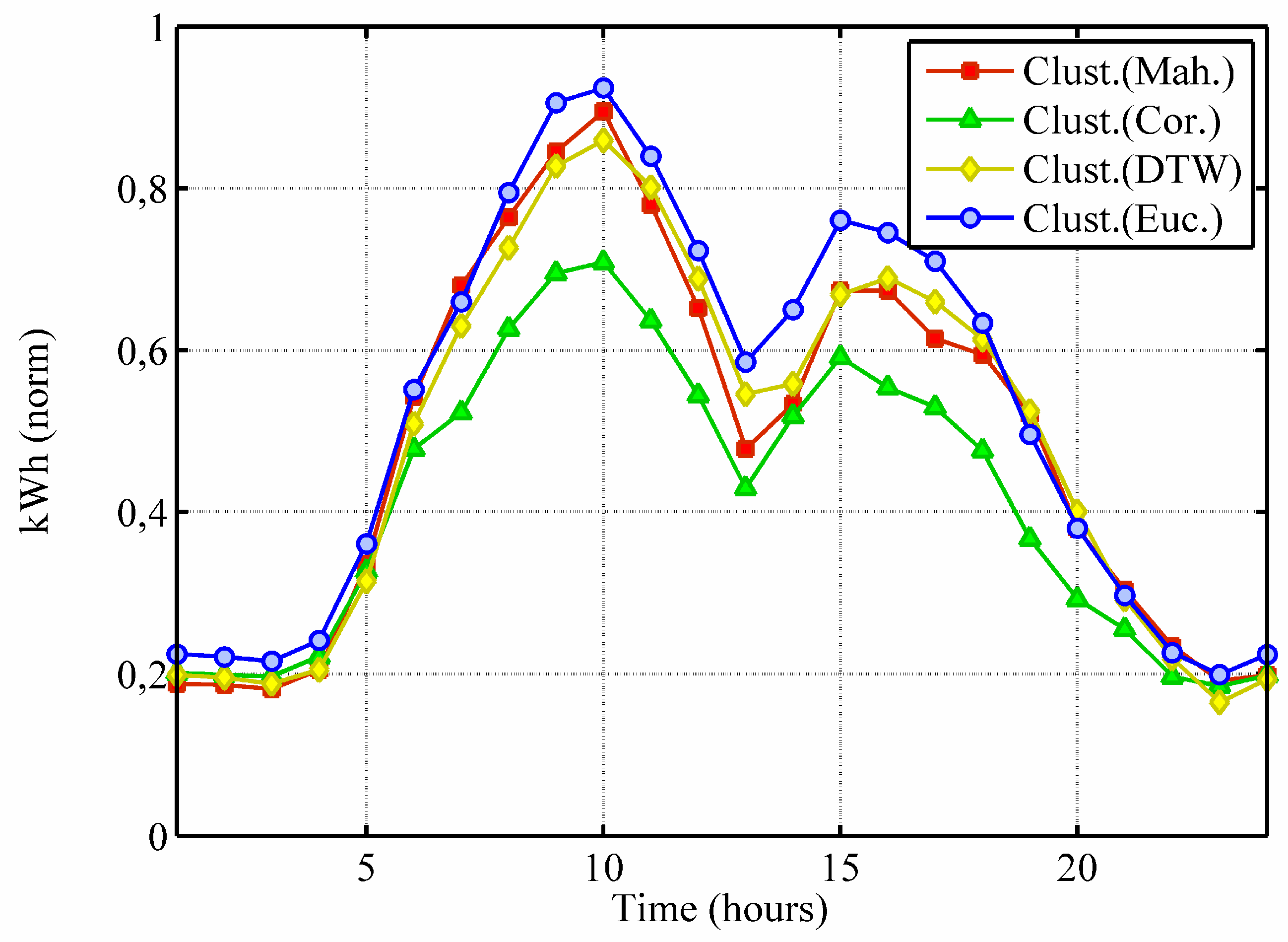
Experiments face quite a demanding scenario where to identify clear clusters is not an easy task and the selection of the similarity measure affects the shape of obtained models. It is obvious when the solution patterns are compared, e.g., Figure 3 shows the representative pattern corresponding to a specific discovered cluster according to every one of the clustering solutions in the case of building “Edifici A1”. Note that patterns are similar in shape, but different enough to have a relevant influence in subsequent applications. For instance, a control system that uses the predicted patterns to adjust the supply of energy sources in advance would perform differently in each case, resulting in distinct levels of costs and resource optimization. Moreover, the patterns displayed in the figure represent a different percentage of the input population (Euclidean: 17%, Mahalanobis: 20%, Correlation: 13%, DTW: 24%).

In addition, the demanding nature of the problem is also noticeable in the disagreement detected by the validation techniques (see next point).

Figure 3. Representative pattern of a specific cluster for building “Edifici A1” according to every clustering solution: using Euclidean (blue circles), Mahalanobis (red squares), based on Pearson’s Correlation (green triangles) and DTW (yellow diamonds) similarity metrics.

Figure 3. Representative pattern of a specific cluster for building “Edifici A1” according to every clustering solution: using Euclidean (blue circles), Mahalanobis (red squares), based on Pearson’s Correlation (green triangles) and DTW (yellow diamonds) similarity metrics.

8.2. Best Validation and Best Evaluation

To establish which similarity measure involves the best clustering performances, we must check all the tests together but separate validation from evaluation due to the different nature with which they approach the assessment task (see above).

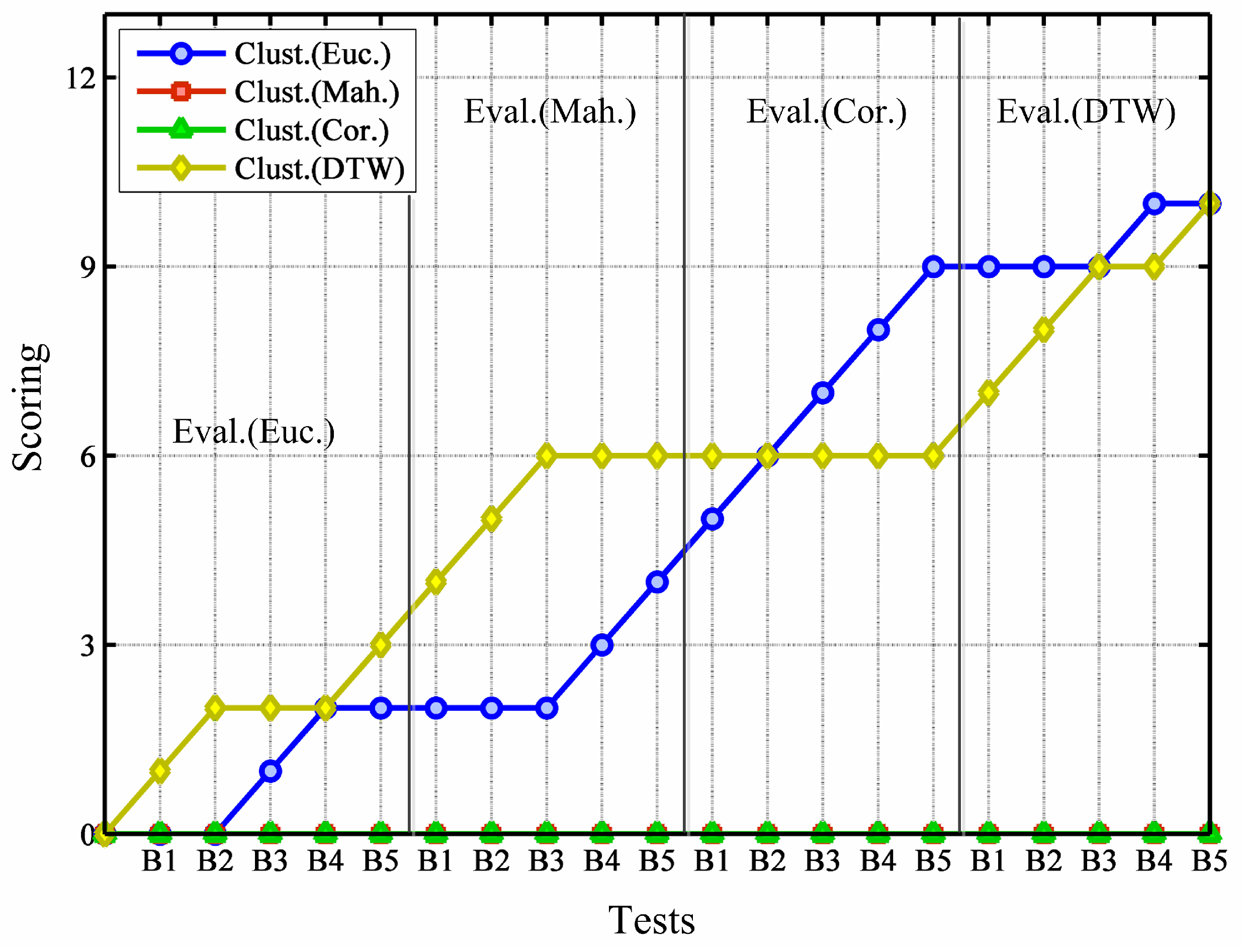
For the evaluation, we use four different validity methods. In order to gain an overall, joined perspective of the obtained results and indices, we ensure that they (validity methods) assign points to the similarity distance that they consider the best for every conducted test for every test, each validity method gives 1/4 points). For example, in building “Rectorat” (B5), in the test where validity methods deploy DTW distance for validation last test in Figure 4), Dunn’s index and clustered-vector balance index find that the Euclidean metric is the best, whereas Davies–Bouldin’ index bets for Mahalanobis metric, and finally, clustering balance supports the solution based on the DTW distance. Hence, in this example the Euclidean metric gains $1/2=1/4+1/4$ points, Mahalanobis metric $1/4$, DTW distance also $1/4$ and 0 for Correlation. 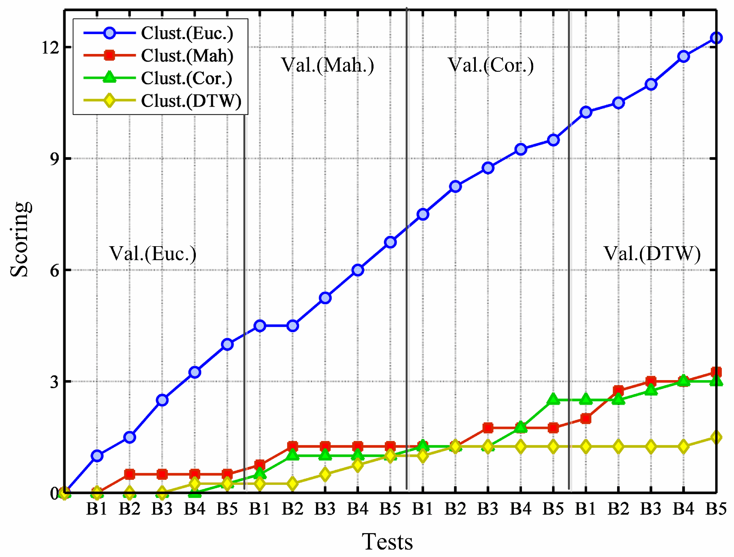This way of summarizing results leads to Figure 4. In the figure, tests are ordered from the building “Edifici A1” (B1) to the building “Rectorat” (B5), and starting with Euclidean metric for validation (left area), and finishing with DTW measure for validation (right area). In every test, the clustering solutions using the four different similarity measures are compared and points are given as described above.

What Figure 4 displays is that validity methods are prone to consider clustering solutions based on Euclidean metric as the best, irrespective of the measure used for validation. Moreover, note that the coincidence between the distance for clustering and the distance for validation has no significant influence in the assessments.

Figure 4. Joined assessment carried out by clustering validity methods.

Figure 4. Joined assessment carried out by clustering validity methods.

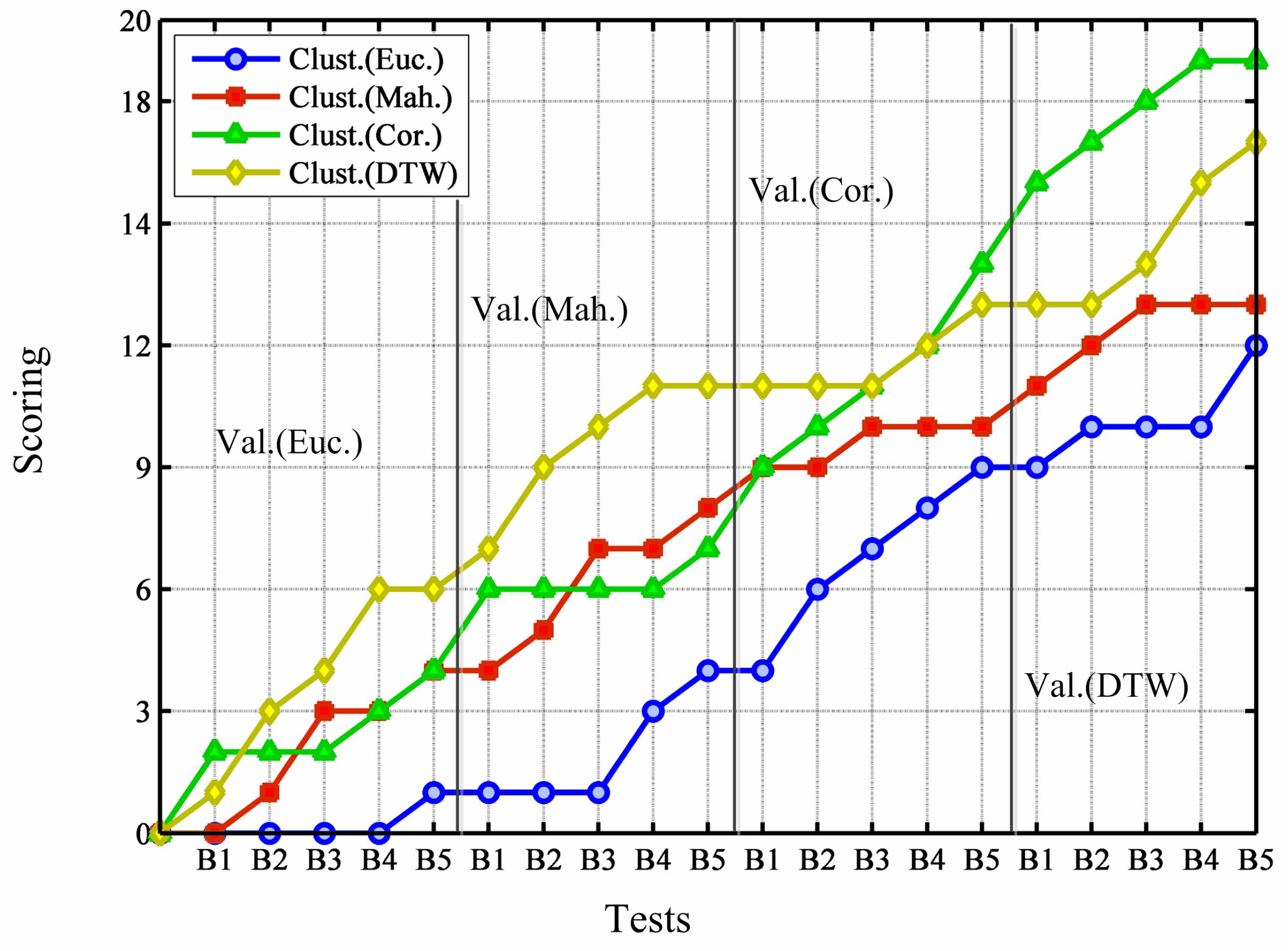
The case of validation is analogously checked, but here only Equation (9) is used for the assessments. Results are shown in Figure 5. Using data put aside for testing, evaluation reveals that DTW and Euclidean distances compete for the best scoring as measure of similarity for clustering, whereas Mahalanobis and Correlation metrics always perform worse. Curiously enough, DTW distance obtains the worst records in the validation analysis; this issue is dealt with later when validity methods are compared.

Figure 5. Assessment carried out using data saved for testing.

Figure 5. Assessment carried out using data saved for testing.

In short, as far as distances for clustering are compared, validation analysis set Euclidean as the best metric for time series clustering, whereas evaluation tests favor both DTW and Euclidean similarity distances.

8.3. Validation Algorithms

To review validation algorithms is not an easy task, note that the purpose here is to audit the performance of algorithms that are usually used for checking. In any case, we can reach some conclusions comparing their results to one another as well as looking at the evaluation outcomes. Table 2 displays the trends that validity techniques show when comparing clustering solutions that use different similarity measures. Considering all the tests together, the Mode represents the most typical position taken by the clustering solution that uses the marked distance, standing “1st” for the best evaluation and “4th” for the worst. The Mean contributes to the assessment and gives an impression about how stable the typical scoring is. Therefore, the next points can be reasoned from Table 2:

Table 2. Validity techniques evaluations, statistical Mode and Mean.

	Dunn	D-Boul.	Clust.b.	Vect.b.
	Mode – Mean	Mode – Mean	Mode – Mean	Mode – Mean
Clustering (Euclidean)	1st – 1.4	1st – 1.6	1st – 1.8	1st – 1.3
Clustering (Mahalanobis)	2nd – 2.3	3rd – 2.1	4th – 2.9	4th – 3.2
Clustering (Correlation)	3rd – 2.5	3rd – 2.5	4th – 3.0	4th – 3.2
Clustering (DTW)	4th – 3.9	4th – 3.9	3rd – 2.4	2nd – 2.4

Table 2. Validity techniques evaluations, statistical Mode and Mean.

	Dunn	D-Boul.	Clust.b.	Vect.b.
	Mode – Mean	Mode – Mean	Mode – Mean	Mode – Mean
Clustering (Euclidean)	1st – 1.4	1st – 1.6	1st – 1.8	1st – 1.3
Clustering (Mahalanobis)	2nd – 2.3	3rd – 2.1	4th – 2.9	4th – 3.2
Clustering (Correlation)	3rd – 2.5	3rd – 2.5	4th – 3.0	4th – 3.2
Clustering (DTW)	4th – 3.9	4th – 3.9	3rd – 2.4	2nd – 2.4

• All methods are in agreement over the measure that achieves the best clustering in general terms, i.e., Euclidean metric;
• Later on, two groups appear:

  –

  Group 1: Dunn’s and David–Bouldin’s indices usually scorn solutions based on DTW distance and put it in the worst place, finding that Mahalanobis and Correlation metrics are more suitable for the intended clustering;

  –

  Group 2: Otherwise, clustering balance and cluster-vector balance give credibility to the DTW distance, placing it before Mahalanobis and Correlation.

The validation tests favors the assessments given by Group 2, so we have arguments to believe that clustering balance and clustered-vector balance are techniques more appropriate to evaluate time series clustering solutions, at least for the current application case. If we look again at Table 2 and compare these two techniques with each other, vector balance seems to be more stable judging distance measures, whereas result comparisons of clustering balance are more variable and case-dependent. In short, there are three factors that opt for clustered-vector balance instead of clustering balance: clustered-vector balance (1) shows higher coincidence with the rest of validity methods, (2) is more stable in the assessments and (3) matches the validation test outcomes better.

Now it is possible to clarify why DTW distance gained such a low score in validation tests, in part due to the rejection of Dunn’s and David–Bouldin’s indices, but also because of the fact that, although usually showing a very little difference in the evaluations, clustered-vector balance rarely places DTW-based clustering before Euclidean-based (note that in Figure 4 and Figure 5 only the 1st solution obtains points; the 2nd, 3rd and 4th solutions gain no points).

8.4. Best Independent Clusters

Grouping all the clusters generated by the diverse clustering solutions together, the three best clusters according to Equation (10) are highlighted. Again a competition among similarity measures is carried out, and results are displayed in Figure 6. Here, results show no evidence to state that a specific distance measure obtains better compact clusters as a general rule. Again, the type of distance for validation does not significantly affect this measure (except for perhaps the case of Euclidean clustering); instead, the specific case (building) exerts a decisive influence for the selection of the measure to discover compact clusters (low internal dissimilarity). In any case, although results are not discriminative, it is at least worth considering the advantage of DTW and Correlation distances, and the fact that Euclidean metrics receives the lowest results in this aspect.

Figure 6. Comparison of the capability to discover the best individual clusters.

Figure 6. Comparison of the capability to discover the best individual clusters.

9. Discussion

In short, the developed experiments place Euclidean distance as the best similarity metric to obtain good general solutions in raw-data-based time series clustering. In other words, using Euclidean distance as a similarity metric, the best trade-off, balance solutions are obtained, as it is the most appropriate option to deal with the input space as a whole. Therefore, we hypothesize that Euclidean distance actually considers data correlation in an indirect and fair enough way, suitable for the general clustering solution.

The weights that Mahalanobis provides in the measures in order to favor the appraisal of correlations also introduces a questionable distortion in the input space that causes loss of information or structure and can be even seen as an unnecessary redundancy. On the other hand, distances based on Pearson’s correlation, intended to indicate the strength of linear relationships, have trouble correctly interpreting the distribution and relationship of vectors that present low similarity, in addition to being more sensible facing outliers, whether they are vectors or feature values. In the end, Mahalanobis and normal correlation seem to perform well the detection of certain nuclei, but have more problems dealing with intermediate vectors, i.e., the background clouds of vectors with low, variable density. In short, we can consider that these two metrics are biased to find a specific sort of relationship, losing capabilities to manage the space as a whole.

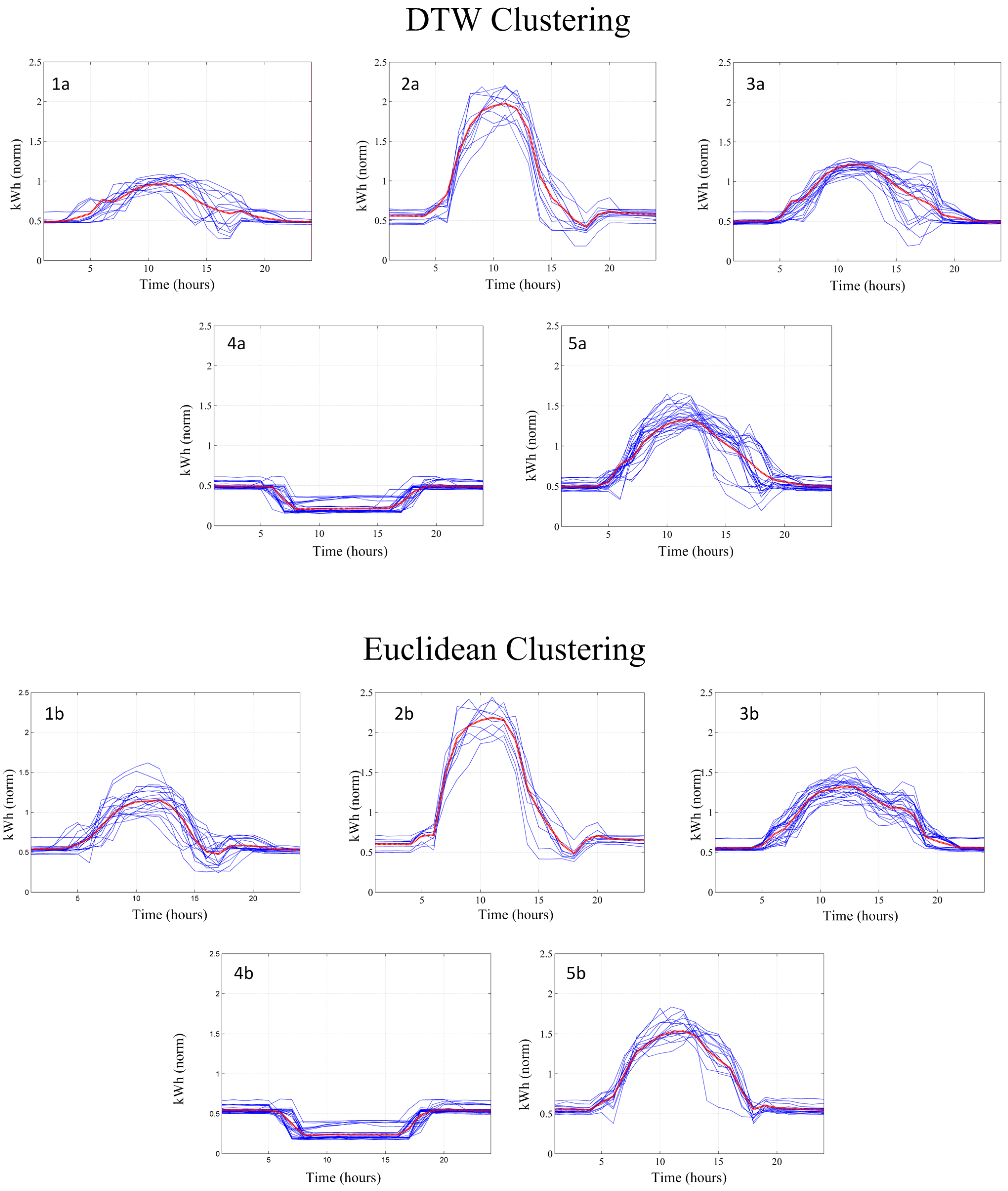
DTW distance deserves a special mention as it has been the most successful in the evaluation test and in finding the best clusters. We can expect that in related prediction applications it performs as good as the Euclidean distance and sometimes even better. If both similarity measures are compared based on the conducted test, the reasons for the different performances can be inferred (Figure 7 shows an example of discovered patterns and embraced input clusters for both clustering solutions, using DTW and Euclidean similarity measures).

On one hand, using DTW distance for clustering also entails a deformation of the input space in order to better capture the representative nuclei. It ensures that the clusters’ gravity centers move toward areas where high-correlated samples (or parts of the samples) are better represented, sacrificing capabilities to represent or embrace samples that do not show such high-correlation or coincidence. But, compared with Mahalanobis or Correlation distances, the induced deformation is more respectful with the overall shape or structure that forms the input samples all together. Figure 7 is a good example to check Euclidean clustering, not only compared with DTW, but with all the considered measures that somehow estimate correlation (where DTW has proved to be the most suitable). At first sight, to visually compare between the two clustering solutions is not easy, both seem to capture the essential patterns with minimum variation. DTW distance favors samples that show parts that really match one another, being more lax if the rest of the curve does not fit such coincidence. This can be seen in Figure 7. Note that, as a general rule, the DTW solution shows more dark zones (curves are closer) as a result of the obsession to find correlated parts. The two equivalent patterns labeled “3a" and “3b" are a good example to assess this phenomenon. Here, in the DTW case, the effort made to fix the high-correlated first part of the profile is significantly spoiled by the less-coincidental last part of the profile. Otherwise, the group found by the Euclidean solution may display a better trade-off, balanced solution.

In short, and according to the test results, the DTW distance usually better defines the important clusters, losing representativeness in the less correlated ones; otherwise, Euclidean metric could result in main cluster representatives that are not so good, but better in order to define the lower-density ones and to summarize the input space as a whole.

Finally, even though a priori computer resources are not a limiting factor in the introduced application case, the time required by the clustering process in every one of the tested configurations is worthy of consideration. Only by changing the similarity measure, the required time by the clustering task shows a different order of magnitude: Euclidean similarity takes hundredths of seconds (0.0Xs); Mahalanobis metric, tenths (0.Xs); Correlation needs seconds (Xs); and DTW distance, tens of seconds (X0s). These values must not be taken as absolute measures, but only to compare clustering performances with one another. Please, note that the processing time depends on the machine used for computation.

Figure 7. Patterns discovered using DTW and Euclidean measures in “Rectorat” building, and embraced samples.

Figure 7. Patterns discovered using DTW and Euclidean measures in “Rectorat” building, and embraced samples.

10. Conclusions

The present paper has introduced and successfully tested clustered-vector balance, a validation measure for comparing clustering solutions based on clustering balance foundations. This technique is not only useful to improve the adjustment and selection of parameters, algorithms and tools for clustering, but also useful to provide information about the reliability of models obtained from clustering, improving context awareness of predictors and controllers.

On the other hand, popular similarity distances—Euclidean, Mahalanobis, Pearson’s correlation distance and DTW—are compared in a time series clustering scenario related to building energy consumption. Although data show strong correlations among vectors and also among features, Euclidean distance is the measure that obtains the best, balanced general solutions. However, DTW distance can be considered as an improved alternative in applications that make the most of a better representation of the high-similar nuclei (or parts of the samples), and where losing capabilities to capture and average the not-so-similar samples is not a critic factor. In short, unlike classic considerations, we hypothesize that only a strong correlation in time series clustering does not justify the use of similarity distances that consider data correlation rather than the Euclidean metric.

Seeking for the implementation of accurate controllers and predictors, part of the current ongoing work consists of checking metrics after outlier removal. Here, an outlier is seen as an element that pertains to a group of non-grouped samples or background vectors. Therefore, annoying elements are temporarily removed in order to get a clearer classification. Later on, outliers are relocated in the solution space, identified as background noise or just definitively removed. The definition of outlier itself is a confusing issue. Dealing with outliers entails additional uncertainties and trade-off decisions and also requires improvements in the validation techniques to evaluate the distinct possible performances.