Performance Analysis of a District Heating System

Abstract

Lowering the exergy content of heat required for heating purposes decreases the primary energy consumption. District heating systems are often an important link between facilities that generate heat with low exergy content and consumers. Exergetic efficiency of heat distribution is an important performance criterion in heat supply to consumers. It can serve as a criterion for optimization, towards a more sustainable distribution-network design and operation. This paper presents a methodology for an exergy-based distribution-network analysis in a district heating system. Criteria for performance evaluations are defined. They can be used to evaluate heat supply to different points in the network, or individual system components. A case study is performed on an existing district heating system. Energetic and exergetic efficiencies of supply lines are analyzed. Exergy destructions and exergy losses are studied. Large differences in efficiency of heat supply to different points in the network are discovered. Over-dimensioned parameters of the distribution network are investigated.

1. Introduction

Exergy of a fossil-fuel stream is very close to its energy value. The exergy of a material stream at temperatures of heated buildings or domestic hot water is typically of the magnitude of 10% of its energy value. Direct usage of boilers to supply heat therefore results in large thermodynamic irreversibility. This irreversibility is in exergy analysis, dependent on the selected boundaries, known as exergy destruction and exergy loss. High values of exergy destruction and loss represent a loss in potential to cause a change. This represents a waste of primary energy resources [1].

Several applications of an exergy analysis to space heating in buildings have been reported in the literature. In Reference [2], it is stated that energy and exergy analyses must be conducted from the primary energy transformation until the building envelope including the envelope. It is shown that the energy concept alone is not adequate in gaining a full understanding of all important aspects of energy utilization processes. The building sector has a high potential for reducing the exergy content of energy demand and supply [3]. For this purpose the exergy concept is relevant for design of buildings as well as heating, ventilation and air-conditioning systems [4,5]. The low exergy approach aims at constituting a sustainable built environment [6]. Low exergy (or LowEx) building systems are studied by many researchers and are seen as a possibility for designing high-performance buildings [3,6,7].

A prerequisite for low-exergy building systems is the supply of low-exergy heat with low irreversibility during generation. This can be achieved by different means. In Reference [8] researchers studied different examples of heat pump systems and compared them to conventional condensation boiler heating systems. The most efficient case in their analyses is a ground source heat pump system which uses 25% less primary energy and exergy compared to a condensation boiler system. In Reference [9] geothermal resources are proposed to be classified as low, medium and high-quality resources based on their exergy value. High-quality resources can be used for the direct generation of electricity. Lower-quality resources are more appropriate for heating applications and their utilization results in lower irreversibility. Solar radiation represents a high-quality energy flow. Researchers in Reference [10] proposed a different boundary when analyzing solar energy systems from an exergy perspective. They stated that thermal energy output of a solar collector field at its corresponding temperature level and electricity output of a PV system should be regarded as “primary energy” sources. In this way inconsistencies from a physical point of view, when regarding direct (e.g., solar thermal, photovoltaic systems or windows in the building envelope) and indirect (e.g., heat pumps, wind turbines, etc.) use of solar radiation, are avoided. This consideration adds solar energy to heat generation systems with low irreversibility.

Cogeneration is a technique for generating multiple energy products simultaneously in a manner of utilizing high-exergy flows for processes where they are needed and the remaining low-exergy flows where they can be used. Thus an important reduction in irreversibility is achieved in comparison with the separate generation of these products. Cogeneration is often related to generation of electricity and heat with low exergy content for heating and industrial purposes. Exergy-based analyses of combined heat and power systems offer clear view and benefits compared with an energy analysis [11].

Low-exergy heat generation is often possible only at a scale which greatly exceeds the local heat demands. In some cases the higher scale of heat generation facilities results in better energetic and exergetic efficiency. In these cases a district heating system (DHS) can be used to connect consumers to the heat generation facility. There the distribution network (DN) of a DHS becomes an important part in the heat supply chain. Areas with low population density or small building complexes are generally not suitable for district heating, as the investment cost per household would be considerable [12]. In addition, heat losses occur on the DN and pumping power is needed to transport the fluid. An exergy-based performance analysis of the DN in a DHS is needed to identify the design and operating parameters that can decrease irreversibility of heat supply to consumers. Several authors have used the exergy concept to analyze DHS [13,14,15,16,17,18]. One study [19] proposed a model which can serve as a basis for differential tariff determination: different price factors were calculated for heat supplied to different consumers based on the exergy losses of heat distribution. Torío et al. [20] presents strategies for improving the performance of waste-heat based DHS. It was concluded that an exergy analysis has a clear added value for characterizing and improving the performance of DHS. Some studies are also dealing with exergoeconomic analyses of DHS. In Reference [21] various studies conducted on geothermal DHS from the energetic, exergetic and exergoeconomic points of view are reviewed.

The DN of a DHS is often spread out in a large area. The hot-water pipes have a variety of diameters and isolative properties. The heat transported through an arbitrary point in the network can vary significantly. The distance from the heat generation facilities to the individual consumers depends on the point in the DN. Accordingly an energetic or exergetic efficiency of the whole DN in a DHS is not informative of the performance of heat supply to individual consumers connected to the network. In order to improve the performance of a DHS from the exergetic or economic point of view, several points in the network have to be considered. We have not found such a model in the literature.

2. Methodology

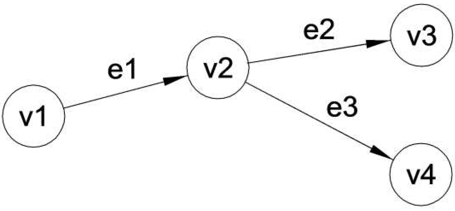
2.1. Network Description

The DN in a DHS is described in this paper using graphs. A graph is a set of points and lines connecting some pairs of the points [22]. The points are called vertices and the lines are called edges. Edges represent connections between points and can be given with individual properties. A connected graph which has no cycles is called a tree. The DN in a DHS without internal loops can be represented by a directed tree. Figure 1 shows a simple directed tree. In the DN this tree structure can be seen as follows. The first vertex in the network is v1. This is the first point which is subject to analysis. The parameters of the supply and return water here determine the thermal inputs into the DN. The edge e1 is a supply line connecting point v2 to v1. From v2 two edges (supply lines) are connecting vertices v3 and v4. Vertices v2 to v4 represent branching and/or consumers or just arbitrary points in the network. To input graphs into a computer, an incidence matrix is used.

Figure 1. Tree structure of a simple DN.

Figure 1. Tree structure of a simple DN.

2.2. Energetic Analysis

A positive effect (PE) of a DN is the heat supplied to the consumers. The resource expended (RE) to do it is the heat supplied to the DN (${\dot{Q}}_{sup}$) and the energy required for the pumps ($\dot{W}$). The DN heat losses are denoted by ${\dot{Q}}_L$. We can write an energy balance equation for the whole system:

$${\dot{E}}_{RE}={\dot{E}}_{PE}+{\dot{Q}}_L={\dot{Q}}_{sup}+\dot{W}$$

(1)

In analogy the PE and the RE can be defined for each individual supply line (edge in Figure 1). Resource expended can also be considered as resources needed to supply heat to an individual point in the network. e.g., heat which has to be supplied to the vertex v1 and energy for the pumps to supply the product to v3. Accordingly, the definition of RE and PE depends on the chosen control volume. Because conversion of mechanical energy to heat occurs in the DN, in addition to heat transportation, the term energetic efficiency is used as an energy-based criterion for performance evaluation. It is defined by Equation (2):

$$\eta =\frac{{\dot{E}}_{PE}}{{\dot{E}}_{RE}}$$

(2)

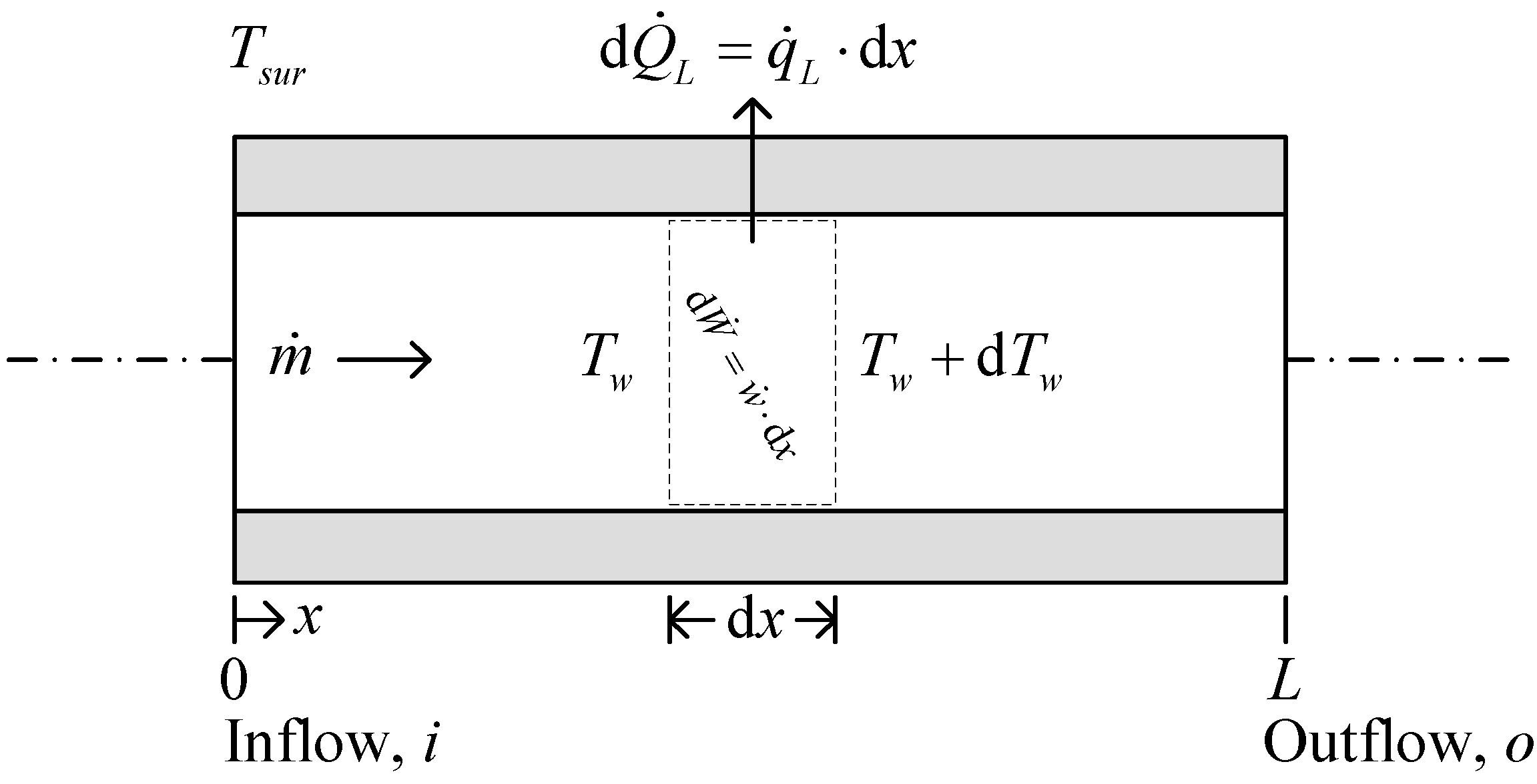
2.2.1. Differential Energy Equation for a Control Volume in Pipe

A flow of liquid in district heating pipes is closed. Its temperature T_w(x) along the length of the pipeline can be determined by an energy equation. A flow in supply or return pipe is displayed in Figure 2. The mass-flow rate is constant. The pressure drop is dependent on the wall shear stress between the water and pipe surface. The overall pressure drop for the pipe system consists of the pressure loss due to viscous effects in the straight pipes termed the major loss and the pressure drop in various other components, termed the minor loss [23].

Figure 2. Control volume for the internal flow in a pipe.

Figure 2. Control volume for the internal flow in a pipe.

In a DN of a DHS the static pressure is maintained at a constant value. Pumping power is needed to cover the pressure losses. Pressure losses are a drop in static pressure over the length of a pipe. Pumps are located at several locations in the network and increase the static pressure. However, the location of the pumps has little influence when analyzing the energy performance of a DN with given flow parameters. Consequently we model the network, for a more generally applicable analysis, as if it would have a large number of pumps, so large, that their effect on the static pressure could be neglected. In this way the whole network (or a part of the network which is physically separated) is considered to have the same static pressure over the length of the pipes. We assume that a specific pumping power [Equation (3)] is being supplied for transporting the liquid through the pipe. In the DN pipes, turbulent flow occurs and a friction factor for the straight pipes is calculated by the Colebrook correlation [24]. In Equation (3) a 20% increment of friction factor is considered to cover the minor losses, as in [18]. The efficiency of the pump is not considered here. We would like to calculate the amount of energy that is required for the transport of liquid but not the power supplied to the pumps. A specific heat flux is defined by Equation (4):

$$\dot{w}=\frac{\left(1.2f\right)\dot{m}{v}^2}{2d}$$

(3)

$${\dot{q}}_L=Uo\left(T_w-T_{sur}\right)$$

(4)

An energy balance for the control volume in Figure 2 is described with Equation (5). It is a first order differential equation and can be solved by reorganization, substitution and integration. In Equation (6) a solution, reorganized for calculation of liquid temperature on the length of the pipe is shown:

$$\dot{m}{c}_p\left[T_w-\left(T_w+\text{d}{T}_w\right)\right]=\text{d}{\dot{Q}}_L-\text{d}\dot{W}={\dot{q}}_L\text{d}x-\dot{w}\text{d}x$$

(5)

$$T_o(x)=\frac{\text{exp}\left(-\frac{Uox}{\dot{m}{c}_p}\right)·\left(Uo\left(T_i-T_{sur}\right)-\dot{w}\right)+\dot{w}}{Uo}+T_{sur}$$

(6)

2.2.2. Pumping Power and Heat Losses

The pumping power needed to supply the hot water to the consumers is calculated using Equation (7). To calculate the pipe heat losses, Equation (8) is used:

$$\dot{W}=\dot{w}{\displaystyle \underset{0}{\overset{L}{\int }}\text{d}x}=\frac{\left(1.2f\right)\dot{m}{v}^2}{2d}·L$$

(7)

$${\dot{Q}}_L=\dot{m}{c}_p\left(T_i-T_o\right)+\dot{W}$$

(8)

2.3. Exergetic Analysis

The system boundaries and definitions used in this paper are in accordance with a widely used and accepted theory in exergoeconomics [1,25].

2.3.1. Reference State

In a reference state the system is in equilibrium with the environment. A DHS is a closed system. Consumers and heat generation facilities are usually physically separated from the DN. In an interaction with the environment only thermal energy is being transferred. Thus a restricted reference state exists, where temperature of the water is equal to the temperature of the environment. The pressure and chemical potential remain unchanged. The available exergy in a water flow in the DN is therefore defined by calculating the thermal part of the physical exergy [26]:

$$e_w^T={\left[\left(h_w-h_{w,T_0}\right)-T_0\left(s_w-s_{w,T_0}\right)\right]}_{p=const}$$

(9)

2.3.2. Boundaries on Supply and Return Lines

The exergy balance for a component as well as for the overall system can be written in the form exergy of fuel/exergy of product [1]. Exergy of product is the desired result, expressed in exergy terms, achieved by the system (component). Exergy of fuel is the exergetic resource expended to generate the product exergy. The exergy of fuel and product for a supply line in Figure 3 is defined with Equations (10) and (11):

$${\dot{E}}_F={\dot{E}}_{sup,v1}-{\dot{E}}_{ret,v1}+{\dot{W}}_{sup}+{\dot{W}}_{ret}$$

(10)

$${\dot{E}}_P={\dot{E}}_{sup,v2}-{\dot{E}}_{ret,v2}$$

(11)

Figure 3. Supply line with heat transfer to the surroundings.

Figure 3. Supply line with heat transfer to the surroundings.

The selection of boundaries is an important issue for exergy analysis. The choice of boundary determines whether the effect of heat transfer to the environment is charged as exergy destruction or exergy loss as explained in the following. In Figure 3 a supply line (edge) is defined as a control volume. Heat losses of the supply pipe are denoted as Q_L,sup and heat losses of the return pipe Q_L,ret. Two different boundaries are defined:

• Boundary I includes just the supply and return pipeline, or
• Boundary II is located outside the system where the temperature corresponds to the ambient temperature, considered here as the temperature of the reference environment T₀.

With boundary II, heat transfer occurs at the temperature T₀. There is no associated exergy transfer: ${\dot{E}}_Q=0$. Accordingly, the value of the exergy loss is: ${\dot{E}}_L=0$. The exergy destruction term accounts for exergy destruction owing to friction and the irreversibility of heat transfer to the environment [Equation (12)]. With Boundaries I the rate of exergy loss ${\dot{E}}_L$ equals the rate of exergy transfer associated with heat transfer, and is given by Equation (13):

$${\dot{E}}_D^{\text{Boundary II}}={\dot{E}}_F-{\dot{E}}_P$$

(12)

$${\dot{E}}_L^{\text{Boundary I}}={\displaystyle \underset{v1}{\overset{v2}{\int }}\left(1-\frac{T_0}{T_w}\right)}·{\dot{q}}_L·\text{d}x$$

(13)

With different boundary considerations, the exergies of fuel and product remain the same. The relation between exergy destruction and exergy loss with different boundaries is described by Equation (14):

$${\dot{E}}_D^{\text{Boundary II}}={\dot{E}}_D^{\text{Boundary I}}+{\dot{E}}_L^{\text{Boundary I}}$$

(14)

With the definitions of the exergies of product and fuel, the exergetic efficiency for the selected control volume is calculated by Equation (15). The ratio of the exergy destruction rate to the exergy loss rate is given by Equation (16). This ratio is defined to study the relation between exergy destruction and exergy loss in cases of optimal and non-optimal design and operation of the DN:

$$\epsilon =\frac{{\dot{E}}_P}{{\dot{E}}_F}$$

(15)

$$y_{DL}=\frac{{\dot{E}}_D^{\text{Boundary I}}}{{\dot{E}}_L^{\text{Boundary I}}}$$

(16)

2.4. Consideration of Return Pipes

Supply pipes distribute water from one vertex to others in a tree structure. The direction of water flow in the return pipes is the opposite. Let us consider that consumers at v3 and v4 in Figure 1 are returning water with the same temperature. When edges e2 and e3 are not identical, the temperature of both return flows is not the same in v2. Mixing takes place in this case and also when the consumers are returning water with different temperatures. This affects the exergy fuel through heat losses of the return pipeline and the return water temperature in v1. Accordingly the return temperature of one consumer affects the efficiency of supplying heat to other consumers. In a DHS there are usually consumers with higher and lower return temperatures. Supplying heat to consumers with higher return temperatures reduces the DN efficiency and supplying heat to consumers with low return temperatures increases it. Accordingly it is appropriate to separate the efficiencies of heat supply to different consumers as much as possible. We can achieve this by individually considering the return of each consumer. To do it first the return in v4 (Figure 1) defines the temperature in v2 and v1. For the return in vertices v3 and v2 the calculations are then repeated. The mass flow rates in the return pipes are on all edges of the same value as in the supply pipes. With this consideration we can calculate different efficiencies for consumers with different return temperatures. Because of lower heat losses of the return than the supply pipeline, the difference to actual conditions is small.

3. Case Study

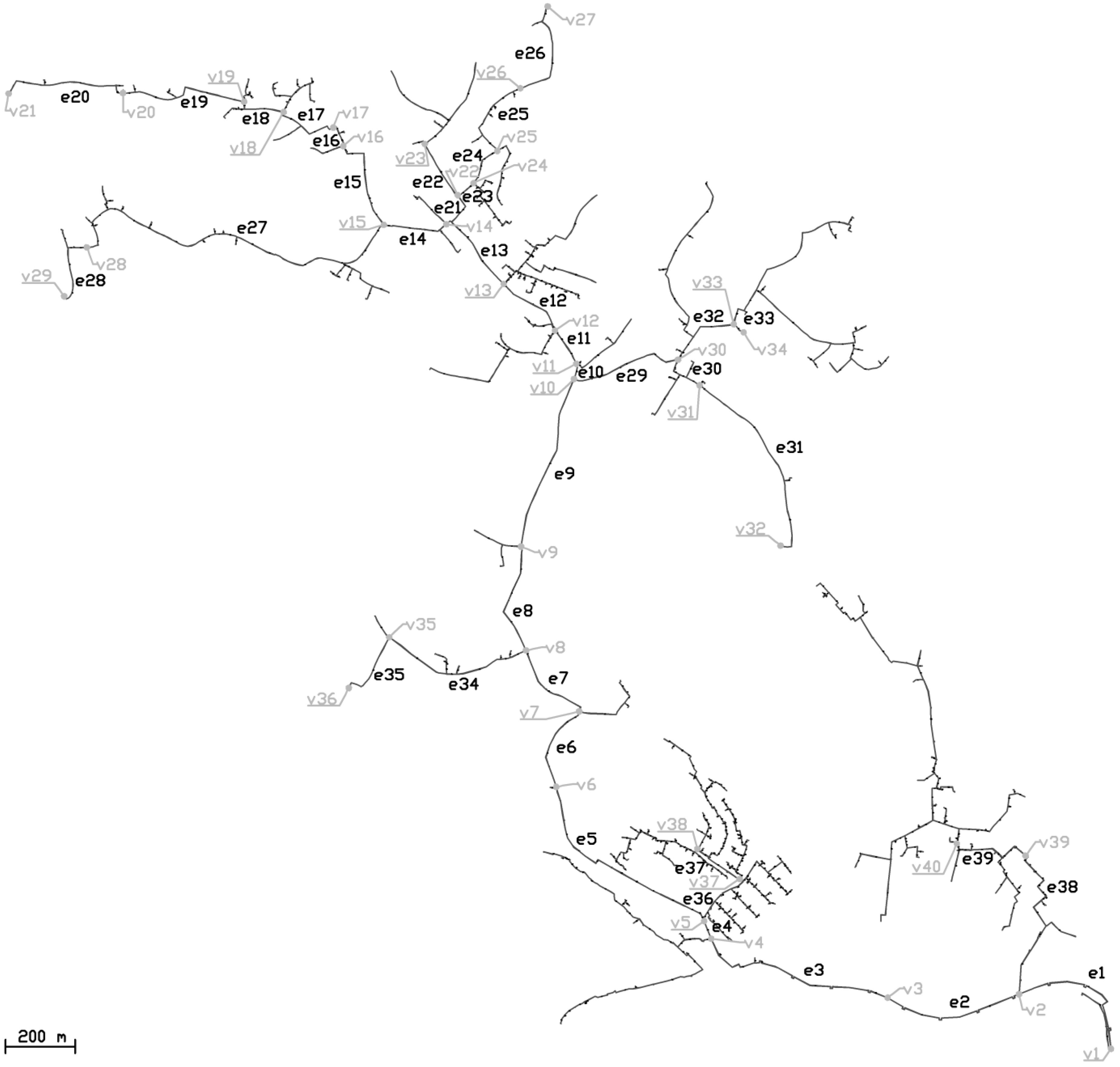
3.1. District Heating of Šaleška Valley

In Slovenia 9% of total heat demand in residential, services and other sectors is supplied by district heating. In Šaleška Valley, which is positioned in the northern part of the country, Slovenia’s second largest DHS is in operation. The heat is produced by a coal-fired cogeneration plant. Coal is extracted locally in one of the largest and most modern underground thick layer mines in Europe [27]. The electrical power of the cogeneration plant is 779 MW. The maximal heating power supplied to the DN is 192 MW. Cooling towers are used for the heat, which has to be transferred to the surroundings in the electricity production process and is not supplied to the DN. A part of the DN is analyzed in this paper. It covers approximately 15% of the total DN. The analyzed part is presented as a tree structure in Figure 4. To this part of the network, heat is supplied through vertex v1. Following vertices were introduced where a change in pipe diameter, water mass-flow rate, pipe insulation properties or branching of the network occurs.

Figure 4. Tree structure of the considered DN in Šaleška valley.

Figure 4. Tree structure of the considered DN in Šaleška valley.

The physical parameters, defined for pipes include the pipe diameter, length, overall heat transfer coefficient and pressure in pipes. A surrounding temperature for each pipe is defined. Stationary conditions on a winter day are considered in our case study. Heat flow supplied to vertices is shown in Table 1. The considered data was acquired while determining the energetic efficiency of the DN [28] and are summarized in Table 2. The supply lines e1–e4 are above ground and all the remaining lines are underground. That is why there are differences in their surrounding temperatures. The pressure in supply pipes is 16 bar and in return pipes 15 bar. The temperature of the environment is 0.2 °C. The same parameters from Table 2 are considered for the supply and return pipes. The water velocities are within the interval 0.37 to 0.44 m/s.

Table 1. Heat flow, supplied to vertices.

Vertex	v2	v5	v8	v10	v14	v15	v21	v25	v27	v28
${\dot{E}}_{PE}$, MW	8.50	3.77	2.34	2.28	1.25	1.24	0.08	0.23	0.08	0.20
Vertex	v29	v30	v32	v34	v35	v36	v38	v39	v40	–
${\dot{E}}_{PE}$, MW	0.07	0.37	0.11	0.09	0.20	0.05	0.38	0.59	0.37	–

Table 1. Heat flow, supplied to vertices.

Vertex	v2	v5	v8	v10	v14	v15	v21	v25	v27	v28
${\dot{E}}_{PE}$, MW	8.50	3.77	2.34	2.28	1.25	1.24	0.08	0.23	0.08	0.20
Vertex	v29	v30	v32	v34	v35	v36	v38	v39	v40	–
${\dot{E}}_{PE}$, MW	0.07	0.37	0.11	0.09	0.20	0.05	0.38	0.59	0.37	–

Table 2. Physical parameters of edges in DN in Šaleška valley (stationary conditions on a winter day).

Edge	d, mm	L, m	U, W/m2K	Tsur, °C	Edge	d, mm	L, m	U, W/m2K	Tsur, °C	Edge	d, mm	L, m	U, W/m2K	Tsur, °C
e1	350	455	0.64	0.2	e14	150	168	1.02	8.2	e27	65	1068	1.53	8.2
e2	350	445	0.64	0.2	e15	125	292	1.12	8.2	e28	40	220	1.94	8.2
e3	250	626	0.78	0.2	e16	125	72	1.12	8.2	e29	80	323	1.38	8.2
e4	250	55	0.78	0.2	e17	80	184	1.38	8.2	e30	60	120	1.59	8.2
e5	200	630	0.88	8.2	e18	76	134	1.42	8.2	e31	48	600	1.77	8.2
e6	200	259	0.88	8.2	e19	60	377	1.59	8.2	e32	76	211	1.42	8.2
e7	200	253	0.88	8.2	e20	42	368	1.89	8.2	e33	42	37	1.89	8.2
e8	200	321	0.88	8.2	e21	150	96	1.02	8.2	e34	60	438	1.59	8.2
e9	200	510	0.88	8.2	e22	114	181	1.17	8.2	e35	32	212	2.18	8.2
e10	150	46	1.02	8.2	e23	125	58	1.12	8.2	e36	250	191	0.78	8.2
e11	150	115	1.02	8.2	e24	65	122	1.53	8.2	e37	80	159	1.38	8.2
e12	150	216	1.02	8.2	e25	60	255	1.59	8.2	e38	100	515	1.24	8.2
e13	150	267	1.02	8.2	e26	42	309	1.89	8.2	e39	80	243	1.38	8.2

Table 2. Physical parameters of edges in DN in Šaleška valley (stationary conditions on a winter day).

Edge	d, mm	L, m	U, W/m2K	Tsur, °C	Edge	d, mm	L, m	U, W/m2K	Tsur, °C	Edge	d, mm	L, m	U, W/m2K	Tsur, °C
e1	350	455	0.64	0.2	e14	150	168	1.02	8.2	e27	65	1068	1.53	8.2
e2	350	445	0.64	0.2	e15	125	292	1.12	8.2	e28	40	220	1.94	8.2
e3	250	626	0.78	0.2	e16	125	72	1.12	8.2	e29	80	323	1.38	8.2
e4	250	55	0.78	0.2	e17	80	184	1.38	8.2	e30	60	120	1.59	8.2
e5	200	630	0.88	8.2	e18	76	134	1.42	8.2	e31	48	600	1.77	8.2
e6	200	259	0.88	8.2	e19	60	377	1.59	8.2	e32	76	211	1.42	8.2
e7	200	253	0.88	8.2	e20	42	368	1.89	8.2	e33	42	37	1.89	8.2
e8	200	321	0.88	8.2	e21	150	96	1.02	8.2	e34	60	438	1.59	8.2
e9	200	510	0.88	8.2	e22	114	181	1.17	8.2	e35	32	212	2.18	8.2
e10	150	46	1.02	8.2	e23	125	58	1.12	8.2	e36	250	191	0.78	8.2
e11	150	115	1.02	8.2	e24	65	122	1.53	8.2	e37	80	159	1.38	8.2
e12	150	216	1.02	8.2	e25	60	255	1.59	8.2	e38	100	515	1.24	8.2
e13	150	267	1.02	8.2	e26	42	309	1.89	8.2	e39	80	243	1.38	8.2

The supply water temperature in vertex v1 is 126.5 °C. The temperature of the return in each vertex is 75 °C. An exergy analysis of heat exchangers is relatively simple on a level needed for DN. In addition the main goal of the case study in this paper is to present the tree structure exergy analysis with different boundaries and definitions of exergies of fuel and product. Therefore a part of the DN is selected which does not contain any heat exchangers.

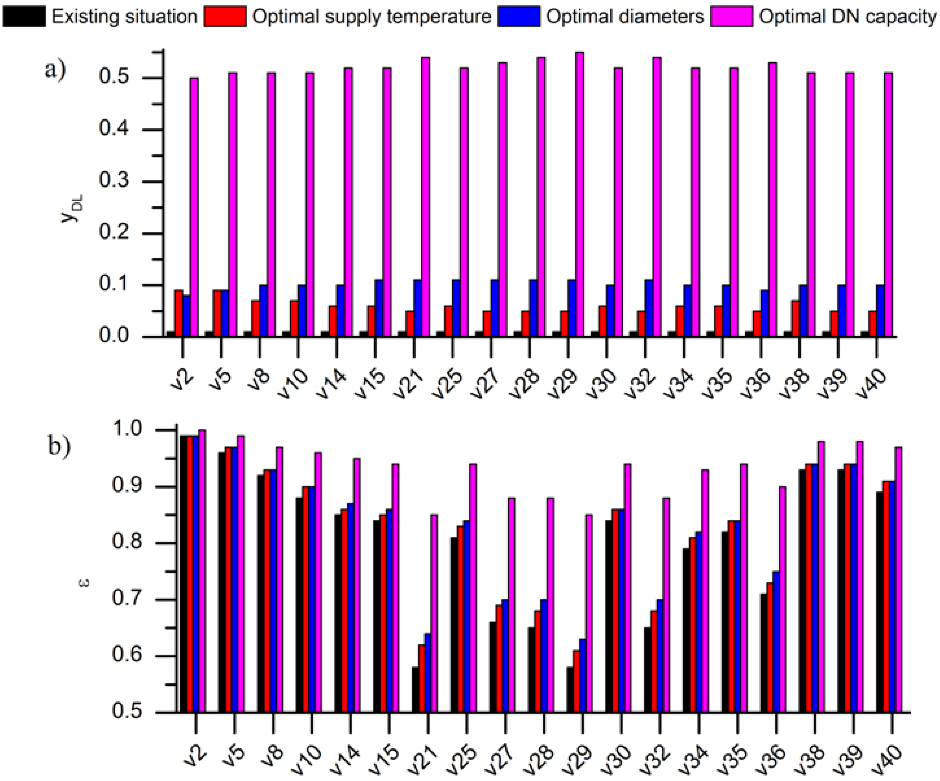
3.2. Results and Discussion

In Table 3 results of the performance analysis on a part of the DN in Šaleška valley are presented. Representative vertices from Figure 4 are selected. Three different possibilities for the DN performance improvement are studied to discover the over-dimensioned parameters in the existing stationary situation. Table 3 is divided into four sections: existing stationary situation, optimal supply temperature, optimal pipe diameters and optimal network capacity. The optimal values were determined by iterative optimization. In this procedure individual parameters are determined at which the given amount of heat is transported with the highest exergy efficiency to the selected object. To transport sufficient heat flows, the mass flow-rates are also changed. With the optimal supply temperatures, the object is selected where almost no investment is needed. With the optimal pipe diameters, the object is complete reconstruction of the network and operation in existing temperature regime. In the case of the optimal network capacity a non-realistic increment of transported heat is studied to discover the maximal possible DN efficiency in the existing temperature regime. Results show that the variations among indicators that determine the efficiency of heat supply to different points in the network are high in all studied cases.

In the existing stationary situation the least efficient operation is the heat supply to vertex v29. The supply water temperature there is 15.4 °C lower than in v1. A low energy and exergetic efficiency is calculated there. The exergy destruction to loss ratios have very low values for all vertices. This implies that measures which would increase the exergy destructions and decrease the exergy losses might improve the efficiency of heat supply.

In the optimal supply temperature columns in Table 3 a preposition is made that the return temperature cannot be reduced due to consumer requirements. The supply temperature to vertex v1 is lowered and the mass flow rates on individual edges are increased to meet the former heat demands (Table 1). This procedure is iteratively continued until the exergetic efficiency of heat supply is increased. At this point the maximum exergetic efficiency for the given constraints is achieved. This occurs at a supply temperature of 100.5 °C.

In the optimal diameters column in Table 3, the supply and return pipe diameters are shown at which heat is transported to vertices with the highest exergetic efficiency. Supply and return temperatures remain unchanged. Optimal diameters are searched in series, first for heat supply from v1 to v2, then from v2 to v3 and so on until v40. The overall heat transfer coefficients from Table 2 are adjusted to smaller diameters. It is found that higher energetic and exergetic efficiencies would be achieved with smaller supply and return pipe sizes. Due to lower temperatures in return pipes, their thermodynamically optimal size is larger than the supply pipes.

The optimal distribution network capacity is investigated by increasing the water mass flow rates in pipes and thus increasing the amount of heat distributed through the network. This is not based on any real possibilities for increased heat demands of consumers in the system. The purpose is to find the effect of the increased heat demands on the improved performance of the DN operation in the same temperature regime. Optimal capacity is searched in series, from v1 to v40. In this procedure the mass-flow rate on edges is iteratively increased until the exergetic efficiency is increased. Because the exergetic efficiency is a concave function, a maximum is discovered. While doing this, all other parameters from Section 3.1 are not changed. The maximal occurring water velocities are 2 m/s.

Table 3. Results from the energetic and exergetic analyses.

Vertex	Existing stationary situation (Tsup,v1 = 126.5 °C)				Optimal supply temperature (Tsup,v1 = 100.5 °C)				Optimal pipe diameters (Tsup,v1 = 126.5 °C)						Optimal DN capacity (Tsup,v1 = 126.5 °C)
	TW, °C	η	ε	yDL	TW, °C	η	ε	yDL	dsup, mm	dret, mm	TW, °C	η	ε	yDL	${\dot{E}}_{PE}$	TW, °C	η	ε	yDL
v2	126.3	0.99	0.99	0.01	100.4	0.99	0.99	0.09	216	259	126.3	0.99	0.99	0.08	33.3	126.4	1.00	1.00	0.50
v5	125.4	0.97	0.96	0.01	100.1	0.97	0.97	0.09	139	167	125.7	0.97	0.97	0.09	17.7	126.3	0.99	0.99	0.51
v8	123.9	0.92	0.92	0.01	99.5	0.93	0.93	0.07	110	134	124.6	0.94	0.93	0.10	11.2	126.0	0.98	0.97	0.51
v10	122.8	0.89	0.88	0.01	99.1	0.90	0.90	0.07	109	134	123.8	0.91	0.90	0.10	11.2	125.8	0.97	0.96	0.51
v14	121.5	0.85	0.85	0.01	98.5	0.87	0.86	0.06	80	99	122.9	0.88	0.87	0.10	6.4	125.5	0.97	0.95	0.52
v15	121.1	0.84	0.84	0.01	98.4	0.86	0.85	0.06	80	99	122.6	0.88	0.86	0.11	6.4	125.5	0.96	0.94	0.52
v21	111.2	0.60	0.58	0.01	94.2	0.63	0.62	0.05	21	27	115.1	0.67	0.64	0.11	0.5	123.7	0.90	0.85	0.54
v25	120.3	0.82	0.81	0.01	98.1	0.84	0.83	0.06	34	42	122.0	0.86	0.84	0.11	1.3	125.3	0.96	0.94	0.52
v27	114.4	0.67	0.66	0.01	95.6	0.70	0.69	0.05	21	27	117.6	0.73	0.70	0.11	0.5	124.3	0.92	0.88	0.53
v28	114.0	0.66	0.65	0.01	95.4	0.69	0.68	0.05	33	42	117.3	0.73	0.70	0.11	1.3	124.2	0.92	0.88	0.54
v29	111.1	0.60	0.58	0.01	94.1	0.63	0.61	0.05	19	26	115.0	0.67	0.63	0.11	0.5	123.7	0.90	0.85	0.55
v30	121.2	0.85	0.84	0.01	98.4	0.86	0.86	0.06	43	53	122.6	0.88	0.86	0.10	1.9	125.5	0.96	0.94	0.52
v32	114.0	0.66	0.65	0.01	95.4	0.69	0.68	0.05	24	31	117.2	0.72	0.70	0.11	0.7	124.3	0.92	0.88	0.54
v34	119.6	0.80	0.79	0.01	97.8	0.82	0.81	0.06	22	27	121.5	0.84	0.82	0.10	0.5	125.2	0.95	0.93	0.52
v35	120.4	0.83	0.82	0.01	98.1	0.85	0.84	0.06	32	39	122.1	0.86	0.84	0.10	1.1	125.4	0.96	0.94	0.52
v36	116.3	0.72	0.71	0.01	96.4	0.75	0.73	0.05	17	21	118.8	0.77	0.75	0.09	0.3	124.7	0.94	0.90	0.53
v38	124.4	0.94	0.93	0.01	99.7	0.94	0.94	0.07	43	52	124.9	0.95	0.94	0.10	1.9	126.1	0.98	0.98	0.51
v39	124.3	0.93	0.93	0.01	99.7	0.94	0.94	0.05	55	65	124.9	0.95	0.94	0.10	3.0	126.1	0.99	0.98	0.51
v40	123.0	0.90	0.89	0.01	99.2	0.91	0.91	0.05	43	52	124.0	0.92	0.91	0.10	1.9	125.9	0.98	0.97	0.51

Table 3. Results from the energetic and exergetic analyses.

Vertex	Existing stationary situation (Tsup,v1 = 126.5 °C)				Optimal supply temperature (Tsup,v1 = 100.5 °C)				Optimal pipe diameters (Tsup,v1 = 126.5 °C)						Optimal DN capacity (Tsup,v1 = 126.5 °C)
	TW, °C	η	ε	yDL	TW, °C	η	ε	yDL	dsup, mm	dret, mm	TW, °C	η	ε	yDL	${\dot{E}}_{PE}$	TW, °C	η	ε	yDL
v2	126.3	0.99	0.99	0.01	100.4	0.99	0.99	0.09	216	259	126.3	0.99	0.99	0.08	33.3	126.4	1.00	1.00	0.50
v5	125.4	0.97	0.96	0.01	100.1	0.97	0.97	0.09	139	167	125.7	0.97	0.97	0.09	17.7	126.3	0.99	0.99	0.51
v8	123.9	0.92	0.92	0.01	99.5	0.93	0.93	0.07	110	134	124.6	0.94	0.93	0.10	11.2	126.0	0.98	0.97	0.51
v10	122.8	0.89	0.88	0.01	99.1	0.90	0.90	0.07	109	134	123.8	0.91	0.90	0.10	11.2	125.8	0.97	0.96	0.51
v14	121.5	0.85	0.85	0.01	98.5	0.87	0.86	0.06	80	99	122.9	0.88	0.87	0.10	6.4	125.5	0.97	0.95	0.52
v15	121.1	0.84	0.84	0.01	98.4	0.86	0.85	0.06	80	99	122.6	0.88	0.86	0.11	6.4	125.5	0.96	0.94	0.52
v21	111.2	0.60	0.58	0.01	94.2	0.63	0.62	0.05	21	27	115.1	0.67	0.64	0.11	0.5	123.7	0.90	0.85	0.54
v25	120.3	0.82	0.81	0.01	98.1	0.84	0.83	0.06	34	42	122.0	0.86	0.84	0.11	1.3	125.3	0.96	0.94	0.52
v27	114.4	0.67	0.66	0.01	95.6	0.70	0.69	0.05	21	27	117.6	0.73	0.70	0.11	0.5	124.3	0.92	0.88	0.53
v28	114.0	0.66	0.65	0.01	95.4	0.69	0.68	0.05	33	42	117.3	0.73	0.70	0.11	1.3	124.2	0.92	0.88	0.54
v29	111.1	0.60	0.58	0.01	94.1	0.63	0.61	0.05	19	26	115.0	0.67	0.63	0.11	0.5	123.7	0.90	0.85	0.55
v30	121.2	0.85	0.84	0.01	98.4	0.86	0.86	0.06	43	53	122.6	0.88	0.86	0.10	1.9	125.5	0.96	0.94	0.52
v32	114.0	0.66	0.65	0.01	95.4	0.69	0.68	0.05	24	31	117.2	0.72	0.70	0.11	0.7	124.3	0.92	0.88	0.54
v34	119.6	0.80	0.79	0.01	97.8	0.82	0.81	0.06	22	27	121.5	0.84	0.82	0.10	0.5	125.2	0.95	0.93	0.52
v35	120.4	0.83	0.82	0.01	98.1	0.85	0.84	0.06	32	39	122.1	0.86	0.84	0.10	1.1	125.4	0.96	0.94	0.52
v36	116.3	0.72	0.71	0.01	96.4	0.75	0.73	0.05	17	21	118.8	0.77	0.75	0.09	0.3	124.7	0.94	0.90	0.53
v38	124.4	0.94	0.93	0.01	99.7	0.94	0.94	0.07	43	52	124.9	0.95	0.94	0.10	1.9	126.1	0.98	0.98	0.51
v39	124.3	0.93	0.93	0.01	99.7	0.94	0.94	0.05	55	65	124.9	0.95	0.94	0.10	3.0	126.1	0.99	0.98	0.51
v40	123.0	0.90	0.89	0.01	99.2	0.91	0.91	0.05	43	52	124.0	0.92	0.91	0.10	1.9	125.9	0.98	0.97	0.51

The comparison of exergetic efficiency and exergy destruction to loss ratio in the considered cases is shown in Figure 5. The exergy destruction to loss ratio is higher, compared to the existing situation, in all three cases of improved performance. The exergy destruction to loss ratio is, in cases of optimal supply temperatures and optimal diameters, in the range of 0.05 to 0.11. It is higher in the case of optimal capacity: 0.5 to 0.55. In the optimal capacity case, the maximal exergetic efficiency is achieved for transporting arbitrary amounts of heat in a given design of the network and the existing temperature regime. It is the highest possible performance of the network. In the other two optimization cases, the maximum exergetic efficiency is searched for a given amount of required heat. Accordingly we can separate two different approaches to DN optimization. In cases where a DN already exists, the highest exergetic efficiency for the stationary conditions are achieved, when the exergy destruction to loss ratio is low (around 0.1 in our case). If the heat demand is high, after the network is built, the exergetic efficiency will improve. In the case analyzed here (Table 3) it is improving until an exergy destruction to exergy loss ratio of approximately 0.53 is reached. E.g., in the optimal DN capacity case the peak exergetic efficiency of the network is achieved. However, if the network would be designed for these amounts of transported heat, even higher exergetic efficiencies would be achieved by selecting larger pipes.

In Figure 5b it can be seen that the highest exergetic efficiency of the considered cases is achieved at optimal DN capacity. This shows the importance of having a sufficient heat demand in an urban area for efficient heat distribution.

Figure 5. Results: (a) Exergy destruction to loss ratio; (b) Exergetic efficiency.

Figure 5. Results: (a) Exergy destruction to loss ratio; (b) Exergetic efficiency.

4. Conclusions

A methodology for an exergy-based analysis of a DN in a DHS is presented. The main difference with other published papers on this subject are in the definition of energetic and exergetic efficiencies for a single point in the DN and in the exergy balance in the form of product exergy/fuel exergy. Possibilities for efficiency improvements of different parts of the network are discovered in this way. To investigate the utilization of primary energy sources, the energy conversion chain efficiency must be considered, before a DN is recommended.

Separation of the exergy destruction and exergy losses points out guidelines for exergetic efficiency improvements. The choice of boundaries is important when doing this separation. A low-exergy destruction to exergy loss ratio suggests that increasing the pumping power and decreasing the heat losses will improve the exergetic efficiency of the DN. The optimal exergy destruction to loss ratio depends on the studied case, optimization constraints and boundary conditions. Thus it needs to be investigated in each individual case. However it is lower in the DN design stage than at the maximal possible exergetic efficiency of an existing DN.

Analysis of a part of the DN in Šaleška Valley has demonstrated the large differences in energetic and exergetic efficiencies of heat supply to different points in the network. The exergy destruction to loss ratio in the existing stationary situation is 0.01. Accordingly we can conclude that the network is operating below its optimal capacity.

The exergetic efficiency can be used as a criterion for optimization to decrease the irreversibility of heat distribution. Three different exergetic efficiency optimization procedures are executed to find out the scale of over-dimensioned design parameters in an existing stationary situation. Higher exergetic efficiencies of heat supply to different points in the network are achieved by reducing the supply temperature, reducing the pipe sizes or increasing the heat transported through the network. The optimal supply pipe diameters are smaller than the return diameters.

References

1. Bejan, A.; Tsatsaronis, G.; Moran, M.J. Thermal Design and Optimization; Wiley-Interscience: New York, NY, USA, 1996. [Google Scholar]
2. Yildiz, A.; Güngör, A. Energy and exergy analyses of space heating in buildings. Appl. Energy 2009, 86, 1939–1948. [Google Scholar] [CrossRef]
3. Hepbasli, A. Low exergy (LowEx) heating and cooling systems for sustainable buildings and societies. Renew. Sustain. Energy Rev. 2012, 16, 73–104. [Google Scholar] [CrossRef]
4. Sakulpipatsin, P.; Itard, L.C. M.; van der Kooi, H.J.; Boelman, E.C.; Luscuere, P.G. An exergy application for analysis of buildings and HVAC systems. Energy Build. 2010, 42, 90–99. [Google Scholar] [CrossRef]
5. Balta, M.T.; Dincer, I.; Hepbasli, A. Performance and sustainability assessment of energy options for building HVAC applications. Energy Build. 2010, 42, 1320–1328. [Google Scholar] [CrossRef]
6. Balta, M.T.; Kalinci, Y.; Hepbasli, A. Evaluating a low exergy heating system from the power plant through the heat pump to the building envelope. Energy Build. 2008, 40, 1799–1804. [Google Scholar] [CrossRef]
7. Meggers, F.; Ritter, V.; Goffin, P.; Baetschmann, M.; Leibundgut, H. Low exergy building systems implementation. Energy 2011, 41, 48–55. [Google Scholar] [CrossRef]
8. Lohani, S.; Schmidt, D. Comparison of energy and exergy analysis of fossil plant, ground and air source heat pump building heating system. Renew. Energy 2010, 35, 1275–1282. [Google Scholar] [CrossRef]
9. Lee, K.C. Classification of geothermal resources by exergy. Geothermics 2001, 30, 431–442. [Google Scholar] [CrossRef]
10. Torío, H.; Schmidt, D. Framework for analysis of solar energy systems in the built environment from an exergy perspective. Renew. Energy 2010, 35, 2689–2697. [Google Scholar] [CrossRef]
11. Feidt, M.; Costea, M. Energy and exergy analysis and optimization of combined heat and power systems. comparison of various systems. Energies 2012, 5, 3701–3722. [Google Scholar] [CrossRef]
12. Reverberi, A.; Borghi, A.D.; Dovì, V. Optimal design of cogeneration systems in industrial plants combined with district heating/cooling and underground thermal energy storage. Energies 2011, 4, 2151–2165. [Google Scholar] [CrossRef]
13. Çomaklı, K.; Yüksel, B.; Çomaklı, Ö. Evaluation of energy and exergy losses in district heating network. Appl. Therm. Eng. 2004, 24, 1009–1017. [Google Scholar] [CrossRef]
14. Ozgener, L.; Hepbasli, A.; Dincer, I. Energy and exergy analysis of geothermal district heating systems: An application. Build. Environ. 2005, 40, 1309–1322. [Google Scholar] [CrossRef]
15. Ozgener, L.; Hepbasli, A.; Dincer, I. Exergy analysis of two geothermal district heating systems for building applications. Energy Convers. Manag. 2007, 48, 1185–1192. [Google Scholar] [CrossRef]
16. Keçebaş, A.; Kayfeci, M.; Gedik, E. Performance investigation of the Afyon geothermal district heating system for building applications: Exergy analysis. Appl. Therm. Eng. 2011, 31, 1229–1237. [Google Scholar] [CrossRef]
17. Yüksel, B.; Aslan, A.; Akyol, T. Investigation of seasonal variations in the energy and exergy performance of the Gonen geothermal district heating system. Appl. Therm. Eng. 2012, 36, 39–50. [Google Scholar] [CrossRef]
18. Li, H.; Svendsen, S. Energy and exergy analysis of low temperature district heating network. Energy 2012, 45, 237–246. [Google Scholar] [CrossRef]
19. Poredoš, A.; Kitanovski, A. Exergy loss as a basis for the price of thermal energy. Energy Convers. Manag. 2002, 43, 2163–2173. [Google Scholar] [CrossRef]
20. Torío, H.; Schmidt, D. Development of system concepts for improving the performance of a waste heat district heating network with exergy analysis. Energy Build. 2010, 42, 1601–1609. [Google Scholar] [CrossRef]
21. Hepbasli, A. A review on energetic, exergetic and exergoeconomic aspects of geothermal district heating systems (GDHSs). Energy Convers. Manag. 2010, 51, 2041–2061. [Google Scholar] [CrossRef]
22. Voloshin, V.I. Introduction to Graph Theory; Nova Science Publishers: New York, NY, USA, 2009. [Google Scholar]
23. Munson, B.R.; Young, D.F.; Okiishi, T.H. Dimensional analysis of pipe flow. In Fundamentals of Fluid Mechanics; Fowley, D., Ed.; Wiley: New York, NY, USA, 1998; Volume 3, p. 410. [Google Scholar]
24. Incropera, F.P.; Bergman, T.L.; Lavine, A.S.; de Witt, D.P. Fundamentals of Heat and Mass Transfer; Wiley: Hoboken, NJ, USA, 2011. [Google Scholar]
25. Tsatsaronis, G. Definitions and nomenclature in exergy analysis and exergoeconomics. Energy 2007, 32, 249–253. [Google Scholar] [CrossRef]
26. Morosuk, T.; Tsatsaronis, G. Graphical models for splitting physical exergy. In Shaping Our Future Energy Systems, Proceedings of the 18th International Conference on Efficiency, Cost, Optimization, Simulation, and Environmental Impact of Energy Systems (ECOS), Trondheim, Norway, 20–22 June 2005; pp. 377–384.
27. Medved, M.; Ristovic, I.; Roser, J.; Vulic, M. An overview of two years of continuous energy optimization at the velenje coal mine. Energies 2012, 5, 2017–2029. [Google Scholar] [CrossRef]
28. Ljubenko, A.; Poredoš, A. Energy efficiency of a district heating system and its possible improvements. In Proceedings of 24th International Conference on Efficiency, Cost, Optimization, Simulation and Environmental Impact of Energy Systems, Novi Sad, Serbia, 4–7 July 2011; pp. 2935–2944.