Load Forecast Model Switching Scheme for Improved Robustnessto Changes in Building Energy Consumption Patterns

Abstract

This paper presents a new, accurate load forecasting technique robust to fluctuations due to unusual load behavioral changes in buildings, i.e., the potential for small commercial buildings with heterogeneous stores. The proposed scheme is featured with two functional components: data classification by daily characteristics and automatic forecast model switching. The scheme extracts daily characteristics of the input load data and arranges the load data into weekday and weekend data. Forecasting is conducted based on a selected model among ARMAX (autoregressive moving average with exogenous variable) models with the processed input data. Kalman filtering is applied to estimate model parameters. The model-switching scheme monitors the accumulated error and substitutes a backup load model for the currently working model, when the accumulated error exceeds a threshold value, to reduce the increased bias error due to the change in the consumption pattern. This switching reinforces the limited performance of parameter estimation given a fixed structure and, thus, forecasting capability. The study results demonstrate that the proposed scheme is reasonably accurate and even robust to changes in the electricity use patterns. It should help improve the performance for building control systems for energy efficiency.

1. Introduction

Buildings in every shape and size are envisioned to be a huge potential for the efficiency improvement of the power grid, especially because residential and commercial buildings are responsible for about 30- to 40-percent of primary energy consumption worldwide. A rich body of literature for developing high performance energy management systems (EMS) for buildings can be found to achieve significant energy savings [1,2,3]. Among the enabling technologies, load forecasting, in particular, short-term hourly load forecasting [4,5], should be the front-end application of the EMS, because it helps to better understand energy behavior and provides the baseline estimate of future real savings, especially under dynamic pricing. It helps analyze the load shape and variability and determine proper controls or demand response under a grid emergency, as well. The central aim of this paper is thus to develop an accurate and robust scheme for predicting the hourly power use of a building.

Several load forecasting techniques have been studied [6,7,8]. These studies can be categorized into three types: regression techniques [9,10], artificial neural network (ANN)-related methods [11,12,13] and time series approaches [14,15,16]. In regression techniques, linear representations are applied as the main forecasting function, where mathematical relationships among electrical load demand, weather and exogenous variables are intended. This technique has a test-feasibility and short handling of non-stationary temporal cases as an advantage and disadvantage. The ANN uses historical load and weather data to identify the load model and, therefore, has good approximation capabilities for a wide range of nonlinear models. However, the ANN often converges slowly in training mode and needs to manually determine the network structure and parameters.

In time series techniques, load demands are treated as time series signals. This technique predicts load demand using time series analysis. Among these approaches, stochastic time series techniques have the advantage of finding models with a minimum mean square forecasting error. However, the gradient search-based technique used by the basic stochastic time series (STS) approach is prone to finding local optimal points that build an insufficient forecasting model, because the forecasting error function of this approach possesses multiple minimum points. In summary, this approach is sufficient, but involves computational risk caused by numerical instability.

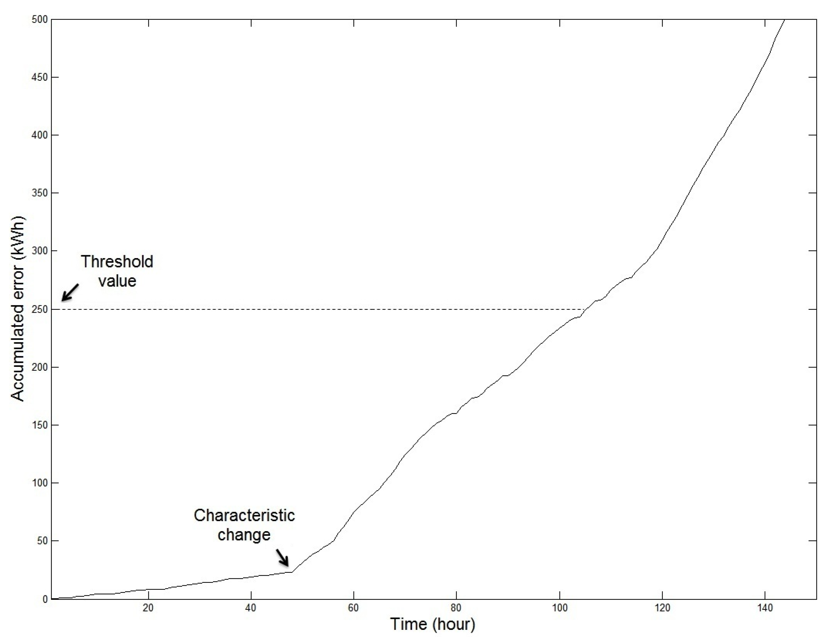
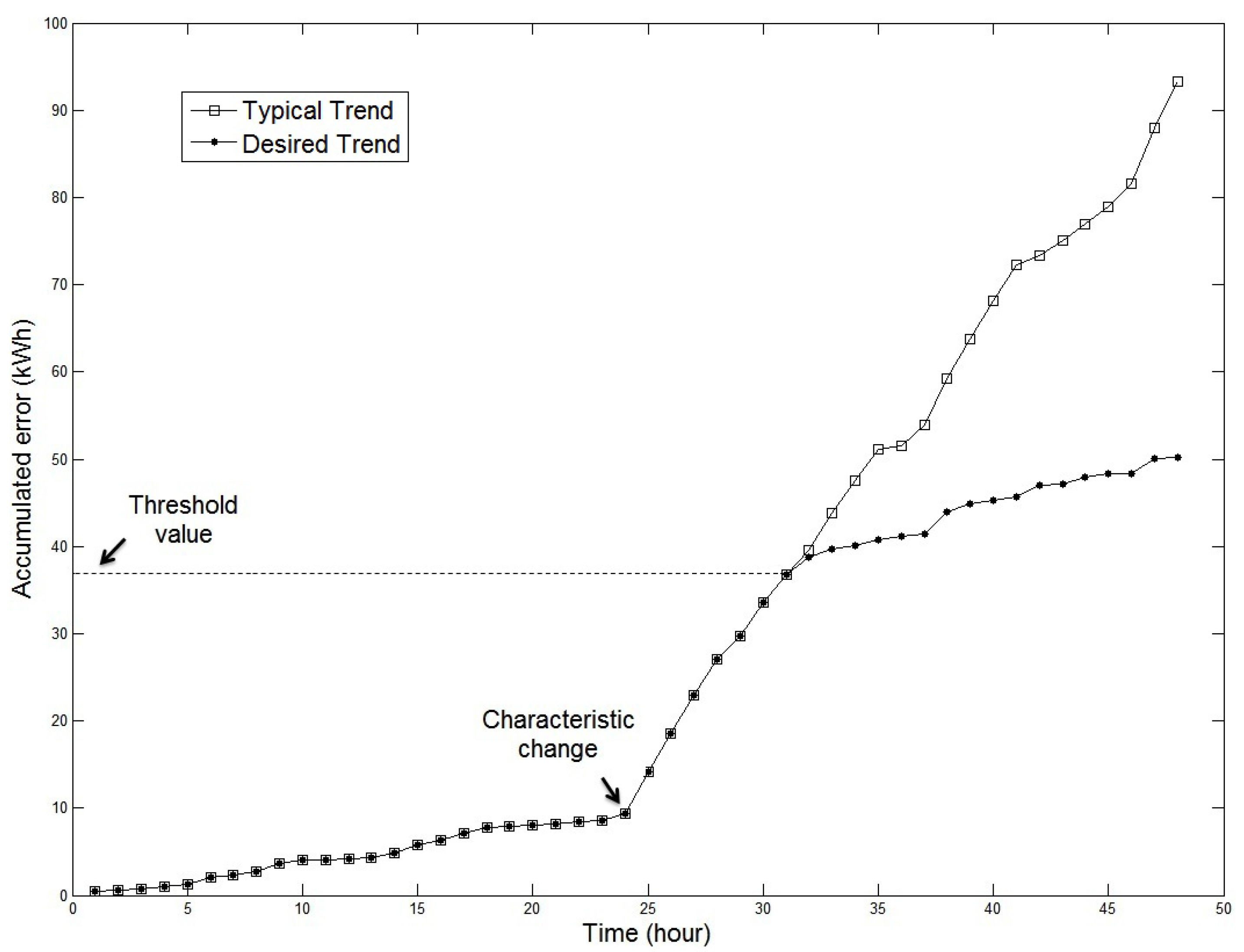
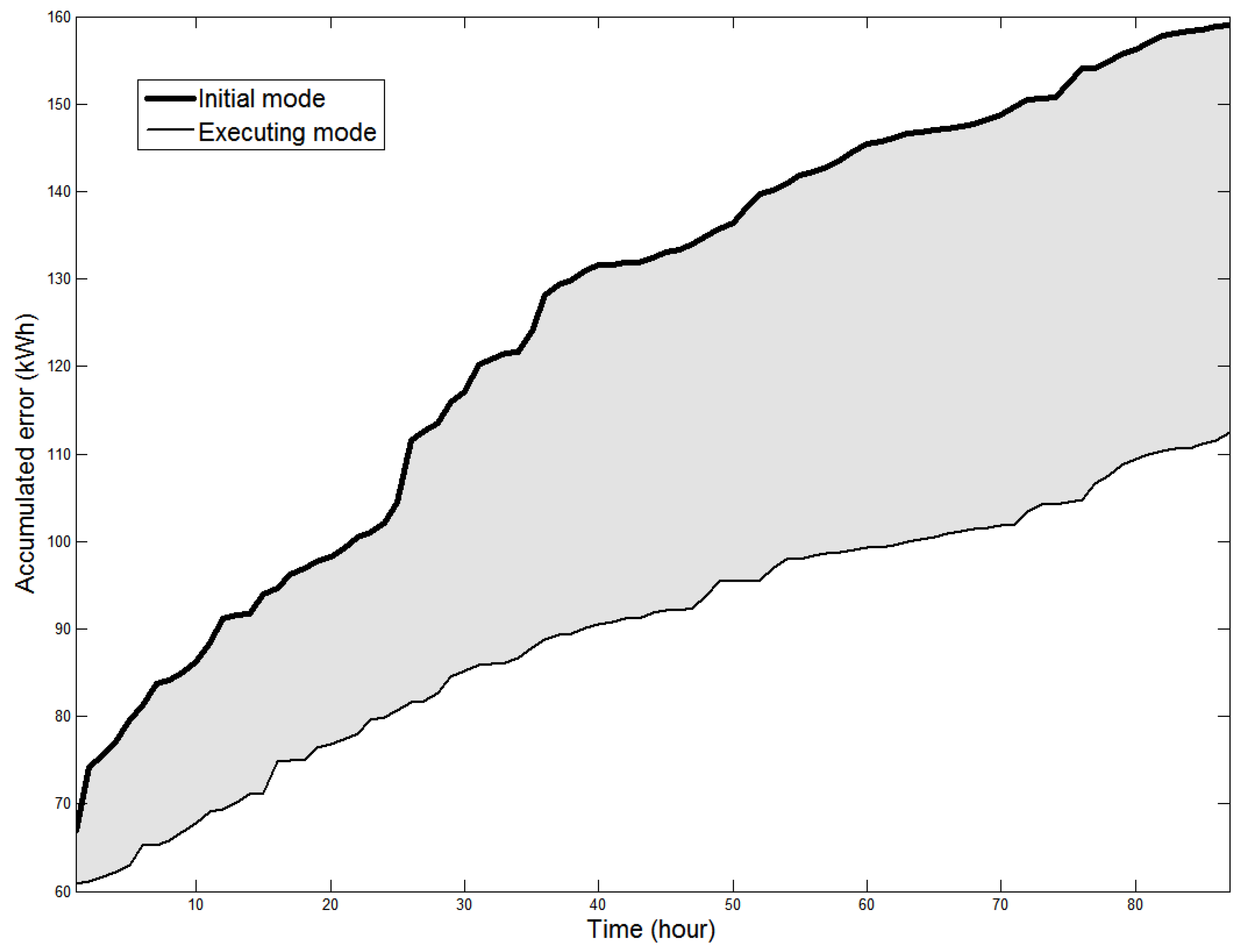
In the case of buildings, the increase of an accumulated error from load characteristic change, caused by consumption patterns and business and working hour changes, can occur. The Figure 1 shows that accumulated errors of the fixed model and our proposed model in load forecasting are increased dramatically when the load characteristic is changed. Figure 1 illustrates a case where the forecasting scheme using a fixed model fails to perform best, and thus, the accumulated error increases dramatically when the load characteristics are changed. It also includes a desired performance obtained through proposed model switching, as detailed in Section 3. Motivated by the observation that many of the previous forecasting methods using a fixed model do not perform well, as the above dynamic change may occur, we propose an accurate load forecasting technique that combines proven forecasting models with different model structures in order to improve the limited performance of existing techniques. In this research, the autoregressive moving average with exogenous variable (ARMAX) model with temperature as the exogenous variable is selected to represent the load behavior [13,17]. Our scheme has two core components: data pattern classification according to weekday and weekend characteristics and model switching in response to the significant change in the accumulated error. The improved robustness and resulting forecasting accuracy should help advance smart grid technologies, including energy management, security analysis, economic dispatch and power scheduling, by forecasting more accurate energy usage.

Figure 1. Trends of increasing accumulated error.

Figure 1. Trends of increasing accumulated error.

The remainder of this paper is organized as follows. Section 2 describes the ARMAX model and Kalman filtering as the forecast model and a tool for estimating parameters of the model. In Section 3, we propose the scheme for improving the accuracy and robustness by changing the model structure and reducing the accumulated error. Section 4 provides numerical study results using MATLAB simulations. Section 5 presents concluding remarks.

2. Background

The load pattern possesses nonlinear and dynamic characteristics, seasonal and diurnal variations and different weather conditions. The ARMAX model selection technique has been extensively studied, because it can describe the relationship between load and extra variables, including weather. In the ARMAX model, the load is denoted as a linear function that has an inaccessible white-noise input and an accessible exogenous input series. The characteristics of the load model are identified based on the variables in the function. The remaining problem becomes finding the proper values of variables in the model, namely parameter estimation.

By adequately constructing the load model and estimating parameters in the function, we can forecast the future load. Thus, an ARMAX-based load model and Kalman filtering for parameter estimation are introduced below as the processes of load forecasting.

2.1. ARMAX-Based Load Model

In this paper, the ARMAX model is used to define the relationship between load and temperature that is regarded as the exogenous variable influencing the load demand, because load demand in a building is susceptible to weather and the number of people in the building. The notation of the ARMAX model for this paper is represented as follows:

$$A\left(q\right)L\left(t\right)=B\left(q\right)u\left(t\right)+C\left(q\right)e\left(t\right)$$

(1)

where $L\left(t\right)$, $u\left(t\right)$ and $e\left(t\right)$ are the load, the exogenous variable and the white noise at time t, respectively; $A\left(q\right)$, $B\left(q\right)$ and $C\left(q\right)$ are the autoregressive (AR) part, the exogenous input part and the moving average (MA) part. Each part has a back-shift operator, q and an order parameter and can be represented as follows:

$$A\left(q\right)=1+a_1{q}^{-1}+\cdots +a_n{q}^{-n},B\left(q\right)=b_1+b_2{q}^{-1}+\cdots +b_m{q}^{-m+1},C\left(q\right)=1+c_1{q}^{-1}+\cdots +c_r{q}^{-r}$$

(2)

where $a_1$, ⋯, $a_n$, $b_1$, ⋯, $b_m$ and $c_1$, ⋯, $c_r$ are parameters of the autoregressive part, the exogenous input part and the moving average part; and n, m and r are the AR order, input order and MA order.

In determining the order number of each part, the sample autocorrelation function (ACF), the sample partial autocorrelation function (PACF) and the cross-correlation function (CCF) are employed [18]. In general, it is challenging to select appropriate model orders, and it is therefore essential to use a technique derived from experience.

In this paper, we modify the ARMAX model for our research. First, we divide the back-shift operator into day and time back-shift operators. Because we concentrate on forecasting energy consumption, and since time and date are important factors in load forecasting, we use the day and the 24 h factor as follows:

$$q^{-n}=>d^{-j}{t}^{-k}$$

(3)

where d and t are the day and time back-shift operator, respectively; and j and k are their respective order. Each order has the following definition:

$$n=24\ast j+k$$

(4)

where j is a natural number; and k is a number from 0 to 23. For example, $n=55$ means that j is 2 and k is 7. Thus, $q^{-55}=d^{-2}{t}^{-7}$, and it means two days and seven hours ago. Second, we define the load, the exogenous variable and the noise term. For the load term, we use the electrical consumption (kWh) of building in an hour. The exogenous variable is defined as outdoor temperature (${}^{\circ }\mathrm{C}$). The last term (noise) is assumed to be white Gaussian noise.

2.2. Kalman Filter for the Parameter Estimation

This research briefly reviews the recursive discrete Kalman filter used for estimating parameters of the ARMAX model in line with the algorithm development. Details of the Kalman filtering approach to estimating parameters can be found in [19,20].

In order to define Kalman filtering, we have to consider the following discrete state equations:

$$x\left(k\right)=F\left(k\right)x(k-1)+v(k-1)$$

(5)

$$z\left(k\right)=H\left(k\right)x\left(k\right)+n\left(k\right)$$

(6)

where $x\left(k\right)$, $F\left(k\right)$, $z\left(k\right)$, $H\left(k\right)$, $v(k-1)$ and $n\left(k\right)$ are vectors of $n\times 1$ system states, the $n\times n$ dimensions of the state transition matrix, $m\times 1$ measurement vectors, the $m\times n$ output matrix, $n\times 1$ system error and $m\times 1$ measurement error, respectively. The noise vectors, $v(k-1)$ and $n\left(k\right)$, are drawn from white Gaussian noise that has a mean of zero and no time correlation, as shown below.

$$E\left[v\right(k\left)\right]=E\left[n\right(k\left)\right]=0$$

(7)

$$E\left[v\left(i\right)v^T\left(j\right)\right]=E\left[n\left(i\right)n^T\left(j\right)\right]=0fori\ne j$$

(8)

$Q_1$ and $Q_2$, covariance matrices, are defined as follows:

$$Q_1=E\left[v\left(k\right)v^T\left(k\right)\right],Q_2=E\left[n\left(k\right)n^T\left(k\right)\right]$$

(9)

Given the a priori estimate of the state vector, $\widehat{x}\left(0\right)={\widehat{x}}_0$, and its error covariance matrix, $P\left(0\right)=P_0$, we set $k=0$ and then apply the basic Kalman filter algorithm to estimate the next state by recursively computing the following equations:

$$K\left(k\right)=\left[F\left(k\right)P\left(k\right)H^T\left(k\right)\right]{[H\left(k\right)P\left(k\right)H^T\left(k\right)+Q_2]}^{-1}$$

(10)

$$\widehat{x}(k+1)=F\left(k\right)\widehat{x}\left(k\right)+K\left(k\right)[z\left(k\right)-H\left(k\right)\widehat{x}\left(k\right)]$$

(11)

$$P(k+1)=[F\left(k\right)-K\left(k\right)H\left(k\right)]P\left(k\right){[F\left(k\right)-K\left(k\right)H\left(k\right)]}^T+K\left(k\right)Q_2{K}^T\left(k\right)$$

(12)

where $K\left(k\right)$ is the Kalman gain. In this Kalman filter algorithm, it is important to choose an a priori estimate of the state ${\widehat{x}}_0$ and its covariance error $P_0$, because an intelligent choice improves the accuracy and decreases the computational complexity of the algorithm. A few measurement vector samples can be considered as initial values for ${\widehat{x}}_0$ and $P_0$ as follow:

$${\widehat{x}}_0={\left[H^T{Q}_2^{-1}H\right]}^{-1}{H}^T{Q}_2^{-1}{z}_0$$

(13)

$$P_0={\left[H^T{Q}_2^{-1}H\right]}^{-1}$$

(14)

For our model, the discrete state equations in Equations (5) and (6) are defined for our forecasting model as follows:

• The state transition matrix, $F\left(k\right)$, is a constant identity matrix;
• The error covariance matrices, $Q_1$ and $Q_2$, are constant identity matrices;
• The state vector, $x\left(k\right)$, has some parameters based on Equation (2);
• The time-varying output matrix, $H\left(k\right)$, is derived from the load demand and temperature.
• The observation value, $z\left(k\right)$, represents the load at time k. $z\left(k\right)=H\left(k\right)x\left(k\right)$ takes the following form, defined by Equations (1–3):

$$\begin{array}{cc}L\left(t\right)=\hfill & \left[\begin{array}{ccccccc}-a_1& ···& -a_{24\ast j_1+k_1}& b_1& b_2& ···& b_{24\ast j_2+k_2}\end{array}\right]\hfill \\ & \times {\left[\begin{array}{ccccccc}L(t-1)& \cdots & L(t-24\ast j_1+k_1)& u\left(t\right)& u(t-1)& \cdots & u(t-(24\ast j_2+k_2)+1)\end{array}\right]}^T\hfill \\ & +\left[\begin{array}{cccc}1& c_1& \cdots & c_{(}t-24\ast j_3+k_3)\end{array}\right]\times {\left[\begin{array}{cccc}e\left(t\right)& e(t-1)& \cdots & e(t-24\ast j_3+k_3)\end{array}\right]}^T\hfill \end{array}$$

(15)

3. Enhanced Robustness of the Proposed Load Forecasting Scheme

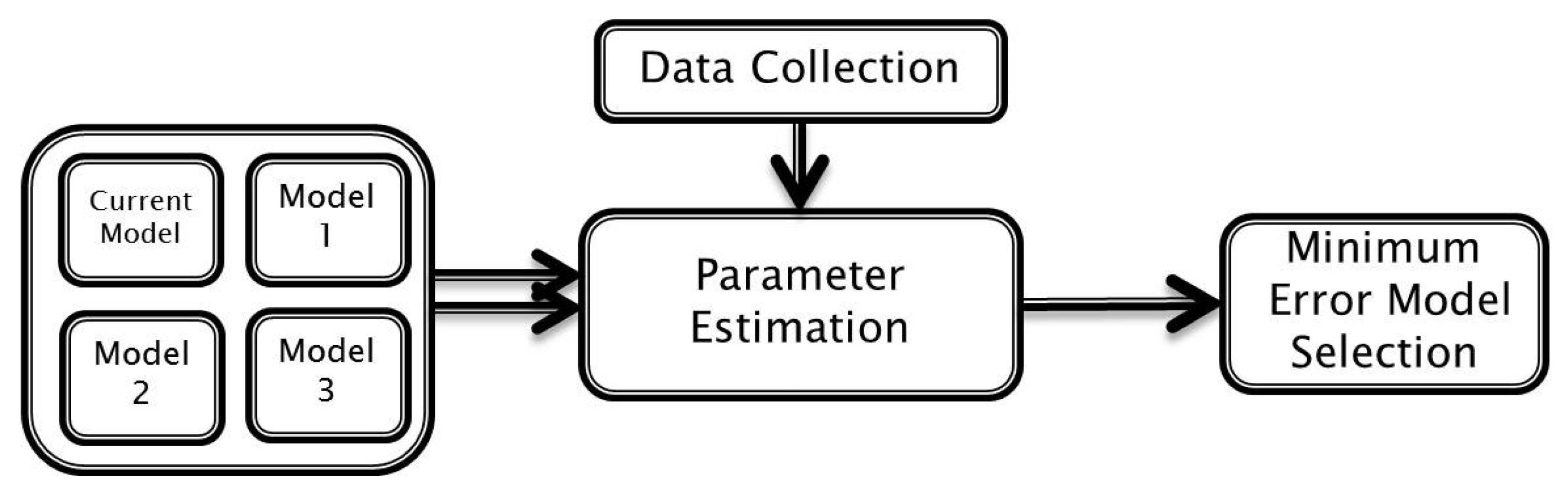
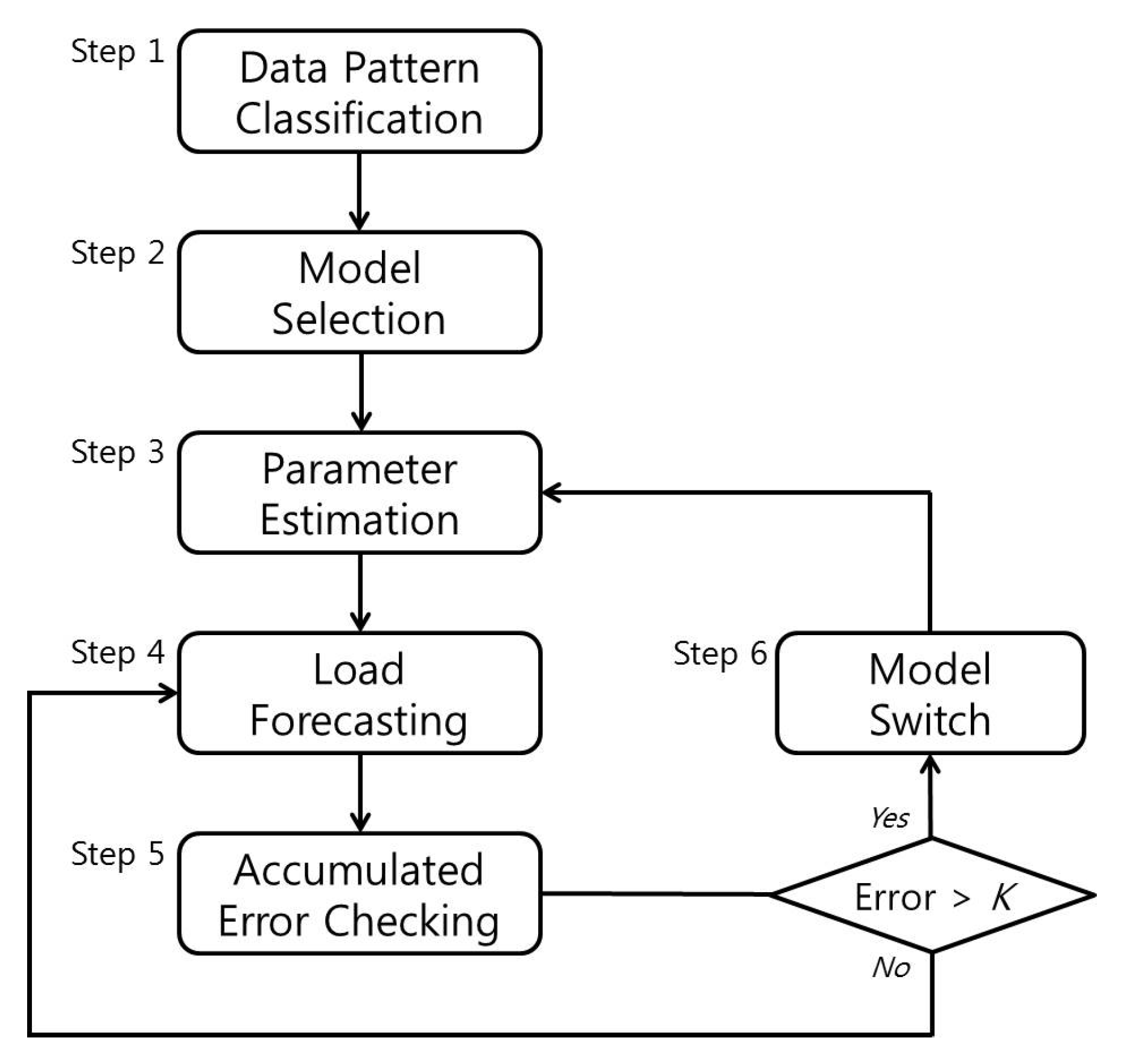
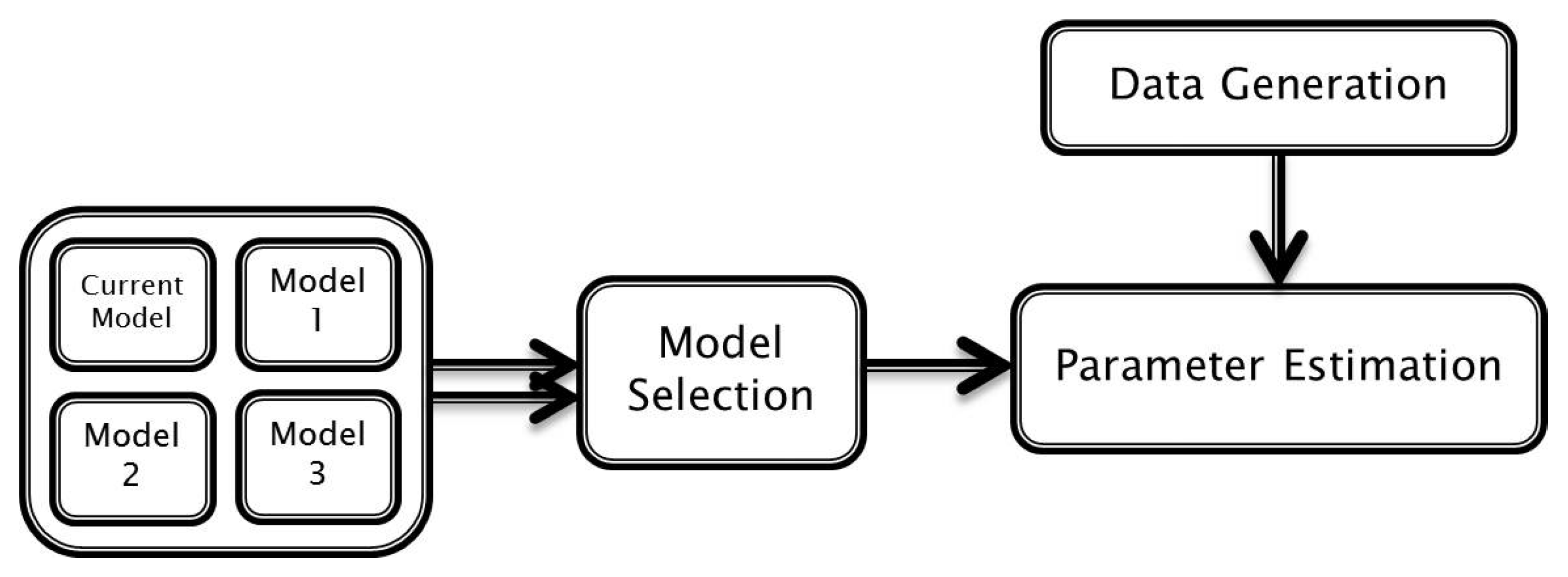
Figure 2 shows the six steps of the proposed robust load forecasting. The first important step is data pattern classification. If the input data are well classified, we can determine a suitable model and reduce forecasting error. The second step, model selection, determines the structure of the forecasting model, model order and load and weather factor using the ARMAX model. The third step is model parameter estimation, during which optimal parameters of the forecasting model are estimated using the Kalman filter and database of past and present load and weather data. The third step leads to a forecast of the load at the next instant of time in the fourth step. The fifth and sixth steps are feedback processes.

Figure 2. Steps for proposed load forecasting scheme.

Figure 2. Steps for proposed load forecasting scheme.

In the fifth process, an accumulated error is obtained by summing up the absolute errors. If it exceeds the reasonable threshold value, K, the sixth step, model-switching scheme (MSS), is executed to replace the model structure. Through this process, we can respond to an increase of accumulated error and reduce total accumulated error. If it does not exceed the threshold value, the fourth step is executed. In this section, we describe data pattern classification for identifying the load model based on day characteristics and a model switching scheme for enhancing forecasting accuracy.

3.1. Data Pattern Classification for Selecting the Load Model

The main purpose of defining a forecasting model is to determine its order and the variables that have effects on the load. As mentioned in Section 2, we use the ARMAX model, which depends on load and temperature. Thus, we collected hourly load data for a building in March 2012, as well as temperature data, in order to reflect day characteristics of input data. Each data point is categorized into two databases, one for the weekday and the other for the weekend.

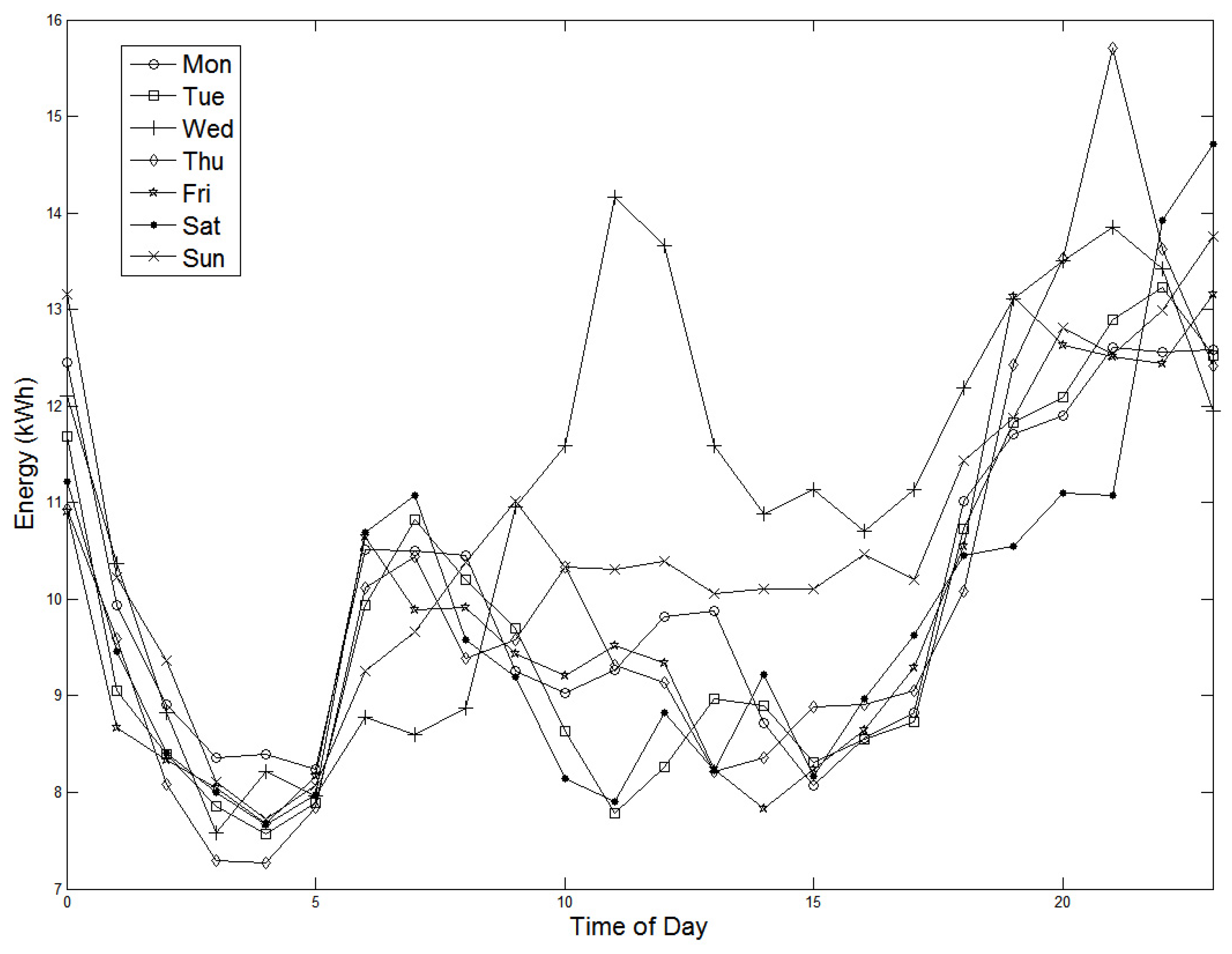
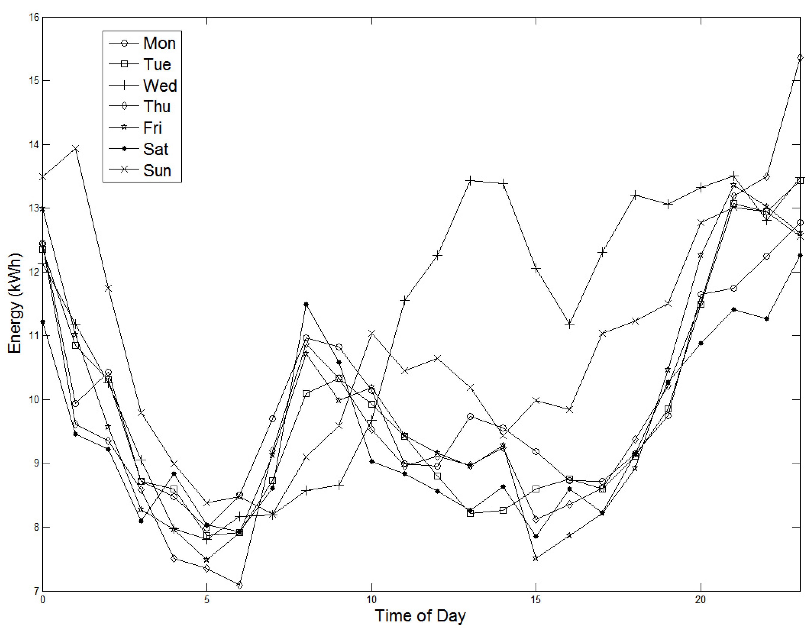
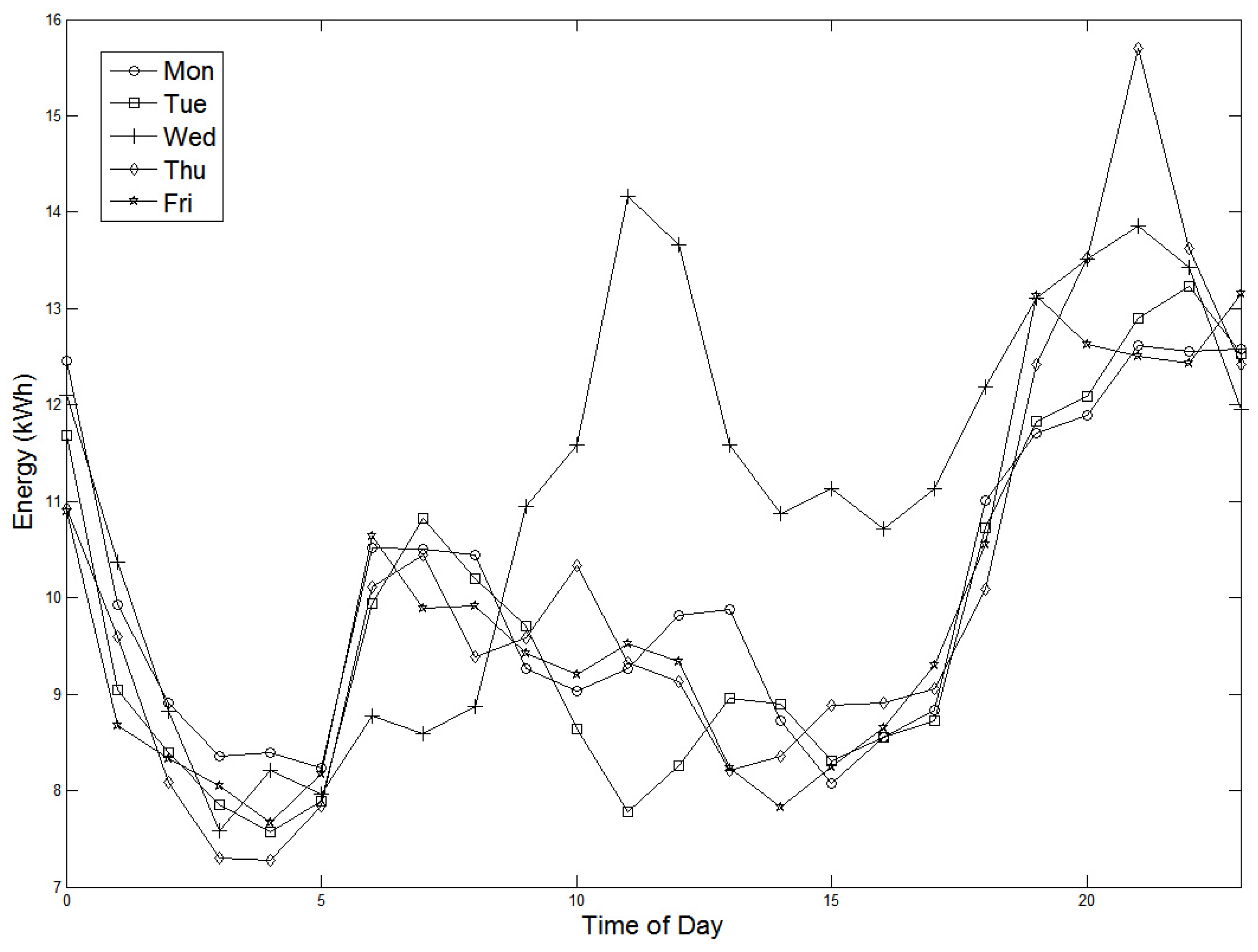
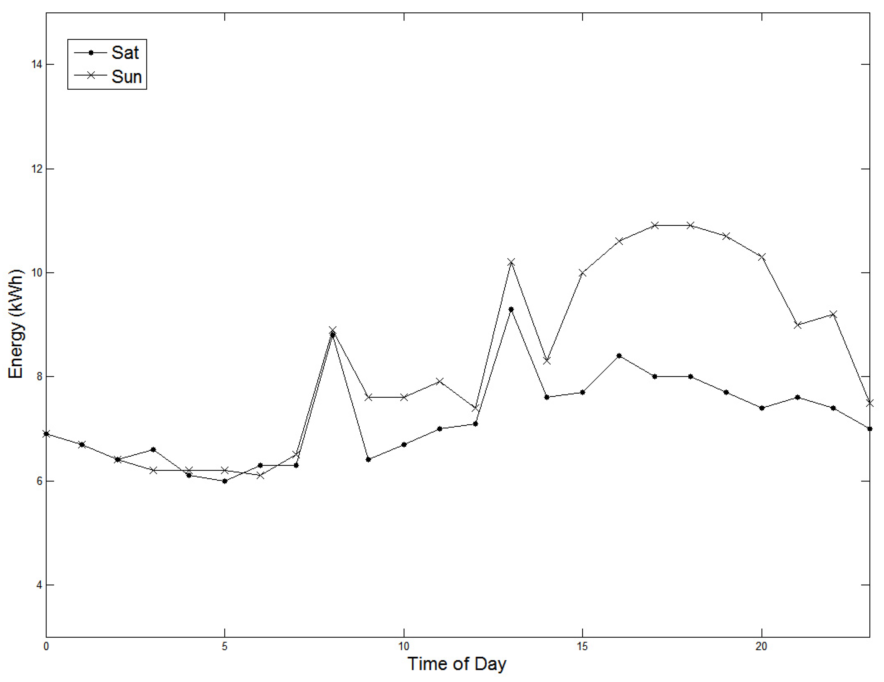
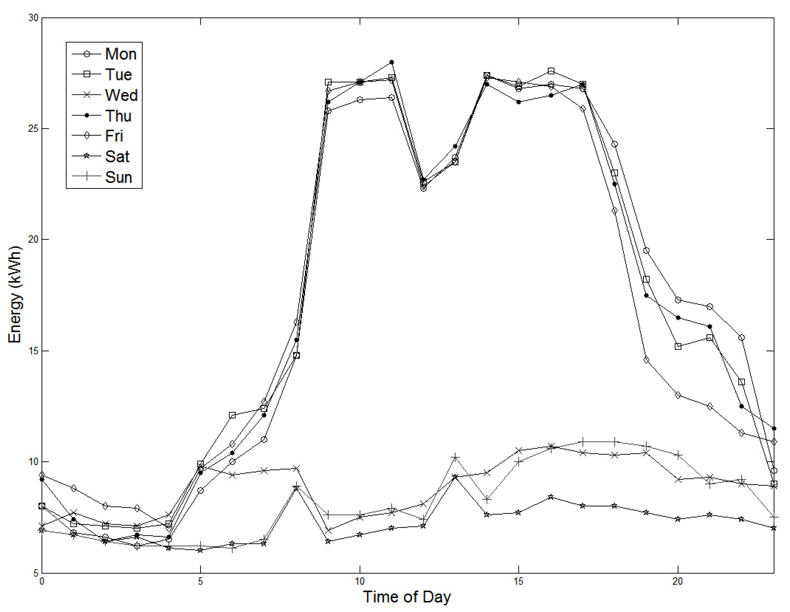
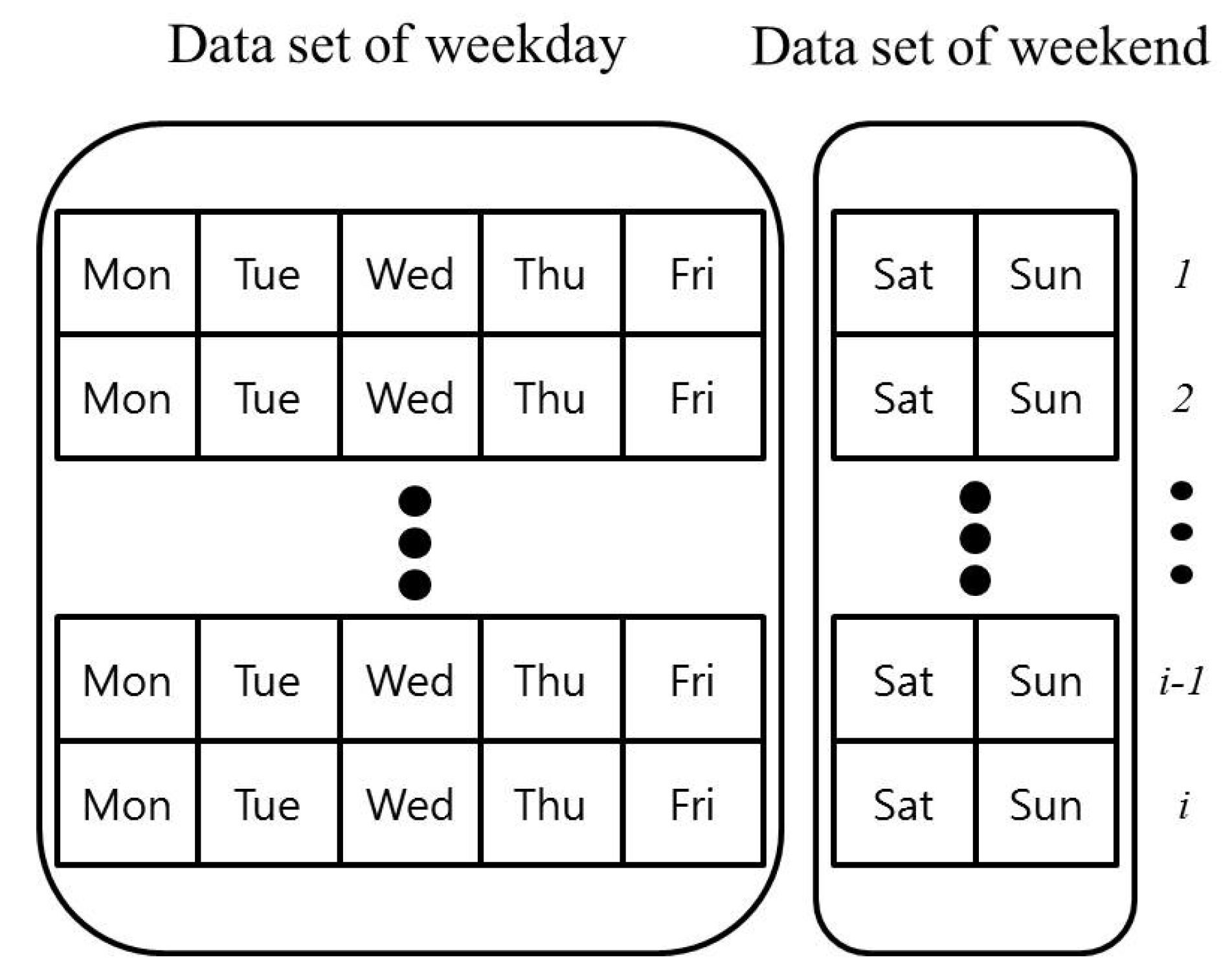
Figure 3 and Figure 4 show the load shape over 24 hours of weekdays and weekends in the building. These data were collected by Korea Energy Management Corporation (KEMCO) during March 2012 in Korea. As shown in Figure 3 and Figure 4, the graph shape differs for weekdays and weekends. Because people usually work on weekdays, the load characteristic of weekdays differs from that of the weekend: this research does not consider the holiday case on account of its irregularity. Temperature is also an influential factor. Based on the tendencies of loads due to weather and time, the input data sequences are divided as in Figure 5.

Figure 3. Sample of hourly electrical demand during the weekday.

Figure 3. Sample of hourly electrical demand during the weekday.

Figure 4. Sample of hourly electrical demand during the weekend.

Figure 4. Sample of hourly electrical demand during the weekend.

Figure 5. Sample of hourly electrical demand for i weeks.

Figure 5. Sample of hourly electrical demand for i weeks.

Thus, in the weekday case, this model uses data, including days from Monday to Friday, such as $\{mo{n}_1,tu{e}_1,we{d}_1,\cdots ,th{u}_i,fr{i}_i\}$. Similarly, the weekend case uses data composed only of Saturday and Sunday: $\{sa{t}_1,su{n}_1,\cdots ,sa{t}_i,su{n}_i\}$. The value i of the data sequence represents the ith week data. Also, each datum has a 24-hourly load datum. In this data pattern classification, we reflect the characteristic of two data by using a general load model. By using Equations (1) and (2), this general model can be expressed as:

$$\begin{array}{c}L\left(t\right)=-\begin{array}{c}(a_{1}L(t-1)+\cdots +a_{n}L(t-(24\ast j_l+k_l))\end{array}\hfill \\ \begin{array}{cccc}& & & +\begin{array}{c}(b_{1}T\left(t\right)+b_{2}T(t-1)+\cdots +b_{m}T(t-(24\ast j_u+k_u)+1))\end{array}\end{array}\hfill \\ \begin{array}{cccc}& & & +\begin{array}{c}(e\left(t\right)+c_{1}e(t-1)+\cdots +c_{r}e(t-(24\ast j_e+k_e)))\end{array}\end{array}\hfill \end{array}$$

(16)

where at any instant, t, $L\left(t\right)$ is the load; $T\left(t\right)$ is the temperature and $e\left(t\right)$ is the noise; $L(t-(24\ast j+k\left)\right)$ is the previous load at time; $24\ast j+k$, where j is a day and k is a time; Similarly, $T(t-(24\ast j+k)+1)$ and $e(t-(24\ast j+k\left)\right)$ are the previous temperature and noise at time, $24\ast j+k$, respectively. This basic load model illustrates the characteristics of weekday and weekend cases by using the categorized input data. In this paper, we define the order of the load model by the following equation:

$$\begin{array}{c}L\left(t\right)=-\begin{array}{c}{a}_{1}L(t-1)+a_{2}L(t-(24\ast 7))+a_{3}L(t-(24\ast 7+1))\end{array}\hfill \\ \begin{array}{cccc}& & & +\begin{array}{c}{b}_{1}T(t-1)+b_{2}T(t-(24\ast 7))+b_{3}T(t-(24\ast 7+1))+e\left(t\right)\end{array}\end{array}\hfill \end{array}$$

(17)

Each term of the equation is labeled as follows: $L\left(t\right)$ is the forecasted load at the next step; $L(t-1)$ is the load value one hour before on the same day; $L(t-(24\ast 7\left)\right)$ is the load during the same hour 7 days prior; $L(t-(24\ast 7+1\left)\right)$ is the load one hour before the hour of 7 days prior; $T(t-1)$, $T(t-(24\ast 7\left)\right)$ and $T(t-(24\ast 7+1\left)\right)$ follow the same rule of load term. The last term, $e\left(t\right)$, represents total noise.

3.2. Division of Input Data Sequences

Most previous studies of load forecasting only dealt with estimating parameters of the load structure. Hence, this aspect tends to face increasing accumulated error caused by changes of input data characteristics. To overcome this problem, we substitute a candidate model for the current model when accumulated error exceeds a threshold value in our model. Therefore, candidate models reduce accumulated error as a back-up model. The candidate load models used in this paper and those characters are shown in Table 1. Finding the proper threshold value is important for defining scheme characteristics. Too small of a threshold may cause unnecessary model switching, but too large of a value may not provide the desired robustness to the behavioral change in load in time. The determination of the optimal threshold value should be different for different cases and may require considerable experience. However, it may be advised to set a value with some margin, calculated when reasonably accurate forecasting performance is observed during the initial calibration period. In this research, this value is assumed to be 250 kWh. The proposed scheme also provides two operation modes in order to help determine the appropriate model. The first is an initial mode and the second is an executing mode. Details of these modes are presented in the following subsections.

Table 1. Candidate load models.

Name	Model	Note
Candidate 1	$L\left(t\right)=a_{1}L(t-1)+b_{1}T(t-1)+e\left(t\right)$	Use data, an hour ago
Candidate 2	$L\left(t\right)=a_{1}L(t-(24\ast 7))+b_{1}T(t-(24\ast 7))+e\left(t\right)$	Use data, a week ago
Candidate 3	$\begin{array}{c}L\left(t\right)=a_{1}L(t-1)+a_{2}L(t-2)+b_{1}T(t-1)+\hfill \\ b_{2}T(t-2)+e\left(t\right)\hfill \end{array}$	Use data, an hour and two hours ago

Table 1. Candidate load models.

Name	Model	Note
Candidate 1	$L\left(t\right)=a_{1}L(t-1)+b_{1}T(t-1)+e\left(t\right)$	Use data, an hour ago
Candidate 2	$L\left(t\right)=a_{1}L(t-(24\ast 7))+b_{1}T(t-(24\ast 7))+e\left(t\right)$	Use data, a week ago
Candidate 3	$\begin{array}{c}L\left(t\right)=a_{1}L(t-1)+a_{2}L(t-2)+b_{1}T(t-1)+\hfill \\ b_{2}T(t-2)+e\left(t\right)\hfill \end{array}$	Use data, an hour and two hours ago

3.2.1. Initial Mode

The initial mode of MSS aims to provide a new structure quickly. When accumulated error exceeds a threshold value, there are not enough data to select the best candidate model. Because it needs two weeks at least in order to obtain sufficient data, MSS activates training mode to reduce accumulated error until the system collects sufficient load data. As shown in Figure 6, when this mode activates, our system generates estimated load data based on past data and chooses a model randomly or empirically among a set of models. Then, the basic model for load forecasting is substituted by the structure that was selected from the candidate models. Our scheme then forecasts the next time load using this model. Although there is a possibility that the accumulated error of the selected model again reaches the critical value, the initial mode plays a role in the lack of load data.

Figure 6. Process of the initial mode.

Figure 6. Process of the initial mode.

3.2.2. Executing Mode

While the purpose of the initial mode is to provide a model quickly in the case of a lack of load data, the executing mode aims to select the most accurate of the candidate structures by using sufficient data. When this mode activates, the system starts collecting sufficient load data to estimate the model coefficient for two weeks. This mode then simulates all candidates by using collected data, as shown in Figure 7. Then, our system selects the candidate that has a minimum error. Finally, the model with the least accumulated error during this period replaces the current forecasting model. Though it takes a longer time when we have more models, this can provide the best one.

Figure 7. Process of accurate mode.

Figure 7. Process of accurate mode.

4. Simulation Studies

Simulation studies are conduced to demonstrate the efficacy of the proposed load forecasting scheme with actual hourly load data as the basic input data. By using our basic load model, the accumulated and average errors of data pattern classification are evaluated with reference to errors without the proposed classification. The proposed scheme for enhancing the model robustness is also implemented and evaluated. Simulations for two modes are carried out to evaluate performance for the same scenarios. The scenario includes a changing load characteristic so that accumulated error increases. The weather data is obtained from the Korea Meteorological Administration [21].

4.1. Data Pattern Classification

To forecast the load, initial parameters, such as $x_0$, a set of $a,b,c$ and $P_0$ in Equations (13–15) must be defined. In this simulation, we set those parameters arbitrarily. Using these parameters, load demand and temperature obtained from measuring the Kalman filter is applied to estimate coefficients of the basic load model for each data pattern classification case (Table 2).

The actual daily load for the week is shown in Figure 8. By using the above values, the forecasted loads with data pattern classification are presented in Figure 9. In particular, Figure 9 illustrates weekday and weekend cases simultaneously. Table 3 compares the performance of the models with and without data pattern classification in terms of max, min and average errors. It clearly indicates that data classification helps prevent interference between the weekday load and weekend load and improves the forecasting accuracy.

Table 2. Estimated coefficients for the load model.

	$a_1$	$a_2$	$a_3$	$b_1$	$b_2$	$b_3$	$c_1$
Weekday case	0.6626	−0.2632	0.5300	−0.0090	0.1803	−0.1357	0.0223
Weekend case	0.1136	0.1548	0.6464	−0.0218	0.0696	0.0105	−0.0207
Whole-week case	0.6052	−0.1872	0.5173	0.0090	0.1932	−0.1642	0.0078

Table 2. Estimated coefficients for the load model.

	$a_1$	$a_2$	$a_3$	$b_1$	$b_2$	$b_3$	$c_1$
Weekday case	0.6626	−0.2632	0.5300	−0.0090	0.1803	−0.1357	0.0223
Weekend case	0.1136	0.1548	0.6464	−0.0218	0.0696	0.0105	−0.0207
Whole-week case	0.6052	−0.1872	0.5173	0.0090	0.1932	−0.1642	0.0078

Figure 8. Actual load demand.

Figure 8. Actual load demand.

Figure 9. Forecasted load demand with data pattern classification.

Figure 9. Forecasted load demand with data pattern classification.

Table 3. Error performance for data pattern classification.

	Max error	Min error	Average error	Accumulated error
Included	0.9705	0.0169	0.3914	9.3928
Not included	1.3230	0.0430	0.5752	13.8044
Difference	0.3525	0.0261	0.1838	4.4116

Table 3. Error performance for data pattern classification.

	Max error	Min error	Average error	Accumulated error
Included	0.9705	0.0169	0.3914	9.3928
Not included	1.3230	0.0430	0.5752	13.8044
Difference	0.3525	0.0261	0.1838	4.4116

4.2. Performance of the Model Switching Scheme

This subsection demonstrates the performance of the MSS. It is important to note that forecasting error is unavoidable and the accumulated error tends to increase continuously. Thus, our algorithm initializes the accumulated error to an initial value every regular checking period, e.g., one week in this paper. The threshold value of accumulated error is empirically chosen to be 250 kWh. Candidate forecasting models are selected, as shown in Table 1. We then investigate numerical simulations using new weekly data in Figure 10 to address the load characteristic change.

Figure 10. Weekly load as new incoming data.

Figure 10. Weekly load as new incoming data.

When the characteristics of input data change, the accumulated error of the load model increases, as shown in Figure 11. This figure shows that accumulated error is sharply increased after characteristic change and exceeds a threshold value. Because the accumulated error exceeds the threshold value, MSS starts one of the modes to substitute for the basic load model.

In the case of the initial mode, there are not sufficient load data. Thus, the system starts generating estimated load data and chooses the first candidate randomly. In the executing mode, our system has two weeks of data. Then, this mode simulates every candidate model using those data. Figure 12 indicates the improved performance of the executing mode in the proposed scheme. In this figure, the gray area means the difference between two modes. The consequent accumulated errors for initial and executing modes are 186.78 kWh and 104.64 kWh, respectively. As you can see, executing mode is superior to the initial mode in reducing the error. However, that mode has a disadvantage, because it cannot control accumulated error for two weeks, because the current model must be used until data collection is finished. The initial mode randomly chooses one of the candidates and uses estimated load data in order to estimate the coefficient of the load model. Even though the initial mode has lower performance than the executing mode, it is a significant operation mode, because it is able to decrease accumulated error until the system collects enough load data.

Figure 11. Trend of the accumulated error.

Figure 11. Trend of the accumulated error.

Figure 12. Comparison between initial and executing modes.

Figure 12. Comparison between initial and executing modes.

5. Conclusions

To improve the accuracy and robustness of the load forecasting, this paper has presented a new load forecasting strategy incorporating data pattern classification and automatic model switching and demonstrated the enhanced performance through case studies using the real energy consumption data. Specifically, this research improved accuracy by processing the input load data in terms of daily characteristics and reinforced the robustness against the structural bias error due to any change in electricity consumption pattern in the building by allowing the forecast model change. The proposed strategy has adopted ARMAX models with the Kalman filter for estimating their parameters, because they are easily implementable on top of their proven performance in time series analysis. However, it is worth noting that the forecasting model is not limited to the ARMAX models, as this study has investigated. Several candidate models with complementary structures should work with flexible and scalable architecture and interfaces, allowing for seamless transition from one model to the other in order to improve the accuracy and robustness. Accuracy and robustness against any uncertainty this research provides should help understand the energy behavior of buildings and enable the potential savings through proper load controls and demand responses, which should contribute to the cost-effective operation and stabilization of an entire generation and distribution systems, as well.