Li-Ion Battery Charging with a Buck-Boost Power Converter for a Solar Powered Battery Management System

Abstract

This paper analyzes and simulates the Li-ion battery charging process for a solar powered battery management system. The battery is charged using a non-inverting synchronous buck-boost DC/DC power converter. The system operates in buck, buck-boost, or boost mode, according to the supply voltage conditions from the solar panels. Rapid changes in atmospheric conditions or sunlight incident angle cause supply voltage variations. This study develops an electrochemical-based equivalent circuit model for a Li-ion battery. A dynamic model for the battery charging process is then constructed based on the Li-ion battery electrochemical model and the buck-boost power converter dynamic model. The battery charging process forms a system with multiple interconnections. Characteristics, including battery charging system stability margins for each individual operating mode, are analyzed and discussed. Because of supply voltage variation, the system can switch between buck, buck-boost, and boost modes. The system is modeled as a Markov jump system to evaluate the mean square stability of the system. The MATLAB based Simulink piecewise linear electric circuit simulation tool is used to verify the battery charging model.

1. Introduction

The ability to charge batteries in the air is essential for a solar powered aircraft to remain aloft overnight. To achieve this, advanced battery management must be incorporated into aircraft power management systems. This battery management system monitors and controls the storage and delivery of solar power drawn from solar cells. Battery modules are fundamental elements of a battery management system. Compared to alternative battery technologies, Li-ion batteries offer high energy density, flexible and light-weight design, no memory effects, and a long lifespan [1,2]. These advantages make Li-ion batteries highly suitable for the next generation of electric vehicle and aerospace applications [2,3].

For solar powered systems, the terminal voltage from the solar cell panel is usually designed to be higher than the voltage required at the load terminal. Power converters for maximal power point tracking and voltage or current regulation are inserted between the solar cell panel and the load to control power flow. Although voltage at the power converter input is mostly higher than the voltage required for battery charging, in many circumstances—such as shaded solar cell panels or a high incident angle—voltage may be lower than the required minimal voltage, terminating the charging process. This wastes solar power. To maximize utilization of available solar power drawn from the solar panel, this study incorporates a buck-boost converter into the solar powered battery management system for battery charging. Many studies have investigated the analysis and design of buck-boost power converters [4,5,6,7]. In [5,6] the authors developed buck-boost converters for portable applications. In [7] a buck-boost cascaded converter for high power applications, such as fuel cell electric vehicles, was proposed.

Primary battery management functions include measurement of observable quantities (such as voltage, current, and temperature), parameter and state estimation for battery performance computations (such as state of charge and state of health calculations), and optimal control strategy and power utilization determination [8]. Battery state of charge estimation requires a reliable model to describe battery cell behavior. Dynamic models representing the operation of battery cells have been widely studied. These include equivalent circuit models [9,10,11,12,13], intelligent neural network models [14,15], and physical-based electrochemical models [16,17,18,19]. In [9], an electrical battery model capable of predicting runtime and I-V performance was proposed. The model was a blend of the Thevenin-based electrical model [20,21,22], impedance-based electrical model [23], and runtime-based electrical model [24]. In this model, a capacitor and a current-controlled current source were employed to model the SOC and runtime of the battery, a RC network was used to simulate the transient response, and a voltage-controlled voltage source was utilized to bridge SOC to open-circuit voltage of the battery. In [22], all electrochemical and electrothermal processes were approximated as uniform through the entire battery and all spatial variations of concentrations, phase distributions, and potentials ignored. With these assumptions, the battery was modeled by “bulk” parameters extracted from the experimental data. The model is suitable for virtual-prototyping of portable battery-powered system.

In equivalent circuit models, several battery parameters are required to fit a circuit model (usually RC circuit networks). The physical intuition behind the meaning of battery parameters in an equivalent circuit model is lost. However, equivalent models are useful for circuit analysis and simulation. Therefore, they are commonly used in various types of battery management systems. Based on physical first principles, electrochemical models provide a description of battery internal transport and electrochemical and thermodynamic phenomena. The resulting electrochemical models are more complex, but can be more accurate than equivalent circuit models or neural network models. Several reduced-order models have been proposed to tailor electrochemical models to real-time and control applications, including the single particle model [25,26,27], electrode average model [28,29], and frequency domain method [30].

This paper analyzes and simulates the Li-ion battery charging process for a solar powered battery management system. This study uses a non-inverting synchronous buck-boost DC/DC power converter to charge a battery. The supply voltage originates from the output of the maximal power point tracking stage which automatically adjusts the output voltage to achieve maximal power transfer from the solar cell panel. The battery charging system can operate in buck, buck-boost, or boost mode according to supply voltage condition. Supply voltage variation arises from rapid changes in atmospheric conditions or the sunlight incident angle. Based on the electrode averaged electrochemical model in [28,29], an electrochemical-based equivalent circuit model for a Li-ion battery is established. This is the first contribution of this paper. The circuit model contains a dependent voltage source and a dependent current source. The dependent voltage source represents the sum of overpotential and open circuit potential of the battery. The current source is controlled by the external charging circuit. A dynamic model for the battery charging process is then constructed based on the established equivalent circuit model and the buck-boost power converter dynamic model. This is the second contribution of the paper. The battery charging process forms a system with multiple interconnections. This paper analyzes and discusses characteristics including battery charging system stability margins for each individual operating mode. Because of supply voltage variations the system can switch between buck, buck-boost, and boost modes. The system is also modeled as a Markov jump system to evaluate the mean square stability of the system. This is the third contribution of the paper. The jump system can be used as a practical example for other research purposes such as controller design for jump system or simultaneous stabilization. The MATLAB-based Simulink piecewise linear electric circuit simulation (PLECS) tool is used to verify the battery charging model.

2. Lithium Battery Model

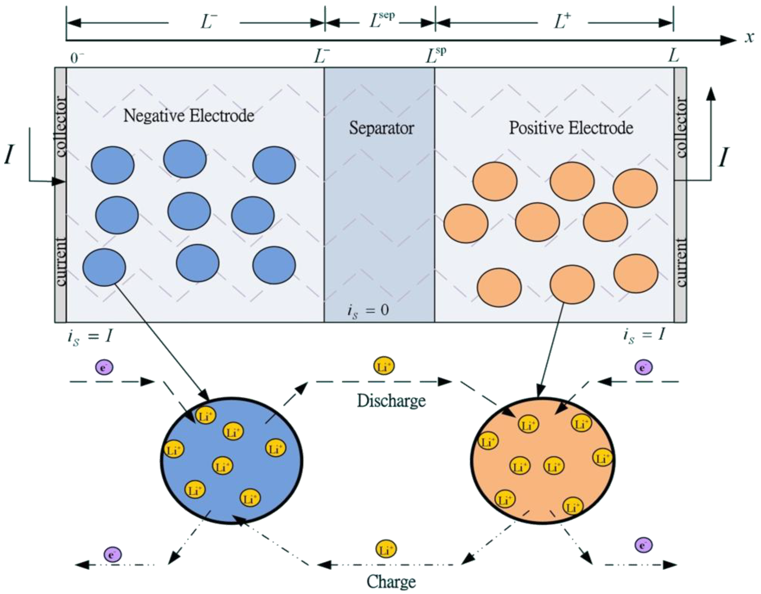
A typical Li-ion battery cell contains three main parts: a negative electrode, separator, and positive electrode, as shown in Figure 1. All three components are immersed in an electrolyte solution composed of a lithium salt in an organic solvent such as LiPF₆, LiBF₄, or LiClO₄. The negative electrode is connected to the negative terminal of the cell and usually contains graphite. The positive electrode is connected to the positive terminal of the cell and is a metal oxide or a blend of several metal oxides such as Li_xMn₂O₄ and Li_xCoO₂. The separator is a solid or liquid solution with a high concentration of lithium ions. It is an electrical insulator that prevents electrons from flowing between negative and positive electrodes, but the electrolyte allows ions to pass through it. In the discharging process, the lithium ions at the surface of the solid active material of the porous negative electrode undergo an electrochemical reaction, transferring the ions to the solution and the electrons to the negative terminal. The positive ions travel through the electrolyte solution to the positive electrode where they react with, diffuse toward, and are inserted into the metal oxide solid particles. Ions and electrons reverse traveling direction in the charging process.

Electrochemical-based models are reasonable predictors of Li-ion battery performance and physical limitations for a wide range of operating conditions [18]. However, the model contains coupled nonlinear partial differential equations that make it difficult for onboard applications. Thus, model reduction is necessary for real-time and control applications. Based on porous electrode theory [16], Li-ions can exist in a solid phase (intercalated in the electrode material) or an electrolyte phase in a dissolved state. The porous structure can be interpreted as consisting of small spherical solid particles, as shown in Figure 1.

Figure 1. Structure of a Li-ion battery cell.

Figure 1. Structure of a Li-ion battery cell.

For simplicity and computational tractability, one-dimensional spatial models [17,18,19] are widely used in battery performance analysis and state of charge estimation. State variables required to one to describe electrochemical behavior while charging or discharging a lithium battery include electric potential ${\Phi }_{\mathrm{s}}$ in the solid electrode, electric potential ${\Phi }_{\mathrm{e}}$ in the electrolyte, current $i_{\text{s}}$ in the solid electrode, current $i_{\text{e}}$ in the electrolyte, concentration $c_{\text{s}}$ of lithium in the solid phase, concentration $c_{\text{e}}$ of the electrolyte salt, and molar flux $j_{\text{n}}$ of lithium at the surface of the spherical particle. Assuming that battery discharging current is $I$ and plate area is $A$, the governing equations that describe the electrochemical behavior of the battery and the relationship between state variables and input/output signals of the model are summarized below.

Potential variation in the solid electrode along the x-axis is described by:

$$\frac{\partial {\text{Φ}}_s}{\partial x}=-\frac{i_{\text{s}}}{\sigma }=\frac{i_{\text{e}}-I/A}{\sigma }$$

(1)

where s is the effective electronic conductivity of the electrode. The relationship between potential and current in the electrolyte is calculated using:

$$\frac{\partial {\text{Φ}}_{\mathrm{e}}}{\partial x}=-\frac{i_{\text{e}}}{\kappa }+\frac{2RT}{F}\left(1-t_{+}^0\right)\frac{\partial \text{ln}{c}_{\text{e}}}{\partial x}$$

(2)

where $R$ is the universal gas constant, $T$ is temperature ($K$), $F$ is Faraday’s constant, $\kappa$ is the ionic conductivity of the electrolyte, and $t_{+}^0$ is the transference number of the positive ions with respect to solvent velocity. Lithium concentration variation in the electrolyte is calculated using:

$$\epsilon \frac{\partial c_{\text{e}}}{\partial t}=\frac{\partial }{\partial x}\left(\epsilon D_{\text{e}}\frac{\partial c_{\text{e}}}{\partial x}\right)+\left(1-t_{+}^0\right)\frac{j^{L_i}}{F}$$

(3)

where $D_{\text{e}}$ is the effective diffusion coefficient, $\epsilon$ is the volume fraction of the electrolyte, and $j^{L_i}$ is the lithium ion flux. Variable $j^{L_i}$ is defined as:

$$\frac{\partial i_e}{\partial x}=aF{j}_n=j^{L_i}$$

(4)

where $a$ is the superficial area per electrode volume unit. Lithium ion transport in the electrode is described by:

$$\frac{\partial c_{\text{s}}}{\partial t}=\frac{1}{r^2}\frac{\partial }{\partial r}\left(D_{\text{s}}{r}^2\frac{\partial c_{\text{s}}}{\partial r}\right)$$

(5)

where r is the radial dimension of electrode particles and $D_{\text{s}}$ is the diffusion coefficient. The corresponding boundary conditions are:

$${\frac{\partial c_{\text{s}}}{\partial r}|}_{r=0}=0\text{ and }{\frac{\partial c_{\text{s}}}{\partial r}|}_{r=R_{\text{p}}}=-\frac{1}{D_{\text{s}}aF}{j}^{L_i}$$

(6)

Governing Equations (1), (2), (3), and (5) describing the behavior of the state variables ${\text{Φ}}_{\mathrm{s}}$, ${\text{Φ}}_{\mathrm{e}}$, $c_{\text{e}}$, and $c_{\text{s}}$ are coupled through the Butler-Volmer electrochemical kinetic equation:

$$j^{L_i}=a{i}_{\text{o}}\left[\text{exp}\left(\frac{{\alpha }_{a}F}{RT}\eta \right)-\exp \left(\frac{{\alpha }_{c}F}{RT}\eta \right)\right]$$

(7)

where ${\alpha }_a$ and ${\alpha }_c$ are the anodic and cathodic transport coefficients, respectively, $i_{\text{o}}$ is the exchange current density, and $\eta$ is the surface overpotential. Surface overpotential $\eta$ is the driving force of (5) and is defined as the difference between solid state and electrolyte phase potentials minus thermodynamic equilibrium potential $U$ of the solid phase. Mathematically, $\eta$ is expressed as:

$$\eta ={\text{Φ}}_{\mathrm{s}}-{\text{Φ}}_{\mathrm{e}}-U\left(c_{\text{ss}}\right)$$

(8)

where equilibrium potential $U(c_{\text{ss}})$ is evaluated as a function of the solid phase concentration at the particle surface and $c_{\text{ss}}$ is the lithium ion concentration at the solid particle surface. Exchange current density $i_{\text{o}}$ is related to the solid surface and electrolyte concentration and is calculated using:

$$i_{\text{o}}=F{r}_k{\left(c_{\text{s},\text{max}}-c_{\text{ss}}\right)}^{{\alpha }_c}{\left(c_{\text{ss}}\right)}^{{\alpha }_c}{\left(c_{\text{e}}\right)}^{{\alpha }_a}$$

(9)

where $r_{\text{k}}$ is the rate constant and $c_{\text{s},\text{max}}$ is the maximal possible concentration of lithium in the solid particles of the electrode based on material properties.

In the electrode solid concentration model, the spatial solid concentration distribution along the x coordinate is ignored (i.e., diffusion between adjacent particles is ignored). Diffusion dynamics along the r coordinate are only considered inside a representative particle. To simplify the analysis, the spherical particle with radius $R_{\text{p}}$ is divided into $M_{\text{r}}$ slices, $\text{Δ}r=R_{\text{p}}/M_{\text{r}}$ in size. Let the solid concentration at radial coordinate $\text{Δ}r\cdot q$, $q=1,2\cdots ,M_{\text{r}-1}$, be $c_{\text{sq}}$, and select $c_{\text{s}}={\left[c_{\text{sq}}\right]}^T$ as the state vector. Concentration $c_{\text{s}0}$ (concentration at the particle center) is excluded from the state vector because it is constrained by the first initial condition in (6). The other boundary condition for $r=R_{\text{p}}$ (surface concentration $c_{{\text{sM}}_{\text{r}}}=c_{\text{ss}}$) is also excluded from the state vector. Concentration $c_{\text{ss}}$ can be obtained from the second boundary condition in (6) and can be estimated using:

$$c_{\text{ss}}=c_{{\text{sM}}_{\text{r}}-1}+{\displaystyle {\int }_{(M_{\text{r}}-1)\text{Δ}r}^{M_{\text{r}}\text{Δ}r}\frac{\partial c_{\text{s}}}{\partial r}}dr\simeq c_{{\text{sM}}_{\text{r}}-1}-\frac{\text{Δ}r}{D_{\text{s}}aF}{j}^{L_i}$$

(10)

PDE (5) can be approximated using the finite differences and (11):

$$\begin{array}{c}{\dot{c}}_{\text{sq}}=D_{\text{s}}\left[\frac{2}{q\text{Δ}r}\frac{c_{\text{s}(\text{q}+1)}-c_{\text{s}(\text{q}-1)}}{2\text{Δ}r}+\frac{c_{\text{s}(\text{q}+1)}-2c_{\text{sq}}+c_{\text{s}(\text{q}-1)}}{{(\text{Δ}r)}^2}\right]\\ =\frac{D_{\text{s}}}{{(\text{Δ}r)}^2}\left[\frac{q+1}{q}{c}_{\text{s}(\text{q}+1)}-2c_{\text{sq}}+\frac{q-1}{q}{c}_{\text{s}(\text{q}-1)}\right]\end{array}$$

(11)

Using (10), state Equation (11) for $q=M_{\text{r}}-1$ is rewritten as:

$$\begin{array}{c}{\dot{c}}_{\text{s}({\text{M}}_{\mathrm{r}}-1)}=\frac{D_{\text{s}}}{{(\text{Δ}r)}^2}\left[\frac{M_{\text{r}}}{M_{\text{r}}-1}\left(c_{\text{s}({\text{M}}_{\mathrm{r}}-1)}-\frac{\text{Δ}r}{D_{\text{s}}aF}{j}^{Li}\right)-2c_{\text{s}({\text{M}}_{\mathrm{r}}-1)}+\frac{M_{\text{r}}-2}{M_{\text{r}}-1}{c}_{\text{s}({\text{M}}_{\mathrm{r}}-2)}\right]\\ =\frac{D_{\text{s}}}{{(\text{Δ}r)}^2}\frac{M_{\text{r}}-2}{M_{\text{r}}-1}\left[c_{\text{s}({\text{M}}_{\mathrm{r}}-2)}-c_{\text{s}({\text{M}}_{\mathrm{r}}-1)}\right]-\frac{M_{\text{r}}}{M_{\text{r}}-1}\frac{1}{aF\text{Δ}r}{j}^{Li}\end{array}$$

(12)

State Equations (11) and (12) represent the approximate solid concentration distribution dynamics of a particular solid particle inside the electrode. To facilitate analysis and control and estimation applications, this study uses the electrode averaged model [28,29] for solid concentration distribution dynamics for battery charging analysis and design. In addition it neglects the solid concentration distribution along the electrodes, so the electrode averaged model only considers material diffusion inside a representative solid material particle (one for each electrode) and averages the state and input variables in the model. The model assumes that electrolyte concentration is constant (which is reasonable for a highly concentrated electrolyte). The electrode averaged model was first reviewed. The results were then used to construct an electrochemical-based equivalent circuit model for battery charging analysis and simulation.

In the electrode averaged model, average solid concentration dynamics are driven by constant flux (the average value of $j^{Li}$) ${\overline{j}}^{Li}$. The average value of $j^{Li}$ along the negative electrode is:

$${\overline{j}}_{\text{n}}^{Li}=\frac{1}{L^{-}}{\displaystyle {\int }_0^{L^{-}}{j}_{\text{n}}^{Li}}d\overline{x}=\frac{1}{L^{-}}{\displaystyle {\int }_0^{L^{-}}\frac{\partial i_{\text{e}}(\overline{x})}{\partial \overline{x}}}d\overline{x}=\frac{I}{A{L}^{-}}$$

(13)

The average value of $j^{Li}$ along the positive electrode, ${\overline{j}}_{\text{p}}^{Li}$, is calculated using:

$${\overline{j}}_{\text{p}}^{Li}=\frac{1}{L^{+}}{\displaystyle {\int }_{L^{\text{sp}}}^L{j}_{\text{p}}^{Li}}d\overline{x}=\frac{1}{L^{+}}{\displaystyle {\int }_{L^{\text{sp}}}^{L^{+}}\frac{\partial i_{\text{e}}(\overline{x})}{\partial \overline{x}}}d\overline{x}=\frac{1}{L^{+}}{i_e|}_{L^{\text{sp}}}^L=\frac{-I}{A{L}^{+}}$$

(14)

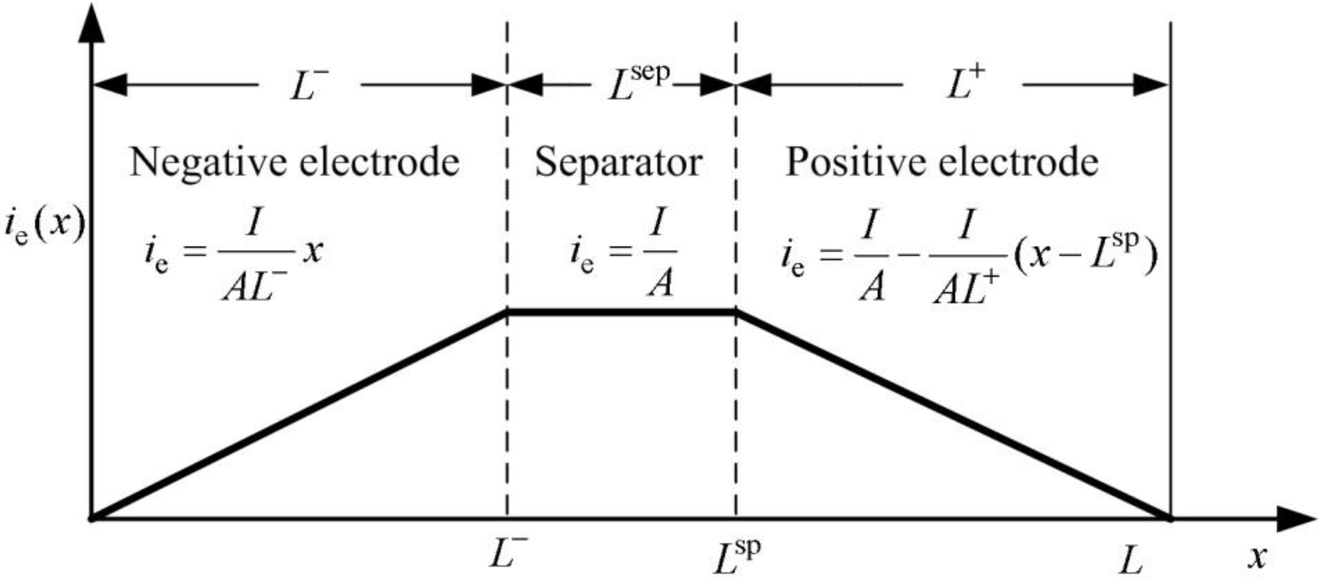
Using ${\overline{j}}_{\text{n}}^{Li}$, ${\overline{j}}_{\text{p}}^{Li}$, the conservation of charge from (4), and appropriate boundary conditions, current density $i_{\text{e}}$ becomes piecewise linear proportional to $x$, as shown in Figure 2.

Figure 2. Distribution of current density in electrolyte.

Figure 2. Distribution of current density in electrolyte.

Using Figure 2 and (2) and assuming that $c_{\text{e}}$ is constant, the potential in the electrolyte for negative electrode $0\le x\le L^{-}$ is:

$${\text{Φ}}_{\mathrm{e}}\text{(}x)={\text{Φ}}_{\mathrm{e}}(0)+{\displaystyle {\int }_0^x\frac{\partial {\text{Φ}}_{\mathrm{e}}(\overline{x})}{\partial \overline{x}}d\overline{x}}={\text{Φ}}_e(0)-{\displaystyle {\int }_0^x\frac{i_{\text{e}}(\overline{x})}{{\kappa }_{\text{n}}}d\overline{x}}={\text{Φ}}_{\mathrm{e}}(0)-\frac{I}{2A{L}^{-}{\kappa }_{\text{n}}}{x}^2$$

(15)

Potential ${\text{Φ}}_{\mathrm{e}}$ for separator $L^{-}\le x\le L^{\text{sp}}$ is:

$${\text{Φ}}_{\mathrm{e}}(x)={\text{Φ}}_{\mathrm{e}}(0)-\frac{I}{2A{\kappa }_{\text{n}}}{L}^{-}-\frac{I}{A{\kappa }_{\text{sep}}}(x-L_{\text{sp}})$$

(16)

Similarly, potential ${\text{Φ}}_{\mathrm{e}}$ for positive electrode $L^{\text{sp}}\le x\le L$ is:

$${\text{Φ}}_{\mathrm{e}}(x)={\text{Φ}}_{\mathrm{e}}(0)-\frac{I}{2A{\kappa }_{\text{n}}}{L}^{-}-\frac{I}{A{\kappa }_{\text{sep}}}{L}^{sep}-\frac{I}{A{\kappa }_{\text{p}}}\left[\left(x-L_{\text{sp}}\right)-\frac{{\left(x-L_{\text{sp}}\right)}^2}{2L^{+}}\right]$$

(17)

Thus, using external applied current I as the input and average solid concentration as the state variable, the average solid concentration distribution dynamics inside the negative and positive solid particles are expressed using (18) and (19), respectively:

$${\dot{\overline{c}}}_{\text{sn}}=A_{\text{n}}{\overline{c}}_{\text{sn}}+B_{\text{n}}I, {\overline{c}}_{\text{ssn}}=C_{\text{n}}{\overline{c}}_{\text{sn}}+D_{\text{n}}I$$

(18)

$${\dot{\overline{c}}}_{\text{sp}}=A_{\text{p}}{\overline{c}}_{\text{sp}}+B_{\text{p}}I, {\overline{c}}_{\text{ssp}}=C_{\text{p}}{\overline{c}}_{\text{sp}}+D_{\text{p}}I$$

(19)

where:

$$\begin{array}{l}{\dot{\overline{c}}}_{\text{sn}}={\left[\begin{array}{ccccc}{\overline{c}}_{\text{sn}1}& {\overline{c}}_{\text{sn}2}& \cdots & {\overline{c}}_{\text{sn}(M_{{\text{r}}_{\mathrm{n}}}-2)}& {\overline{c}}_{\text{sn}(M_{{\text{r}}_{\mathrm{n}}}-1)}\end{array}\right]}^T\\ A_{\text{n}}=\frac{D_{\text{s},\text{n}}}{{(\text{Δ}{r}_{\text{n}})}^2}\left[\begin{array}{cccccccc}-2& 2& 0& 0& \cdots & 0& & \\ 1/2& -2& 3/2& 0& \cdots & & & \\ ⋮& & & & \ddots & & & ⋮\\ 0& \cdots & & & 0& \frac{M_{{\text{r}}_{\mathrm{n}}}-3}{M_{{\text{r}}_{\mathrm{n}}}-2}& -2& \frac{M_{{\text{r}}_{\mathrm{n}}}-1}{M_{{\text{r}}_{\mathrm{n}}}-2}\\ 0& \cdots & & & 0& 0& \frac{M_{{\text{r}}_{\mathrm{n}}}-2}{M_{{\text{r}}_{\mathrm{n}}}-1}& -\frac{M_{{\text{r}}_{\mathrm{n}}}-2}{M_{{\text{r}}_{\mathrm{n}}}-1}\end{array}\right]\\ B_{\text{n}}={\left[\begin{array}{ccccc}0& 0& \cdots & 0& -\left(\frac{M_{{\text{r}}_{\mathrm{n}}}}{M_{{\text{r}}_{\mathrm{n}}}-1}\frac{1}{a_{\text{n}}F\text{Δ}{r}_{\text{n}}}\frac{1}{A{L}^{-}}\right)\end{array}\right]}^T\\ C_{\text{n}}=\left[\begin{array}{ccccc}0& 0& \cdots & 0& 1\end{array}\right] , D_{\text{n}}=-\frac{\text{Δ}{r}_{\text{n}}}{D_{\text{s},\text{n}}{a}_{\text{n}}FA{L}^{-}}\end{array}$$

(20)

and:

$$\begin{array}{l}{\dot{\overline{c}}}_{\text{sp}}={\left[\begin{array}{ccccc}{\overline{c}}_{\text{sp}1}& {\overline{c}}_{\text{sp}2}& \cdots & {\overline{c}}_{\text{sp}(M_{{\text{r}}_{\mathrm{n}}}-2)}& {\overline{c}}_{\text{sp}(M_{{\text{r}}_{\mathrm{n}}}-1)}\end{array}\right]}^T\\ A_{\text{p}}=\frac{D_{\text{s},\text{p}}}{{(\text{Δ}{r}_{\text{n}})}^2}\left[\begin{array}{cccccccc}-2& 2& 0& 0& \cdots & & & 0\\ 1/2& -2& 3/2& 0& \cdots & & & \\ ⋮& & & & \ddots & & & ⋮\\ 0& \cdots & & & 0& \frac{M_{{\text{r}}_{\mathrm{n}}}-3}{M_{{\text{r}}_{\mathrm{n}}}-2}& -2& \frac{M_{{\text{r}}_{\mathrm{n}}}-1}{M_{\text{r}}-2}\\ 0& \cdots & & & 0& 0& \frac{M_{{\text{r}}_{\mathrm{n}}}-2}{M_{{\text{r}}_{\mathrm{n}}}-1}& -\frac{M_{{\text{r}}_{\mathrm{n}}}-2}{M_{{\text{r}}_{\mathrm{n}}}-1}\end{array}\right]\\ B_{\text{p}}={\left[\begin{array}{ccccc}0& 0& \cdots & 0& \left(\frac{M_{{\text{r}}_{\mathrm{n}}}}{M_{{\text{r}}_{\mathrm{n}}}-1}\frac{1}{a_{\text{p}}F\text{Δ}{r}_{\text{n}}}\frac{1}{A{L}^{+}}\right)\end{array}\right]}^T\\ C_{\text{p}}=\left[\begin{array}{ccccc}0& 0& \cdots & 0& 1\end{array}\right] , D_{\text{p}}=\frac{\text{Δ}{r}_{\text{n}}}{D_{\text{s},\text{p}}{a}_{\text{p}}FA{L}^{+}}\end{array}$$

(21)

Battery voltage is calculated using:

$$V_{\text{BATT}}={\text{Φ}}_{\mathrm{s}}(L)-{\text{Φ}}_{\mathrm{s}}(0)-R_{\text{f}}I$$

(22)

where $R_{\text{f}}$ is the film resistance on the electrode surface. Battery voltage, using overpotential from (8), is characterized using the following equation:

$$V_{\text{BATT}}={\eta }_{\text{p}}(L)-{\eta }_{\text{n}}(0)+{\text{Φ}}_{\mathrm{e}}(L)-{\text{Φ}}_{\mathrm{e}}(0)+U_{\text{p}}(c_{\text{ss}}(L))-U_{\text{n}}(c_{\text{ss}}(0))-R_{\text{f}}I$$

(23)

From (17), using the averaged expression and assuming the ionic conductivity of the electrolyte in negative, positive, and separation regions are the same (i.e., ${\kappa }_{\text{n}}={\kappa }_{\text{p}}={\kappa }_{\text{sep}}=\kappa$) , potential differences ${\text{Φ}}_{\mathrm{e}}(L)-{\text{Φ}}_{\mathrm{e}}(0)$ can be calculated using:

$${\text{Φ}}_{\mathrm{e}}(L)-{\text{Φ}}_{\mathrm{e}}(0)=-\left(\frac{L^{-}+2L^{\text{sep}}+L^{+}}{2A\kappa }\right)\cdot I$$

(24)

Averaged overpotentials ${\overline{\eta }}_{\text{n}}$ and ${\overline{\eta }}_{\text{p}}$ are obtained by using (7) to produce (25) and (26):

$${\overline{\eta }}_{\text{n}}=\frac{RT}{\alpha F}\text{ln}\left({\xi }_{\text{n}}+\sqrt{{\xi }_{\text{n}}^2+1}\right), {\xi }_{\text{n}}=\frac{I}{2a_{\text{n}}{i}_{\text{o},\text{n}}A{L}^{-}}$$

(25)

$${\overline{\eta }}_{\text{p}}=\frac{RT}{\alpha F}\text{ln}\left({\xi }_{\text{p}}+\sqrt{{\xi }_{\text{p}}^2+1}\right), {\xi }_{\text{p}}=\frac{-I}{2a_{\text{p}}{i}_{\text{o},\text{p}}A{L}^{+}}$$

(26)

The battery voltage using the electrode averaged model is characterized in the following form:

$$\begin{array}{c}{V}_{\text{BATT}}=U_{\text{p}}({\overline{c}}_{\text{ss},\text{p}})-U_{\text{n}}({\overline{c}}_{\text{ss},\text{n}})+{\overline{\eta }}_{\text{p}}-{\overline{\eta }}_{\text{n}}-\left(\frac{L^{-}+2L^{\text{sep}}+L^{+}}{2A\kappa }+R_{\text{f}}\right)\cdot I\\ =V_{\text{OCP}}({\overline{c}}_{\text{ss}})+V_{\text{OVP}}({\overline{c}}_{\text{ss}},I)-V_{\text{R}}(I)\end{array}$$

(27)

where:

$$\begin{array}{c}{V}_{\text{OCP}}({\overline{c}}_{\text{ss}})=U_{\text{p}}({\overline{c}}_{\text{ss},\text{p}})-U_{\text{n}}({\overline{c}}_{\text{ss},\text{n}})\\ V_{\text{OVP}}({\overline{c}}_{\text{ss}},I)={\overline{\eta }}_{\text{p}}-{\overline{\eta }}_{\text{n}}=\frac{RT}{\alpha F}\text{ln}\left({\xi }_{\text{p}}+\sqrt{{\xi }_{\text{p}}^2+1}\right)-\frac{RT}{\alpha F}\text{ln}\left({\xi }_{\text{n}}+\sqrt{{\xi }_{\text{n}}^2+1}\right)\\ V_{\text{R}}(I)=\left[\frac{L^{-}+2L^{\text{sep}}+L^{+}}{2A\kappa }+R_{\text{f}}\right]\cdot I=R_{\text{B}}\cdot I\end{array}$$

(28)

Voltage $V_{\text{OCP}}$, also called open circuit potential, depends only on the solid concentration ${\overline{c}}_{\text{ss}}$. Voltage $V_{\text{OVP}}$ is the output from overpotential difference ${\overline{\eta }}_{\text{p}}-{\overline{\eta }}_{\text{n}}$. It depends on concentration ${\overline{c}}_{\text{ss}}$ and the external applied current. Voltage $V_{\text{OVP}}$ is zero if applied current is removed. Voltage $V_{\text{R}}$ accounts for overall film resistance on the electrode surface and ionic resistance for the electrolyte. If applied current is removed, voltage $V_{\text{R}}$ is zero.

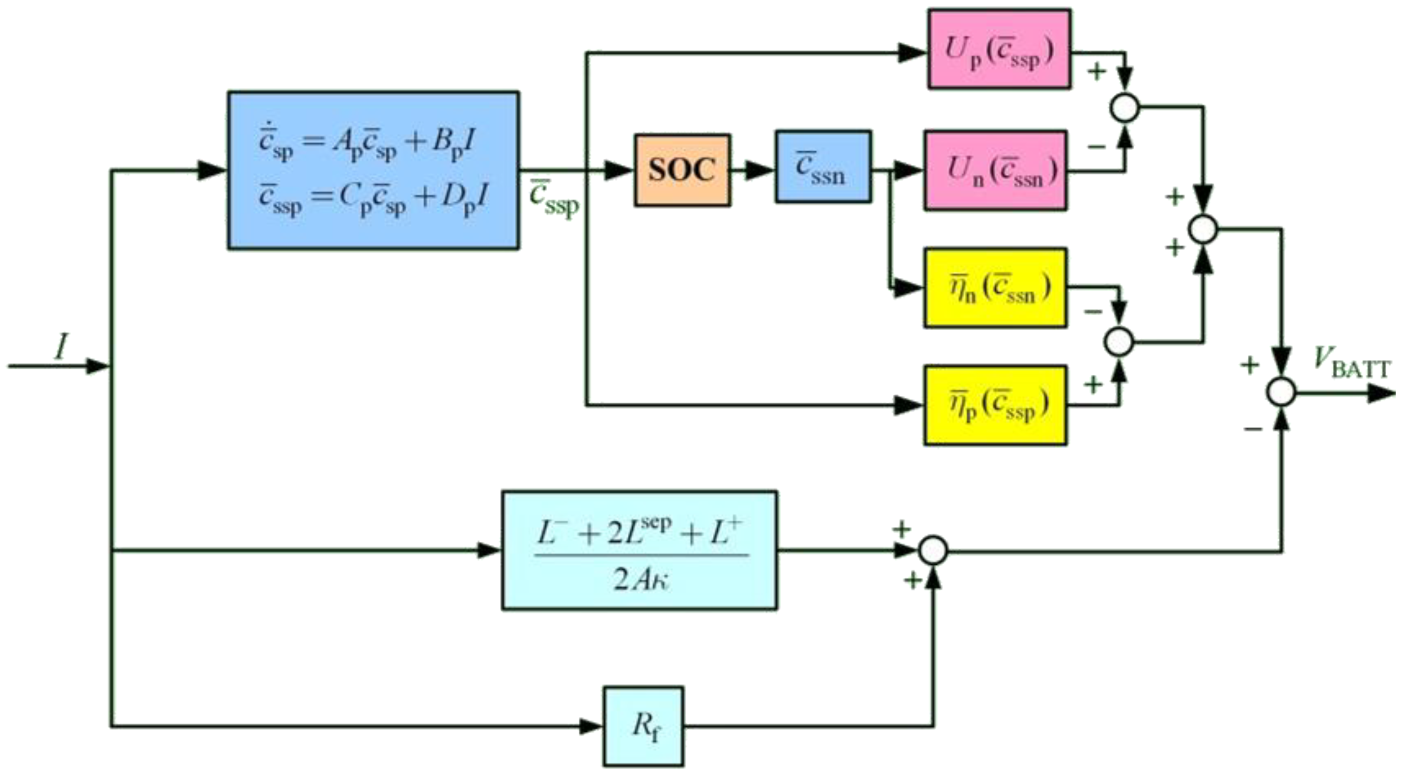
Surface concentrations for the positive and negative electrodes are first determined using the electrode averaged model. Surface concentration information and applied current are used to obtain open circuit potential $V_{\text{OCP}}$, overpotential difference $V_{\text{OVP}}$, and resistance dependent voltage $V_{\text{R}}$. Battery voltage is then calculated using (27). For practical applications, these solid concentrations must be adjusted using a state estimation algorithm (such as Kalman filtering) before they can be used to predict the state of charge (SOC) available for discharge. However, battery model output depends on open circuit potential $U_{\text{p}}({\overline{c}}_{\text{ss},\text{p}})-U_{\text{n}}({\overline{c}}_{\text{ss},\text{n}})$, not open circuit potential $U_{\text{p}}({\overline{c}}_{\text{ss},\text{p}})$ or $U_{\text{n}}({\overline{c}}_{\text{ss},\text{n}})$. That is, a system which includes positive and negative electrode states is weakly observable from the battery voltage output. Only considering the solid concentration dynamics of the positive electrode can improve this. The surface concentration of the negative electrode is estimated by determining the SOC by introducing utilization ratio ${\theta }_{\text{p}}$ from the positive electrode. Utilization ratio ${\theta }_{\text{p}}$ is defined as:

$${\theta }_{\text{p}}=\frac{{\overline{c}}_{\text{sbp}}}{c_{\text{sp},\text{max}}}, {\theta }_{\text{p}100\%}\le {\theta }_p\le {\theta }_{\text{p}0\%}$$

(29)

where ${\overline{c}}_{\text{sbp}}$ is the average bulk positive solid concentration and ${\theta }_{\text{p}0\%}$ and ${\theta }_{\text{p}100\%}$ are the average concentrations for a fully discharged and charged battery, respectively. Utilization ratios ${\theta }_{\text{p}0\%}$ and ${\theta }_{\text{p}100\%}$ are related to battery capacity $Q$ and are characterized using:

$$\left|{\theta }_{\text{p}100\%}-{\theta }_{\text{p}0\%}\right|=\frac{Q}{A{L}^{+}F{\epsilon }_{\text{sp}}{c}_{\text{sp},\text{max}}}$$

(30)

where ${\epsilon }_{\text{sp}}$ is the volume fraction of active material in the positive electrode. The SOC determined from the positive electrode is assumed to vary linearly with ${\theta }_{\text{p}}$ and is expressed as [31]:

$$\text{SOC}=\frac{{\theta }_{\text{p}}-{\theta }_{\text{p}0\%}}{{\theta }_{\text{p}100\%}-{\theta }_{\text{p}0\%}}$$

(31)

The SOC estimation must account for both positive and negative electrodes. Thus, it can be assumed that the SOC associated with utilization ratio ${\theta }_{\text{n}}$ for the negative electrode is the same as the SOC obtained from the positive electrode at any point. That is, utilization ratio ${\theta }_{\text{n}}$ is calculated using:

$${\theta }_{\text{n}}={\theta }_{\text{n}0\%}+\text{SOC}({\theta }_{\text{n}100\%}-{\theta }_{\text{n}0\%}) , {\theta }_{\text{n}0\%}\le {\theta }_{\text{n}}\le {\theta }_{\text{n}100\%}$$

(32)

Utilization ratio ${\theta }_{\text{n}}$ is used to calculate average bulk concentration for the negative electrode ${\overline{c}}_{\text{sbn}}$:

$${\overline{c}}_{\text{sbn}}={\theta }_{\text{n}}\cdot c_{\text{sn},\text{max}}$$

(33)

Surface solid concentration ${\overline{c}}_{\text{ssn}}$ for the negative electrode can then be estimated using:

$${\overline{c}}_{\text{ssn}}={\overline{c}}_{\text{sbn}}-\frac{\text{Δ}{r}_{\text{n}}}{D_{\text{s},\text{n}}{a}_{\text{n}}FA{L}^{-}}\cdot I$$

(34)

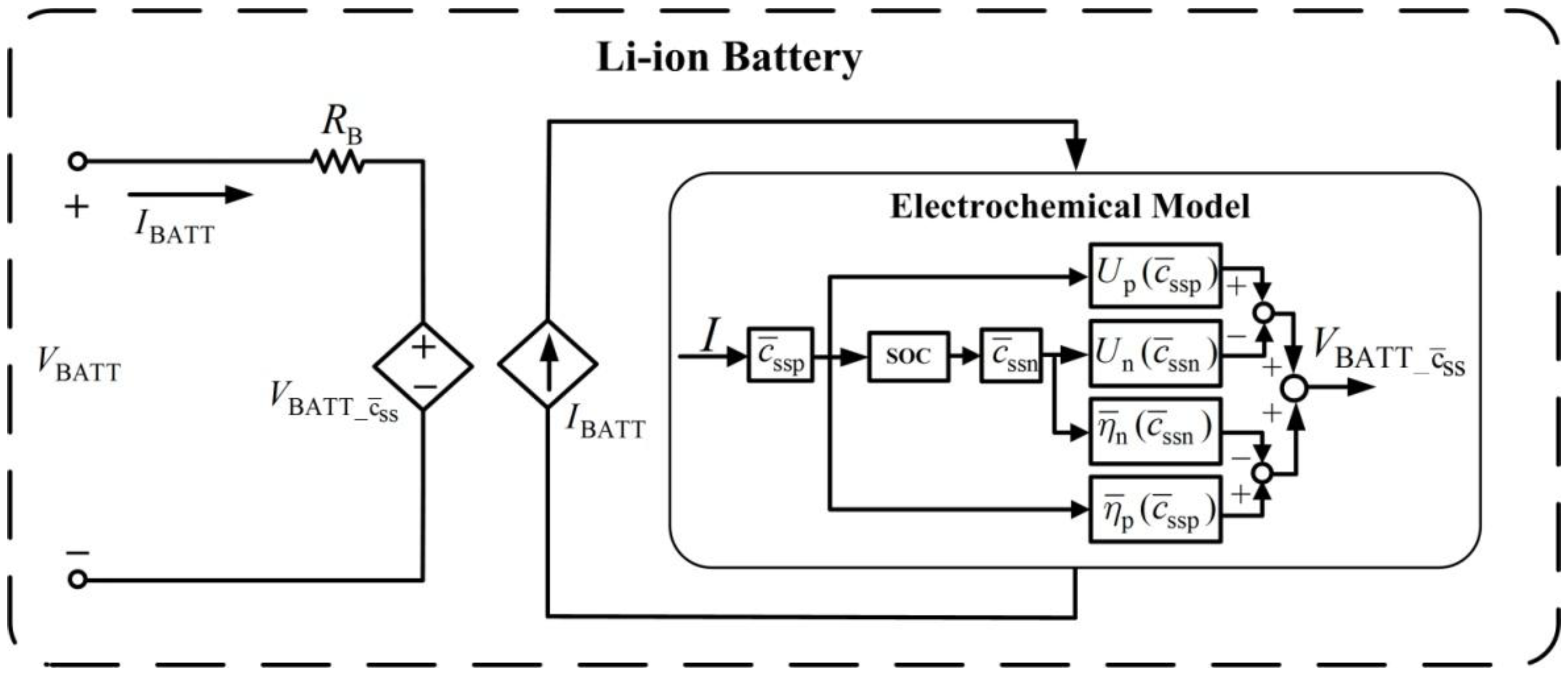
Figure 3 shows the battery model which only includes solid concentration states for the positive electrode.

Figure 3. Electrochemical based Li-ion battery model.

Figure 3. Electrochemical based Li-ion battery model.

The battery voltage characteristics in (27) are used to establish an equivalent circuit model, as shown in Figure 4. The circuit model contains a dependent voltage source, $V_{{\text{BATT\_}\overline{\text{c}}}_{\text{ss}}}$, and a dependent current source, $I_{\text{BATT}}$. Dependent voltage source $V_{{\text{BATT\_}\overline{\text{c}}}_{\text{ss}}}$ represents the sum of overpotential $V_{\text{OVPD}}$ and open circuit potential $V_{\text{OCP}}$. The current source $I_{\text{BATT}}$ is controlled by the external charging circuit. This study uses this circuit for battery charging analysis.

Figure 4. Equivalent circuit model for the Li-ion battery.

Figure 4. Equivalent circuit model for the Li-ion battery.

3. Synchronous Buck-Boost Converter

The non-inverting buck-boost converter can convert the source supply voltage higher and lower voltages to the load terminal while leaving voltage polarity unchanged. Figure 5 shows a diagram of the synchronous buck-boost circuit. Four high speed power MOSFETs ($Q_1~Q_4$) are used to control energy flow from the supply to load terminals.

Figure 5. Synchronous non-inverting buck-boost power converter.

Figure 5. Synchronous non-inverting buck-boost power converter.

Because of supply voltage variations, the power converter operates in buck, buck-boost, or boost modes through proper control of the power MOSFETs. When supply voltage is higher than the desired load voltage, the converter is set to buck operation. In buck mode operation, transistor $Q_4$ is always on and $Q_3$ is always off. Buck mode operation is achieved by controlling power switches $Q_1$ and $Q_2$. When transistor $Q_1$ is closed and $Q_2$ is open, the power source charges the inductor. In the inductor charging cycle, inductor current increases almost linearly and the capacitor supplies output current to the load. For inductor discharging, transistor $Q_2$ is closed and transistor $Q_1$ is open. In this mode, energy stored in the inductor is delivered to the capacitor (charging the capacitor) and the load. Current from the inductor decreases almost linearly during the inductor discharge period. If the duty cycle for charging the inductor is $d$, average load voltage $V_{\text{out}}$ equals $d{V}_S$ for buck operation. Duty cycle d < 1, thus, controlling duty cycle $d$ regulates output voltage $V_{\text{out}}$ at a voltage less than supplied voltage $V_S$.

When the supply voltage is less than the desired load voltage, the converter is set to boost operation. In boost mode operation, transistor $Q_1$ is on and $Q_2$ is off. To charge the inductor, transistor $Q_3$ is closed and $Q_4$ is open. The operation of $Q_3$ and $Q_4$ are reversed during the inductor discharge cycle. In boost mode, average load voltage $V_{\text{out}}$ equals 1/(1 − d)V_S. Thus, the output voltage can be higher than the input supply voltage. When supply voltage is close to the desired load voltage, the converter is set to buck-boost operation. In this mode, transistors $Q_1$ and $Q_3$ work as a group and $Q_2$ and $Q_4$ work as another group. To charge the inductor, switches $Q_1$ and $Q_3$ are closed and $Q_2$ and $Q_4$ are open. Transistors $Q_2$ and $Q_4$ are closed and $Q_1$ and $Q_3$ are opened to engage the inductor discharge cycle. In this mode, average load voltage $V_{\text{out}}$ equals d/(1 − d)V_S. This implies that output voltage can be changed to more or less than the supplied voltage. Table 1 shows a summary of power converter operation.

Table 1. Summaries of the operation of the buck-boost converter.

		Buck mode	Buck-Boost mode	Boost mode
$Q_1$	Inductor charge	ON	ON	ON
	Inductor discharge	OFF	OFF	ON
$Q_2$	Inductor charge	OFF	OFF	OFF
	Inductor discharge	ON	ON	OFF
$Q_3$	Inductor charge	OFF	ON	ON
	Inductor discharge	OFF	OFF	OFF
$Q_4$	Inductor charge	ON	OFF	OFF
	Inductor discharge	ON	ON	ON
Average load voltage		$V_{\text{out}}=d{V}_{\text{S}}$	$V_{\text{out}}=\frac{d}{1-d}{V}_{\text{S}}$	$V_{\text{out}}=\frac{1}{1-d}{V}_{\text{S}}$

Table 1. Summaries of the operation of the buck-boost converter.

		Buck mode	Buck-Boost mode	Boost mode
$Q_1$	Inductor charge	ON	ON	ON
	Inductor discharge	OFF	OFF	ON
$Q_2$	Inductor charge	OFF	OFF	OFF
	Inductor discharge	ON	ON	OFF
$Q_3$	Inductor charge	OFF	ON	ON
	Inductor discharge	OFF	OFF	OFF
$Q_4$	Inductor charge	ON	OFF	OFF
	Inductor discharge	ON	ON	ON
Average load voltage		$V_{\text{out}}=d{V}_{\text{S}}$	$V_{\text{out}}=\frac{d}{1-d}{V}_{\text{S}}$	$V_{\text{out}}=\frac{1}{1-d}{V}_{\text{S}}$

From the above discussions, output voltage can be set to a desired value with the supplied voltage source more or less than the desired output voltage. This is achieved by controlling the duty cycle of the MOSFET switches. The buck-boost converter is used to control the charging process for a Li-ion battery.

4. Battery Charging with a Buck-Boost Power Converter

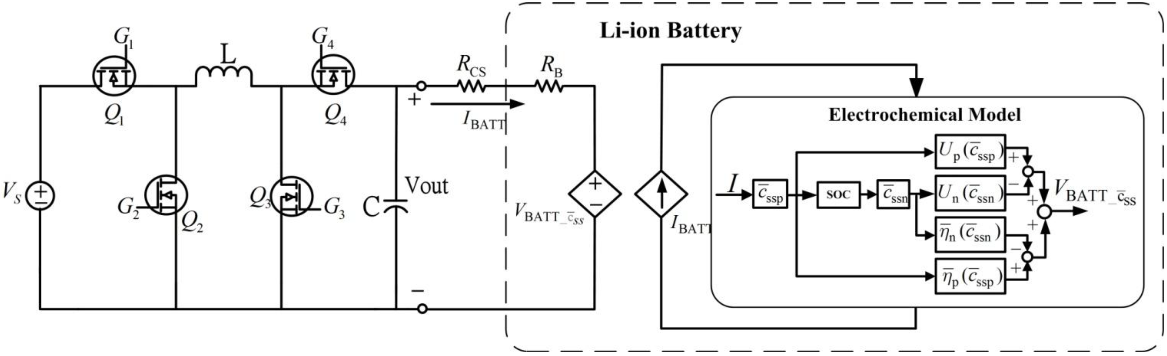
Figure 6 shows the circuit model for Li-ion battery charging with a buck-boost power converter which uses the electrochemical based equivalent circuit model from Section 2 (Figure 4) and the buck-boost converter from Section 3.

Figure 6. Equivalent circuit model for battery charging with buck-boost power converter.

Figure 6. Equivalent circuit model for battery charging with buck-boost power converter.

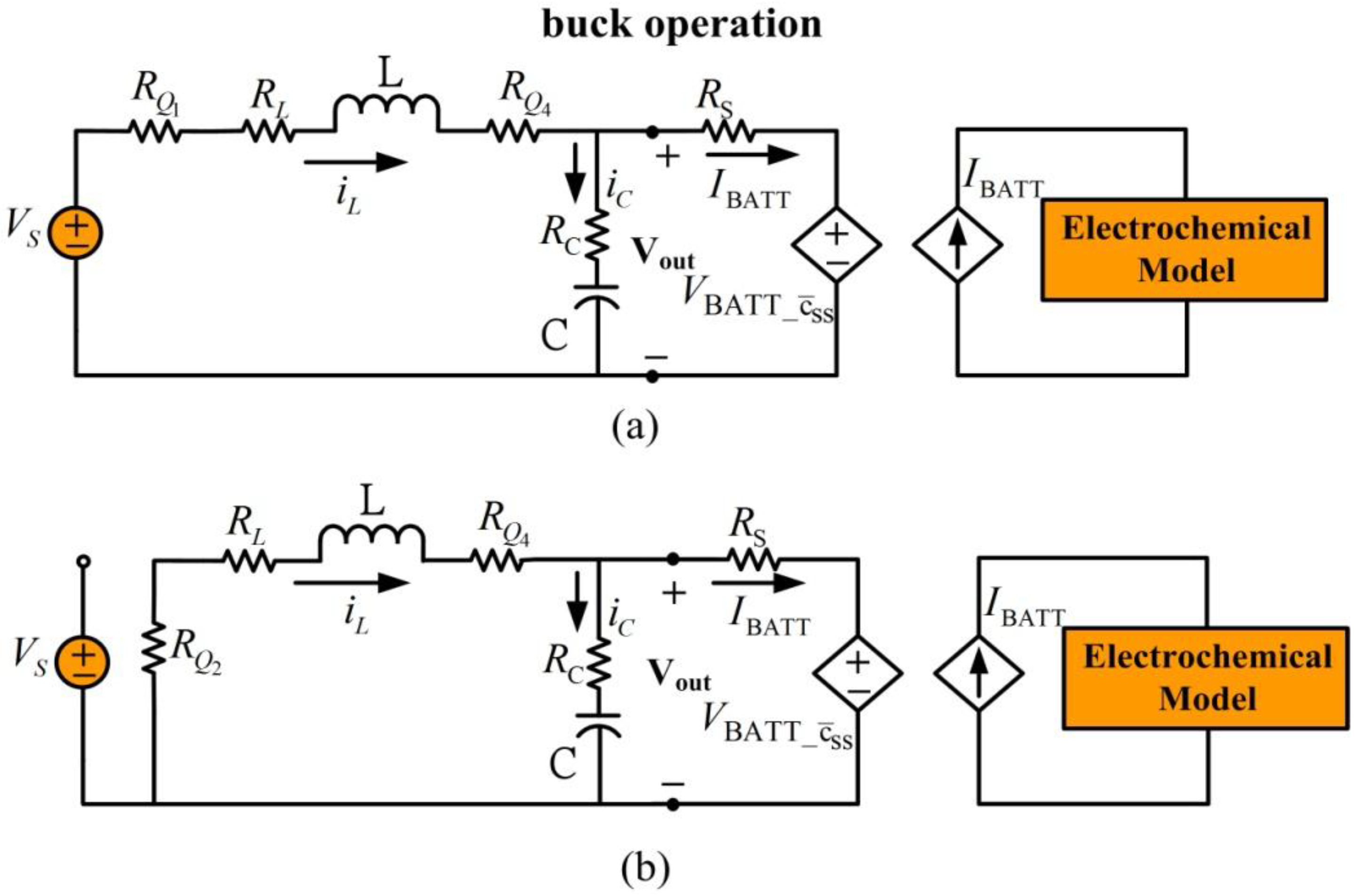
Resistance $R_{\text{CS}}$ is a current sense resistor, which is used by the battery charging controller to measure and control current to the battery. Figure 7 shows the equivalent circuit for battery charging in the buck model, which is similar to the buck-boost converter in Section 3.

Figure 7. Battery charging for buck mode operation. (a) Inductor charge, (b) inductor discharge.

Figure 7. Battery charging for buck mode operation. (a) Inductor charge, (b) inductor discharge.

The output regulation capacitor is modeled as an ideal capacitor with capacitance $C$ in series with its equivalent series resistance $R_C$. The inductor is modeled as an ideal inductor with inductance $L$ in series with its equivalent series resistance $R_L$. Resistor R_Qi represents the corresponding switch on resistance of the MOSFET. For simplicity, resistances $R_{CS}+R_B$ are replaced by a single resistor with resistance $R_S$. In this model, switch $Q_3$ is off and $Q_4$ is on. Buck operation is achieved by controlling switches $Q_1$ and $Q_2$ to charge and discharge the inductor and then transfer energy to the battery. Figure 7(a) shows the equivalent circuit for the inductor charging cycle and Figure 7(b) shows the inductor discharging equivalent circuit. If the duty cycle for inductor charging is $d$ and $d^{\prime }=1-d$ during inductor discharge, the averaged dynamic system for battery charging in buck mode operation is:

$$\begin{array}{c}\left[\begin{array}{c}\frac{d{i}_L}{dt}\\ \frac{d{v}_C}{dt}\end{array}\right]=\left[\begin{array}{cc}-\frac{(2R_Q+R_L)(R_C+R_S)+R_C{R}_S}{L(R_C+R_S)}& -\frac{R_S}{L(R_C+R_S)}\\ \frac{R_S}{C(R_C+R_S)}& -\frac{1}{C(R_C+R_S)}\end{array}\right]\left[\begin{array}{c}{i}_L\\ v_C\end{array}\right]+\left[\begin{array}{cc}\frac{d}{L}& -\frac{R_C}{L(R_C+R_S)}\\ 0& \frac{1}{C(R_C+R_S)}\end{array}\right]\left[\begin{array}{c}{V}_S\\ V_{{\text{BATT\_}\overline{\text{c}}}_{\text{ss}}}\end{array}\right]\\ \left[\begin{array}{c}{V}_{\text{out}}\\ I_{\text{BATT}}\end{array}\right]=\left[\begin{array}{cc}\frac{R_C{R}_S}{R_C+R_S}& \frac{R_S}{R_C+R_S}\\ \frac{R_C}{R_C+R_S}& \frac{1}{R_C+R_S}\end{array}\right]\left[\begin{array}{c}{i}_L\\ v_C\end{array}\right]+\left[\begin{array}{cc}0& \frac{R_C}{R_C+R_S}\\ 0& -\frac{1}{R_C+R_S}\end{array}\right]\left[\begin{array}{c}{V}_S\\ V_{{\text{BATT\_}\overline{\text{c}}}_{\text{ss}}}\end{array}\right]\end{array}$$

(35)

In this dynamic system, inductor current and capa citor voltage are system states. Inputs are external independent voltage source $V_S$ and dependent source $V_{{\text{BATT\_}\overline{\text{c}}}_{\text{ss}}}$ from the battery. System outputs are output terminal of the buck-boost converter $V_{\text{out}}$ and battery charging current $I_{\text{BATT}}$.

For simplicity, (35) assumes that switch-on resistances $R_{Q_1}=R_{Q_2}=R_{Q_3}=R_{Q_4}=R_Q$ because same part number are used for the power switches. One of the system inputs in (35) is dependent voltage source $V_{{\text{BATT\_}\overline{\text{c}}}_{\text{ss}}}$ from the battery. Voltage $V_{{\text{BATT\_}\overline{\text{c}}}_{\text{ss}}}$ is developed from the electrochemical model which is driven by an output from the battery charging model ($I_{\text{BATT}}$).The battery charging controller uses outputs $V_{\text{out}}$ and $I_{\text{BATT}}$ to determine the duty cycle for power switch operation. Therefore, battery charging forms a system with multiple interconnections, making system analysis and design more challenging and interesting. 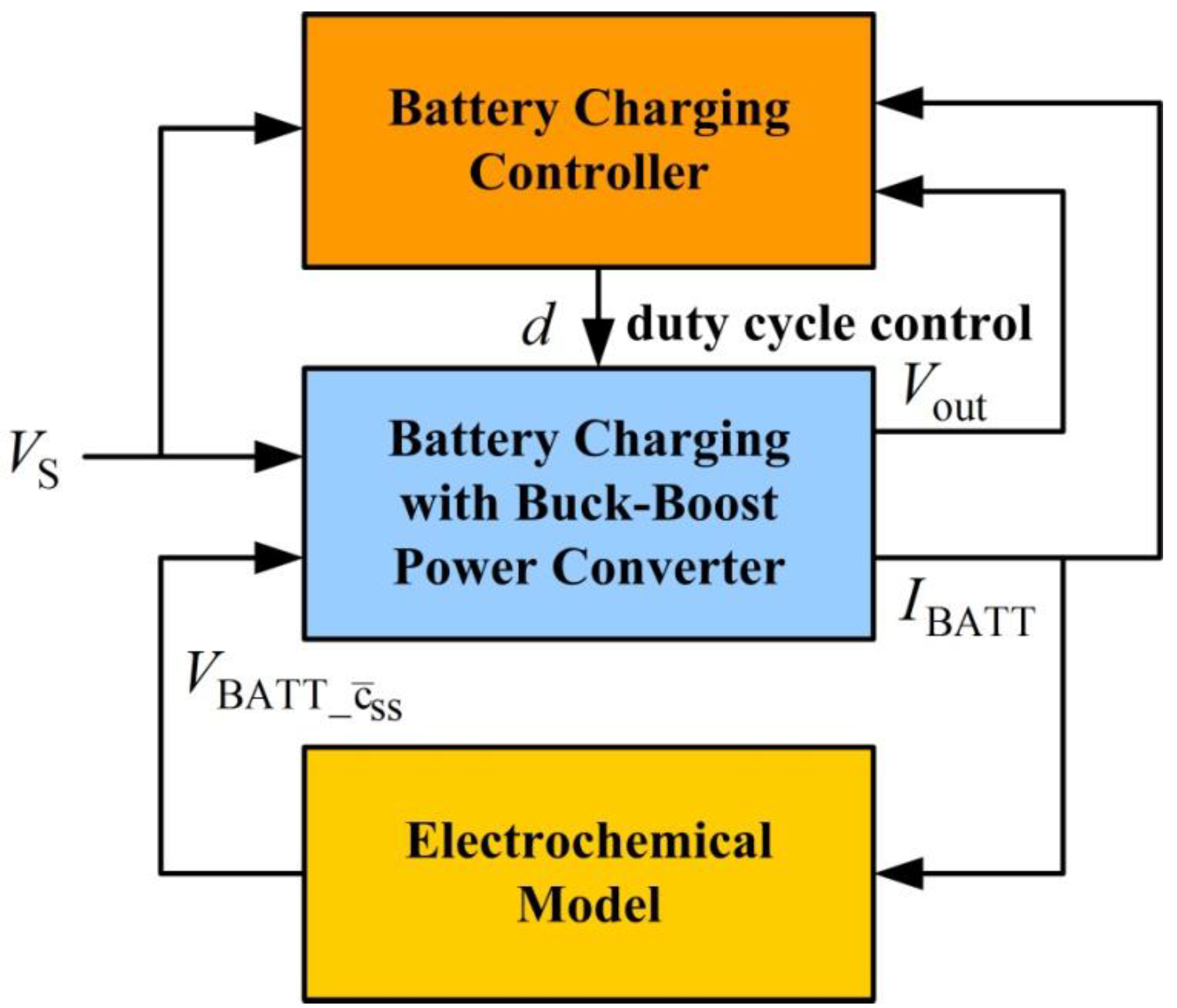Figure 8 shows the structure of the interconnected system.

Figure 8. System structure of the interconnected battery charging with buck-boost power converter.

Figure 8. System structure of the interconnected battery charging with buck-boost power converter.

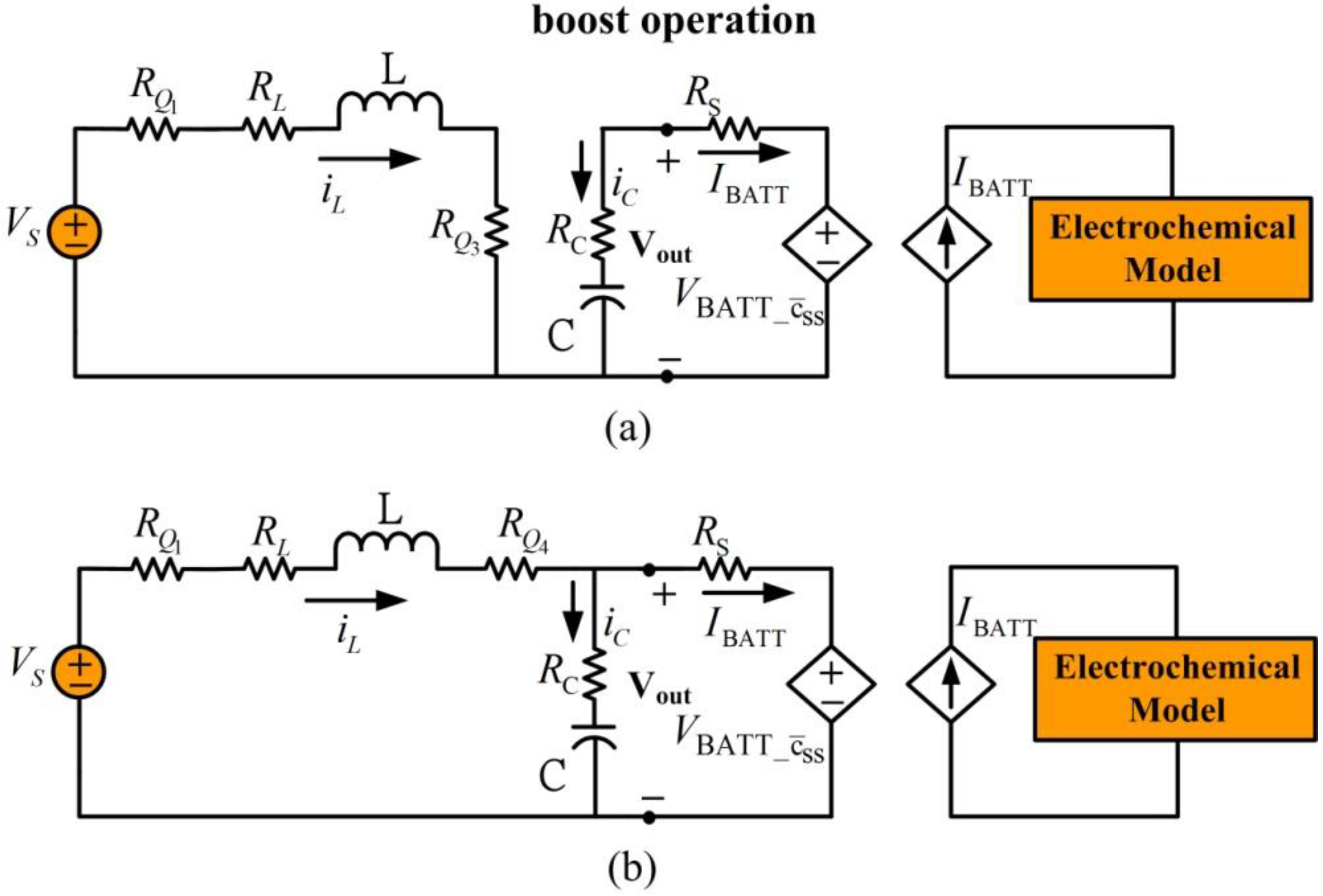
When external supplied voltage $V_S$ is less than the desired regulated output voltage, the converter is set to boost operation. In this mode, power switch $Q_1$ is on and $Q_2$ is off. Figure 9 shows the simplified equivalent circuits of battery charging during boost operation. In Figure 9(a), transistor $Q_3$ is closed and $Q_4$ is open, allowing the supply voltage to charge the inductor. In Figure 9(b), transistor $Q_4$ is closed and transistor $Q_3$ is open to engage inductor discharge mode. Similar to buck operation, the dynamic model for boost operation is expressed using the following equation:

$$\begin{array}{c}\left[\begin{array}{c}\frac{d{i}_L}{dt}\\ \frac{d{v}_C}{dt}\end{array}\right]=\left[\begin{array}{cc}-\frac{(2R_Q+R_L)(R_C+R_S)+d^{\prime }{R}_C{R}_S}{L(R_C+R_S)}& -\frac{d^{\prime }{R}_S}{L(R_C+R_S)}\\ \frac{d^{\prime }{R}_S}{C(R_C+R_S)}& -\frac{1}{C(R_C+R_S)}\end{array}\right]\left[\begin{array}{c}{i}_L\\ v_C\end{array}\right]+\left[\begin{array}{cc}\frac{1}{L}& -\frac{d^{\prime }{R}_C}{L(R_C+R_S)}\\ 0& \frac{1}{C(R_C+R_S)}\end{array}\right]\left[\begin{array}{c}{V}_S\\ V_{{\text{BATT\_}\overline{\text{c}}}_{\text{ss}}}\end{array}\right]\\ \left[\begin{array}{c}{V}_{\text{out}}\\ I_{\text{BATT}}\end{array}\right]=\left[\begin{array}{cc}\frac{d^{\prime }{R}_C{R}_S}{R_C+R_S}& \frac{R_S}{R_C+R_S}\\ \frac{d^{\prime }{R}_C}{R_C+R_S}& \frac{1}{R_C+R_S}\end{array}\right]\left[\begin{array}{c}{i}_L\\ v_C\end{array}\right]+\left[\begin{array}{cc}0& \frac{R_C}{R_C+R_S}\\ 0& -\frac{1}{R_C+R_S}\end{array}\right]\left[\begin{array}{c}{V}_S\\ V_{{\text{BATT\_}\overline{\text{c}}}_{\text{ss}}}\end{array}\right]\end{array}$$

(36)

Figure 9. Battery charging for boost mode operation. (a) Inductor charge, (b) inductor discharge.

Figure 9. Battery charging for boost mode operation. (a) Inductor charge, (b) inductor discharge.

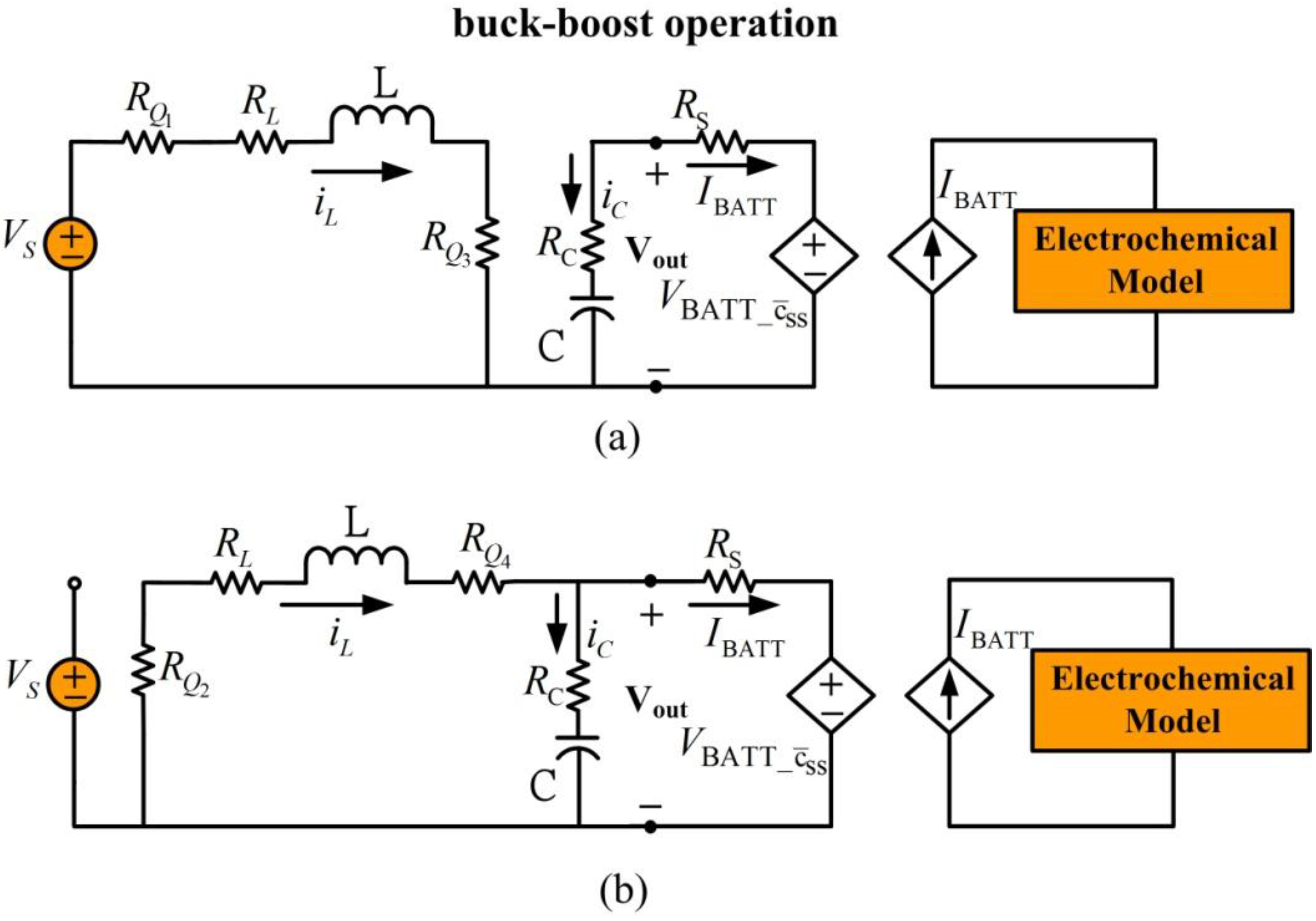
When supply voltage is close to the desired load voltage, the converter is set to buck-boost operation. Figure 10 shows the simplified equivalent circuits for battery charging during buck-boost operation. Transistors $Q_1$ and $Q_3$ work as a group and $Q_2$ and $Q_4$ work as another group.

Figure 10. Battery charging for buck-boost mode operation. (a) Inductor charge, (b) inductor discharge.

Figure 10. Battery charging for buck-boost mode operation. (a) Inductor charge, (b) inductor discharge.

In Figure 10(a), switches $Q_1$ and $Q_3$ are closed and $Q_2$ and $Q_4$ are open, allowing the supply voltage to charge the inductor. In Figure 10(b), transistors $Q_2$ and $Q_4$ are closed and transistors $Q_1$ and $Q_3$ are open to engage inductor discharge mode. During buck-boost operation, the inductor charge cycle is the same as the boost operation inductor charge cycle and the inductor discharge cycle is the same as the buck operation inductor discharge cycle. The averaged dynamic model for buck-boost operation is:

$$\begin{array}{c}\left[\begin{array}{c}\frac{d{i}_L}{dt}\\ \frac{d{v}_C}{dt}\end{array}\right]=\left[\begin{array}{cc}-\frac{(2R_Q+R_L)(R_C+R_S)+d^{\prime }{R}_C{R}_S}{L(R_C+R_S)}& -\frac{d^{\prime }{R}_S}{L(R_C+R_S)}\\ \frac{d^{\prime }{R}_S}{C(R_C+R_S)}& -\frac{1}{C(R_C+R_S)}\end{array}\right]\left[\begin{array}{c}{i}_L\\ v_C\end{array}\right]+\left[\begin{array}{cc}\frac{d}{L}& -\frac{d^{\prime }{R}_C}{L(R_C+R_S)}\\ 0& \frac{1}{C(R_C+R_S)}\end{array}\right]\left[\begin{array}{c}{V}_S\\ V_{{\text{BATT\_}\overline{\text{c}}}_{\text{ss}}}\end{array}\right]\\ \left[\begin{array}{c}{V}_{\text{out}}\\ I_{BATT}\end{array}\right]=\left[\begin{array}{cc}\frac{d^{\prime }{R}_C{R}_S}{R_C+R_S}& \frac{R_S}{R_C+R_S}\\ \frac{d^{\prime }{R}_C}{R_C+R_S}& \frac{1}{R_C+R_S}\end{array}\right]\left[\begin{array}{c}{i}_L\\ v_C\end{array}\right]+\left[\begin{array}{cc}0& \frac{R_C}{R_C+R_S}\\ 0& -\frac{1}{R_C+R_S}\end{array}\right]\left[\begin{array}{c}{V}_S\\ V_{{\text{BATT\_}\overline{\text{c}}}_{\text{ss}}}\end{array}\right]\end{array}$$

(37)

To investigate power converter performance for battery charging, this study conducts a stability analysis of duty cycle variation. Small signal models were obtained by applying a small disturbance to the system and ignoring second order terms. If the duty cycle with a small disturbance is $d=\overline{d}+\tilde{d}$ and $d^{\prime }={\overline{d}}^{\prime }-\tilde{d}$, the corresponding state and system output variations are $i_L={\overline{i}}_L+{\tilde{i}}_L$, $v_C={\overline{v}}_C+{\tilde{v}}_C$, $V_{\text{out}}={\overline{V}}_{\text{out}}+{\tilde{V}}_{\text{out}}$, and $I_{\text{BATT}}={\overline{I}}_{\text{BATT}}+{\tilde{I}}_{\text{BATT}}$. Variables $\overline{\phi }$ and $\tilde{\phi }$ represent the mean (or steady state) and variation of signal $\phi$. The small signal dynamic model driven by the small disturbance of duty cycle $\tilde{d}$ for buck mode operation is:

$$\begin{array}{c}\left[\begin{array}{c}\frac{d{\tilde{i}}_L}{dt}\\ \frac{d{\tilde{v}}_C}{dt}\end{array}\right]=\left[\begin{array}{cc}-\frac{(2R_Q+R_L)(R_C+R_S)+R_C{R}_S}{L(R_C+R_S)}& -\frac{R_S}{L(R_C+R_S)}\\ \frac{R_S}{C(R_C+R_S)}& -\frac{1}{C(R_C+R_S)}\end{array}\right]\left[\begin{array}{c}{\tilde{i}}_L\\ {\tilde{v}}_C\end{array}\right]+\left[\begin{array}{c}\frac{V_S}{L}\\ 0\end{array}\right]\tilde{d}\\ \left[\begin{array}{c}{\tilde{V}}_{\text{out}}\\ {\tilde{I}}_{\text{BATT}}\end{array}\right]=\left[\begin{array}{cc}\frac{R_C{R}_S}{R_C+R_S}& \frac{R_S}{R_C+R_S}\\ \frac{R_C}{R_C+R_S}& \frac{1}{R_C+R_S}\end{array}\right]\left[\begin{array}{c}{\tilde{i}}_L\\ {\tilde{v}}_C\end{array}\right]\end{array}$$

(38)

Equation (38) assumes that voltage sources $V_{\text{S}}$ and $V_{{\text{BATT\_}\overline{\text{c}}}_{\text{ss}}}$ remain constant when the system is disturbed by $\tilde{d}$ for a short period. Although dependent source $V_{{\text{BATT\_}\overline{\text{c}}}_{\text{ss}}}$ is driven by current $I_{\text{BATT}}$, its dynamics are much slower than the buck-boost converter circuit dynamics. This is easily verified by checking the Li-ion concentration diffusion dynamic bandwidth of the electrochemical model and the buck-boost power converter circuit dynamics. Input $V_{\text{S}}$ is an external voltage source. Therefore, these assumptions are reasonable.

Similarly, the small signal dynamic model driven by $\tilde{d}$ for boost mode operation is:

$$\begin{array}{c}\left[\begin{array}{c}\frac{d{\tilde{i}}_L}{dt}\\ \frac{d{\tilde{v}}_C}{dt}\end{array}\right]=\left[\begin{array}{cc}-\frac{(2R_Q+R_L)(R_C+R_S)+{\overline{d}}^{\prime }{R}_C{R}_S}{L(R_C+R_S)}& -\frac{{\overline{d}}^{\prime }{R}_S}{L(R_C+R_S)}\\ \frac{{\overline{d}}^{\prime }{R}_S}{C(R_C+R_S)}& -\frac{1}{C(R_C+R_S)}\end{array}\right]\left[\begin{array}{c}{\tilde{i}}_L\\ {\tilde{v}}_C\end{array}\right]\\ +\left[\begin{array}{c}\frac{R_C{R}_S{\overline{i}}_L+R_S{\overline{v}}_C+R_C{V}_{{\text{BATT\_}\overline{\text{c}}}_{\text{ss}}}}{L(R_C+R_S)}\\ -\frac{R_S{\overline{i}}_L}{C(R_C+R_S)}\end{array}\right]\tilde{d}\\ \left[\begin{array}{c}{\tilde{V}}_{\text{out}}\\ {\tilde{I}}_{\text{BATT}}\end{array}\right]=\left[\begin{array}{cc}\frac{{\overline{d}}^{\prime }{R}_C{R}_S}{R_C+R_S}& \frac{R_S}{R_C+R_S}\\ \frac{{\overline{d}}^{\prime }{R}_C}{R_C+R_S}& \frac{1}{R_C+R_S}\end{array}\right]\left[\begin{array}{c}{\tilde{i}}_L\\ {\tilde{v}}_C\end{array}\right]+\left[\begin{array}{c}-\frac{R_C{R}_S{\overline{i}}_L}{R_C+R_S}\\ -\frac{R_C{\overline{i}}_L}{R_C+R_S}\end{array}\right]\tilde{d}\end{array}$$

(39)

Similarly, the small signal dynamic model for buck-boost mode operation is:

$$\begin{array}{c}\left[\begin{array}{c}\frac{d{\tilde{i}}_L}{dt}\\ \frac{d{\tilde{v}}_C}{dt}\end{array}\right]=\left[\begin{array}{cc}-\frac{(2R_Q+R_L)(R_C+R_S)+{\overline{d}}^{\prime }{R}_C{R}_S}{L(R_C+R_S)}& -\frac{{\overline{d}}^{\prime }{R}_S}{L(R_C+R_S)}\\ \frac{{\overline{d}}^{\prime }{R}_S}{C(R_C+R_S)}& -\frac{1}{C(R_C+R_S)}\end{array}\right]\left[\begin{array}{c}{\tilde{i}}_L\\ {\tilde{v}}_C\end{array}\right]\\ +\left[\begin{array}{c}\frac{R_C{R}_S{\overline{i}}_L+R_S{\overline{v}}_C+(R_C+R_S)V_S+R_C{V}_{{\text{BATT\_}\overline{\text{c}}}_{\text{ss}}}}{L(R_C+R_S)}\\ -\frac{R_S{\overline{i}}_L}{C(R_C+R_S)}\end{array}\right]\tilde{d}\\ \left[\begin{array}{c}{\tilde{V}}_{\text{out}}\\ {\tilde{I}}_{\text{BATT}}\end{array}\right]=\left[\begin{array}{cc}\frac{{\overline{d}}^{\prime }{R}_C{R}_S}{R_C+R_S}& \frac{R_S}{R_C+R_S}\\ \frac{{\overline{d}}^{\prime }{R}_C}{R_C+R_S}& \frac{1}{R_C+R_S}\end{array}\right]\left[\begin{array}{c}{\tilde{i}}_L\\ {\tilde{v}}_C\end{array}\right]+\left[\begin{array}{c}-\frac{R_C{R}_S{\overline{i}}_L}{R_C+R_S}\\ -\frac{R_C{\overline{i}}_L}{R_C+R_S}\end{array}\right]\tilde{d}\end{array}$$

(40)

Equations (38) to (40) show that ${\tilde{V}}_{\text{out}}=R_S{\tilde{I}}_{\text{BATT}}$. Therefore, only characteristics of dynamics from $\tilde{d}$ to ${\tilde{V}}_{\text{out}}$ are investigated.

System characteristics depend on inductance $L$ and capacitance $C$. Factors which must be considered to determine inductance include input voltage range, output voltage, inductor current, and switching frequency for duty cycle control. The capacitor maintains well-regulated voltage and capacitance depends on the inductor current ripple, switching frequency, and the desired output voltage ripple. In this design, input voltage varies from 8 to 30 V. Output is designed to charge the Li-ion battery. The battery consists of three Li-ion battery cells connected in series. Battery voltage is approximately 12.6 V when fully charged. This study uses inductance L = 4.7 mH and capacitance C = 396 mF. System characteristics also depend on operating conditions (such as battery voltage $V_{\text{BATT}}$, inductor current $i_L$, and capacitor voltage $v_{\text{C}}$), equivalent series resistances $R_L$ and $R_C$, and MOSFET on resistance $R_Q$. For good voltage regulation with low output voltage ripples and minimal power loss from inherent inductor resistance, components with low $R_C$, $R_L$, and $R_Q$ values for the capacitor, inductor, and power MOSFETs, respectively, are used in the power converter design.

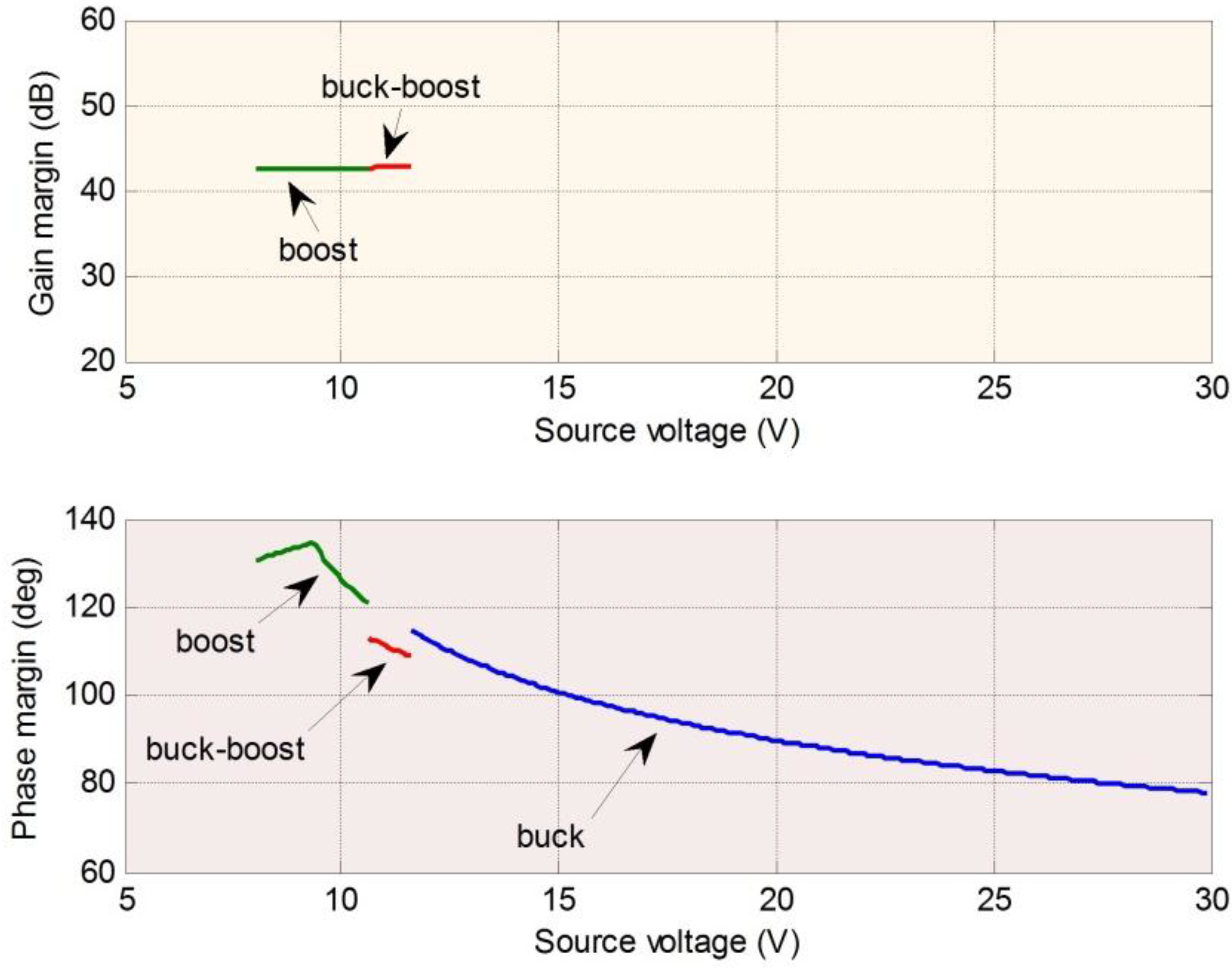
Assuming 300-kHz switching frequency, 3-A charge current, 11-V battery, R_L = 50 mW, R_C = 5 mW and R_O = 7 mW, Figure 11 shows the stability margins of the system from duty cycle variation $\tilde{d}$ to output voltage variation ${\tilde{V}}_{\text{out}}$ with respect to supply voltage variation. The figure indicates that the phase margins are inadequate.

Figure 11. Stability margin of the buck-boost power converter.

Figure 11. Stability margin of the buck-boost power converter.

DC/DC power converter design commonly incorporates a type III compensator into the system to improve the phase margin. The type III compensator, as shown in Figure 12, uses six passive circuit components, three poles (one at the origin), and two zeros. The compensator transfer function is:

$$K(s)=-\frac{\left(R_2{C}_{2}s+1\right)\left[\left(R_1+R_3\right)C_{3}s+1\right]}{R_1\left(C_1+C_2\right)s\left(R_2{C}_{12}s+1\right)\left(R_3{C}_{3}s+1\right)},$$

(41)

where $C_{12}$ is the parallel combination of $C_1$ and $C_2$, that is, $C_{12}=C_1{C}_2/(C_1+C_2)$. Figure 13 shows the power converter stability margins with incorporated compensator when R₁ = 10 kW, R₂ = 668 W, R₃ = 630 W, C₁ = 1.05 nF, C₂ = 161 nF and C₃ = 10.1 nF. Table 2 shows a summary of stability margins. The results show that the phase margins improve significantly. The results for 1-A and 0.1-A charge current are also investigated. The stability margin will be improved when the load current decreases. 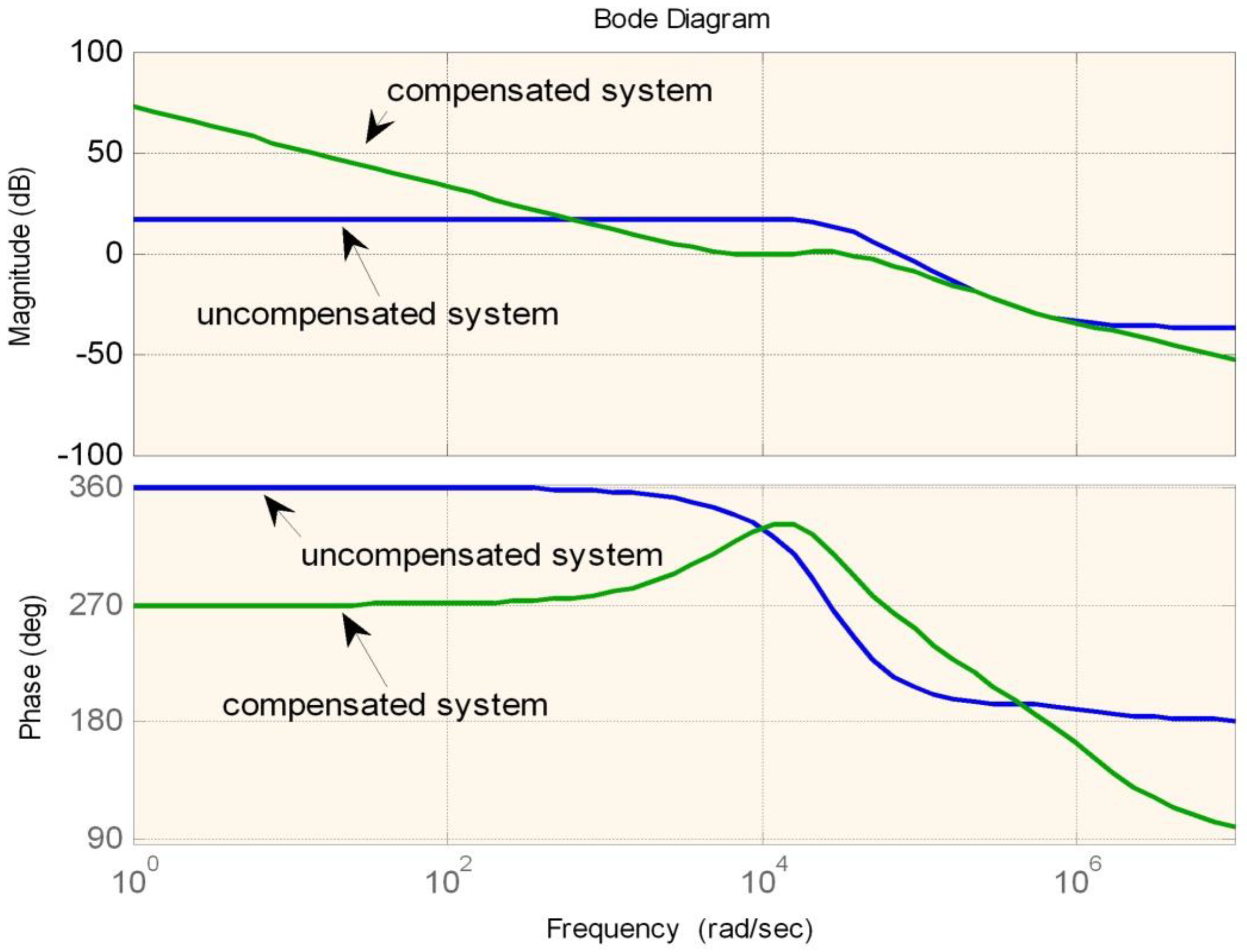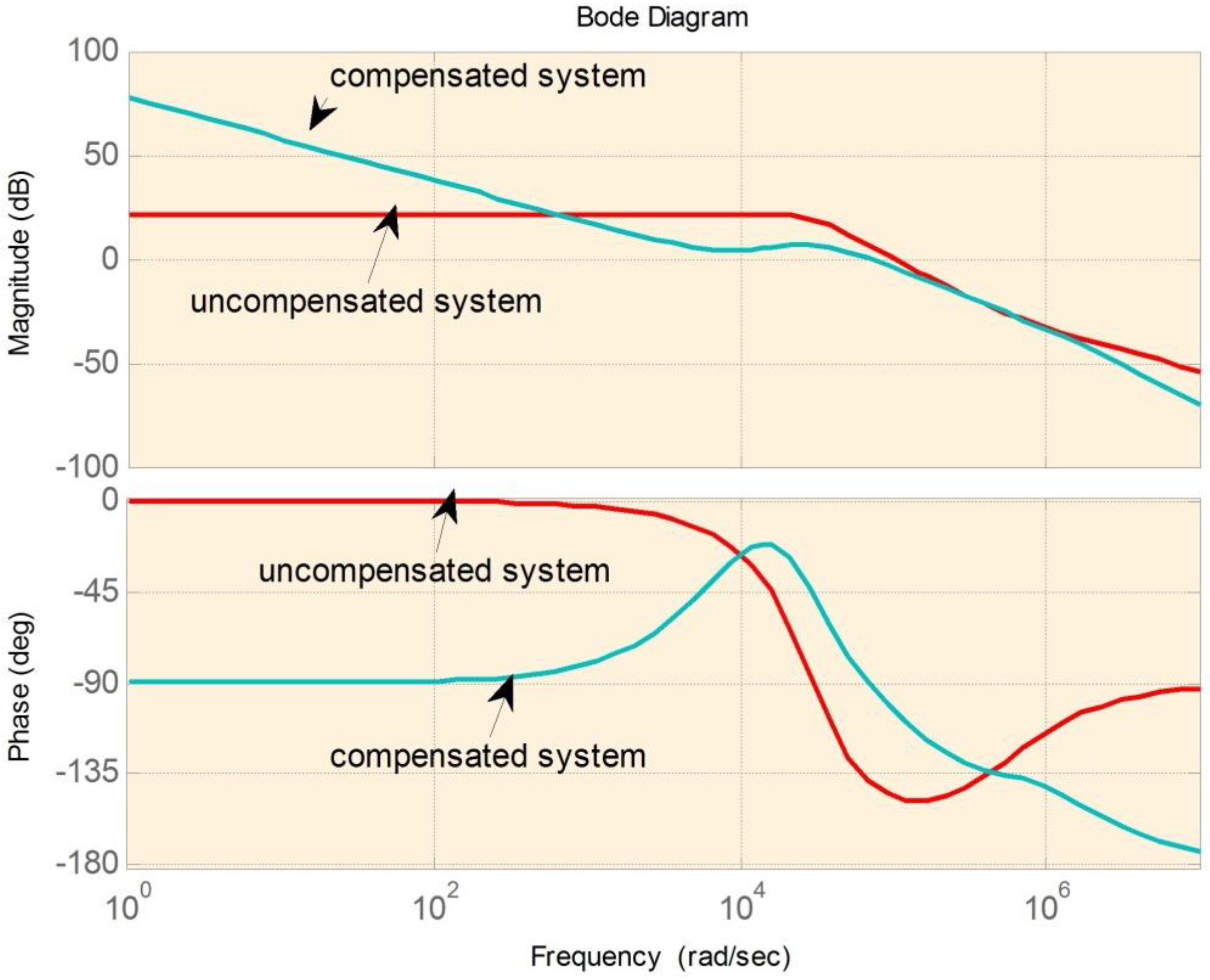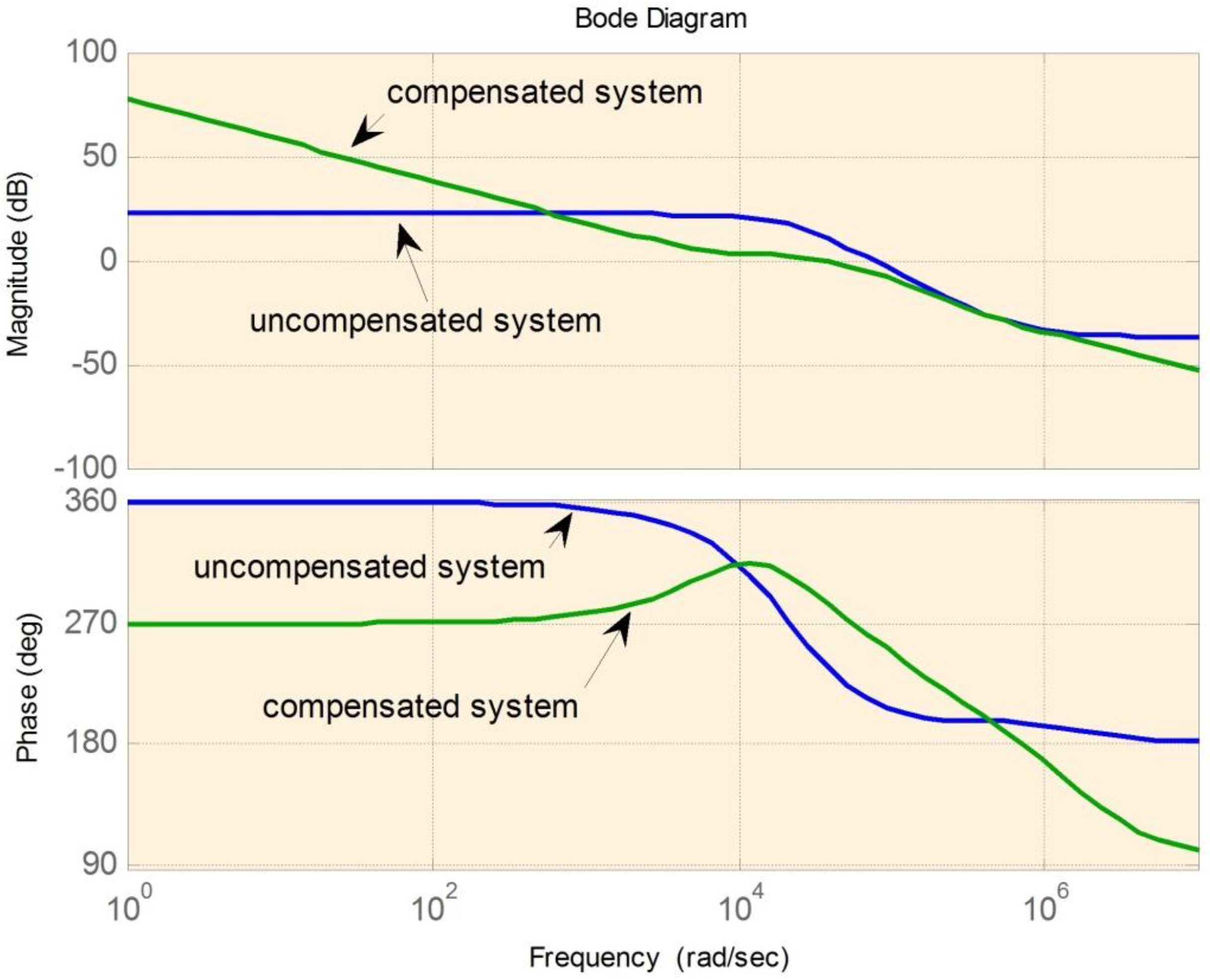Figure 14, Figure 15 and Figure 16 are the examples of the bode plots for boost, buck-boost, and buck modes respectively. The bode plots examples clearly show the improvement of the phase margin for the compensated system.

Figure 12. The type III compensator.

Figure 12. The type III compensator.

Figure 13. Stability of the power converter with type III controller incorporated.

Figure 13. Stability of the power converter with type III controller incorporated.

Figure 14. Bode plot for boost mode.

Figure 14. Bode plot for boost mode.

Figure 15. Bode plot for buck-boost mode.

Figure 15. Bode plot for buck-boost mode.

Figure 16. Bode plot for buck mode.

Figure 16. Bode plot for buck mode.

Table 2. Summary of the stability margins of the power converter.

Mode	Stability margin	Without compensator	With compensator
Buck mode $11.8 \text{V}<V_{\text{S}}\le 30 \text{V}$	Gain margin (dB)	$\infty$	$\infty$
	Phase margin (deg)	31.77–38.22	78.05–113.65
Buck-Boost mode $10.8 \text{V}<V_{\text{S}}\le 11.8 \text{V}$	Gain margin (dB)	36.89	31.77–31.95
	Phase margin (deg)	31.65–32.35	106.82–111.27
Boost mode $8 \text{V}<V_{\text{S}}\le 10.8 \text{V}$	Gain margin (dB)	36.89	31.06–31.77
	Phase margin (deg)	33.70–36.27	118.65–134.11

Table 2. Summary of the stability margins of the power converter.

Mode	Stability margin	Without compensator	With compensator
Buck mode $11.8 \text{V}<V_{\text{S}}\le 30 \text{V}$	Gain margin (dB)	$\infty$	$\infty$
	Phase margin (deg)	31.77–38.22	78.05–113.65
Buck-Boost mode $10.8 \text{V}<V_{\text{S}}\le 11.8 \text{V}$	Gain margin (dB)	36.89	31.77–31.95
	Phase margin (deg)	31.65–32.35	106.82–111.27
Boost mode $8 \text{V}<V_{\text{S}}\le 10.8 \text{V}$	Gain margin (dB)	36.89	31.06–31.77
	Phase margin (deg)	33.70–36.27	118.65–134.11

These results show that stability margins depend on the selected inductor and capacitor and the load condition. The system switches between the three operation modes according to the supply voltage condition. Supply voltage variation arises from rapid changes in atmosphere conditions or sunlight incident angle changes. Therefore, as well as stability considerations for each individual operation mode, the mean square stability of the jump system must be considered.

The system switches between buck, buck-boost, and boost operation modes according to supply voltage conditions. Considering the worst case scenario (based on stability margins), the state space models for the three modes are expressed as:

$$\{\begin{array}{c}\dot{x}=A_{i}x+B_{i}u\\ y=C_{i}x+D_{i}u\end{array} i=1,2,3,$$

(42)

where $x={\left[\begin{array}{cc}{\tilde{i}}_L& {\tilde{v}}_C\end{array}\right]}^T$, $u=\tilde{d}$, $y={\tilde{V}}_{\text{out}}$, and $i=1$ represent buck mode, $i=2$ represents buck-boost mode, and $i=3$ represents boost mode. The system matrices for $L=4.7 \mu \text{H}$ and $C=396 \mu \text{F}$ with 3-A loads are as follows:

Buck mode:

$$\begin{array}{l}{A}_1=\left[\begin{array}{cc}-1.463\times {10}^4& -2.028\times {10}^5\\ 2407& -2.361\times {10}^4\end{array}\right] , B_1=\left[\begin{array}{c}6.363\times {10}^6\\ 0\end{array}\right]\\ C_1=\left[\begin{array}{cc}0.004766& 0.9533\end{array}\right] , D_1=0\end{array}$$

(43)

Buck-boost mode:

$$\begin{array}{l}{A}_2=\left[\begin{array}{cc}-1.414\times {10}^4& -1.036\times {10}^5\\ 1230& -2.361\times {10}^4\end{array}\right], B_2=\left[\begin{array}{c}4.917\times {10}^6\\ -7222\end{array}\right]\\ C_2=\left[\begin{array}{cc}0.002435& 0.9533\end{array}\right] , D_2=-0.0143\end{array}$$

(44)

Boost mode:

$$\begin{array}{l}{A}_3=\left[\begin{array}{cc}-1.459\times {10}^4& -1.937\times {10}^5\\ 2299& -2.361\times {10}^4\end{array}\right] , B_3=\left[\begin{array}{c}2.406\times {10}^6\\ -7222\end{array}\right]\\ C_3=\left[\begin{array}{cc}0.004533& 0.9533\end{array}\right] , D_3=-0.0143\end{array}$$

(45)

For mean square stability analysis of the power converter system, we convert the system to discrete time domain and model the system as a Markov jump linear system [32] with three operation modes as:

$$G:\hspace{1em}\{\begin{array}{c}x[k+1]=A_{\theta [k]}x[k]+B_{\theta [k]}u[k]\\ y[k]=C_{\theta [k]}x[k]+D_{\theta [k]}u[k]\\ x[0]=x_0,\hspace{0.17em}\theta [0]={\theta }_0\end{array}$$

(46)

where $\theta [k]\in \left\{1,2,3\right\}$ is a stationary Markov chain and system parameters $A_{\theta [k]}, B_{\theta [k]}, C_{\theta [k]},$ and $D_{\theta [k]}$ change with $\theta [k]$. The probability of transition between all modes is described using matrix $P={\left[p_{ij}\right]}_{3\times 3}$, $i,j\in \left\{1,2,3\right\}$ , $p_{ij}\ge 0$, and $\forall i, {\displaystyle {\sum }_{j=1}^3{p}_{ij}}=1$. The Markov jump system in (46) is mean square stable if and only if a collection of positive definite matrices ($X_1, X_2, X_3$) exist such that the following linear matrix inequality (LMI) is satisfied [32]:

$$\forall i\in \left\{1,2,3\right\}, A_i^T\left({\displaystyle {\sum }_{j=1}^3{p}_{ij}{X}_j}\right)A_i-X_i<0$$

(47)

.

Figure 17 shows the Markov jump system and its mean square stability conditions.

Figure 17. Markov Jump Linear System with three Operation Modes.

Figure 17. Markov Jump Linear System with three Operation Modes.

Using the switching frequency of the power converter, 300 kHz, as the sampling rate to convert the systems represented in (43) to (45), the system matrices in the discrete time domain are:

Buck mode:

$$\begin{array}{l}{A}_1=\left[\begin{array}{cc}0.9496& -0.6337\\ 0.007737& 0.9217\end{array}\right] , B_1=\left[\begin{array}{c}20.68\\ 0.08386\end{array}\right]\\ C_1=\left[\begin{array}{cc}0.004766& 0.9533\end{array}\right] , D_1=0\end{array}$$

(48)

Buck-boost mode:

$$\begin{array}{l}{A}_2=\left[\begin{array}{cc}0.9533& -0.3242\\ 0.003849& 0.9237\end{array}\right], B_2=\left[\begin{array}{c}16.01\\ 0.009075\end{array}\right]\\ C_2=\left[\begin{array}{cc}0.002435& 0.9533\end{array}\right], D_2=-0.0143\end{array}$$

(49)

Boost mode:

$$\begin{array}{l}{A}_3=\left[\begin{array}{cc}0.9502& -0.6054\\ 0.007185& 0.9220\end{array}\right], B_3=\left[\begin{array}{c}7.829\\ 0.006313\end{array}\right]\\ C_3=\left[\begin{array}{cc}0.004533& 0.9533\end{array}\right] , D_3=-0.0143\end{array}$$

(50)

The mean square stability condition described in (47) can be verified using the MATLAB LMI toolbox. For example, assuming the following probability transition matrix P is selected:

$$P=\left[\begin{array}{ccc}0.9& 0.1& 0\\ 0.2& 0.6& 0.2\\ 0& 0.3& 0.7\end{array}\right],$$

(51)

The resulting positive definite matrices are:

$$X_1=\left[\begin{array}{cc}17.915& -27.0367\\ -27.0367& 514.7221\end{array}\right], X_2=\left[\begin{array}{cc}28.5660& -15.3102\\ -15.3102& 520.2183\end{array}\right], X_3=\left[\begin{array}{cc}34.6270& -22.1413\\ -22.1413& 568.5330\end{array}\right]$$

(52)

This implies that the jump systems are mean square stable for the selected probability transition matrix. However, the buck-boost converter system stability margins depend on the system parameters (such as inductor and capacitor values, battery voltage, and battery charging current). The system shall be designed to provide good stability margins for each individual operation mode and to guarantee the mean square stability of the jump system. It should be noted that the analysis made here is valid for continuous conduction modes only.

5. Electric Circuit Simulation

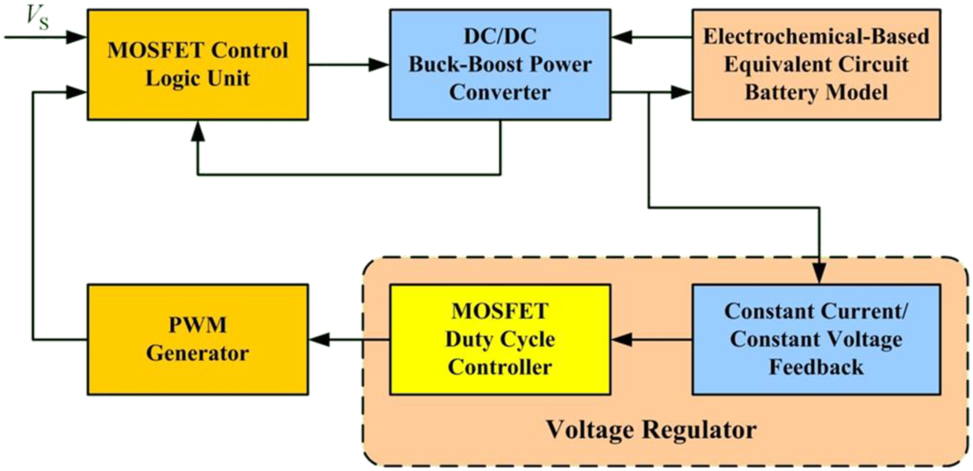
The battery charging model developed in the previous sections was used in a computer simulation using the MATLAB-based PLECS tool to verify the buck-boost converter design for Li-ion battery charging. Figure 18 shows the simulation structure. The structure includes a MOSFET control logic unit, a buck-boost power converter, an electrochemical-based equivalent circuit model, a voltage regulator, and a PWM generator.

Figure 18. The block diagram of the PLECS computer simulation.

Figure 18. The block diagram of the PLECS computer simulation.

The MOSFET control logic unit determines the power converter operating mode. In this simulation, buck mode was engaged (set to logic 1) if source voltage $V_{\text{S}}$ was greater than or equal to output voltage $V_{\text{out}}$ plus threshold $V_{\text{T}}$, that is, $V_{\text{S}}\ge V_{\text{out}}+V_{\text{T}}$. If not, buck mode was set to logic 0. 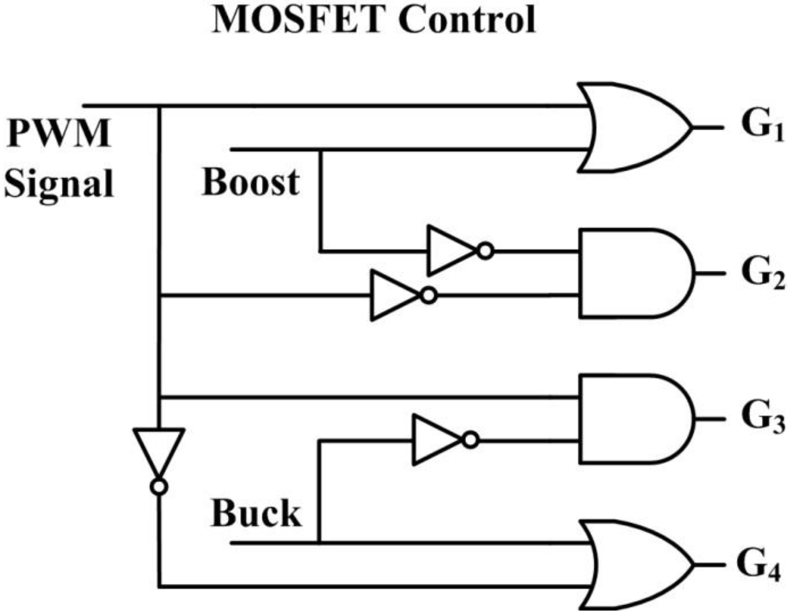If $V_{\text{S}}\le V_{\text{out}}-V_{\text{T}}$, boost mode was set to logic 1 and set to logic 0 if not. Buck-boost mode was set to logic 1 if both buck and boost modes were set to logic 0. These definitions were used to establish the structure of the MOSFET control logic unit, as shown in Figure 19. Outputs $G_1~G_4$ in Figure 19 are the control gates of power switches $Q_1~Q_4$ shown in Figure 6. We note that in practical use, hysteresis or some other means of switch controls to ensure continuous mode transition has to be incorporated to minimize possible large transient during mode transition.

Figure 19. Logic circuit for the MOSFET control.

Figure 19. Logic circuit for the MOSFET control.

The buck-boost converter and electrochemical-based equivalent circuit battery model discussed in the previous sections were directly used in the simulation. Electrochemical model parameters from [27] were used, except for utilization ratios θ_p and θ_n (θ_p0% = 0.895, θ_p100% = 0.305, θ_n0% = 0.126 and θ_n100% = 0.676 were selected). Table 3 lists the parameters used in the simulation. Constant current or constant voltage feedback determined the battery charging mode. The duty cycle controller determined the proper duty ratio for the power switches. In this simulation, $d=\overline{d}+\tilde{d}$ determined the duty ratio and the type III compensator described in the previous section determined variation $\tilde{d}$. Mean value $\overline{d}$ was defined using the following equations:

$$\overline{d}=\frac{{\overline{V}}_{\text{out}}}{V_{\text{S}}}\cdot \text{Buck}+\frac{{\overline{V}}_{\text{out}}-V_{\text{S}}}{{\overline{V}}_{\text{out}}}\cdot \text{Boost}+\frac{{\overline{V}}_{\text{out}}}{{\overline{V}}_{\text{out}}+V_{\text{S}}}\cdot \left(\overline{\text{Buck}+\text{Boost}}\right)$$

(53)

for constant voltage charging mode and:

$$\begin{array}{c}\overline{d}=\frac{{\overline{I}}_{\text{BATT}}\cdot R_{\text{S}}+V_{{\text{BATT\_}\overline{\text{c}}}_{\text{ss}}}}{V_{\text{S}}}\cdot \text{Buck}+\frac{{\overline{I}}_{\text{BATT}}\cdot R_{\text{S}}+V_{{\text{BATT\_}\overline{\text{c}}}_{\text{ss}}}-V_{\text{S}}}{{\overline{I}}_{\text{BATT}}\cdot R_{\text{S}}+V_{{\text{BATT\_}\overline{\text{c}}}_{\text{ss}}}}\cdot \text{Boost}\\ +\frac{{\overline{I}}_{\text{BATT}}\cdot R_{\text{S}}+V_{{\text{BATT\_}\overline{\text{c}}}_{\text{ss}}}}{{\overline{I}}_{\text{BATT}}\cdot R_{\text{S}}+V_{{\text{BATT\_}\overline{\text{c}}}_{\text{ss}}}+V_{\text{S}}}\cdot \left(\overline{\text{Buck}+\text{Boost}}\right)\end{array}$$

(54)

for constant current charging mode. Variables Buck and Boost in (53) and (54) are Boolean signals and ${\overline{V}}_{\text{out}}$ and ${\overline{I}}_{\text{BATT}}$ are desired regulated voltage and current, respectively. Equations (53) and (54) are formulated using Equations (35) to (37) by setting $d{i}_L/dt=0$ and $d{v}_C/dt=0$ and assuming that R_L = 0, R_C = 0 and R_Q = 0.

Table 3. Battery Parameters.

Parameter	Negative electrode	Separator	Positive electrode
Thickness, $L^{-}, L^{\text{sep}}, L^{+}$ (cm)	50 × 10−4	25.4 × 10−4	36.4 × 10−4
Particle radius, $R_{\text{s}}$ (cm)	1 × 10−4	-	1 × 10−4
Active material volume fraction, ${\epsilon }_{\text{s}}$	0.580	-	0.500
Electrolyte phase volume fraction, ${\epsilon }_{\text{e}}$	0.332	0.5	0.330
Solid phase conductivity, $\sigma ({\text{Ω}}^{-1}{\text{cm}}^{-1})$	1.0	-	0.1
${\text{Li}}^{+}$ Transference number, $t_{+}^0$	0.363
Electrolyte phase ionic conductivity, $\kappa ({\text{Ω}}^{-1}{\text{cm}}^{-1})$	$\kappa =15.8c_{\text{e}}\text{exp}[0.85{(1000c_{\text{e}})}^{1.4}$
Electrolyte phase diffusion coefficient, $D_{\text{e}} ({\text{cm}}^2{\text{s}}^{-1})$	2.6 × 10−6
Solid phase diffusion coefficient, $D_{\text{s}}({\text{cm}}^2{\text{s}}^{-1})$	2.0 × 10−12	-	3.7 × 10−12
Maximum solid phase concentration, $c_{\text{s},\text{max}} (\text{mol}\cdot {\text{cm}}^{-3})$	16.1 × 10−3	-	23.9 × 10−3
Exchange current density, $i_0 (\text{A}\cdot {\text{cm}}^2)$	3.6 × 10−3		2.6 × 10−3
Average electrolyte concentration, ${\overline{c}}_{\text{e}} (\text{mol}\cdot {\text{cm}}^{-3})$	1.2 × 10−3
Charge-transfer coefficients, ${\alpha }_a,{\alpha }_c$	0.5, 0.5	-	0.5, 0.5
Active surface area per electrode unit volume, $a ({\text{cm}}^{-1})$	$a_{\text{s,n}}=3{\epsilon }_{\text{e}}/R_{\text{s}}$	-	$a_{\text{s,n}}=3{\epsilon }_{\text{e}}/R_{\text{s}}$
Utilization ratio at 0% SOC, ${\theta }_{\text{n}0\%},{\theta }_{\text{p}0\%}$	0.126	-	0.895
Utilization ratio at 100% SOC, ${\theta }_{\text{n}100\%},{\theta }_{\text{p}100\%}$	0.676	-	0.305
Electrode plate area, A $({\text{cm}}^2)$	10452	-	10452
Current collector contact resistance, $R_{\text{f}} (\text{Ω}{\text{cm}}^2)$	20
Equilibrium potential, Negative electrode	$\begin{array}{c}{U}_{\text{n}}({\theta }_{\text{n}})=8.0029+5.0647{\theta }_{\text{n}}-12.578{\theta }_{\text{n}}^{0.5}\\ -8.6322\times {10}^{-4}{\theta }_{\text{n}}^{-1}+2.176\times {10}^{-5}{\theta }_{\text{n}}^{3/2}\\ -0.46016\text{exp}[15.0(0.06-{\theta }_{\text{n}}]\\ -0.55364\text{exp}[-2.4326({\theta }_{\text{n}}-0.92)]\end{array}$
Equilibrium potential, Positive electrode	$\begin{array}{c}{U}_{\text{p}}({\theta }_{\text{p}})=85.681{\theta }_{\text{p}}^6-357.70{\theta }_{\text{p}}^5+613.89{\theta }_{\text{p}}^4\\ -555.65{\theta }_{\text{p}}^3+281.06{\theta }_{\text{p}}^2-76.648{\theta }_{\text{p}}\\ +13.1983-0.30987\text{exp}(5.657{\theta }_{\text{p}}^{115})\end{array}$

Table 3. Battery Parameters.

Parameter	Negative electrode	Separator	Positive electrode
Thickness, $L^{-}, L^{\text{sep}}, L^{+}$ (cm)	50 × 10−4	25.4 × 10−4	36.4 × 10−4
Particle radius, $R_{\text{s}}$ (cm)	1 × 10−4	-	1 × 10−4
Active material volume fraction, ${\epsilon }_{\text{s}}$	0.580	-	0.500
Electrolyte phase volume fraction, ${\epsilon }_{\text{e}}$	0.332	0.5	0.330
Solid phase conductivity, $\sigma ({\text{Ω}}^{-1}{\text{cm}}^{-1})$	1.0	-	0.1
${\text{Li}}^{+}$ Transference number, $t_{+}^0$	0.363
Electrolyte phase ionic conductivity, $\kappa ({\text{Ω}}^{-1}{\text{cm}}^{-1})$	$\kappa =15.8c_{\text{e}}\text{exp}[0.85{(1000c_{\text{e}})}^{1.4}$
Electrolyte phase diffusion coefficient, $D_{\text{e}} ({\text{cm}}^2{\text{s}}^{-1})$	2.6 × 10−6
Solid phase diffusion coefficient, $D_{\text{s}}({\text{cm}}^2{\text{s}}^{-1})$	2.0 × 10−12	-	3.7 × 10−12
Maximum solid phase concentration, $c_{\text{s},\text{max}} (\text{mol}\cdot {\text{cm}}^{-3})$	16.1 × 10−3	-	23.9 × 10−3
Exchange current density, $i_0 (\text{A}\cdot {\text{cm}}^2)$	3.6 × 10−3		2.6 × 10−3
Average electrolyte concentration, ${\overline{c}}_{\text{e}} (\text{mol}\cdot {\text{cm}}^{-3})$	1.2 × 10−3
Charge-transfer coefficients, ${\alpha }_a,{\alpha }_c$	0.5, 0.5	-	0.5, 0.5
Active surface area per electrode unit volume, $a ({\text{cm}}^{-1})$	$a_{\text{s,n}}=3{\epsilon }_{\text{e}}/R_{\text{s}}$	-	$a_{\text{s,n}}=3{\epsilon }_{\text{e}}/R_{\text{s}}$
Utilization ratio at 0% SOC, ${\theta }_{\text{n}0\%},{\theta }_{\text{p}0\%}$	0.126	-	0.895
Utilization ratio at 100% SOC, ${\theta }_{\text{n}100\%},{\theta }_{\text{p}100\%}$	0.676	-	0.305
Electrode plate area, A $({\text{cm}}^2)$	10452	-	10452
Current collector contact resistance, $R_{\text{f}} (\text{Ω}{\text{cm}}^2)$	20
Equilibrium potential, Negative electrode	$\begin{array}{c}{U}_{\text{n}}({\theta }_{\text{n}})=8.0029+5.0647{\theta }_{\text{n}}-12.578{\theta }_{\text{n}}^{0.5}\\ -8.6322\times {10}^{-4}{\theta }_{\text{n}}^{-1}+2.176\times {10}^{-5}{\theta }_{\text{n}}^{3/2}\\ -0.46016\text{exp}[15.0(0.06-{\theta }_{\text{n}}]\\ -0.55364\text{exp}[-2.4326({\theta }_{\text{n}}-0.92)]\end{array}$
Equilibrium potential, Positive electrode	$\begin{array}{c}{U}_{\text{p}}({\theta }_{\text{p}})=85.681{\theta }_{\text{p}}^6-357.70{\theta }_{\text{p}}^5+613.89{\theta }_{\text{p}}^4\\ -555.65{\theta }_{\text{p}}^3+281.06{\theta }_{\text{p}}^2-76.648{\theta }_{\text{p}}\\ +13.1983-0.30987\text{exp}(5.657{\theta }_{\text{p}}^{115})\end{array}$

In the simulation, the battery was charged with a constant current until battery voltage reached the maximal voltage limit. The circuit then switched to constant voltage mode, allowing the current to taper. The battery module consisted of three Li-ion battery cells connected in series. Before simulating the complete charging process, constant current and constant voltage charging were conducted for a short period to verify battery charging performance using the buck-boost converter. 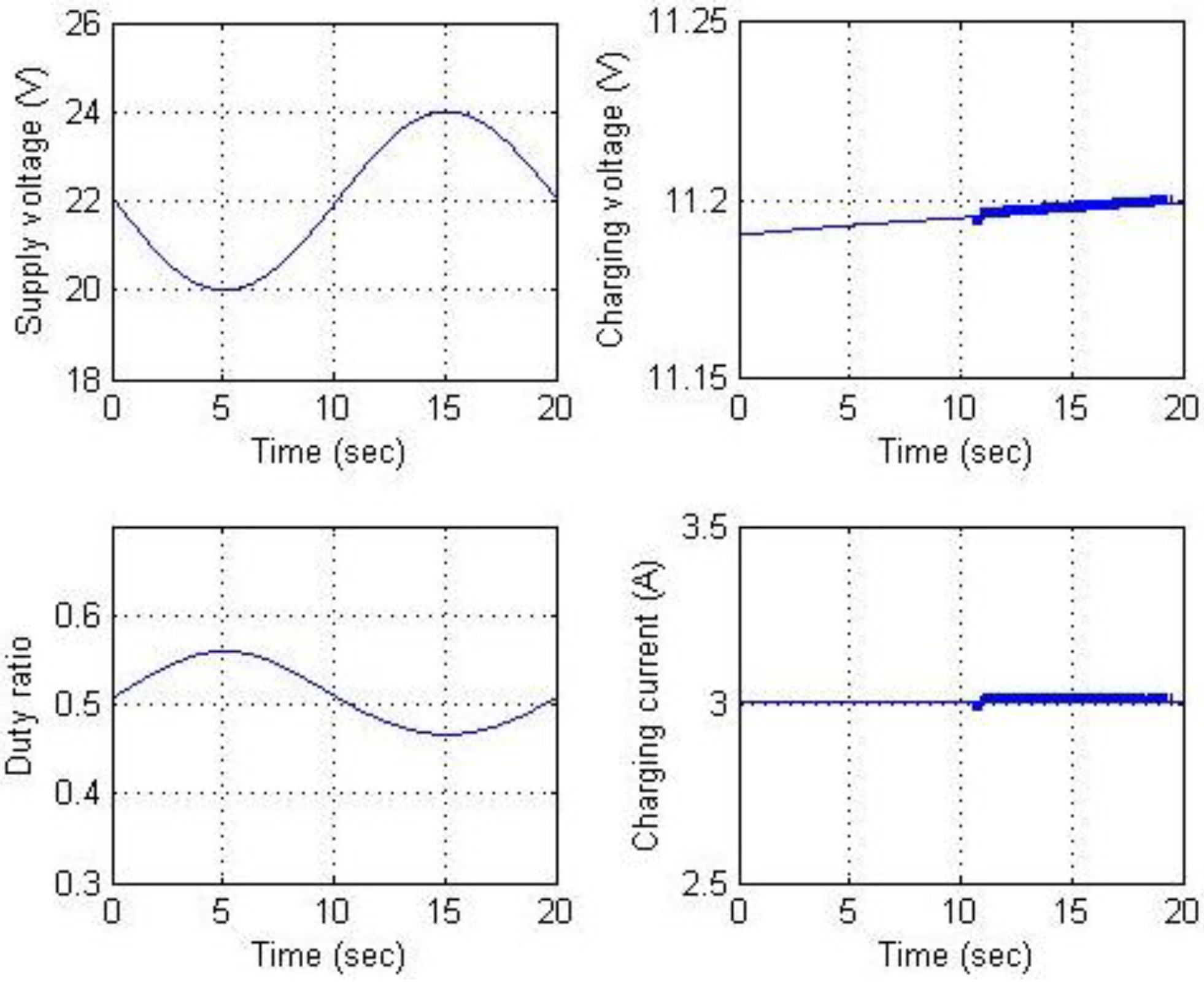Figure 20 and Figure 21 show the simulation results for constant current charging. The goal of the circuit simulation was to maintain a battery charging current of 3 A while the supply voltage varied from 20 to 24 V. This supply voltage was selected because the voltage output of the maximal power point of the solar power panels used was approximately 22 V. The supply voltage, charging voltage, power switch duty ratio, and charging current are shown in Figure 20. The results show that the charging current is regulated at 3 A as expected. 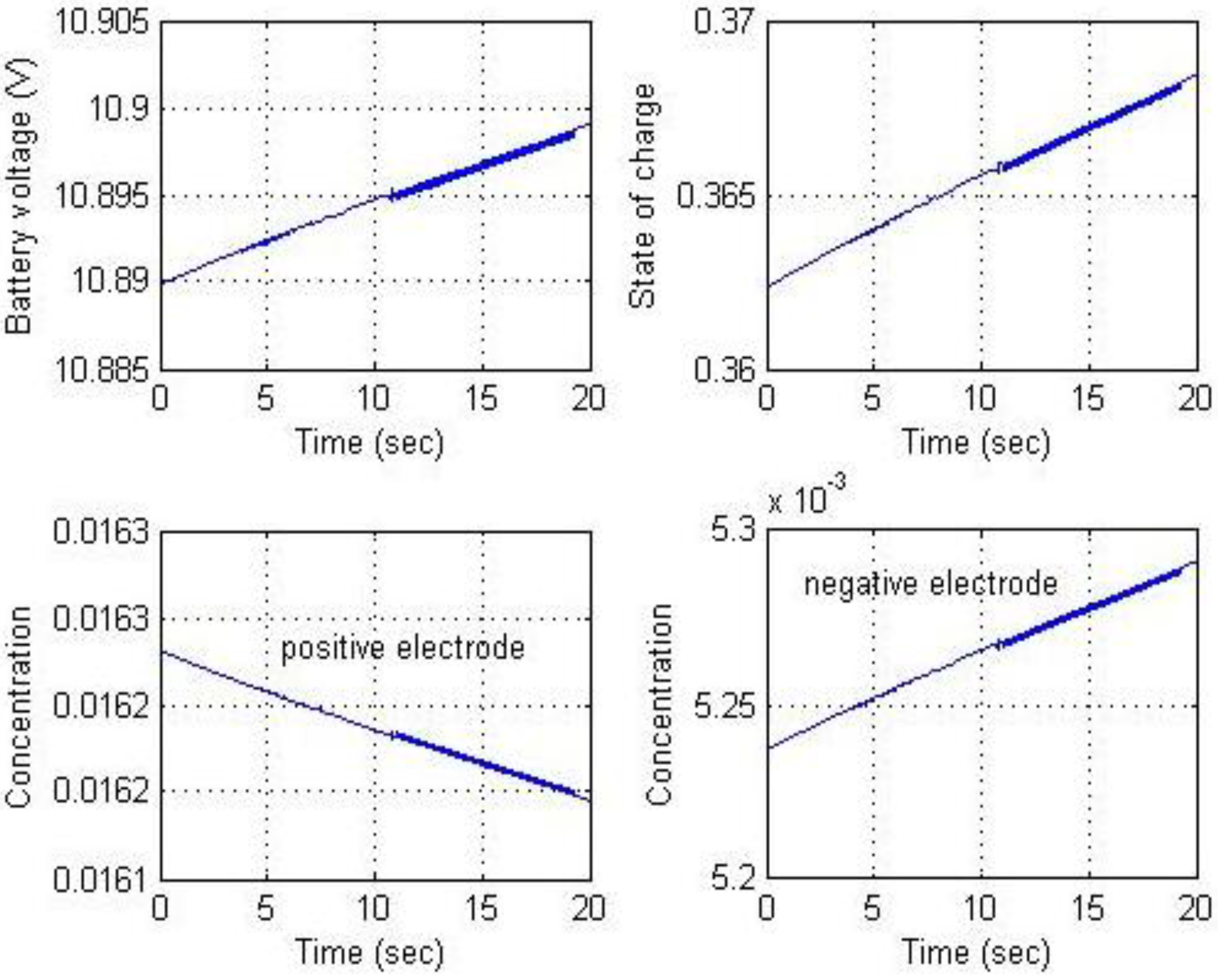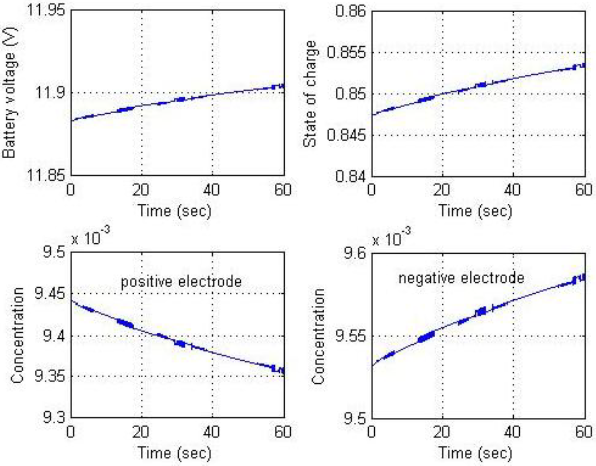Figure 21 shows the results for battery voltage, SOC, and Li-ion solid concentrations for the positive and negative electrodes. 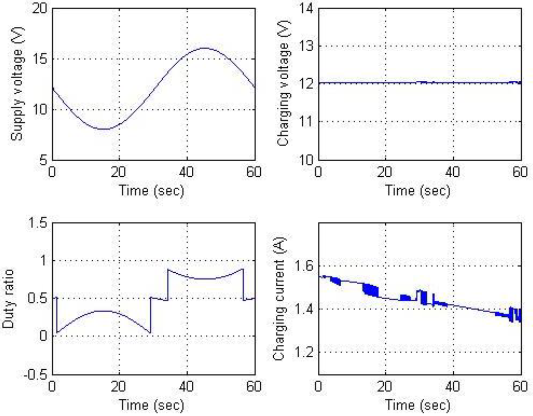Figure 22 and Figure 23 show the results for constant voltage charging. Supply voltage varied from 8 to 16 V to ensure that mode transition occurred during the simulation. Maintaining a charging voltage of 12 V was the simulation goal. 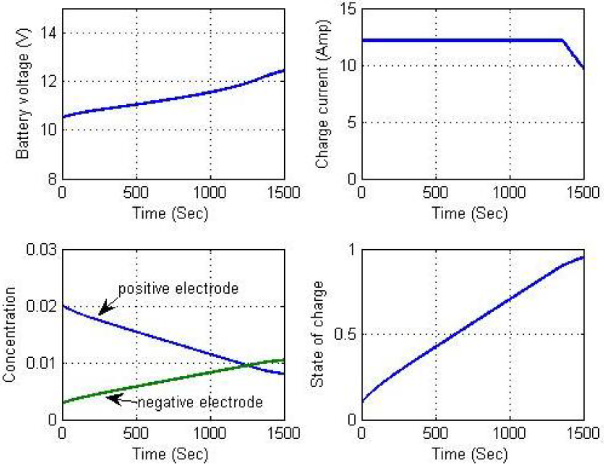Figure 22 indicates that the charging voltage was regulated at 12 V. Because the constant current and constant voltage charging simulations were successful, long-term continuous charging began with constant current charging followed by constant voltage to demonstrate the complete charging process. To accelerate the simulation, a charging current of 12 A was used for the constant current phase. The charging process switched to constant voltage charging mode when battery voltage reached 12.6 V. These results are shown in Figure 24. They include battery voltage, charging current, Li-ion solid concentrations, and SOC computations. The chattering phenomena appear in Figure 20 and Figure 21 are due to the nonlinear behavior of the electrochemical-based battery model, and those in Figure 22 and Figure 23 are from the combination of nonlinear behavior of the battery model and mode transition because hysteresis is not included in the simulation.

The circuit simulations show that the battery was successfully charged with the buck-boost power converter. Battery parameters such as battery voltage, Li-ion solid concentrations, and SOC were calculated based-on the electrochemical model. Thus, the buck-boost power converter can be used for battery charging in solar powered battery management systems.

Figure 20. Results for constant current charging (a).

Figure 20. Results for constant current charging (a).

Figure 21. Results for constant current charging (b).

Figure 21. Results for constant current charging (b).

Figure 22. Results for constant voltage charging (a).

Figure 22. Results for constant voltage charging (a).

Figure 23. Results for constant voltage charging (b).

Figure 23. Results for constant voltage charging (b).

Figure 24. Results for long-term battery charging.

Figure 24. Results for long-term battery charging.

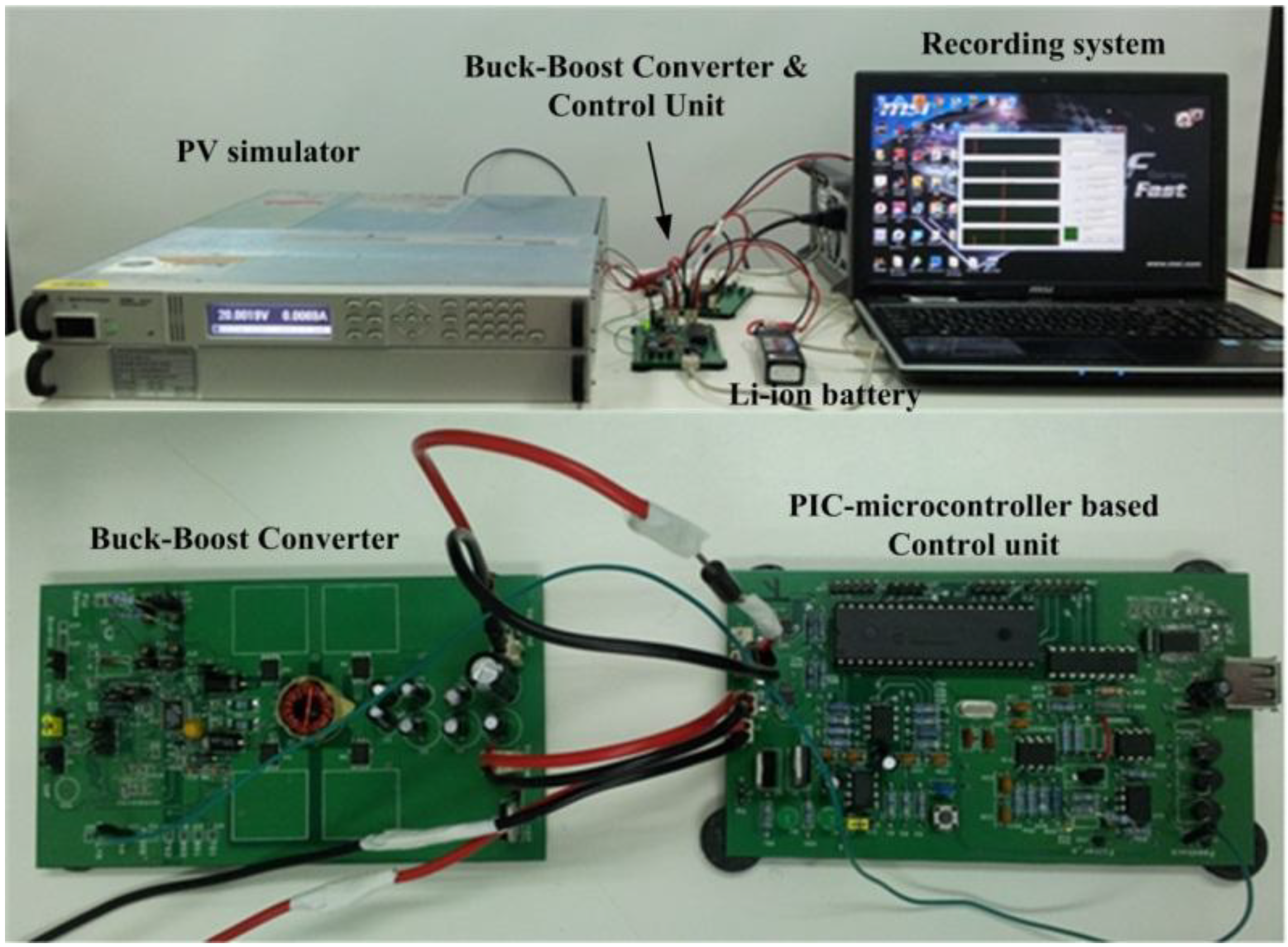
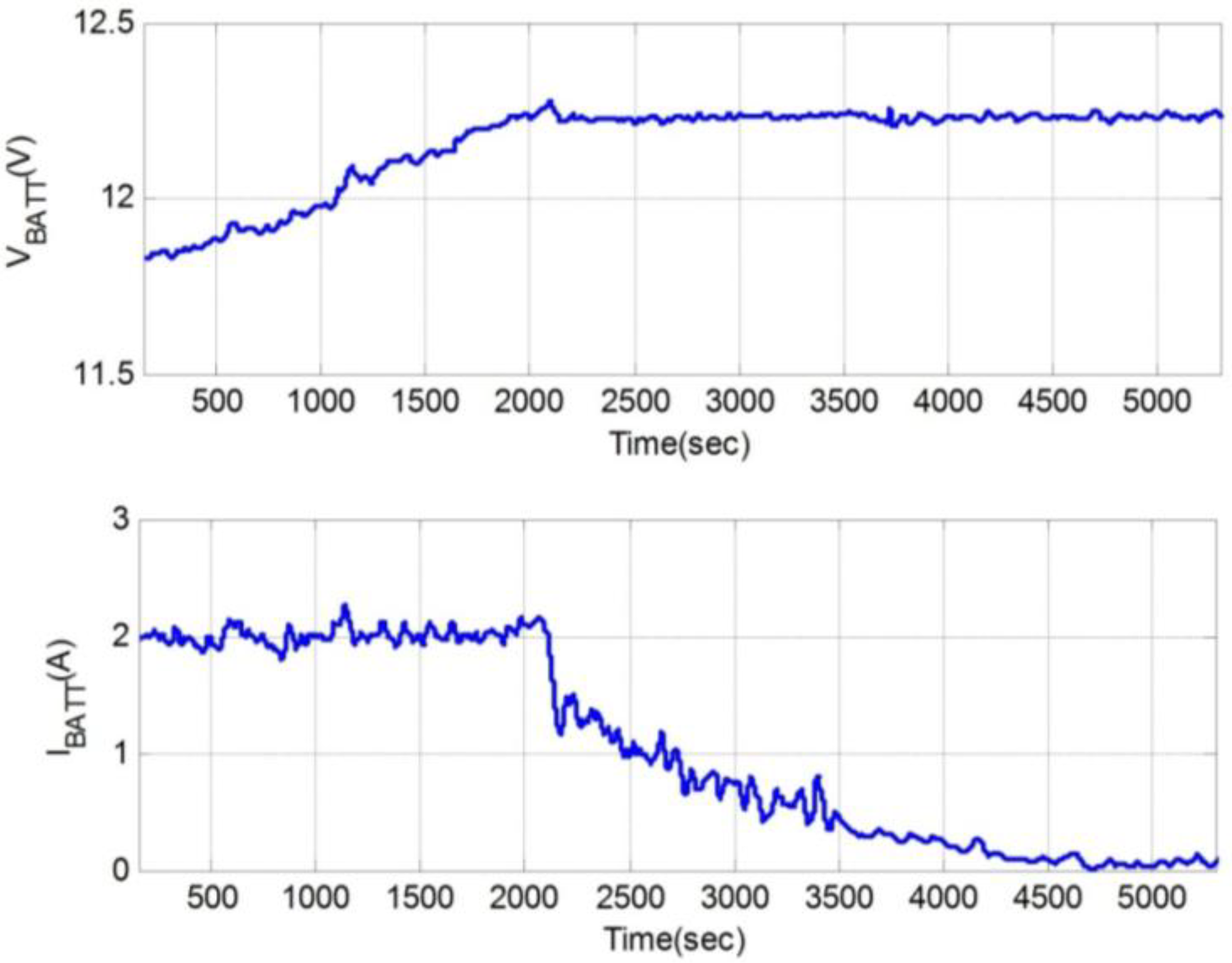
To demonstrate the battery charging design using a buck-boost power converter, a prototype of the battery charging system is built to conduct battery charging tests. To accelerate the design, we selected a LTC3780 four-switch type buck-boost controller (from Linear Technology Corporation, Milpitas, CA, USA) to control the MOSFET switches. A PIC-microcontroller based control unit is then designed to perform the battery charging mechanism. Images of the test set-up, buck-boost converter, and the control unit are shown in Figure 25. In this test, the power source comes from the photovoltaic simulator (PV simulator) and the results are transmitted to the recording system over USB interface. The battery is charged by a constant current of 2A until the battery voltage reaches 12.3 V. The system then switches to constant voltage charging mode, allowing the battery current to taper. Test results are shown in Figure 26. The results show the success of Li-ion battery charging using buck-boost converter based battery charging system.

Figure 25. Test set-up for battery charging (top) and buck-boost converter & control unit (bottom).

Figure 25. Test set-up for battery charging (top) and buck-boost converter & control unit (bottom).

Figure 26. Results of battery charging using buck-boost converter based battery charging system.

Figure 26. Results of battery charging using buck-boost converter based battery charging system.

7. Conclusions

This paper presents an analysis and simulation of the Li-ion battery charging process for a solar powered battery management system. Based on the supply voltage conditions of solar panels, the system operates in buck, buck-boost, or boost modes. Based on an electrode averaged electrochemical model, an equivalent circuit model is established to represent Li-ion battery dynamics. The battery model and buck-boost power converter dynamic models are used to construct a mathematical model describing the battery charging process dynamics. The battery charging process forms a system with several interconnections. Characteristics including battery charging system stability margins for each individual operating mode are analyzed and discussed. The system is also modeled as a Markov jump system to evaluate the mean square stability of the system. A MATLAB-based Simulink PLECS tool verifies the battery charging model.

With the success of battery charging analysis and circuit simulation the synchronous buck-boost converter will be used for the design of a solar power management system for an experimental solar-powered UAV, including the maximum power point tracking and battery management applications. The proposed electrochemical-based equivalent circuit model will be used to estimate the battery dynamics. The core of the solar power management system will be the buck-boost converter with microcontroller based auto-ranging capability. In addition, we will also investigate SEPIC and zeta buck-boost converters in the next design.