Banki-Michell Optimal Design by Computational Fluid Dynamics Testing and Hydrodynamic Analysis

 ,
,  and
and
Abstract
:1. Introduction
2. The State of the Art on Michell-Banki Parameter Design


| Design parameters | values | Description of the design parameters |
|---|---|---|
| D2/D1 | 0.68 | Diameter Ratio |
| α | 22° | Angle of attack |
| β2 | 90° | Blade exit angle |
| λ | 90° | Inlet discharge angle |
| Nb | 35 | Number of blades |
3. The Proposed Two-Step Design Procedure
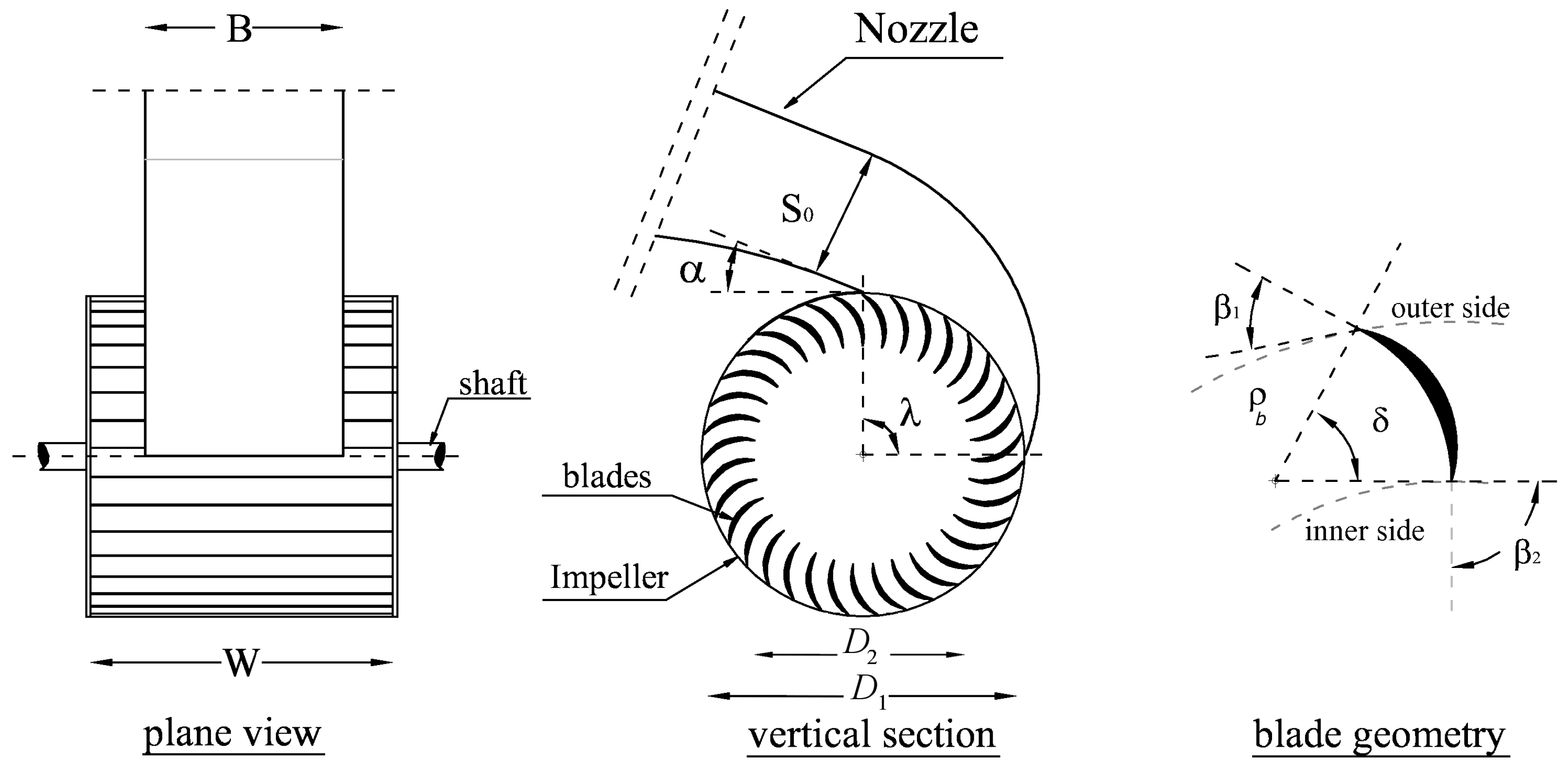
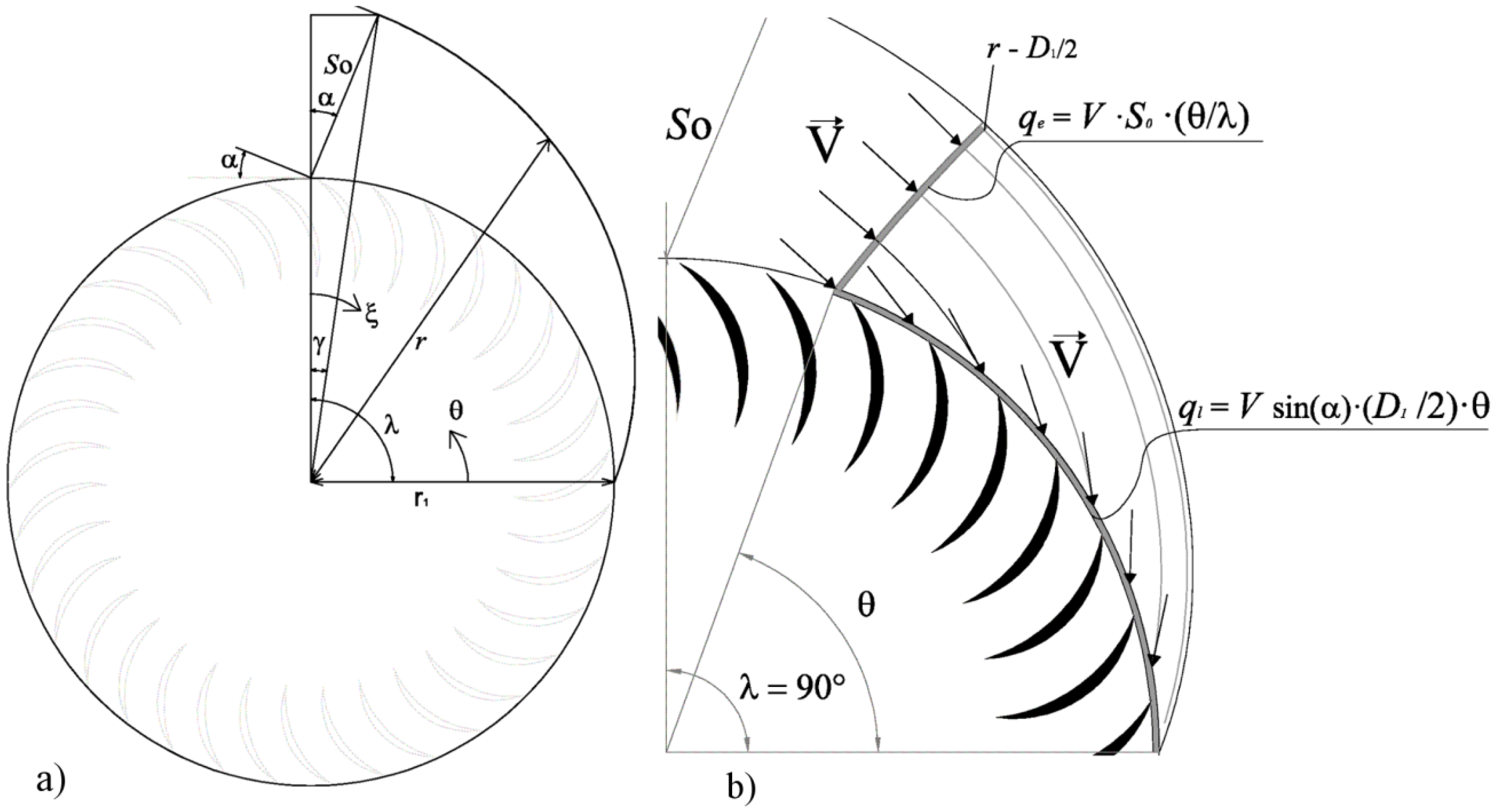
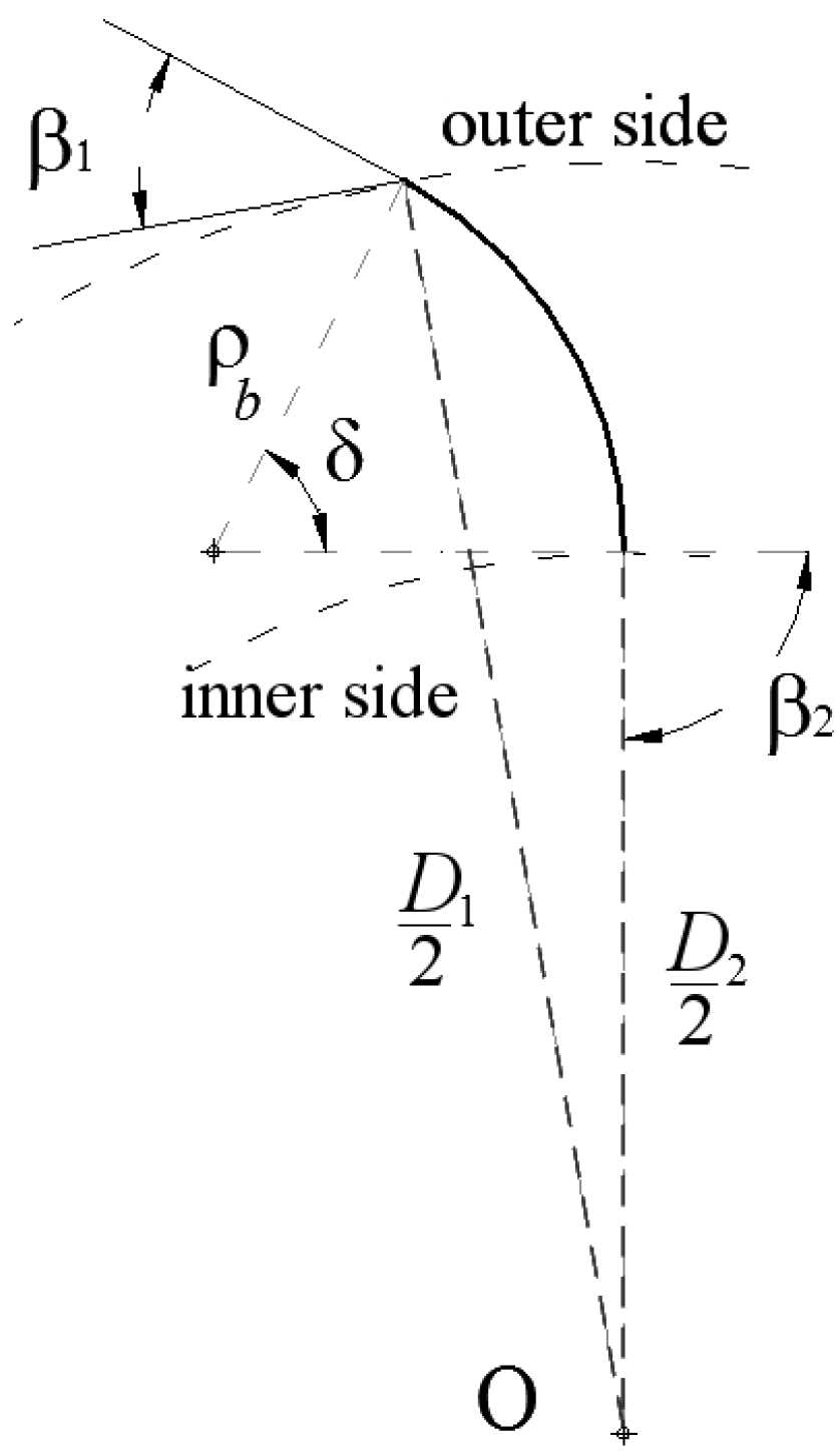
3.1. First Step: Design of Basic Parameters

3.2. Second Step: Impeller Parameters Optimization

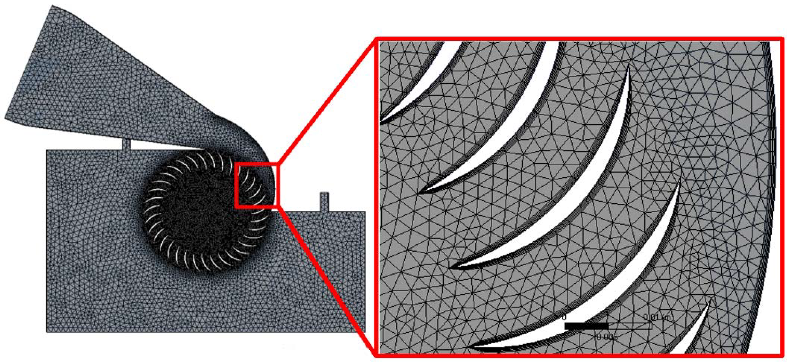
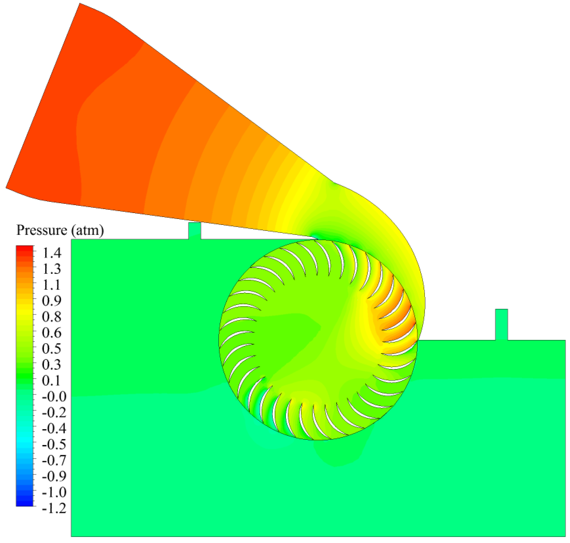
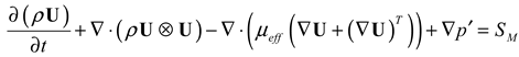
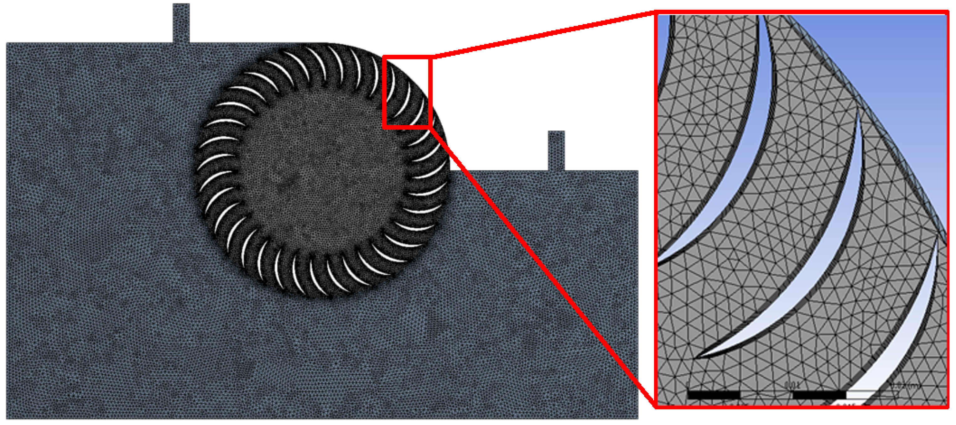
4. Fluid Dynamic Investigation by CFX Code

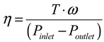
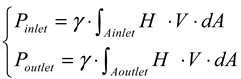
5. Impeller Design Testing
| Parameter | value | Description of the geometrical parameters |
|---|---|---|
| D1 (mm) | 161 | Impeller outer perimeter diameter |
| D2 (mm) | 109 | Impeller inner perimeter diameter |
| Nb (-) | 35 | Number of blades |
| λ (°) | 90 | Inlet discharge angle |
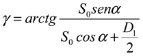
| α (°) | 22 | Attack angle of the outlet nozzle velocity |
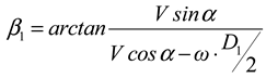
| β1 (°) | 38.9 | Angle between the blade and the outer perimeter of the impeller |
| β2 (°) | 90.0 | Angle between the blade and the inner perimeter of the impeller |
| ρb (mm) | 27.7 | Radius of blade |
| δ (°) | 61.5 | Central angle of blade |
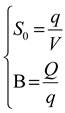
| S0 (mm) | 47 | Nozzle initial height |
| B (mm) | 93 | Nozzle width |
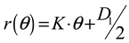
| K (-) | 31.5 | Constant in Equation (19) |
| W (mm) | 139 | Impeller width |
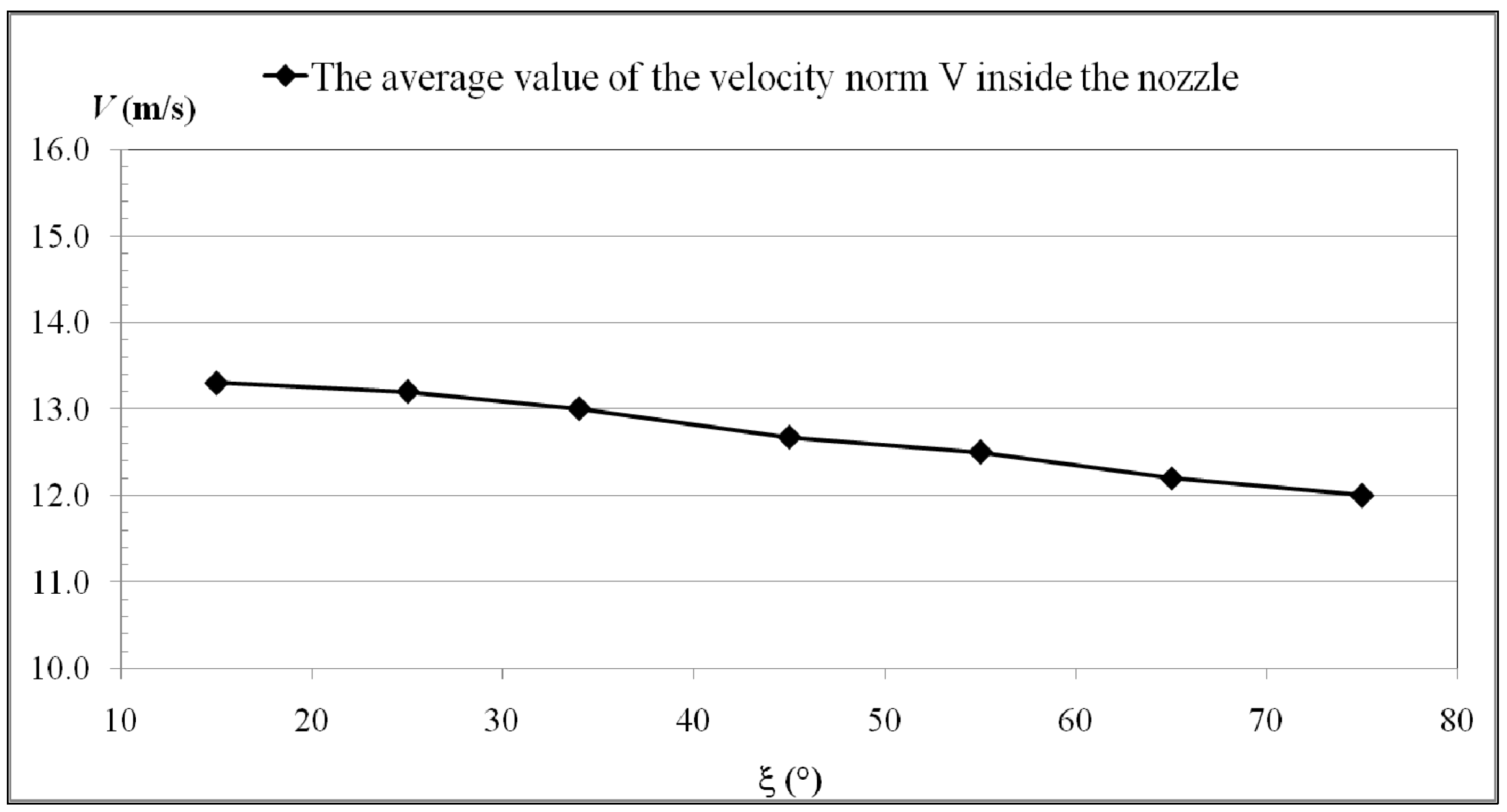
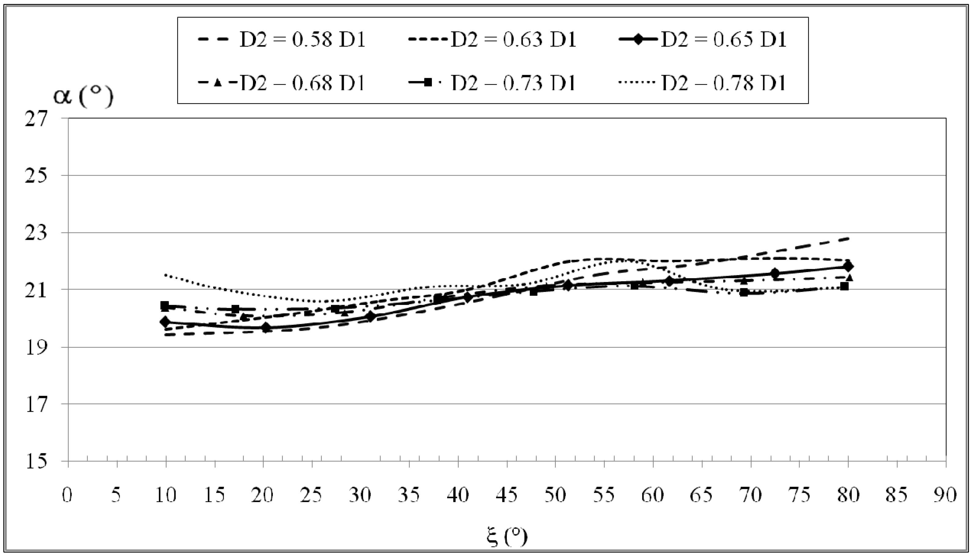
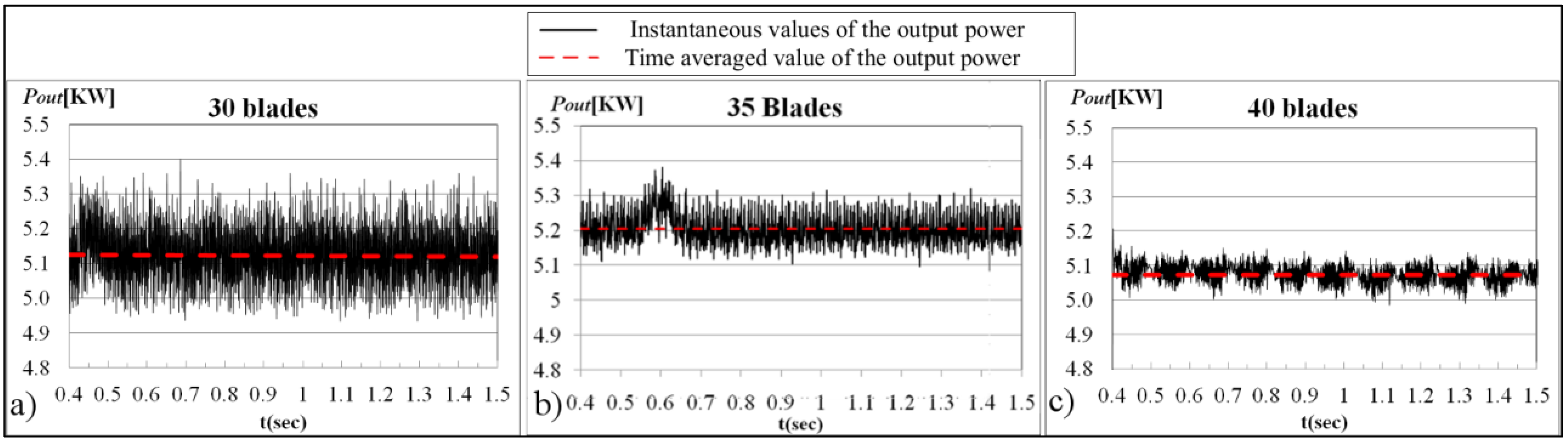
5.1. 2D-Simulations: Optimum Geometry Tests

| D2/D1 | ρb (mm) | δ (degree) |
|---|---|---|
| 0.58 | 34 | 66 |
| 0.63 | 31 | 63 |
| 0.65 | 30 | 63 |
| 0.68 | 28 | 61 |
| 0.73 | 24 | 60 |
| 0.78 | 20 | 58 |


| Parameter | Value | Description of the geometrical parameters |
|---|---|---|
| D1 (mm) | 161 | Impeller outer perimeter diameter |
| D2 (mm) | 104 | Impeller inner perimeter diameter |
| Nb (-) | 35 | Number of blades |
| λ (°) | 90 | Inlet discharge angle |
| α (°) | 22 | Angle of attack |
| β1 (°) | 38.9 | Angle between the blade and the outer perimeter of the impeller |
| β2 (°) | 90.0 | Angle between the blade and the inner perimeter of the impeller |
| ρb (mm) | 29.8 | Radius of blade |
| δ (°) | 62.6 | Central angle of blade |
| S0 (mm) | 47 | The nozzle initial height |
| B (mm) | 93 | Nozzle width |
| K (-) | 31.5 | Constant in Equation (16) |
| W(mm) | 139 | Impeller width (using W/B = 1.5) |
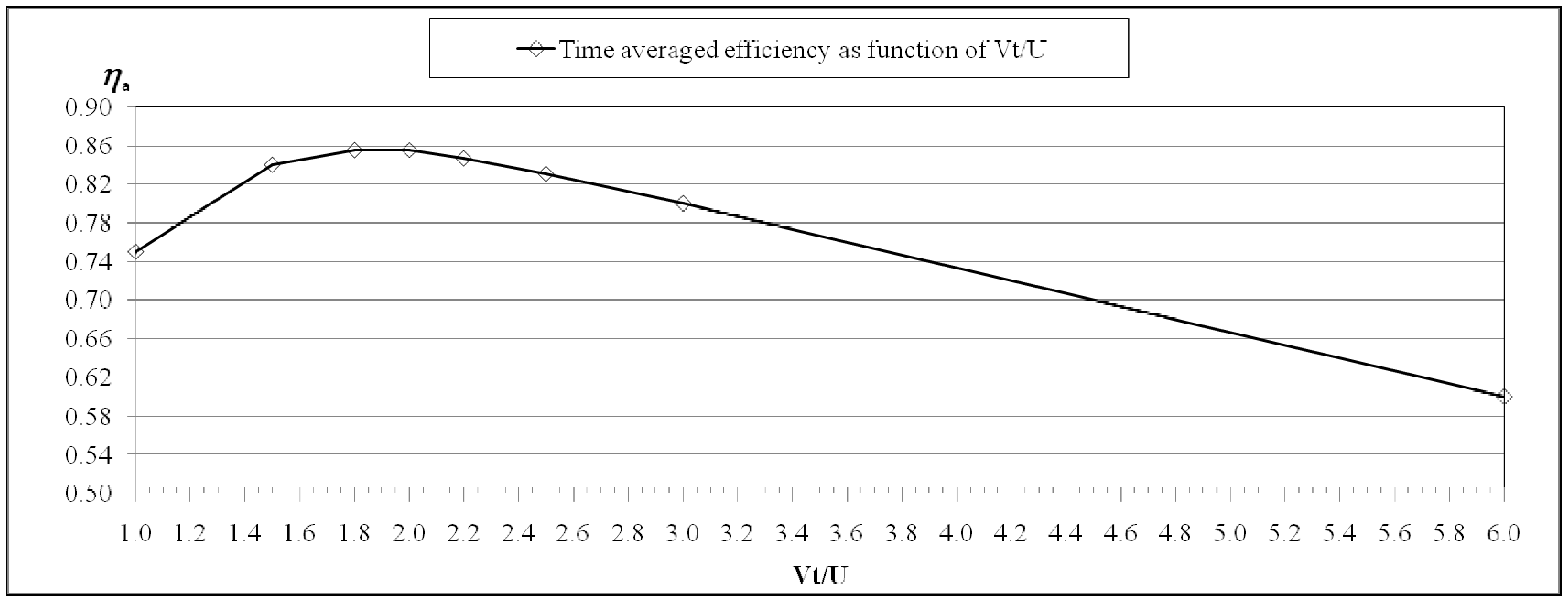
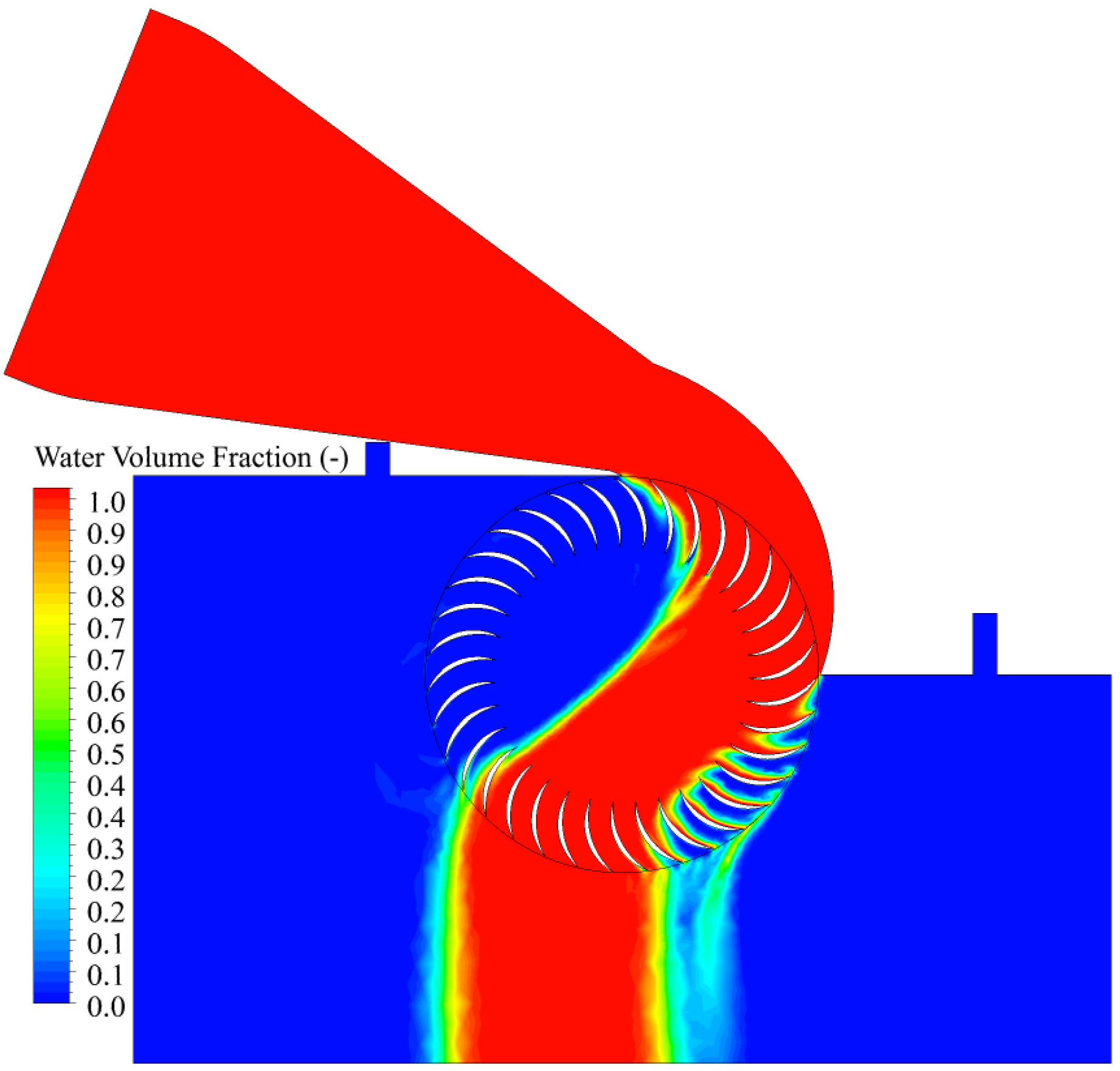

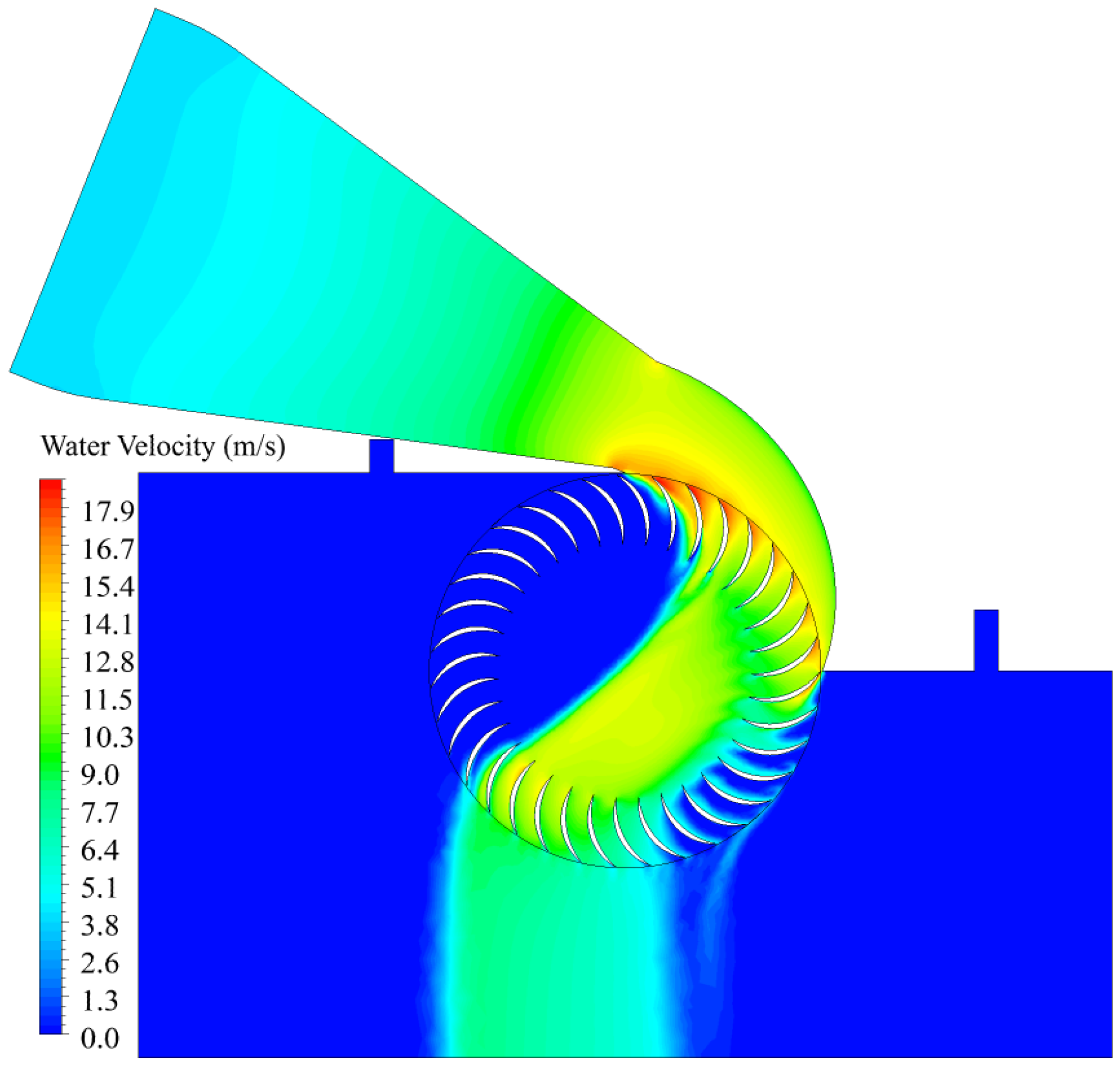
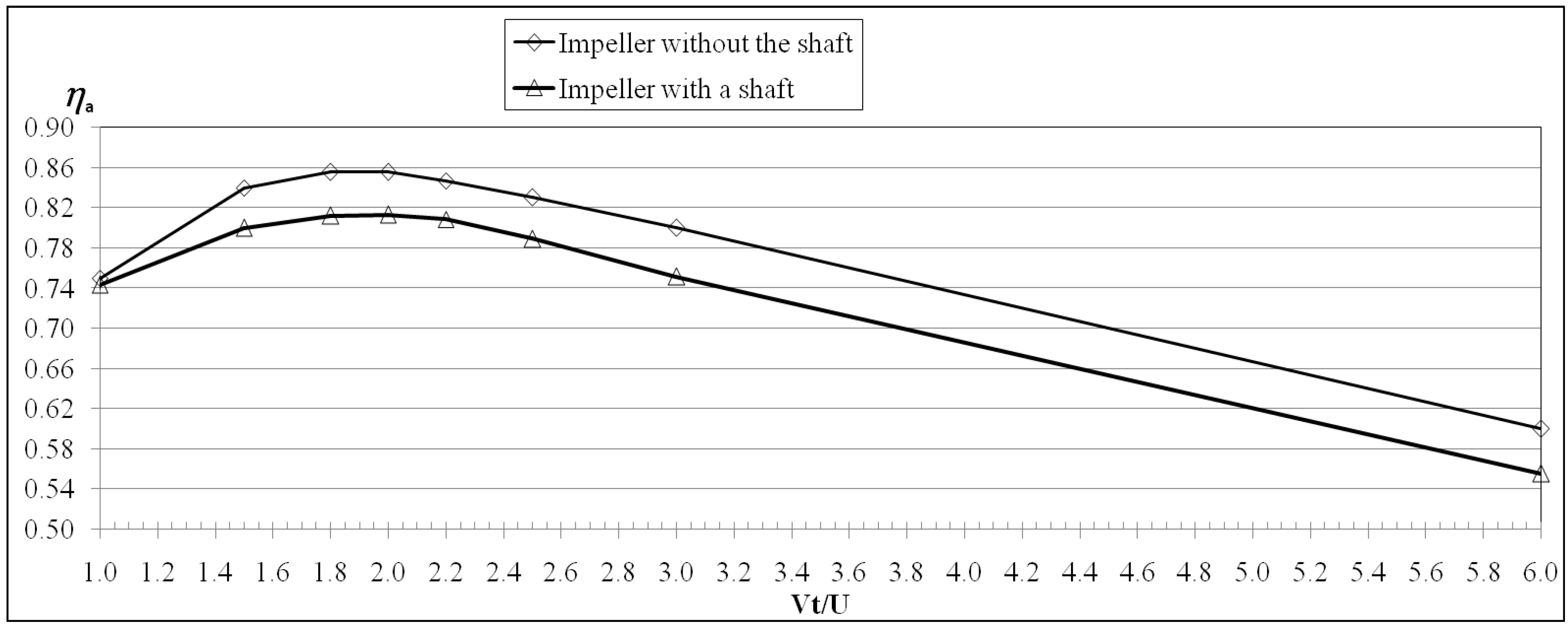

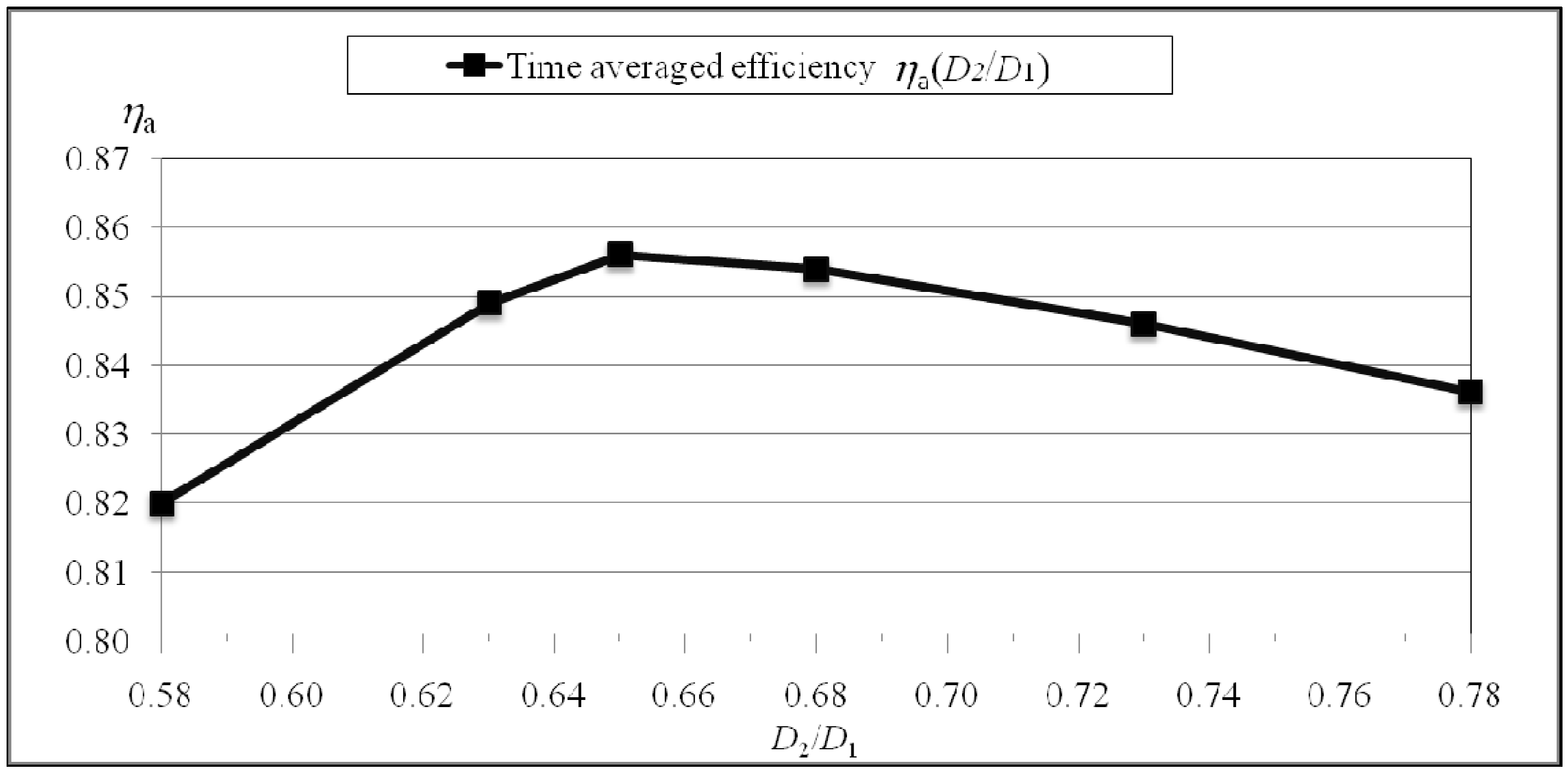
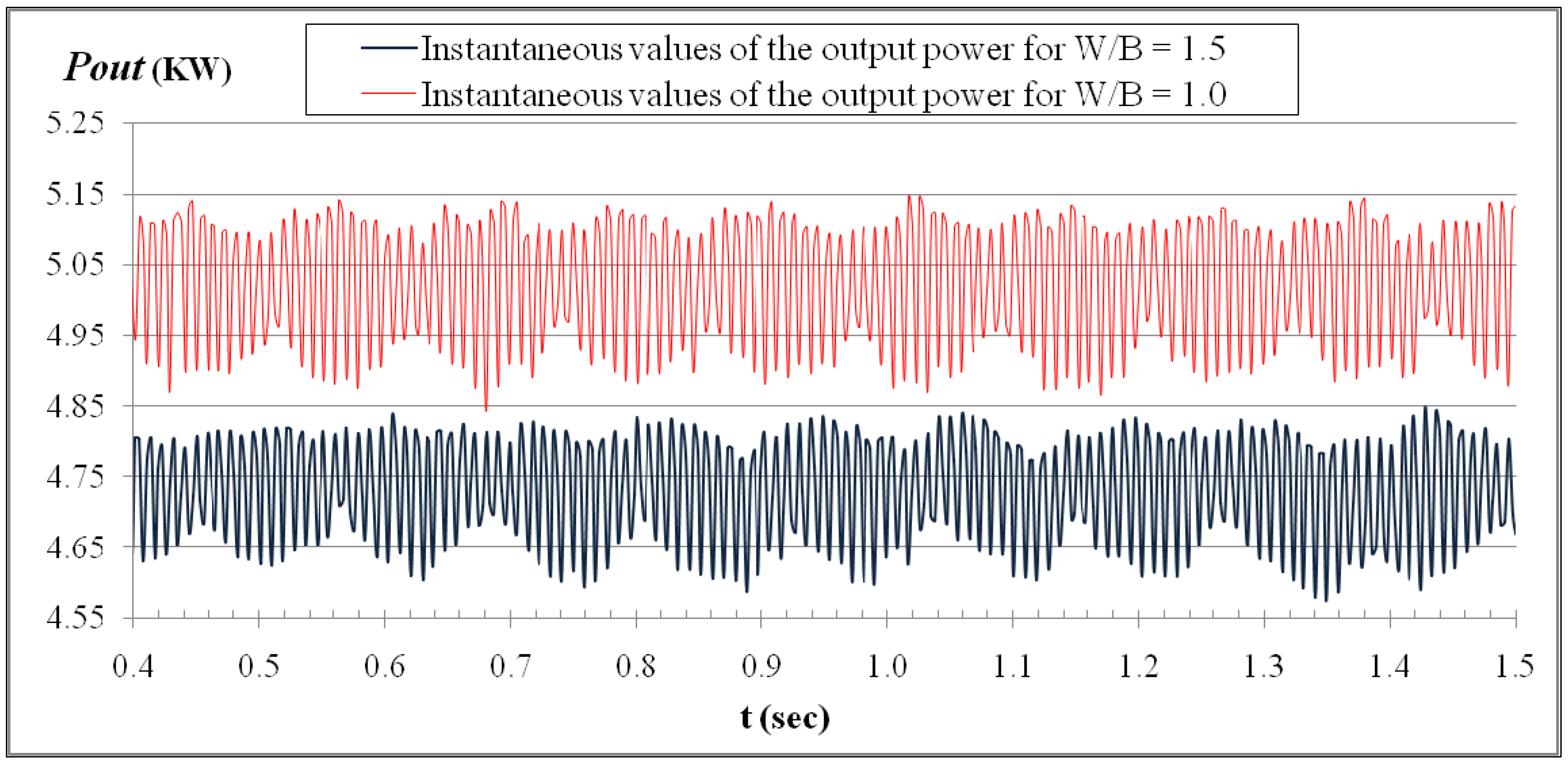
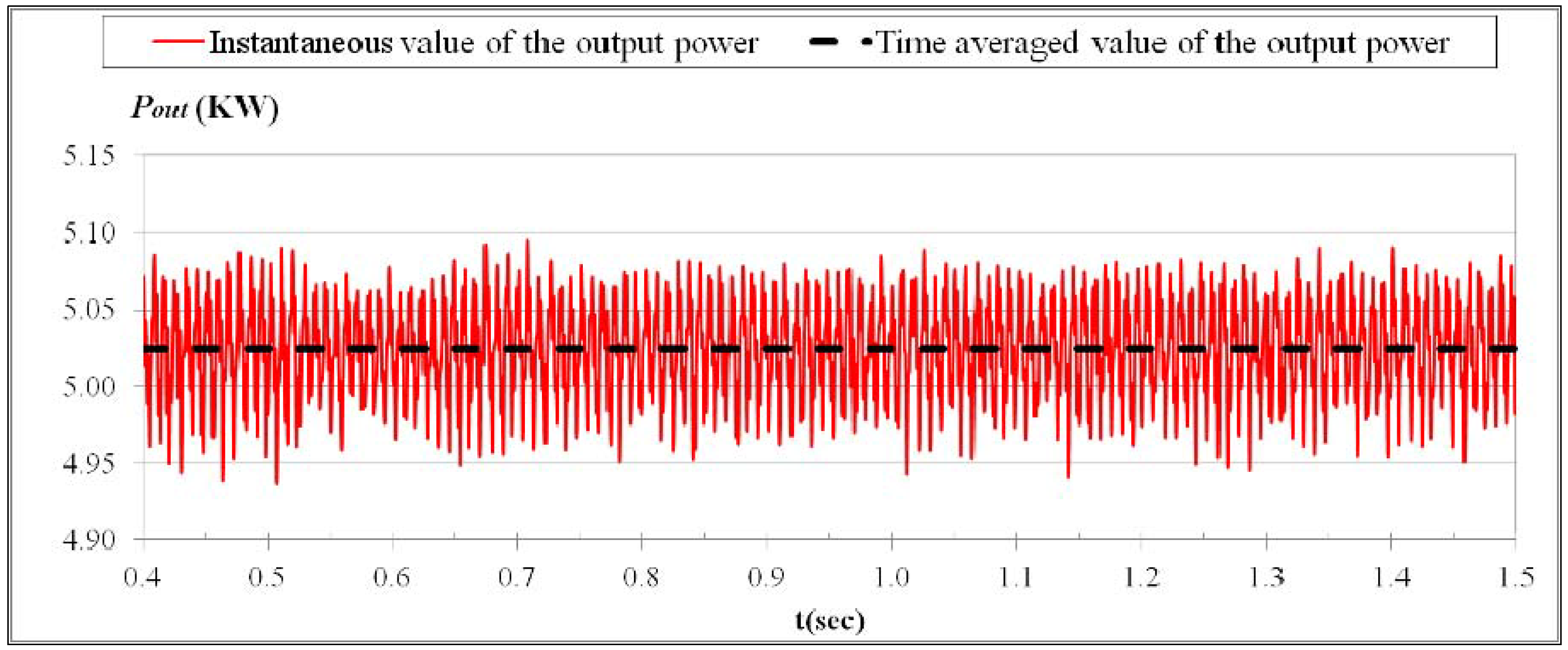
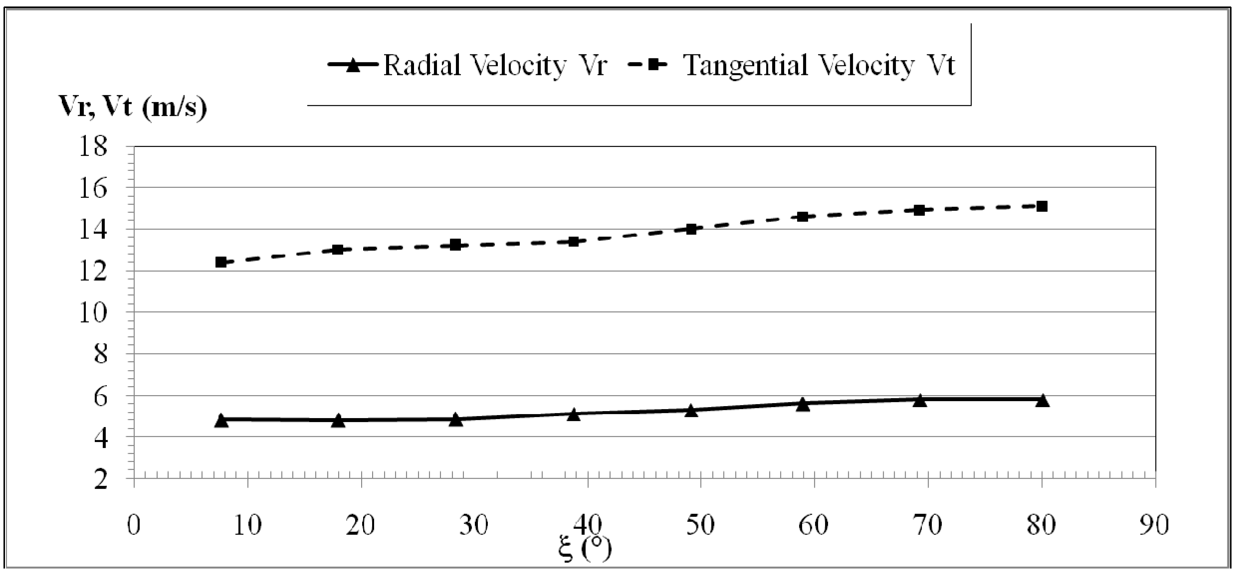
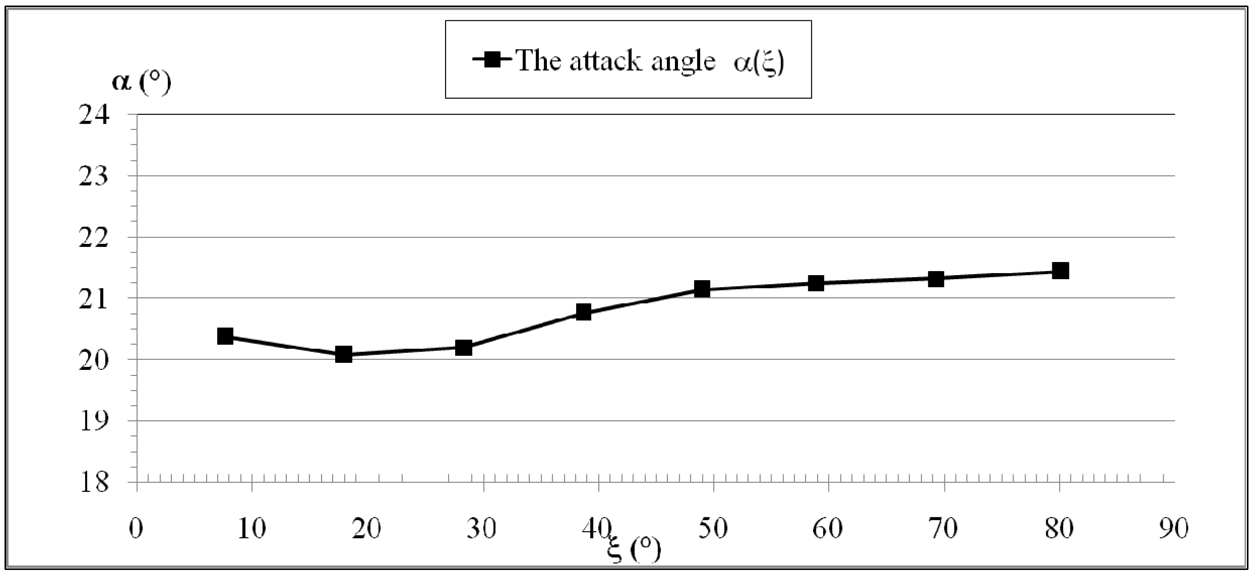
5.2. 3D-Simulations: Spread Ratio Tests

6. Conclusions
Acknowledgments
References
- Anagnostopoulos, J.S.; Papantonis, D.E. Optimal sizing of a run-of-river small hydropower plant. Energy Convers. Manag. 2007, 48, 2663–2670. [Google Scholar] [CrossRef]
- Hosseinia, S.M.H.; Forouzbakhshb, F.; Rahimpoora, M. Determination of the optimal installation capacity of small hydro-power plants through the use of technical, economic and reliability indices. Energy Policy 2005, 33, 1948–1956. [Google Scholar] [CrossRef]
- Carravetta, A.; del Giudice, G.; Fecarotta, O.; Ramos, H. Energy production in water distribution networks: A PAT design strategy. Water Resour. Manag. 2012, 2012, 26, 3947–3959. [Google Scholar] [CrossRef]
- Carravetta, A.; del Giudice, G.; Fecarotta, O.; Ramos, H. PAT Design strategy for energy recovery in water distribution networks by electrical regulation. Energies 2013, 6, 411–424. [Google Scholar] [CrossRef]
- Chapallaz, J.M.; Eichenberger, P. Guida Pratica per la Realizzazione di Piccole Centrali Idrauliche [in Italian]. Ufficio federale dei problemi congiunturali: Berne, Switzerland, 1992; ISBN 3-905232-20-0 (French ver.); ISBN 3-905232-38-3 (Italian ver.). [Google Scholar]
- Penche, C. Guide on How to Develop a Small Hydropower Plant; European Small Hydropower Association: Brussels, Belgium, 2004. [Google Scholar]
- Khosrowpanah, S.; Albertson, M.L.; Fiuzat, A.A. Historical overview of cross-flow turbine. Int. Water Power Dam Constr. 1984, 36, 38–43. [Google Scholar]
- Fiuzat, A.A.; Akerkar, B.P. The Use of Interior Guide Tube in Cross Flow Turbines. In Proceedings of the International Conference on Hydropower-WATERPPOWER ’89, London, UK, 21–26 August 1989.
- Fiuzat, A.A.; Akerkar, B.P. Power outputs of two stages of cross-flow turbine. J. Energy Eng. 1991, 117, 57–70. [Google Scholar] [CrossRef]
- Aziz, N.M.; Desai, V.R. A Laboratory Study to Improve the Efficiency of Cross-Flow Turbines. In Engineering Report; Department of Civil Engineering, Clemson University: Clemson, SC, USA, 1993. [Google Scholar]
- De Andrade, J.; Curiel, C.; Kenyery, F.; Aguillón, O.; Vásquez, A.; Asuaje, M. Numerical investigation of the internal flow in a Banki turbine. Int. J. Rotating Mach. 2011, 841214:1–841214:12. [Google Scholar]
- Mockmore, C.A.; Merryfield, F. The Banki Water Turbine. In Bullettin Series, Engineering Experiment Station; Oregon State System of Higher Education, Oregon State College: Corvallis, OR, USA, 1949. [Google Scholar]
- Aziz, N.M.; Totapally, H.G.S. Design Parameter Refinement for Improved Cross-Flow Turbine Performance. In Engineering Report; Departement of Civil Engineering, Clemson University: Clemson, SC, USA, 1994. [Google Scholar]
- Choi, Y.; Lim, J.; Kim, Y.; Lee, Y. Performance and internal flow characteristics of a cross-flow hydro turbine by the shapes of nozzle and runner blade. J. Fluid Sci. Technol. 2008, 3, 398–409. [Google Scholar] [CrossRef]
- Hothersall, R.J. Micro hydro: Turbine selection criteria. Int. Water Power Dam Constr. 1984, 36, 26–29. [Google Scholar]
- Khosrowpanah, S.; Fiuzat, A.A.; Albertson, M.L. Experimental study of cross-flow turbine. J. Hydraul. Eng. 1988, 114, 299–314. [Google Scholar] [CrossRef]
- Desai, V.R.; Aziz, N.M. An experimental investigation of cross-flow turbine efficiency. J. Fluid Eng. 1994, 116, 45–550. [Google Scholar] [CrossRef]
- Nakase, Y.; Fukatomi, J.; Watanaba, T.; Suetsugu, T.; Kubota, T.; Kushimoto, S. A Study of Cross-flow Turbine (Effects of Nozzle Shape on its Performance). In Proceedings of the Winter Annual Meeting A.S.M.E., Phoenix, AZ, USA, 14–19 November 1982; Webb, D.R., Papadakis, C., Eds.; In Small Hydro Power Fluid Machinery; American Society of Mechanical Engineers (ASME): New York, NY, USA. 1982; pp. 13–18. [Google Scholar]
- Ansys Inc. ANSYS CFX Reference Guide; Ansys Inc.: Canonsburg, PA, USA, 2006. [Google Scholar]
© 2013 by the authors; licensee MDPI, Basel, Switzerland. This article is an open access article distributed under the terms and conditions of the Creative Commons Attribution license (http://creativecommons.org/licenses/by/3.0/).
Share and Cite
Sammartano, V.; Aricò, C.; Carravetta, A.; Fecarotta, O.; Tucciarelli, T. Banki-Michell Optimal Design by Computational Fluid Dynamics Testing and Hydrodynamic Analysis. Energies 2013, 6, 2362-2385. https://doi.org/10.3390/en6052362
Sammartano V, Aricò C, Carravetta A, Fecarotta O, Tucciarelli T. Banki-Michell Optimal Design by Computational Fluid Dynamics Testing and Hydrodynamic Analysis. Energies. 2013; 6(5):2362-2385. https://doi.org/10.3390/en6052362
Chicago/Turabian StyleSammartano, Vincenzo, Costanza Aricò, Armando Carravetta, Oreste Fecarotta, and Tullio Tucciarelli. 2013. "Banki-Michell Optimal Design by Computational Fluid Dynamics Testing and Hydrodynamic Analysis" Energies 6, no. 5: 2362-2385. https://doi.org/10.3390/en6052362