Exploring Ventilation Efficiency in Poultry Buildings: The Validation of Computational Fluid Dynamics (CFD) in a Cross-Mechanically Ventilated Broiler Farm

Abstract

Broiler production in modern poultry farms commonly uses mechanical ventilation systems. This mechanical ventilation requires an amount of electric energy and a high level of investment in technology. Nevertheless, broiler production is affected by periodic problems of mortality because of thermal stress, thus being crucial to explore the ventilation efficiency. In this article, we analyze a cross-mechanical ventilation system focusing on air velocity distribution. In this way, two methodologies were used to explore indoor environment in livestock buildings: Computational Fluid Dynamics (CFD) simulations and direct measurements for verification and validation (V&V) of CFD. In this study, a validation model using a Generalized Linear Model (GLM) was conducted to compare these methodologies. The results showed that both methodologies were similar in results: the average of air velocities values were 0.60 ± 0.56 m s⁻¹ for CFD and 0.64 ± 0.54 m s⁻¹ for direct measurements. In conclusion, the air velocity was not affected by the methodology (CFD or direct measurements), and the CFD simulations were therefore validated to analyze indoor environment of poultry farms and its operations. A better knowledge of the indoor environment may contribute to reduce the demand of electric energy, increasing benefits and improving the thermal comfort of broilers.

1. Introduction

In many areas, broiler production is affected every year by several episodes of massive bird mortality because of the confluence of high temperature and humidity values during summer seasons. This problem causes great economical losses and animal suffering, which is inconceivable in a modern society, which uses a high technological investment at these poultry farms and establishes regulations to ensure animal welfare. In the last decades, mechanical ventilation was incorporated at intensive poultry farms to improve the thermal comfort of the animals [1,2], but the problems related with heat stress have not been solved yet [3,4]. Cross-mechanical ventilation is widely used in poultry farms but the problems of mortality and broiler stress appears more frequently in hot and humid climates, especially in summer. For this reason, it is crucial to explore thoroughly the efficiency of these ventilation systems in order to improve the whole livestock building design and to improve their indoor environment. Whereas natural ventilation does not consume electric energy to force air exchange, mechanical ventilation requires a certain amount of energy to activate the fans, the automation of inlets and other electric/electronic facilities. Obviously, an optimization of energy consumption is desired to reduce farm costs and to reduce the demand of electric energy. A great percentage of electric energy is provided by fossil fuels, nuclear or other non renewable sources. A reduction of electric energy consumption in livestock farms can be achieved by optimizing livestock building design and improving ventilation efficiency by an appropriate management. This may contribute to reduce costs for farmers, and indirectly may reduce the consumption of fossil fuel or other non-renewable sources contributing to the control of the global warming. In agricultural systems such as greenhouses or farms, two methodologies are used to analyze problems related to the indoor environment: direct measurements by the suitable electronic instrumentation and Computational Fluid Dynamics (CFD) techniques. The CFD procedures are very emergent techniques in many fields of science and engineering. However, it is necessary a suitable instrumentation system to validate the simulations. Whereas CFD techniques and associate instrumentation are widely developed in other fields of engineering (e.g., aerodynamic, automotive, spatial, chemistry, nuclear, simulation of fire...), in agricultural engineering they are less developed, particularly in the study of indoor environments of farms. A possible reason for this fact is that direct measurements by means of multi-sensor systems for poultry farms are complex and they have not been tested with great success yet [5]. Previous research has focused on the design of sensors and data acquisition systems to measure the environmental parameters according with the ranges and particularities of these complex buildings (large dimensions, automatisms of fans and air-inlets, feeding and watering equipment, refrigerating and heating systems…), which is essential to carry out the validation. A robust measurement system adapted to the hard environmental conditions at poultry farms was designed, which allowed data acquisition at conditions of isotemporality at multiple points [5]. Such a system is necessary to validate CFD measurements due to the great sudden fluctuations of air velocity in time and space generated at mechanical ventilation.

Broiler production offers meat at reasonable price to the consumers and in the current context of economic crisis the consumption of broiler meat is increasing due to its price-quality relation. In this sense, poultry meat must maintain its quality, reducing mortality and other costs. Intensive production normally takes place at mechanically ventilated farms that with a high level of investment which allows a high density of animals and more thermal comfort in comparison with naturally ventilated farms. In this way, housing conditions is acknowledged to influence animal welfare more than animal density [6]. In the European Union (EU), a specific regulation related to intensive production and welfare of broilers has been developed (EU Council Directive 2007/43/EC) [7]. According to this Directive, the countries of EU must ensure that broiler facilities are constructed and operated to provide the animals with a proper environment in terms of temperature, relative humidity and gases (ammonia and carbon dioxide). Several studies have demonstrated the influence of thermal effects on the broiler performance: [8] studied the effects of air and temperature on broiler performance; [9] studied the effect of air velocity on broiler performance and feed and water consumption; [10] affirmed that the air velocity alters the broiler performance under harsh environmental conditions; [11] studied the poultry responses to heat stress; [12] studied the effects of high-air velocity on broiler performance; [13] studied the ventilation, sensible heat loss, broiler energy and water balance under harsh environmental conditions.

In mechanically ventilated broiler buildings, farmers usually control the indoor environment by changing the geometry of inlets and the activity of fans. These changes are carried out by automatisms that cause changes in the differential pressure and as a consequence, fluctuations in the air velocity values and directions are originated. These changes of air velocity are used to regulate the heat exchange of the broilers with their environment. For the farmers, modifying animal housing conditions is relatively simple using pressure difference, but normally, the farmer experience is a key factor to provide the animals with proper ventilation. However, to the moment very scarce information is available on how to optimize ventilation, not only in terms of air exchange, but also of velocity distribution. As a consequence, massive deaths due to thermal stress still occur in hot conditions. For this reason, the CFD techniques will not be only used to find optimal design for poultry buildings and improve their thermal comfort; they will also be used to analyze the best poultry farms operations under the strong premise that economizes electric energy.

In a general context of livestock buildings, CFD techniques have been already applied [14,15,16,17]. Furthermore, it can found some applications of CFD simulations applied specifically at poultry farms [18,19,20].

The validation of CFD simulations is an important rule [21]. In this sense, it is essential to ensure that CFD can be used to explore trends of poultry farm design and its optimal operations in practice. For laying hens, [20] studied a mechanical ventilated building using the commercial code CFD FLUENT [22]. Similarly, [18] studied a transversal, mechanically ventilated broiler farm with the same commercial code. However, they only used three measurement points in a single mobile support that had to be changed by an operator. In their experiment, the number of measurement points was reduced and the presence of an operator to change the mobile post could distort the airflow and air velocity values and trajectories [23].

This study aims to validate CFD simulations of air velocity with direct measurements of a multi-sensor system. As the fluctuations of values and trajectories of air velocity is the most expanded method to control thermal comfort at poultry farms with forced ventilation systems, this paper focuses on the validation of the CFD-air velocity results with the direct measurements performed in a broiler farm located in the Valencia Community (Spain).

2. Materials and Methods

2.1. Experimental Poultry Farm

Measurements and simulations were carried out at a commercial broiler farm located in Villarreal (Northern Hemisphere, Latitude 39°56’, Longitude 0°6’; 43 m above sea level) in Eastern Spain. The poultry building used forced ventilation by negative-pressure systems, in particular, a mechanical cross-ventilation system. Dimensions were: length, 110 m; width, 12.60 m; sidewall height 2.6 m; roof 21.53%, total height of the building 4 m. There were nine large exhaust fans (diameter 1.28 m) and seven small exhaust fans (diameter 0.68 m) installed, described in [5]. The building was empty during the experimentation to avoid the possible interferences due to the presence of the animals in the airflow circuit and to prevent the inconveniences that the measuring system could cause in animal performance.

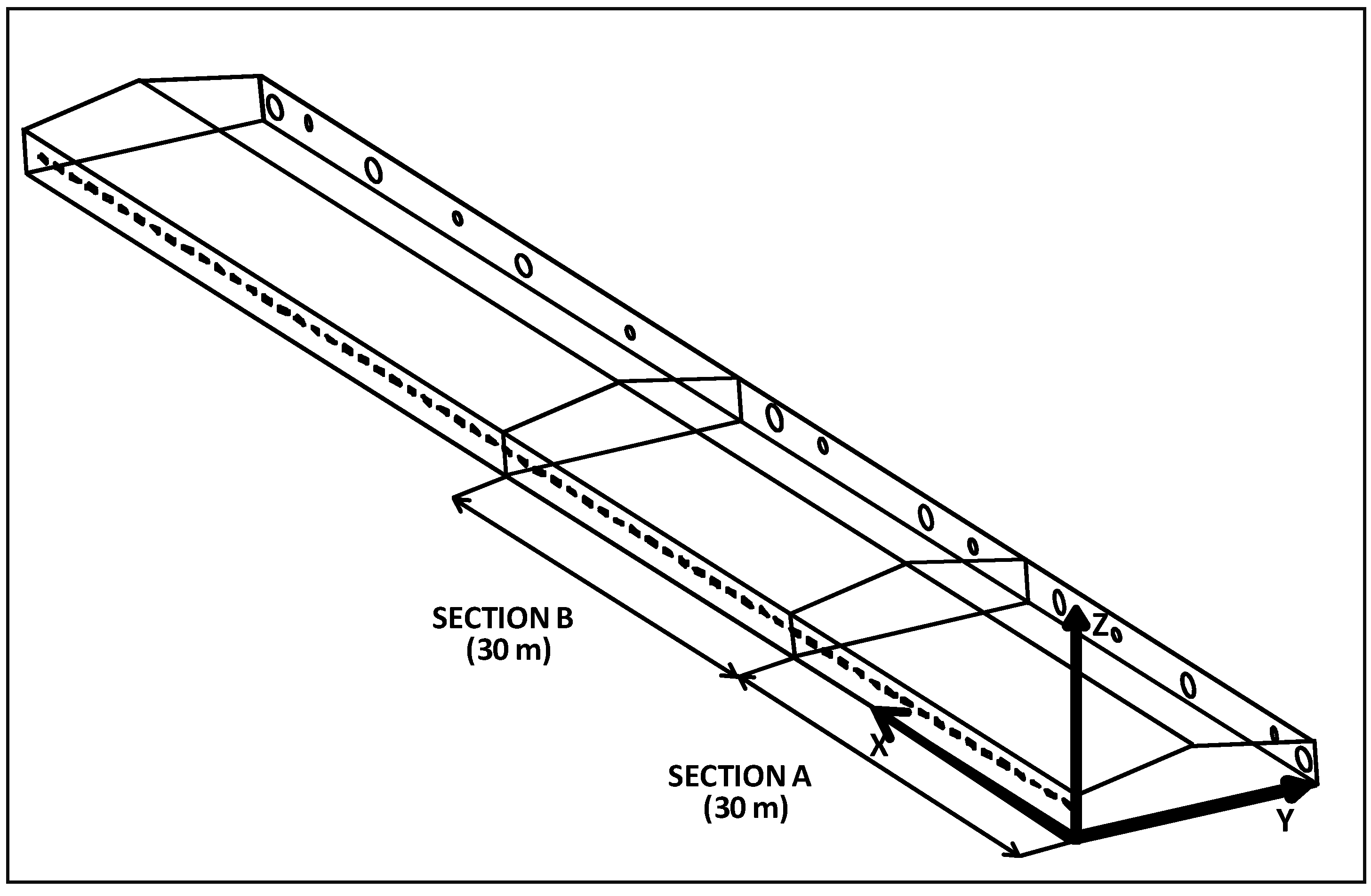
2.2. Test Sections and Multisensor System for Direct Measurements

Field experiments were conducted in two sections of the poultry farm of similar length (30 m). As shown in Figure 1, the first section was located near one extreme of the building (Section A), whereas the second corresponded to the center of the building (Section B). A multisensor system for isotemporal measurements to assess indoor climatic conditions in poultry farms was used to measure air velocity. The measurement system was composed by 24 air velocity sensors, 24 temperature sensors and 2 differential pressure sensors [5] and was able to acquire up to a maximum of 128 signals simultaneously at 5 s intervals obtaining one data of each sensor at a frequency of this 5 s (10 min in each section and in each Boundary Condition). In the two studied sections measurements were taken at two heights (0.25 m—birds’ level—and 1.75 m) using 12 tripods. The location of the sensors was chosen according to the situation of inlets and fans and the sensor’s coordinates are shown in Table 1. During the field experiment, a total of 23,040 measurements were taken in the same day at four scenarios and two sections of the poultry farm in 24 points of each section and eight CFD simulations for the same scenario and section where done.

Figure 1. Test sections in the experimental poultry farm.

Figure 1. Test sections in the experimental poultry farm.

Table 1. Coordinates of sensors.

Sensor number *	Section A		Section B
	X-coordinate (m)	Y-coordinate (m)	X-coordinate (m)	Y-coordinate (m)
1–2	22.45	0.30	35.90	0.05
3–4	19.50	12.00	31.50	11.80
5–6	18.00	11.95	32.80	11.95
7–8	9.30	12.00	41.80	7.15
9–10	5.70	12.05	40.70	6.80
11–12	0.60	12.00	45.85	11.35
13–14	0.55	6.30	47.35	4.50
15–16	0.50	7.60	46.95	5.35
17–18	0.55	2.15	44.05	0.80
19–20	8.70	6.70	48.50	3.15
21–22	24.85	7.10	47.70	1.10
23–24	23.60	7.15	47.70	0.65

*: The first sensors at animal level, the second at 1.75 m.

Table 1. Coordinates of sensors.

Sensor number *	Section A		Section B
	X-coordinate (m)	Y-coordinate (m)	X-coordinate (m)	Y-coordinate (m)
1–2	22.45	0.30	35.90	0.05
3–4	19.50	12.00	31.50	11.80
5–6	18.00	11.95	32.80	11.95
7–8	9.30	12.00	41.80	7.15
9–10	5.70	12.05	40.70	6.80
11–12	0.60	12.00	45.85	11.35
13–14	0.55	6.30	47.35	4.50
15–16	0.50	7.60	46.95	5.35
17–18	0.55	2.15	44.05	0.80
19–20	8.70	6.70	48.50	3.15
21–22	24.85	7.10	47.70	1.10
23–24	23.60	7.15	47.70	0.65

*: The first sensors at animal level, the second at 1.75 m.

2.3. CFD Background

The commercial software FLUENT [22] was used to realize all the CFD simulations. The geometry model and mesh were developed using the pre-processor Gambit [24] (Geometry and Mesh Building Intelligent Toolkit) of FLUENT. CFD FLUENT was used at previous CFD simulations of poultry farms as mentioned before [18,19,20].

The basic idea of all CFD techniques is the resolution of a set of partial differential Equations (PDE’s) [16,25] that corresponded to Equations of continuity [Equation (1)], conservation of momentum (Navier-Stokes’s law) [Equation (2)] and Equation of the energy [Equation (3)].

Those Equations for an uncompressible fluid with isothermal properties are:

(1)

(2)

(3)

where ρ: fluid density (kg m⁻³); t: time (s); x, x_i, x_j: length components (m); u_i, u_j: velocity component (m s⁻¹); p: pressure (Pa); τ_ij: stress tensor (Pa); g_i: gravitational acceleration (m s⁻²); F_i: external body forces in the i direction (N m⁻³); c: specific heat (W kg⁻¹ K⁻¹); T: temperature (K); K: thermal conductivity (W m⁻¹ K⁻¹ ); S_T: thermal source term (W m⁻³).

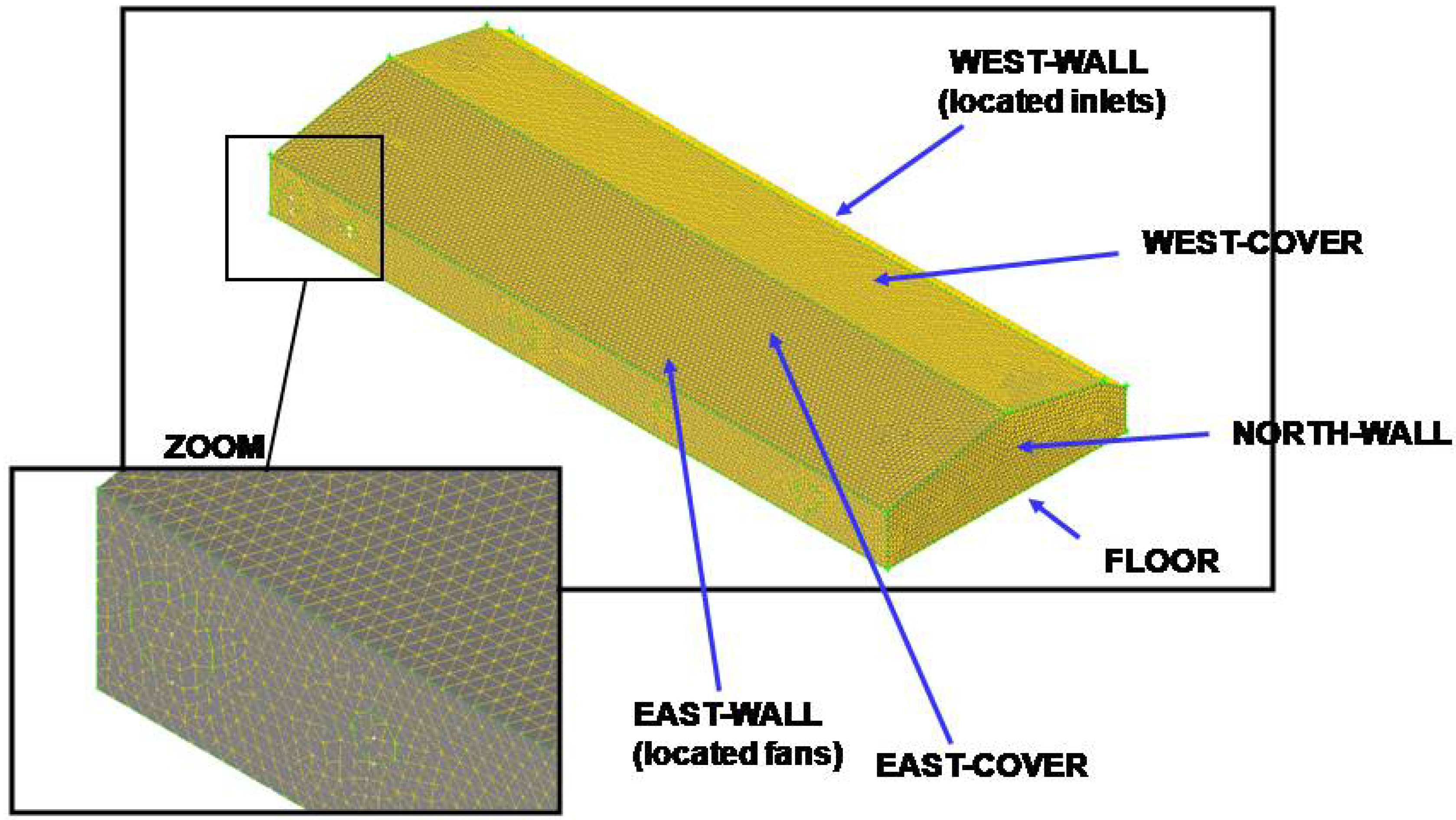
2.4. Turbulence Models and Boundary Conditions (BC)

CFD FLUENT [22] has various available turbulence models: Inviscid, laminar, Spallard-Allmaras, standard k-ε, k-ε RNG, k-ε realizable, Reynolds Stress Model (RSM), standard k-ω, SST k-ω and Large Eddy Simulation (LES). Reynolds averaged Navier-Stokes Equations (RANS) determine the effect of turbulence on the mean flow field through time averaging [16]; LES forms a solution given the fact that large turbulent eddies are highly anisotropic on both the mean velocity gradients and geometry of the flow domain [16]. LES needs higher computing time and powerful computers and it is used for specific purposes when extreme accuracy is required. It should be noted that none of the existing turbulence models are complete, i.e., their prediction performance is highly reliant on turbulent flow and geometry [16]. Traditionally, in agricultural engineering, (greenhouses and livestock buildings), the turbulence models commonly used were: standard k-ε, k-ε RNG, k-ε realizable and Reynolds Stress Model (RSM). In this paper, the standard k-ε model described by [26] was used, also considering that [18] also used it in their CFD simulations in a cross-mechanical ventilated poultry farm. This model is widely used in engineering for agricultural applications such as the modeling of poultry farms [18,19,20], because it is considered robust and reasonably accurate. The Equations of transport of this turbulence model were (4) and (5) [22]:

(4)

(5)

where k: turbulent kinetic energy (m² s⁻²); μ: fluid viscosity (m² s); μ_t: turbulent viscosity (m² s); σ_k: turbulent Prandtl number for k; G_k: the generation of kinetic energy due to the variations of the components of the average velocity of the flow (kg m⁻¹ s⁻²); G_b: the generation of kinetic energy by boundary push (kg m⁻¹ s⁻²); ε: turbulent dissipation rate (m² s⁻³); Y_M: contribution of the pulsatile expansion associated to the compressible turbulence (kg m⁻¹ s⁻²); σ_ε: turbulent Prandtl number for ε; C_1ε: constant; C_2ε: constant; C_3ε= tanh[u₁/u₂]; u₁: velocity of flow parallel to g_i (gravitational vector); u₂: velocity of flow perpendicular to g_i. Moreover, the constant values were C_1ε = 1.44, C_2ε = 1.92, σ_k = 1.0 and σ_ε = 1.3 [22,26].

In this paper, we carried out eight final three-dimensional CFD simulations that corresponded with the four scenarios tested (four typical conditions of operation at two sections of the poultry farm). Each scenario was mainly characterized by the number of fans operating and the different opening of inlets, the differential pressure [5] and the ventilation rate was measured [27] in each trial scenario. From these scenarios were obtained the BC to introduce at CFD software.

Each final simulation was adopted when the numerical solutions were stabilized through successive numerical simulations increasing the density and refinement of the mesh (grid independence). As we have indicated above, the pre-processor GAMBIT [24] was used to build the computational domain with these meshes assigning (without the numerical value) the BC’s at each surface and volume. To assure a good quality of the mesh (mainly composed by tetrahedral cells), the equiangular skewness of GAMBIT [24] was used. For a good quality of the mesh, this value must be less than 0.8 [24]:

(6)

where θ_max= Largest angle in face or cell; θ_min= Smallest angle in face or cell; θ_e= Angle for equiangular face or cell.

The mesh domain built in GAMBIT [24] was exported to the CFD-solver FLUENT [22], which solved the above mentioned governing partial differential Equations of continuity [Equation (1)], of momentum [Equation (2)] and energy [Equation (3)] in each mesh of the computational domain. The pressure and velocity coupling is solved by the SIMPLE algorithm [25] with the second order upwind scheme [25]. The k-ε standard turbulence model and wall functions [22] were used in the CFD simulations.

It was assumed that the flow is steady, three-dimensional, viscous, turbulent, incompressible and isothermal. The properties of the fluid (air in this case) are considered constants and their values were shown in Table 2. Gravitational acceleration was also considered.

Table 2. Main inputs and BC at CFD simulations.

(i) Constant and computational settings
3D double precision Segregated Steady Turbulence model: Standard k-ε Wall treatment: Standard Wall Functions Pressure-velocity coupling: SIMPLE algorithm Discretization scheme: Pressure: standard; Momentum: Second order upwind; Turbulence kinetic energy: Second order upwind; Turbulence dissipation rate: Second order upwind; Energy: Second order upwind. Air properties: Density: 1.225 Kg m−3; Cp: 1006.43 J kg−1 K−1; Thermal conductivity: 0.0242 W m−1 K−1; Viscosity: 1.789·10−5 kg m−1s−1. Wall material: Density: 2400 Kg m−3; Cp= 1125 J kg−1 K−1; Thermal conductivity: 1.2 W m−1 K−1. Atmospheric pressure: 101,325 Pa. Gravitational acceleration: 9.81 m s−2.
(ii) Boundary Conditions
CFD Simulation	Assay Section	Scenario	Outlets (Fans) Mass Flux rate at each outlet (in kg s−1) Air temperature at each outlet (in K)	Inlet Air (10% Turbulence Intensity (1)) Air velocity (in m s−1) Air temperature (in K)	Temperature at solid elements (in K) Floor North-Wall (2) South-Wall (2) East-Wall (2) West-Wall (2) East-Cover (2) West-Cover (2)
I	Section A	I	Large = 9.60 Kg s−1 303.7 K Small = 0	6.62 m s−1 304.5 K	303.0 K 303.4 K 304.7 K 305.1 K 304.1 K 305.5 K 305.0 K
II	Section A	II	Large = 9.03 Kg s−1 301.9 K Small = 3.2 Kg s−1 301.9 K	7.70 m s−1 303.3 K	303.0 K 302.5 K 303.0 K 303.5 K 302.0 K 303.5 K 302.0 K
III	Section A	III	Large = 8.17 Kg s−1 303.7 K Small = 0	9.01 m s−1 304.5 K	302.0 K 303.4 K 304.6 K 306.6 K 303.1 K 305.7 K 305.0 K
IV	Section A	IV	Large = 7.82 Kg s−1 301.9 K Small = 2.78 Kg s−1 301.9 K	10.67 m s−1 303 K	303.0 K 302.5 K 303.0 K 304.0 K 302.0 K 303.5 K 302.0 K
V	Section B	I	Large = 9.60 Kg s−1 304.8 K Small = 0	4.66 m s−1 305.6 K	305.0 K 305.0 K 306.0 K 307.0 K 303.0 K 305.0 K 304.0 K
(ii) Boundary Conditions
VI	Section B	II	Large = 9.03 Kg s−1 305.1 K Small = 3.2 Kg s−1 305.1 K	5.93 m s−1 305.8 K	304.0 K 304.0 K 306.0 K 307.3 K 303.5 K 305.7 K 304.6 K
VII	Section B	III	Large = 8.17 Kg s−1 304.9 K Small = 0	6.35 m s−1 305.8 K	304.0 K 304.5 K 306.0 K 307.2 K 303.2 K 305.5 K 304.3 K
VIII	Section B	IV	Large = 7.89 Kg s−1 305.1 K Small = 2.78 Kg s−1 305.1 K	8.23 m s−1 306.2 K	304.0 K 304.0 K 306.0 K 307.5 K 303.5 K 305.3 K 304.7 K

(1) Turbulence intensity is defined by [22] as the ratio of the root-mean-square of the velocity fluctuations, u_fluct , to the mean flow velocity, u_aver; (2) According to the main orientation reached by the walls and covers.

Table 2. Main inputs and BC at CFD simulations.

(i) Constant and computational settings
3D double precision Segregated Steady Turbulence model: Standard k-ε Wall treatment: Standard Wall Functions Pressure-velocity coupling: SIMPLE algorithm Discretization scheme: Pressure: standard; Momentum: Second order upwind; Turbulence kinetic energy: Second order upwind; Turbulence dissipation rate: Second order upwind; Energy: Second order upwind. Air properties: Density: 1.225 Kg m−3; Cp: 1006.43 J kg−1 K−1; Thermal conductivity: 0.0242 W m−1 K−1; Viscosity: 1.789·10−5 kg m−1s−1. Wall material: Density: 2400 Kg m−3; Cp= 1125 J kg−1 K−1; Thermal conductivity: 1.2 W m−1 K−1. Atmospheric pressure: 101,325 Pa. Gravitational acceleration: 9.81 m s−2.
(ii) Boundary Conditions
CFD Simulation	Assay Section	Scenario	Outlets (Fans) Mass Flux rate at each outlet (in kg s−1) Air temperature at each outlet (in K)	Inlet Air (10% Turbulence Intensity (1)) Air velocity (in m s−1) Air temperature (in K)	Temperature at solid elements (in K) Floor North-Wall (2) South-Wall (2) East-Wall (2) West-Wall (2) East-Cover (2) West-Cover (2)
I	Section A	I	Large = 9.60 Kg s−1 303.7 K Small = 0	6.62 m s−1 304.5 K	303.0 K 303.4 K 304.7 K 305.1 K 304.1 K 305.5 K 305.0 K
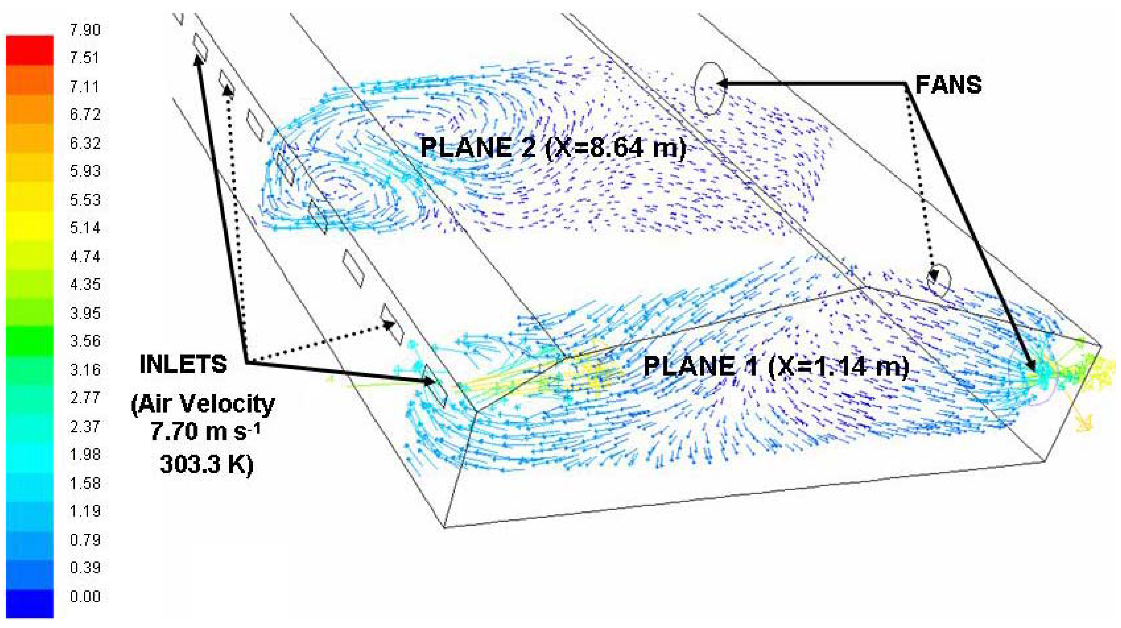
II	Section A	II	Large = 9.03 Kg s−1 301.9 K Small = 3.2 Kg s−1 301.9 K	7.70 m s−1 303.3 K	303.0 K 302.5 K 303.0 K 303.5 K 302.0 K 303.5 K 302.0 K
III	Section A	III	Large = 8.17 Kg s−1 303.7 K Small = 0	9.01 m s−1 304.5 K	302.0 K 303.4 K 304.6 K 306.6 K 303.1 K 305.7 K 305.0 K
IV	Section A	IV	Large = 7.82 Kg s−1 301.9 K Small = 2.78 Kg s−1 301.9 K	10.67 m s−1 303 K	303.0 K 302.5 K 303.0 K 304.0 K 302.0 K 303.5 K 302.0 K
V	Section B	I	Large = 9.60 Kg s−1 304.8 K Small = 0	4.66 m s−1 305.6 K	305.0 K 305.0 K 306.0 K 307.0 K 303.0 K 305.0 K 304.0 K
(ii) Boundary Conditions
VI	Section B	II	Large = 9.03 Kg s−1 305.1 K Small = 3.2 Kg s−1 305.1 K	5.93 m s−1 305.8 K	304.0 K 304.0 K 306.0 K 307.3 K 303.5 K 305.7 K 304.6 K
VII	Section B	III	Large = 8.17 Kg s−1 304.9 K Small = 0	6.35 m s−1 305.8 K	304.0 K 304.5 K 306.0 K 307.2 K 303.2 K 305.5 K 304.3 K
VIII	Section B	IV	Large = 7.89 Kg s−1 305.1 K Small = 2.78 Kg s−1 305.1 K	8.23 m s−1 306.2 K	304.0 K 304.0 K 306.0 K 307.5 K 303.5 K 305.3 K 304.7 K

(1) Turbulence intensity is defined by [22] as the ratio of the root-mean-square of the velocity fluctuations, u_fluct , to the mean flow velocity, u_aver; (2) According to the main orientation reached by the walls and covers.

Mass flux rate (in kg s⁻¹) of each outlet (fan), air velocity at inlets and temperature at solid elements were BC used to carry out the CFD simulations. The air temperature was also measured at inlets and at outlets, as the temperature fluctuations at inlets and at outlets were negligible in each scenario (operation), one average from air temperature at inlets and another average from air temperature at outlets was introduced as indicates in Table 2. In the same way, two averages of mass flux rate (one average from each type of fans) and another average of air velocity at inlets from each scenario were introduced at CFD software as indicated in Table 2. These air velocity at inlets (m s⁻¹) were obtained from thirty measurements (thirty seconds) at each inlet by means of a calibrated Testo 425 hot-wire anemometer [28]; then, the average of all inlets was calculated and introduced in CFD software. Introducing these single values reduces time consumption of CFD calculations; in this sense, some authors have calculated and assumed uniform velocities and airflow rates for inlets or outlets in their CFD simulations [18,29,30]. In this paper, the individual ventilation rate of each outlet was measured by [27]. This protocol of measurement [27] consist of ducted the exhaust air 50 cm from the fan and then by means of a hot wire anemometer measuring at 24 different locations in the section [31]. On the other hand, the surface temperature of internal solid elements (wall, floor or covers) was measured by means of a portable model Optex PT-3LF non-contact (infrared) thermometer and the measured values were indicated in the same Table 2. Evidently, the specifications of a correct functioning of this model of thermometer were according to the range of values reached of any poultry farm from broiler production (an accuracy ±1 of the reading value or ±2 °C ±1 digit in an ambient temperature 0 °C to 50 °C, ambient humidity 35% to 85% RH). The temperatures reached at solid elements were another BC requires by CFD program. Table 2 summarizes the main inputs and BC at CFD simulations.

Geometry and mesh were developed using GAMBIT [24]. The CFD models were discretized in finite volumes in unstructured meshes as shown in Figure 2. For practical reasons of nomenclature expression of some BC (temperature at walls and covers), the terms North-Wall, South-Wall, East-Wall, West-Wall, East-Cover, West-Cover and floor will be used, according to the physical orientation as seen in Figure 2.

Figure 2. Screen of geometry and meshed of poultry farm at GAMBIT (FLUENT). Orientation of walls and covers.

Figure 2. Screen of geometry and meshed of poultry farm at GAMBIT (FLUENT). Orientation of walls and covers.

The big exhaust fans and the small exhaust fans were modeled as circles of diameter 1.28 m and 0.68 m respectively (its real dimensions). The inlets were modeled for each scenario following the actual geometry adopted by the inlet windows. As the poultry farm was empty during the scenarios, the broiler metabolism and other elements such feeding and watering equipment were not modeled.

Model CFD locations with special interest were those corresponding to the location of the sensors, which coordinates were specified in the Table 1.

2.5. Statistical Validation Model

The validation consisted of a statistical treatment between CFD-air velocity results and the direct measurements with the multi-sensor system, by means of an analysis of variance (ANOVA).

The model used to do this validation was:

(7)

where the different variables are explained below, and in brackets the number of levels within each variable is indicated:

• Y_ijk: Air velocity in the section i at boundary conditions j at height k by the sensor l and by methodology n;
• Z_i: Measurement section (2);
• B_j: Boundary conditions (4);
• H_k: Height of the sensor (2);
• SN_l: Sensor l (24);
• M_n: Methodology: CFD vs. direct measurements using the multisensor system (2);
• (Z X B)_ij: Interaction between Section-Boundary (8);
• (Z X H)_ik: Interaction between Section-Height (4);
• (Z X M)_in: Interaction between Section-Methodology (4);
• (Z X SN)_il: Interaction between Section-Sensor (48);
• (B X H)_jk: Interaction between Boundary-Height (8);
• (B X SN)_jl: Interaction between Boundary-Sensor (96);
• (B X M)_jn: Interaction between Boundary-Methodology (8);
• (H X M)_lk: Interaction between Height-Methodology (4);
• (SN X H)_lk: Interaction between Sensor-Height (48);
• (Z X B X H)_ijk: Triple interaction between Section-Boundary-Height (16);
• (Z X SN X M)_iln: Triple interaction between Section-Sensor-Methodology (96);
• (B X SN X M)_jln: Triple interaction between Boundary-Sensor-Methodology (192);
• (Z X B X H X M)_ijkn: Four interaction between Section-Boundary-Height-Methodology (384);
• ε_ijkln: Error of the model

For observing the effect of the methodology (CFD or direct measurements) all factors are considered random, the model was analyzed by the GLM procedure of SAS Systems [32]. It was considered that a factor has a statistically significant influence on a variable when the p-value obtained for this valor in the analysis of variance is equal or lower than 0.05. On the contrary, higher p-values indicate that a factor has no significant influence.

3. Results and Discussion

3.1. CFD vs. Direct Measurements

CFD-air velocity results and its direct measurements using the multisensor system are shown in Table 3.

As shown in Table 3 minor differences were found between CFD results and direct measurements using the multi-sensor system. It has not appreciated any significant tendency in the results using both methodologies. The more discrepant case (CFD vs. direct measurements) was in scenario II at 0.25 m (broiler’s level) obtaining 0.70 ± 0.35 m s⁻¹ from measurements and 0.60 ± 0.30 m s⁻¹ from CFD.

Table 3. Air velocity in m s⁻¹ (mean ± standard deviation) in the field experiment by direct measurements and by CFD simulations. The number of data is indicated in parenthesis.

Scenario	Height	Methodology	Section A	Section B	Mean
I	0.25 m	Measured	0.62 ± 0.86 (12)	0.37 ± 0.30 (12)	0.50 ± 0.65 (24)
		CFD	0.52 ± 0.68 (12)	0.34 ± 0.29 (12)	0.43 ± 0.52 (24)
	1.75 m	Measured	0.37 ± 0.39 (12)	0.66 ± 1.00 (12)	0.52 ± 0.76 (24)
		CFD	0.35 ± 0.40 (12)	0.62 ± 0.97 (12)	0.49 ± 0.74 (24)
	Mean	Measured	0.50 ± 0.67 (24)	0.53 ± 0.74 (24)	0.51 ± 0.70 (48)
		CFD	0.43 ± 0.55 (24)	0.48 ± 0.71 (24)	0.46 ± 0.63 (48)
II	0.25 m	Measured	0.70 ± 0.35 (12)	0.71 ± 0.29 (12)	0.71 ± 0.33 (24)
		CFD	0.60 ± 0.30 (12)	0.74 ± 0.36 (12)	0.67 ± 0.33 (24)
	1.75	Measured	0.47 ± 0.32 (12)	0.68 ± 0.47 (12)	0.58 ± 0.41 (24)
		CFD	0.41 ± 0.34 (12)	0.68 ± 0.50 (12)	0.55 ± 0.44 (24)
	Mean	Measured	0.59 ± 0.35 (24)	0.70 ± 0.38 (24)	0.64 ± 0.37 (48)
		CFD	0.60 ± 0.30 (24)	0.71 ± 0.43 (24)	0.61 ± 0.39 (48)
III	0.25 m	Measured	0.78 ± 0.41 (12)	0.80 ± 0.31 (12)	0.79 ± 0.35 (24)
		CFD	0.73 ± 0.36 (12)	0.89 ± 0.43 (12)	0.75 ± 0.36 (24)
	1.75 m	Measured	0.63 ± 0.34 (12)	0.77 ± 0.50 (12)	0.70 ± 0.42 (24)
		CFD	0.50 ± 0.32 (12)	0.79 ± 0.55 (12)	0.65 ± 0.47 (24)
	Mean	Measured	0.71 ± 0.37 (24)	0.79 ± 0.41 (24)	0.75 ± 0.39 (48)
		CFD	0.62 ± 0.35 (24)	0.84 ± 0.49 (24)	0.73 ± 0.44 (48)
IV	0.25 m	Measured	0.42 ± 0.26 (12)	0.65 ± 0.59 (12)	0.54 ± 0.46 (24)
		CFD	0.37 ± 0.27 (12)	0.54 ± 0.38 (12)	0.46 ± 0.34 (24)
	1.75 m	Measured	0.72 ± 0.69 (12)	0.77 ± 0.87 (12)	0.74 ± 0.75 (24)
		CFD	0.72 ± 0.87 (12)	0.80 ± 1.04 (12)	0.76 ± 0.94 (24)
	Mean	Measured	0.57 ± 0.53 (24)	0.71 ± 0.71 (24)	0.64 ± 0.62 (48)
		CFD	0.54 ± 0.65 (24)	0.67 ± 0.78 (24)	0.61 ± 0.71(48)
All	0.25 m	Measured	0.63 ± 0.53 (48)	0.63 ± 0.41 (48)	0.63 ± 0.47 (96)
		CFD	0.55 ± 0.44 (48)	0.63 ± 0.41 (48)	0.59 ± 0.43 (96)
	1.75 m	Measured	0.55 ± 0.47 (48)	0.72 ± 0.71 (48)	0.63 ± 0.61 (96)
		CFD	0.50 ± 0.53 (48)	0.72 ± 0.78 (48)	0.61 ± 0.67 (96)
	Mean	Measured	0.59 ± 0.50 (96)	0.68 ± 0.58 (96)	0.63 ± 0.54 (192)
		CFD	0.52 ± 0.49 (96)	0.68 ± 0.62 (96)	0.60 ± 0.56 (192)

Table 3. Air velocity in m s⁻¹ (mean ± standard deviation) in the field experiment by direct measurements and by CFD simulations. The number of data is indicated in parenthesis.

Scenario	Height	Methodology	Section A	Section B	Mean
I	0.25 m	Measured	0.62 ± 0.86 (12)	0.37 ± 0.30 (12)	0.50 ± 0.65 (24)
		CFD	0.52 ± 0.68 (12)	0.34 ± 0.29 (12)	0.43 ± 0.52 (24)
	1.75 m	Measured	0.37 ± 0.39 (12)	0.66 ± 1.00 (12)	0.52 ± 0.76 (24)
		CFD	0.35 ± 0.40 (12)	0.62 ± 0.97 (12)	0.49 ± 0.74 (24)
	Mean	Measured	0.50 ± 0.67 (24)	0.53 ± 0.74 (24)	0.51 ± 0.70 (48)
		CFD	0.43 ± 0.55 (24)	0.48 ± 0.71 (24)	0.46 ± 0.63 (48)
II	0.25 m	Measured	0.70 ± 0.35 (12)	0.71 ± 0.29 (12)	0.71 ± 0.33 (24)
		CFD	0.60 ± 0.30 (12)	0.74 ± 0.36 (12)	0.67 ± 0.33 (24)
	1.75	Measured	0.47 ± 0.32 (12)	0.68 ± 0.47 (12)	0.58 ± 0.41 (24)
		CFD	0.41 ± 0.34 (12)	0.68 ± 0.50 (12)	0.55 ± 0.44 (24)
	Mean	Measured	0.59 ± 0.35 (24)	0.70 ± 0.38 (24)	0.64 ± 0.37 (48)
		CFD	0.60 ± 0.30 (24)	0.71 ± 0.43 (24)	0.61 ± 0.39 (48)
III	0.25 m	Measured	0.78 ± 0.41 (12)	0.80 ± 0.31 (12)	0.79 ± 0.35 (24)
		CFD	0.73 ± 0.36 (12)	0.89 ± 0.43 (12)	0.75 ± 0.36 (24)
	1.75 m	Measured	0.63 ± 0.34 (12)	0.77 ± 0.50 (12)	0.70 ± 0.42 (24)
		CFD	0.50 ± 0.32 (12)	0.79 ± 0.55 (12)	0.65 ± 0.47 (24)
	Mean	Measured	0.71 ± 0.37 (24)	0.79 ± 0.41 (24)	0.75 ± 0.39 (48)
		CFD	0.62 ± 0.35 (24)	0.84 ± 0.49 (24)	0.73 ± 0.44 (48)
IV	0.25 m	Measured	0.42 ± 0.26 (12)	0.65 ± 0.59 (12)	0.54 ± 0.46 (24)
		CFD	0.37 ± 0.27 (12)	0.54 ± 0.38 (12)	0.46 ± 0.34 (24)
	1.75 m	Measured	0.72 ± 0.69 (12)	0.77 ± 0.87 (12)	0.74 ± 0.75 (24)
		CFD	0.72 ± 0.87 (12)	0.80 ± 1.04 (12)	0.76 ± 0.94 (24)
	Mean	Measured	0.57 ± 0.53 (24)	0.71 ± 0.71 (24)	0.64 ± 0.62 (48)
		CFD	0.54 ± 0.65 (24)	0.67 ± 0.78 (24)	0.61 ± 0.71(48)
All	0.25 m	Measured	0.63 ± 0.53 (48)	0.63 ± 0.41 (48)	0.63 ± 0.47 (96)
		CFD	0.55 ± 0.44 (48)	0.63 ± 0.41 (48)	0.59 ± 0.43 (96)
	1.75 m	Measured	0.55 ± 0.47 (48)	0.72 ± 0.71 (48)	0.63 ± 0.61 (96)
		CFD	0.50 ± 0.53 (48)	0.72 ± 0.78 (48)	0.61 ± 0.67 (96)
	Mean	Measured	0.59 ± 0.50 (96)	0.68 ± 0.58 (96)	0.63 ± 0.54 (192)
		CFD	0.52 ± 0.49 (96)	0.68 ± 0.62 (96)	0.60 ± 0.56 (192)

3.2. CFD-Air Velocity Results

An advantage of CFD simulations is that they offer a visual representation which gives a comprehensive idea of the trends of airflow in which parameters are represented by colors or vectors at different trial scenarios (operations). Examples of some graphical outputs of CFD simulations are shown in Figure 3 and Figure 4. Figure 3 shows air velocity fields in two vertical planes (Planes 1 and 2) of the section A at Scenario II. Plane 1 was placed in the same center of a fan and inlet and Plane 2 was placed between fans. According to this location, these two planes showed different air velocity distribution as seen in Figure 3.

CFD also provides interesting knowledge of the trajectories of airflow using vectors as shows the Figure 4.

Figure 3. Contours of air velocity in Planes 1 and 2 of the Section A in a trial scenario (Scenario II). Air velocity is expressed in m s⁻¹.

Figure 3. Contours of air velocity in Planes 1 and 2 of the Section A in a trial scenario (Scenario II). Air velocity is expressed in m s⁻¹.

Figure 4. Vectors of air velocity showing trajectories in Planes 1 and 2 of the Figure 3. Air velocity is expressed in m s⁻¹.

Figure 4. Vectors of air velocity showing trajectories in Planes 1 and 2 of the Figure 3. Air velocity is expressed in m s⁻¹.

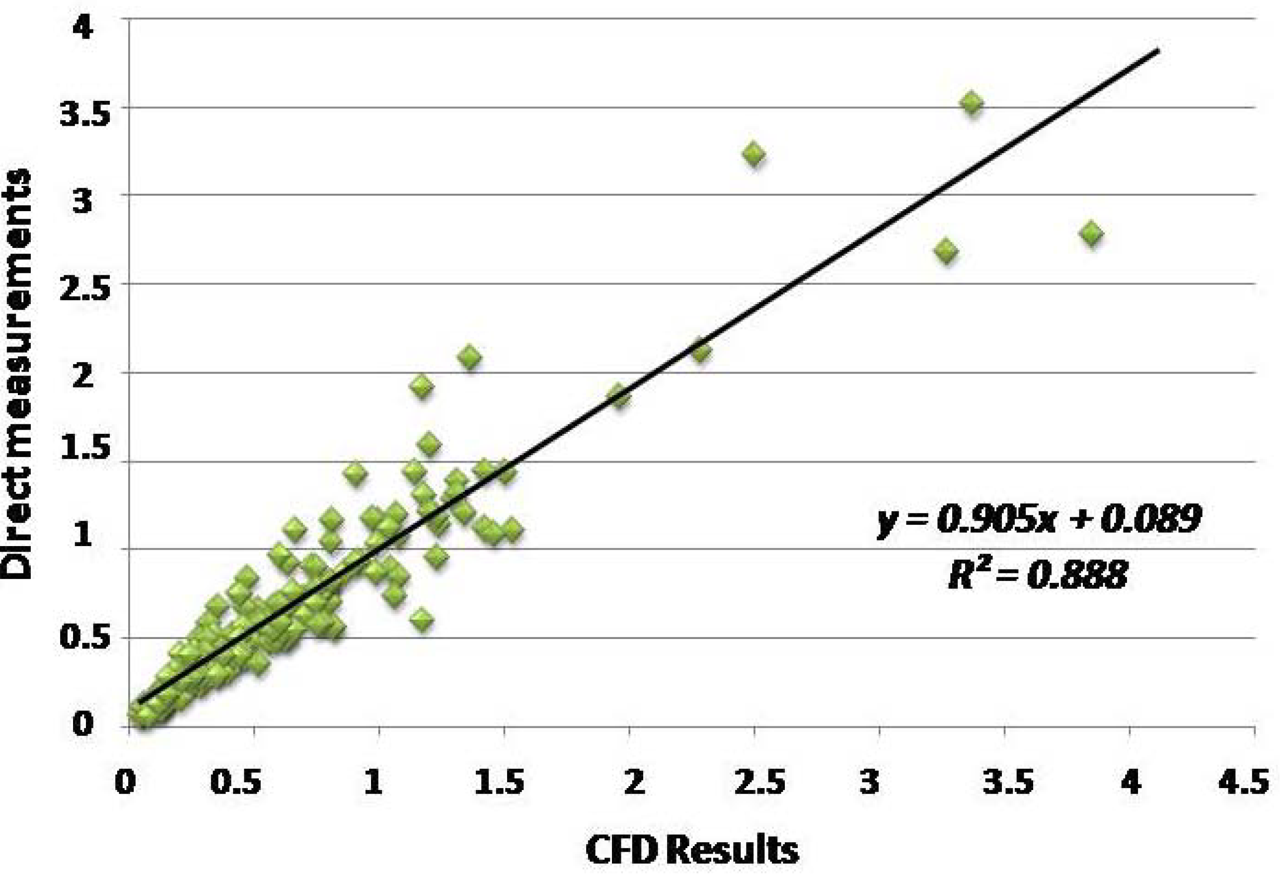
3.3. Results of the Validation Model

Table 4 shows the results of the ANOVA. In this table, the main result is that the variable “Methodology” was not significant (p-value < 0.5271); i.e., it is indifferent using the CFD techniques or the direct measurements using the multisensor system. Using this model, it can be affirmed that the CFD results of air velocity are validated.

Table 4. ANOVA of air velocity at different scenarios.

Parameter	DF	Sum of squares	Mean square	F-ratio	p-value
Section	1	1.31	1.32	2.94	0.4895
Boundary	3	3.16	1.05	1.87	0.4551
Height	1	0.01	0.01	0.02	0.9184
Sensor	22	34.83	1.58	0.89	0.6041
Methodology	1	0.11	0.11	0.46	0.5271
Section × Boundary	3	0.24	0.08	0.20	0.8884
Section × Height	1	0.59	0.59	0.36	0.5574
Section × Methodology	1	0.11	0.11	–1.92	-
Section × Sensor	22	30.31	1.38	51.55	<0.0001
Boundary × Height	3	2.41	0.80	1.15	0.3829
Boundary × Sensor	66	26.77	0.40	33.98	<0.0001
Boundary × Methodology	3	0.01	0.003	–0.05	-
Height × Methodology	1	0.01	0.01	–0.07	-
Sensor × Height	22	0.66	0.03	–0.47	-
Section × Boundary × Height	3	1.20	0.40	22.12	0.0012
Section × Sensor × Methodology	22	0.59	0.03	0.26	0.9997
Boundary × Sensor × Methodology	66	0.79	0.01	0.12	1.0000
Section × Boundary × Height × Methodology	6	0.11	0.02	0.17	0.9833
Error	132	13.68	0.10	-	-

Table 4. ANOVA of air velocity at different scenarios.

Parameter	DF	Sum of squares	Mean square	F-ratio	p-value
Section	1	1.31	1.32	2.94	0.4895
Boundary	3	3.16	1.05	1.87	0.4551
Height	1	0.01	0.01	0.02	0.9184
Sensor	22	34.83	1.58	0.89	0.6041
Methodology	1	0.11	0.11	0.46	0.5271
Section × Boundary	3	0.24	0.08	0.20	0.8884
Section × Height	1	0.59	0.59	0.36	0.5574
Section × Methodology	1	0.11	0.11	–1.92	-
Section × Sensor	22	30.31	1.38	51.55	<0.0001
Boundary × Height	3	2.41	0.80	1.15	0.3829
Boundary × Sensor	66	26.77	0.40	33.98	<0.0001
Boundary × Methodology	3	0.01	0.003	–0.05	-
Height × Methodology	1	0.01	0.01	–0.07	-
Sensor × Height	22	0.66	0.03	–0.47	-
Section × Boundary × Height	3	1.20	0.40	22.12	0.0012
Section × Sensor × Methodology	22	0.59	0.03	0.26	0.9997
Boundary × Sensor × Methodology	66	0.79	0.01	0.12	1.0000
Section × Boundary × Height × Methodology	6	0.11	0.02	0.17	0.9833
Error	132	13.68	0.10	-	-

Besides the mean of air velocities values using CFD techniques were 0.60 ± 0.56 m s⁻¹ and using the direct measurements using the multisensor system were 0.64 ± 0.54 m s⁻¹. For comparing both data a linear regression in the 192 studied points of the poultry building of the measured air velocity and the calculated by CFD was done. As expected, in this regression the slope was near one and the independent term near zero. The coefficient of determination of the linear regression was 0.888 (Figure 5).

The proposed statistical procedure for the validation of the CFD simulations concluded that the results by CFD procedures or direct measurements using the multisensor system (variable “Methodology”) was not significant, and the same was found for its interactions. Therefore, according to these results it was concluded that the use of these direct measurements or its correspondents CFD simulations is indifferent to explore indoor air velocity in a poultry farm. Nevertheless, little differences were found between CFD results and direct measurements as indicated in Table 3. The air velocity values obtained at animal level was very similar to those previously obtained for a poultry farm with cross mechanical ventilation [18], and therefore the ranges of air velocity were considered representative of a real situation.

Figure 5. Regression curve of CFD results vs. direct measurements in the studied points.

Figure 5. Regression curve of CFD results vs. direct measurements in the studied points.

The ranges of air velocity values were small in all scenarios and very homogeneous in average. At broiler level, the maximum air velocity was 0.89 ± 0.43 m s⁻¹ (CFD) and 0.80 ± 0.31 m s⁻¹ (measured). This was obtained for section B in scenario III. On the contrary, the minimum velocity was 0.34 ± 0.29 m s⁻¹ (CFD) and 0.37 ± 0.31 m s⁻¹ (measured) in the section B, scenario I. As indicated in literature, fluctuations of air velocity may have crucial effects on broiler rearing and performance [8,9,10,11,12,13]. Considering that determining and evaluating this velocity pattern may help the climate control of farms, we have achieved a validation of CFD to determine this pattern of broiler buildings.

Apart from obtaining accurate values of air velocity at certain locations, a visual representation of them can be obtained as well. This graphic representation also provides additional information on airflow characteristics and patterns, which may contribute to a more effective design of ventilation.

The validation of CFD simulations is an important rule [21] and we have corroborated it by means of the proposed model of validation, which results are shown in Table 4. The proposed model has included a large amount of input data of measured and modeled air velocity and has needed large field experiments and simulations to develop the analyzed variables. Simulations using CFD were used previously to study indoor environment of animal houses [14,15,16,17] and also in poultry farms [18,19,20] using a similar methodology to that used in this paper showing that our results are mostly in agreement with their results. According to the results at this conventional geometry of poultry farm, we can affirm that cross mechanical ventilation systems was appropriate in terms of air velocity distribution under the most common weather conditions in mild climates. However, it does not prevent from episodes of thermal stress summer seasons because the air velocity values were too low for animal requirements. As remarked by [6]: “the housing conditions influenced more than the bird’s density in the animal welfare”, and therefore it is essential to find an optimal poultry building model and the best operations. New ventilation systems, other poultry farm geometries and effective climate control strategies must be explored in order to overcome this problem. To do this, CFD techniques may be very effective to identify potential solutions. It must be considered that CFD simulations can provide air velocity and direction, which would be probably time-consuming and costly if directly measured. Next designs of air velocity sensors must be guided to obtain direct measurements of air velocity components. Unfortunately, at this moment no research has been conducted to evaluate the biological response (heat) of broilers as influenced by air velocity directionality. However, some farmers and technicians tend to apply gradual changes in the operation of their poultry farms, in order to change the directionality and values of air velocity because they observe alterations in the animal behavior and performance. To avoid the critical effects of heat stress, it would be interesting to investigate from a biological and engineering point how changes in building design and boundary conditions affect the welfare of animals and their performance.

Future works in instrumentation must focus on multi-sensor systems with isotemporal measurements obtaining air velocity components. The thermal comfort of animals must be also considered to explore the building characterization and elements that have relevance in the optimal poultry farm design, such length vs. width, slopes of the roof, number of fans and inlets, their types and dimensions, geometrical location to the floor, among others. All above mentioned factors must be evaluated to find optimal poultry farms and the best operations by means of CFD techniques and associate instrumentation. A main issue of study should be how to obtain a homogeneous distribution of increased air velocity at animal’s level to reduce broiler stress and the associated mortality in summer seasons, and at the same time to keep an acceptable level of energy consumption.

4. Conclusions

Two methodologies were used to explore ventilation efficiency in a modern poultry farm with cross-mechanical ventilation: CFD techniques and direct measurements by instrumentation. In this paper, commercial CFD FLUENT was used to conduct the numerical simulations, whereas direct measurements were obtained using a multisensor system for poultry farms. To analyze this input data obtained were used the GLM procedure of SAS Systems. This model showed that both methodologies were similar in results: the mean of air velocity values were 0.60 ± 0.56 m s⁻¹ for CFD techniques and 0.64 ± 0.54 m s⁻¹ for direct measurements using the multisensor system. The “methodology” variable was not significant (p-value < 0.5271), and the same was found for its interactions. Accordingly, it is indifferent using the CFD techniques or the direct measurements with the multisensor system used here. Then, CFD techniques have been validated by multisensor isotemporal direct measurements and they can be used to explore ventilation efficiency and to identify optimal poultry farm designs, as well as to assess their optimal management. On the other hand, from this work and the analysis of this typical geometry model of poultry farm, we can affirm that mechanical cross ventilation system is adequate under the most common weather conditions, but they do no prevent from episodes of mortality caused by heat stress, because they provide lower velocity values than those required by animals in these conditions. According to the results of this paper, new forced ventilation systems and other livestock buildings designs could be evaluated using both developed methodologies in order to improve the thermal comfort and diminish mortality of animals. In this way forced ventilation systems require electric energy to activate the fans and automatisms, which are not required in naturally ventilated livestock buildings. Finally, it must be noted that from the two analyzed methodologies to explore the ventilation efficiency in livestock buildings, CFD techniques provide more points of knowledge and a more general view of indoor climatic conditions of poultry farms through the graphics than direct measurements.

References

1. Charles, D.; Walker, A. Poultry Environment Problems: A Guide to Solutions, 1st ed.; Charles, D., Walker, A., Eds.; Nottingham University Press: Nottingham, UK, 2002. [Google Scholar]
2. MWPS (Midwest Plan Service). Mechanical Ventilating Systems for Livestock Housing, 1st ed.; Midwest Plan Service, Iowa State University: Ames, IA, USA, 1990. [Google Scholar]
3. Medio millón de pollos mueren por el fuerte calor de los últimos días. Available online: http://elpais.com/diario/2003/06/17/cvalenciana/1055877480_850215.html (accessed on 14 November 2012).
4. Korea heat wave kills off 830,000 chickens (in August 2012). Available online: http://www.worldpoultry.net/Broilers/Health/2012/8/S-Korean-heat-wave-kills-off-830000-chickens-WP010736W/ (accessed on 7 May 2013).
5. Bustamante, E.; Guijarro, E.; García-Diego, F.J.; Balasch, S.; Torres, A.G. Multisensor system for isotemporal measurements to assess indoor climatic conditions in poultry farms. Sensors 2012, 12, 5752–5774. [Google Scholar] [CrossRef] [PubMed]
6. Dawkins, M.S.; Donnelly, C.A.; Jones, T.A. Chicken welfare is influenced more by housing conditions than stocking density. Nature 2004, 427, 342–344. [Google Scholar] [CrossRef] [PubMed]
7. European Union (EU). Laying down Minimum Rules for the Protection of Chickens Kept for Meat Production; EU Council Directive 2007/43/EC; European Union: Brussels, Belgium, 2007. [Google Scholar]
8. Lott, B.D.; Simmons, J.D.; May, J.D. Air velocity and high temperature effects on broiler performance. Poult. Sci. 1998, 77, 391–393. [Google Scholar] [CrossRef] [PubMed]
9. May, J.D.; Lott, B.D.; Simmons, J.D. The effect of air velocity on broiler performance and feed and water consumption. Poult. Sci. 2000, 79, 1396–1400. [Google Scholar] [CrossRef] [PubMed]
10. Yavah, S.; Straschnow, A.; Vax, E.; Razpakovski, V.; Shinder, D. Air velocity alters broiler performance under harsh environmental conditions. Poult. Sci. 2001, 80, 724–726. [Google Scholar] [CrossRef] [PubMed]
11. Yanagi, T.; Xin, H.; Gates, R.S. A research facility for studying poultry responses to heat stress and its relief. Appl. Eng. Agric. 2002, 18, 255–260. [Google Scholar] [CrossRef]
12. Simmons, J.D.; Lott, B.D.; Miles, D.M. The effects of high-air velocity on broiler performance. Poult. Sci. 2003, 82, 232–234. [Google Scholar] [CrossRef] [PubMed]
13. Yavah, S.; Straschnow, A.; Luger, D.; Shinder, D.; Tanny, J.; Cohen, S. Ventilation, sensible heat loss, broiler energy and water balance under harsh environmental conditions. Poult. Sci. 2004, 83, 253–258. [Google Scholar] [CrossRef] [PubMed]
14. Bartzanas, T.; Kittas, C.; Sapounas, A.A.; Nikita-Martzopoulou, C. Analysis of airflow through experimental rural buildings: Sensitivity to turbulence models. Biosyst. Eng. 2007, 97, 229–239. [Google Scholar] [CrossRef]
15. Mistriotis, A.; de Jong, T.; Wagemans, M.J.M.; Bot, G.P.A. Computational fluid dynamics as a tool for the analysis of ventilation and indoor microclimate in agriculture buildings. Neth. J. Agr. Sci. 1997, 45, 81–96. [Google Scholar]
16. Norton, T.; Sun, D.; Grant, J.; Fallon, R.; Dodd, V. Applications of computational fluid dynamics (CFD) in the modeling and design of ventilation systems in the agricultural industry: A review. Bioresour. Technol. 2007, 98, 2386–2414. [Google Scholar] [CrossRef]
17. Norton, T.; Grant, J.; Fallon, R.; Sun, D.-W. Assessing the ventilation effectiveness of naturally ventilated livestock buildings under wind dominated conditions using computational fluid dynamics. Biosyst. Eng. 2009, 103, 78–99. [Google Scholar] [CrossRef]
18. Blanes-Vidal, V.; Guijarro, E.; Balasch, S.; Torres, A.G. Application of computational fluid dynamics to the prediction of airflow in a mechanically ventilated commercial poultry building. Biosyst. Eng. 2008, 100, 105–116. [Google Scholar] [CrossRef]
19. Lee, I.B.; Sase, S.; Sung, S.H. Evaluation of CFD accuracy for the ventilation study of a naturally ventilated broiler house. Jpn. Agric. Res. Q. 2007, 41, 53–64. [Google Scholar] [CrossRef]
20. Pawar, S.R.; Cimbala, J.M.; Wheeler, E.F.; Lindberg, D.V. Analysis of poultry house ventilation using computational fluid dynamics. Trans. ASABE 2007, 50, 1373–1382. [Google Scholar] [CrossRef]
21. Oberkampf, W.L.; Trucano, T.G. Verification and validation in computational fluid dynamics. Progr. Aerosp. Sci. 2002, 38, 209–272. [Google Scholar] [CrossRef]
22. Fluent User’s Guide, version 6.0; Fluent Inc.: Lebanon, NH, USA, 2001.
23. Wheeler, E.F.; Zajaczkowski, J.L.; Saheb, N.C. Field evaluation of temperature and velocity uniformity in tunnel and conventional ventilation broiler houses. Appl. Eng. Agric. 2003, 19, 367–377. [Google Scholar]
24. Gambit User’s Guide, version 2.0; Fluent Inc.: Lebanon, NH, USA, 2001.
25. Patankar, S.V. Numerical Heat Transfer and Fluid Flow; Hemisphere Publishing Corporation: Washington, WA, USA, 1980. [Google Scholar]
26. Launder, B.E.; Spalding, D.B. The numerical computation of turbulent flows. Comput. Method. Appl. M. 1974, 3, 269–289. [Google Scholar] [CrossRef]
27. Calvet, S.; Cambra-López, M.; Blanes-Vidal, V.; Estellés, F.; Torres, A.G. Ventilation rates in mechanically ventilated commercial poultry buildings in Southern Europe: Measurement system development and uncertainty analysis. Biosyst. Eng. 2010, 106, 423–432. [Google Scholar] [CrossRef]
28. Testo Inc. Homepage. Available online: http://www.testo.com (accessed on 19 March 2013).
29. Bjerg, B.; Svidt, K.; Zhang, G.; Morsing, S.; Johnsen, J.O. Modeling of air inlets in CFD prediction of airflow in ventilated animal houses. Comput. Electron. Agr. 2002, 34, 223–235. [Google Scholar] [CrossRef]
30. Davidson, L. Ventilation by displacement in a three-dimensional room: A numerical study. Build. Environ. 1989, 24, 363–372. [Google Scholar] [CrossRef]
31. ASHRAE (American Society of Heating, Refrigerating and Air-Conditioning Engineers). ASHRAE Fundamentals Handbook; American Society of Heating, Refrigerating and Air-Conditioning Engineers Inc.: Atlanta, GA, USA, 2001. [Google Scholar]
32. SAS User’s Guide: Statistics, version 6.12; SAS Institute Inc.: Cary, NC, USA, 1998.