Model-Based Fault Location with Frequency Domain for Power Traction System

Abstract

In this paper, precise fault location in electrical traction network systems is discussed in the high-frequency domain. Based on the analysis of the equivalent impedance at the measurement terminal, the relationship between the fault distance and the frequency spectrum extreme points of the system impedance are derived. The exact fault location can be obtained from the relationship curves accordingly. MATLAB simulation experiments have been performed to verify the effectiveness of the proposed algorithm.

1. Introduction

With the high speed development of economics, the proportion of electric railways in the transportation network has been expanding greatly. Accompanied by the improvement of the traction networks, their operational status plays an important role in the stability and security of railway control. Therefore, the fault has to be located and eliminated immediately once a fault occurs, so as to restore normal power supply and operation [1,2,3].

There are many categories of fault location methods based on the adopted line models, location theories, measured signals and measurement equipment, and so on [4,5,6]. According to the locating theories, they can be divided into impedance-based methods and traveling-wave methods. As for the traveling wave methods, the fault location can be achieved via the time calculation of the wave traveling between the observation point and the fault point [7]. This kind of method has contributed to rapid progress accompanied by the development of modern traveling-wave theory, micro-electric techniques and micro-computer techniques. This has been paid much attention, due to its high precision in distance measurement [8,9]. However, there are still unreliable factors that could result in fault location failure, such as the uncertainty of the traveling wave signal, the recognition of the reflect wave from the fault point, the extraction and processing of the traveling-wave and the frequency reaction of the parameters [3,10].

The impedance-based methods of fault location have been broadly used at present, because of their stability, reliability and theocratical simplicity [11,12,13,14]. Certain issues, however, are still concerning during its application. Firstly, the impact of the fault transient resistance should be eliminated, such as reactance approach and zero-crossing detection [15,16]. Another main problem is the determination of the per-unit-length line parameters. It should be noted that there is some difference in the construction of the traction network and of the high-voltage power transmission line systems. On the one hand, one power supply arm could have a parallel connection or a “T" connection of the line, which could result in the unit parameter having piece-wise liberalization characteristics. Moreover, the per-unit-length line parameters could also be disturbed by the sliding wear of locomotive movement, local line replacement or maintenance, and so on. Besides, abundant integer or non-integer harmonic waves could be generated during locomotive speeding, braking or the operation period. This would add more difficulty in fundamental wave extraction and analysis.

Fault location has been discussed in the frequency-domain in an electrical traction network system with a single-phase short-circuited fault [17]. The algorithm for fault location is achieved via the relationship between the frequency extreme points of the equivalent impedance at the measurement end and the fault distance. However, the solution of equivalent impedance at the measurement end has been misinterpreted.

In this paper, an algorithm of precise fault location is studied via the system equivalent impedance. Considering the transient state characteristics, the extreme points of the high-frequency spectrum of the voltage at the measurement point is correspondent to the occurred fault distance. Furthermore, the impact factors on the accuracy of calculated fault distance are discussed, i.e., locomotive load and position, fault transient resistance and system parameters. A lot of simulation experiments have been implemented to test the accuracy and robustness of the proposed algorithm.

The remainder of the paper is organized as follows. Section 2 describes the equivalent impedance calculation at the measurement terminal of the traction line. Section 3 gives the theory of the fault location algorithm using the relationship between the fault distance and extreme points of the line impedance in the high-frequency domain. The related impact factors, such as locomotive position and load, fault transient resistance and line parameters involved in the algorithms, are discussed in Section 4. Simulation experiments are performed to prove the effectiveness of the proposed algorithm in Section 5. Conclusions and future works are given in Section 6.

2. The Equivalent Impedance Model at the Measurement Terminal

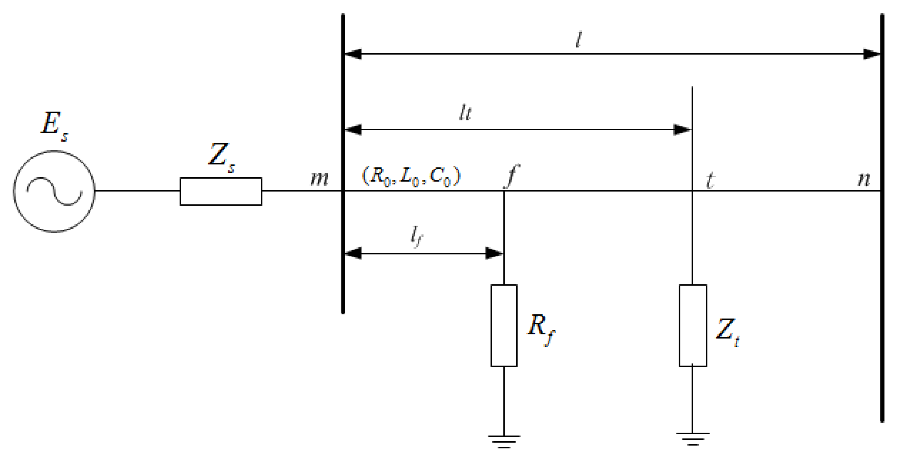
Generally, locomotion can be regarded as a direct current source (the empty load is infinitive) or a certain impedance, $Z_t$. The system is powered by one substation with the power source, $E_s$, and impedance, $Z_s$. Here, the locomotion is considered in the short-circuit ground-faulted model, which is the most general fault type in a traction line system, as shown in Figure 1. m and n are the beginning point and terminal point of the traction line with length, l, where $l_f$ is the distance from m to the fault point, f, with transient resistance, $R_f$. The equivalent impedance at the measurement end is discussed with and without the locomotive load consideration. More complicated nonlinear resistor issues have never been answered for fault location in power traction systems. Because the resistor of power transmission lines is varied according to the type, size, duration and wear degree of the line, there is no precise formula for the complicated nonlinear resistor. Usually, the resistor of the power transmission line can be calculated by lumped parameters and the distribution parameters of the system [18]. Here, the complicated nonlinear resistor issue is not considered.

Figure 1. The equivalent model of the faulted traction system.

Figure 1. The equivalent model of the faulted traction system.

The energy transferring in the traction network system is analyzed via the transmission line equation [19]. Assuming the electrical traction line parameters are uniformly distributed, where the per-unit-length resistance, inductance and capacitance are, i.e., $R_0$, $L_0$, $C_0$, respectively. The ground inductance, $G_0$, is ignored, and the values of the parameters are listed in Table 1 [20]. The propagation constant, γ, and the characteristic impedance, $Z_c$, of the system parameters are:

$$\begin{array}{c}\hfill \begin{array}{c}\gamma =\sqrt{(R_0+jw{L}_0)jw{C}_0},Z_c=\sqrt{(R_0+jw{L}_0)/jw{C}_0}\end{array}\end{array}$$

(1)

where w is the angular frequency of the system. Firstly, the locomotion is not considered in the system. The equivalent impedance at the fault point f is:

$$Z_{fn}=\frac{R_f{Z}_{c}coth\left[\gamma (l-l_f)\right]}{R_f+Z_{c}coth\left[\gamma (l-l_f)\right]}$$

(2)

Table 1. The parameters of the electrical line.

Parameter		Value
$R_0$	(Ω/km)	0.1–0.3
$L_0$	(mH/km)	1.4–2.3
$C_0$	(nF/km)	10–14

Table 1. The parameters of the electrical line.

Parameter		Value
$R_0$	(Ω/km)	0.1–0.3
$L_0$	(mH/km)	1.4–2.3
$C_0$	(nF/km)	10–14

Then, the equivalent impedance at the m-end to the line terminal is:

$$Z_{mn}=\frac{Z_{fn}cosh\left(\gamma l_f\right)+Z_{c}sinh\left(\gamma l_f\right)}{Z_{fn}sinh\left(\gamma l_f\right)/Z_c+cosh\left(\gamma l_f\right)}=f(w,l_f)$$

(3)

In the next step, the locomotion is considered in the faulted model. If the locomotive is between the substation and fault position, i.e., $l_t<l_f$, then the impedance at the fault point, f, is:

$$Z_{fn}=\frac{R_f{Z}_{c}coth\left[\gamma (l-l_f)\right]}{R_f+Z_{c}coth\left[\gamma (l-l_f)\right]}$$

(4)

Thus, the equivalent impedance at the locomotive position, t, is:

$$Z_{tn}=\frac{Z_{tnl}{Z}_t}{Z_{tnl}+Z_t}$$

(5)

where $Z_{tnl}=\frac{Z_{fn}cosh\left(\gamma (l_f-l_t)\right)+Z_{c}sinh\left(\gamma (l_f-l_t)\right)}{Z_{fn}sinh\left(\gamma (l_f-l_t)\right)/Z_c+cosh\left(\gamma (l_f-l_t)\right)}$. Hence, the impedance to the terminal at the m-end is:

$$Z_{mn}=\frac{Z_{tn}cosh\left(\gamma l_t\right)+Z_{c}sinh\left(\gamma l_t\right)}{Z_{tn}sinh\left(\gamma l_t\right)/Z_c+cosh\left(\gamma l_t\right)}$$

(6)

If the locomotive is between the fault position and the line terminal, i.e., $l_t>l_f$, then the impedance at locomotive position, t, is:

$$Z_{tn}=\frac{Z_t{Z}_{c}coth\left[\gamma (l-l_t)\right]}{Z_t+Z_{c}coth\left[\gamma (l-l_t)\right]}$$

(7)

The impedance at the f position is $Z_{fn}=\frac{Z_{fnl}{R}_f}{Z_{fnl}+R_f}$, where $Z_{fnl}=\frac{Z_{tn}cosh\left(\gamma (l_t-l_f)\right)+Z_{c}sinh\left(\gamma (l_t-l_f)\right)}{Z_{tn}sinh\left(\gamma (l_t-l_f)\right)/Z_c+cosh\left(\gamma (l_t-l_f)\right)}$. Therefore, the impedance at the m-end to the line terminal is:

$$Z_{mn}=\frac{Z_{fn}cosh\left(\gamma l_f\right)+Z_{c}sinh\left(\gamma l_f\right)}{Z_{fn}sinh\left(\gamma l_f\right)/Z_c+cosh\left(\gamma l_f\right)}=f(w,l_f)$$

(8)

It can be seen that $Z_{mn}$ is the function of angular frequency, w, with electrical traction line parameters. The frequencies, $f_{res}$, are the first to third harmonic frequency points of the harmonic frequencies $(w=2\pi \times f_{res})$. Through the analysis of the relationship between the equivalent impedance and fault location in the faulted system, from the frequency perspective, the fault distance can be obtained accordingly. The detailed algorithm will be described in the next section.

3. The Algorithm of Fault Location Based on Fault High-Frequency Transient Characteristics

3.1. The Relationship between the Harmonic Frequency, $f_{res}$, and Fault Distance, $l_f$

To obtain exact harmonic frequencies, $f_{res}$, a partial derivative equation can be used for exact calculation from Equations (6) and (8). Since there are a lot of parameters in the equivalent impedance, $Z_{mn}$, the deduction is very complicated, and simulation experiments are used instead without loss of generality.

According to the range of line parameters shown in Table 1, here, we select $R_0=0.232\mathsf{\Omega }/km$, $L_0=1.64mH/km$, $C_0=10.5nF/km$, and the length of transmission line, l, is 30 km, $R_f=0\mathsf{\Omega }$. When the locomotive position is $l_t=19km$ and a fault happens at positions, i.e.,

$$l_f=[12km,24km]$$

(9)

the relationship between the magnitude of the impedance, $Z_{mn}$, and the frequencies based on the calculation in Equations (6) and (8) are shown in Figure 2.

Figure 2. The amplitude of $Z_{mn}$ versus frequency with different $l_f$.

Figure 2. The amplitude of $Z_{mn}$ versus frequency with different $l_f$.

Apparently, the harmonic frequencies will change with the variation of fault positions. Through a lot of digital simulation experiments, it demonstrates that $l_f$ and harmonic frequencies, $f_{res}$, have a nonlinear relationship between them. The curves of the first three harmonic frequency points and the fault distances are depicted in Figure 3. In that case, if the harmonic frequency values have been found, the fault distance can be determined accordingly. The accuracy of the obtained fault distance is dependent on the precision of the relationship curve. The more data selected in the curve, the more accurate is the obtained fault distance estimation.

Figure 3. The relationship between the harmonic frequencies and fault points.

Figure 3. The relationship between the harmonic frequencies and fault points.

3.2. Theory of Fault Distance Measurement Based on Fault Transient Behavior

At the occurrence of a fault in the traction network, the spectrum of the transient response of the current and voltage are continuous under the motivation of the fault voltage component [21]. Thus, based on the circuit principle, any frequency, along with the line, has the following formulas:

$${\dot{U}}_m={\dot{I}}_m{Z}_{mn}$$

(10a)

$${\dot{E}}_s={\dot{U}}_m+{\dot{I}}_m{Z}_s$$

(10b)

where ${\dot{U}}_m$ and ${\dot{I}}_m$ are the voltage and current at the measurement point, m; ${\dot{E}}_s$ and $Z_s$ are the power source and impedance. $E_s$ is the magnitude of the power source. ${\dot{U}}_m$ and ${\dot{I}}_m$ share the same harmonic frequency points, since they share the same denominator, which are both deduced from Equation (10a,b).

In order to analyze the frequency characteristics of the transient voltages or current signals at the measurement end in the high frequency region, the influence of low-frequency, especially the fundamental frequency components of the signals, must be removed. Moreover, when a fault happens in the proximal area, it is easily affected by the cut-off frequency. Therefore, the transient voltage signal is chosen to be the input data for distance measurement. Referring to [22], an oval high-pass filter is selected with a cut-off frequency of 4.2 kHz. After filtering the low-frequency signals, fast Fourier transform (FFT) is adopted for the dealt signal, then the high-frequency spectrum curve is obtained.

When the locomotive position, $l_t$, is 10 km, the fault position, $l_f$, is 19 km, the transient resistance, $R_f$, is 100 Ω and system sampling frequency is 500 kHz, then the frequency curve of $Z_{mn}$ is depicted in Figure 4. The frequency spectrums of the transient voltage and current signals after removing the disturbance at low frequencies via high-pass filters and fast Fourier transformation (FFT) are shown in Figure 4b,c.

Figure 4. The frequency spectrum of the faulted traction network system. (a) the frequency spectrum of $Z_{mn}$; (b) the frequency spectrum of the filtered transient voltage signal; and (c) the frequency spectrum of the filtered transient current signal.

Figure 4. The frequency spectrum of the faulted traction network system. (a) the frequency spectrum of $Z_{mn}$; (b) the frequency spectrum of the filtered transient voltage signal; and (c) the frequency spectrum of the filtered transient current signal.

Hence, the extreme points of the measured electrical signals during fault dynamics can be found after filtering low-frequency components via the analysis of its spectrum at the high-frequency region. The frequency, $f_{res}$, is related to the fault distance. Figure 5 shows the relationship between fault distances and the first three extreme values of the measurement voltage spectrum, ${\dot{U}}_m$, at its high-frequency region. The experiments are running under different situations: fault distances (from 1–29 km, step size is 1 km), and different fault transition resistance (0, 50, 100) Ω. Comparing Figure 5 with Figure 3, this demonstrates that the curves follow the same changing pattern, which verifies further the corresponding relationship between the extreme points of the transient component spectrum of the harmonic frequencies of ${\dot{U}}_m$ and the fault distances. Via the analysis of characteristics of the harmonic frequencies of ${\dot{U}}_m$ in the high-frequency domain, the fault location can be obtained.

Figure 5. The harmonic frequency curves of ${\dot{U}}_m$ versus fault distances.

Figure 5. The harmonic frequency curves of ${\dot{U}}_m$ versus fault distances.

3.3. The Algorithm of the Fault Distance Estimation

The fault distance estimation can be derived from the relationship curve of harmonic points of ${\dot{U}}_m$ and fault distance, where the step of the fault distance is 1 km. Figure 5 includes three curves, and each curve consists of many points, which are the related fault locations per 1000 m. It can be seen from Figure 5 that the curve is quite flat when a fault occurs at the far end (away from the electrical substation), which means that the fault distance discrimination ratio is decreased and the harmonic frequencies, $f_{res}$, are insensitive to the fault distance. The sampling frequency is 500 kHz. The maximum frequency is $2.5\times {10}^5$ Hz, as shown in Figure 4b,c, since the frequency spectrum is Fourier transformed symmetrically. The first half of the picture is the same as the second half, so the second half is omitted. When a fault occurs close to the substation, $f_{res}$ is too sensitive to the fault distance. Specially, a small fluctuation of the frequency would result in a large fault distance difference.

In Figure 5, the $1st$ frequency spectrum extreme point curve has good discrimination to the fault distance variation when it is close to the end of the traction line, but it is too sensitive at the beginning and middle of the line. The $2nd$ frequency curve is too sensitive at the beginning of the line, with good precision in the middle of the line and low precision at the end of the line. Moreover, the $3rd$ frequency curve has better discrimination at the beginning of the line, but low precision at the middle and end of the line. With the consideration of stability, discrimination ratio and signal sampling frequency, piece-wise segments of the curves should be selected to represent the relationship between the harmonic frequency points and fault distances accurately.

Due to the complex test conditions and field operational environments, the test results could be compromised, because of over sensitivity to the distance variation and low discrimination ratio. Considering the constraints on stability, discrimination and signal sampling frequency in the measurement system, the curve related to the $3rd$ extreme point frequency spectrum should be taken at the beginning period of the line. The curve related to the $2nd$ extreme points should be taken in the middle of the line. The $1st$ extreme point curve is adopted for the fault distance description at the end of the line.

In MATLAB simulation environment, through curve-fitting approaches, the three curve functions can be obtained. The first curve function is:

$$l_f=-0.0002\times f_e^3+0.0275\times f_e^2-0.9968\times f_e^1+13.6760$$

(11)

The second curve function is:

$$l_f=-0.0011f_e^3+0.094f_e^2-2.878f_e^1+37.9538$$

(12)

The third curve function is:

$$l_f=-0.0056f_e^3+0.3522f_e^2-8.1302f_e^1+81.7711$$

(13)

Combining these three curves, more accurate fault distance curves versus high-frequency spectrum extreme points can be derived, which is shown in Figure 6. This can be used for precise fault location. Simulation experiments will be performed to prove the accuracy of the obtained fault location from the relationship curve of the fault distance and harmonic extreme points of the system.

Figure 6. The harmonic frequency curves of $f_{res}$ versus fault distance, $l_f$.

Figure 6. The harmonic frequency curves of $f_{res}$ versus fault distance, $l_f$.

4. The Analysis of the Fault Location Algorithm

In this section, the factors related to the fault location algorithm are discussed. The calculated fault distance can be evaluated compared to the actual fault distance with the aid of the error equation:

$$e_{l_f}=\left|\frac{{\widehat{l}}_f-l_f}{l}\right|\times 100\%$$

(14)

where ${\widehat{l}}_f$ is the calculated fault distance from the developed algorithms and $l_f$ is the actual fault point in the system; $|·|$ is the calculated absolute value.

4.1. The Influence of Locomotion on the Fault Location Algorithm

In Section 2, the equivalent impedance, $Z_{mn}$, at the measurement m-end is discussed in two conditions. Hence, the influence of locomotion, i.e., position and load, to the $f_{res}$ of ${\dot{U}}_m$ should be discussed.

The zero-voltage protection method is adopted in the traction network. When the voltage of the locomotive decreases to zero or close to zero in $1s$ period, the protection is activated to cut off the operation. In this method, the voltage is used at the fault occurrence after one industrial-frequency period. The locomotive is still running during this time period. Hence, the influence of the position and load of the locomotive has to be considered in the algorithm.

Table 2 lists the calculated fault distance results with various locomotive positions when $l_f=19km$, $R_f=50\mathsf{\Omega }$ and $Z_t=60+80j$. This demonstrates that the locomotive location has quite a small impact on the fault distance location with an error of 0.5%. When the locomotive is close to the measurement terminal, the measurement error will be smaller, due to the decreased inductance in the line and the less decreased error in the fitting curves.

Table 3 lists the calculated fault distances under different various locomotive loads. When the locomotive load and fault points vary at the same time, the measurement error is still small, less than 0.9%. However, if the fault point is near the beginning end and terminal end of the line, the measurement error will be larger with the larger locomotive load. If the fault occurs in the middle parts of the line, the variation of the locomotive load will have less effect on the fault distance measurement. This demonstrates that the locomotive has little effect on the $f_{res}$ of the voltage of ${\dot{U}}_m$ and the fault location algorithm.

Table 2. The influence of locomotive position on the algorithm.

$l_f$	Locomotive position $l_t$
	2	5	8	14	17	20	23	28
${\widehat{l}}_f$	18.9135	18.8557	18.9135	18.8557	18.8557	18.8557	18.8557	18.8557
$e_{l_f}$	0.2883	0.2883	0.4810	0.4810	0.4810	0.4810	0.4810	0.4810

Table 2. The influence of locomotive position on the algorithm.

$l_f$	Locomotive position $l_t$
	2	5	8	14	17	20	23	28
${\widehat{l}}_f$	18.9135	18.8557	18.9135	18.8557	18.8557	18.8557	18.8557	18.8557
$e_{l_f}$	0.2883	0.2883	0.4810	0.4810	0.4810	0.4810	0.4810	0.4810

Table 3. The influence of locomotive load on the algorithm.

$Z_t$	$l_f$	Calculated $l_f$	$e_{l_f}$
$Z_t$ = 54 + 72j	2	2.05817	0.1939
	5	5.21508	0.7169
	14	14.0090	0.0300
	17	17.0619	0.2063
	28	27.9911	0.0297
$Z_t$ = 60 + 80j	2	2.18081	0.6027
	5	5.21508	0.7169
	14	14.0090	0.0300
	17	17.1539	0.5130
	28	27.9911	0.0297
$Z_t=\infty$	2	2.18081	0.6027
	5	5.21508	0.7169
	14	14.0090	0.0300
	17	17.0619	0.2063
	28	27.7446	0.8513

Table 3. The influence of locomotive load on the algorithm.

$Z_t$	$l_f$	Calculated $l_f$	$e_{l_f}$
$Z_t$ = 54 + 72j	2	2.05817	0.1939
	5	5.21508	0.7169
	14	14.0090	0.0300
	17	17.0619	0.2063
	28	27.9911	0.0297
$Z_t$ = 60 + 80j	2	2.18081	0.6027
	5	5.21508	0.7169
	14	14.0090	0.0300
	17	17.1539	0.5130
	28	27.9911	0.0297
$Z_t=\infty$	2	2.18081	0.6027
	5	5.21508	0.7169
	14	14.0090	0.0300
	17	17.0619	0.2063
	28	27.7446	0.8513

4.2. The Influence of Transient Resistance, $R_f$, to the Fault Location Algorithm

Since the transient resistance, $R_f$, will change randomly at the occurrence of a fault, its influence has to be discussed. The experiments are performed under different transient resistances,

$$R_f=[0,50,100]\mathsf{\Omega }$$

(15)

when the fault position is at $l_f=19km$, $Z_t=60+80j$. The error of the calculated fault distances and actual fault distances is depicted in Figure 7. Considered the effect of less sampling points and the accuracy of the fitting curves, the lines appear a little bit disordered. We can still obtain the changing pattern of the measurement error becoming larger when the transient resistance is larger under the condition of the same fault location. During practical operation, faults always display the characteristics of transit resistance contacting the ground, which is one of the key research topics for the resistance distance measurement method. For solving the problem, additional assistant approaches have been sought to remove the influence of transient resistance, i.e., reactance, over-zero detection, which can improve the precision of fault distance estimation to a certain degree. However, this cannot fully satisfy the requirement of on-site operational requirement. With the application of the proposed algorithm, the measurement errors in the experiments are almost less than 1%. This suggests that there is only a small error in the algorithm of the fault position measurement, due to offset in the harmonic frequency points. Although the offsets are different in each harmonic frequency point, they are kept in a small range, which can be ignored. Therefore, the fault transient resistance, $R_f$, has little effect on the proposed fault location algorithm.

Figure 7. The influence of $R_f$ on the algorithm.

Figure 7. The influence of $R_f$ on the algorithm.

4.3. The Influence of Transmission Line Parameters on the Fault Location Algorithm

Many factors could cause instability for the per-unit-length line parameters. The locomotive obtaining the current from the panograph slider would wear down the wire gradually. Besides, the replacement of the wire in a certain region and frequently manual examination of the wire could also cause variation in line parameters. The obtained fault results from the fault location algorithm under different line parameters,

$$Z_l=[Z_{l1},Z_{l2},Z_{l3}],$$

(16)

$$\begin{array}{cc}\mathrm{where},& Z_{l1}=[R_0=0.23\mathsf{\Omega },L_0=1.64mH,C_0=10.5nF]/km\\ & Z_{l2}=[R_0=0.23\mathsf{\Omega },L_0=2.3mH,C_0=10.5nF]/km\\ & Z_{l3}=[R_0=0.23\mathsf{\Omega },L_0=1.64mH,C_0=11.06nF]/km\end{array}$$

when the locomotive is $Z_t=60+j80$, $l_t=19km$ and $R_f=50\mathsf{\Omega }$, as described in Figure 8. This shows that the resistance, $R_0$, of the line parameter has little impact on the proposed algorithm. However, the inductance and capacitance of the parameters, $L_0$ and $C_0$, do have a certain effect on the results of the calculated fault location. When the inductance in the line resistance varies, the measurement errors will raise, accompanied by the fault distance increment, with a maximum error of $15\%$, which has much of an effect on the fault location estimation. The main reason is that the inductance can quickly restrain varied voltage and current in the line. When the capacitor in the line changes, the measurement error will also grow bigger if the fault distance becomes larger, with a maximum error of 3%. Compared to the results, inductance has more of an effect on the measurement error of the fault location than that of the capacitor. Therefore, the variation of the line condition, such as aging, should be kept in close observation, so as to reduce its influence in the fault location algorithm.

Figure 8. The influence of $Z_l$ on the algorithm.

Figure 8. The influence of $Z_l$ on the algorithm.

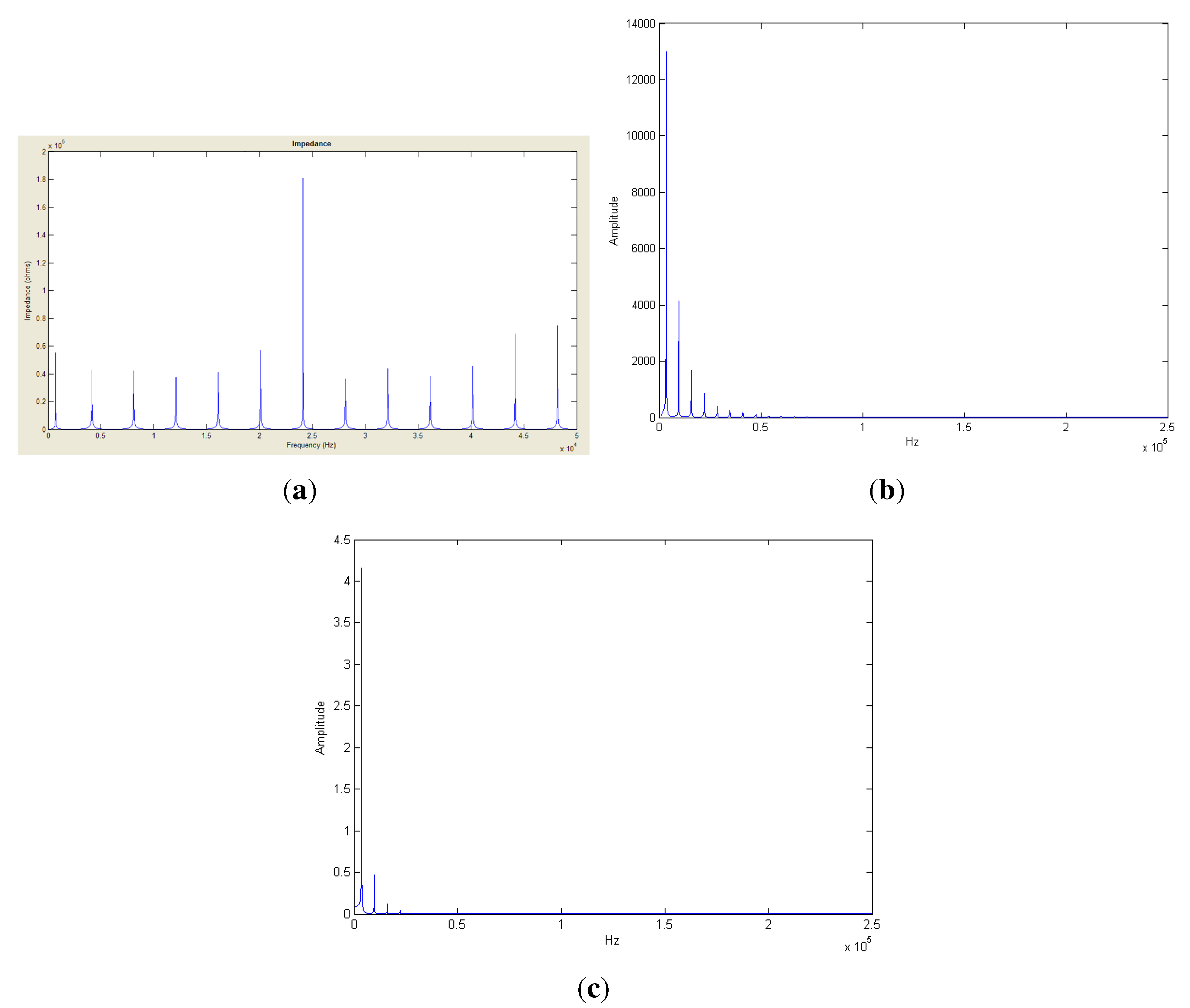
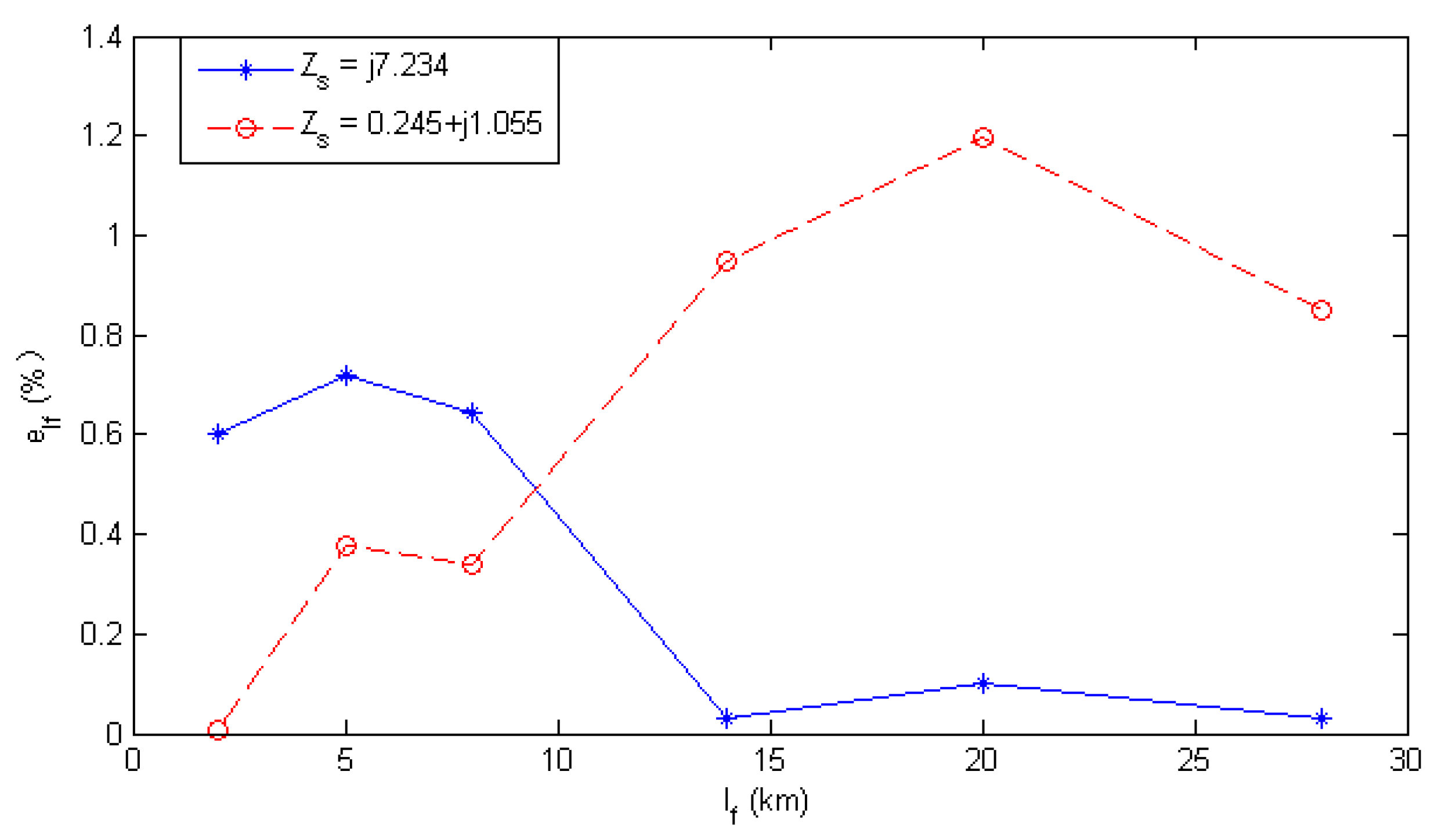
4.4. The Influence of $Z_s$ to $f_{res}$

A three-phase traction substation normally has two three-phase YN, d11 (connection form) traction transformer, which can be used in parallel at the same time, or one put in use and the other as backup. Besides, the external characteristics of the traction substation will be affected, because of the neighboring electric arm load current. The amplitude of the $Z_{mn}$ versus different frequencies is shown in Figure 4. It can be seen that the magnitude of $Z_s$ is too small compared to $Z_{mn}$. Here, the calculated fault distances under different impedances of the power source,

$$Z_s=[0.245+j1.055,j7.243]\mathsf{\Omega }$$

(17)

when the locomotive is $Z_t=60+j80$, $l_t=19km$ and $R_f=50\mathsf{\Omega }$ are described in Figure 9.

Figure 9. The influence of $Z_s$ on the algorithm.

Figure 9. The influence of $Z_s$ on the algorithm.

As mentioned earlier, the equivalent system resistance will be changed to a certain degree during operation. Therefore, the system resistance variation will be $\pm 50\%$. When the internal resistance, $Z_s$, in the power source changes, the inductance of $Z_s$ will affect the voltage frequency at the measurement end. Besides, the accuracy of the fault location fitting curves will bring some measurement error. In practical applications, to guarantee the accuracy of the fault distance measurement, the system resistance, $Z_s$, can be measured online based on the voltage and current at the measurement terminal to obtain the harmonic frequency points with high accuracy.

5. Simulation Results

As for the fault distance location algorithm, the most evaluation criteria should include at least two items. One is the robustness, i.e., it can provide accurate measurement results in any faulty situations with a broad applicable scope. The other is the precision, i.e., the difference between the measured fault distance and the actual fault distance. Without enough precision, this means the failure of the fault location. During on-site operation, the precision of the distance location algorithm will be affected by many factors, such as sampling channel, CT (Current Transformer) and PT (Power Transformer) error. Here, we will only analyze the algorithm theoretically and omit the disturbance from data collection and sensor errors.

The traction power supply system is quite an independent and special branch in the power system; therefore, each fault distance measurement algorithm has its own applicable conditions. The proposed algorithm is based on single-end measurement theory, which is easily affected by the system operational method, fault occurrence angle, transient resistance, the locomotive and transmission line parameter variation factors. Reliability is a qualitative concept, and it is difficult to be quantified. Robustness is then introduced to analyze the reliability quantitatively. As for the robustness in the fault distance measurement algorithm, the boundary for all kinds of disturbances is sought. The algorithm will be more robust with larger boundary values. Here, the robustness is defined as: the absolute error of the fault distance measurement will be less than $1km$ under certain disturbance circumstances.

In the following experiments, single-phase industrial-frequency AC power is supplied for the electrical traction system described in Figure 1. Normally, the electrical substation transforms the three-phase 110 kV high voltage into 27.5 kV voltage and the impedance, $Z_s=0.245+j1.055$, and assigns the single-phase to each traction system. MATLAB simulation tool is used for the experiments. The time for the fault occurring is $0.065s$, and the signal collection time is 0–$1.4s$; the sampling frequency is $200kHz$. The voltage at the measurement end is filtered by the oval high-pass filter and FFT calculation. Fault distance can be calculated from Equations (3), (6) and (8).

Transient resistance is the uppermost factor to influence the single-end fault distance measurement. Considering the empty load and with load circumstances, the simulation experiments are performed when the fault happens at the near end ($2km$), middle part ($6.5km$, $17km$) and far end ($27km$). Table 4 and Table 5 list the calculated fault distance results with the proposed algorithm and with the reactance method, where error, $e_{l_f}$, is calculated from Equation (14) for comparison. This indicates that the proposed algorithm has higher robustness.

The fault location results are shown in Table 6 under different transmission line parameters with $R_f=50\mathsf{\Omega }$ and $l_t=19km$. It can be demonstrated that the proposed algorithm for fault location is not disturbed by the fault transient resistance and the locomotive position. This possesses high precision and robustness for fault distance measurement.

Table 4. The $l_f$ calculation when the locomotive load, $Z_t=\infty$, is empty.

Transient resistance $R_f\left(\mathsf{\Omega }\right)$	Fault distance $l_f\left(\mathrm{km}\right)$	Fault distance measurement and results
		Reactance		New algorithm
		${\widehat{l}}_f$	$e_{l_f}$ (%)	${\widehat{l}}_f$	$e_{l_f}$ (%)
0	2	1.9896	0.0347	2.0352	0.1173
	6.5	6.4665	0.1117	6.5416	0.1387
	17	16.9142	0.2860	17.0987	0.3290
	27	26.8690	0.4367	26.9783	0.0723
50	2	1.5114	1.6287	2.0352	0.1173
	6.5	6.4665	1.7157	6.5416	0.1387
	17	16.9142	1.9567	17.0987	0.3290
	27	26.8690	2.2233	26.9783	0.0723
100	2	0.0776	6.4080	2.0352	0.1173
	6.5	4.5486	6.5047	6.5416	0.1387
	17	14.957	6.8100	17.0987	0.3290
	27	24.8414	7.1953	26.9783	0.0723

Table 4. The $l_f$ calculation when the locomotive load, $Z_t=\infty$, is empty.

Transient resistance $R_f\left(\mathsf{\Omega }\right)$	Fault distance $l_f\left(\mathrm{km}\right)$	Fault distance measurement and results
		Reactance		New algorithm
		${\widehat{l}}_f$	$e_{l_f}$ (%)	${\widehat{l}}_f$	$e_{l_f}$ (%)
0	2	1.9896	0.0347	2.0352	0.1173
	6.5	6.4665	0.1117	6.5416	0.1387
	17	16.9142	0.2860	17.0987	0.3290
	27	26.8690	0.4367	26.9783	0.0723
50	2	1.5114	1.6287	2.0352	0.1173
	6.5	6.4665	1.7157	6.5416	0.1387
	17	16.9142	1.9567	17.0987	0.3290
	27	26.8690	2.2233	26.9783	0.0723
100	2	0.0776	6.4080	2.0352	0.1173
	6.5	4.5486	6.5047	6.5416	0.1387
	17	14.957	6.8100	17.0987	0.3290
	27	24.8414	7.1953	26.9783	0.0723

Table 5. The $l_f$ calculation when the locomotive load is $Z_t=60+j80$, $l_t=25km$.

Transient resistance $R_f\left(\mathsf{\Omega }\right)$	Fault distance $l_f\left(\mathrm{km}\right)$	Fault distance measurement and results
		Reactance		New algorithm
		${\widehat{l}}_f$	$e_{l_f}$ (%)	${\widehat{l}}_f$	$e_{l_f}$ (%)
0	2	1.9896	0.0343	2.04095	0.1365
	6.5	6.4665	0.1120	6.5424	0.1413
	17	16.9142	0.2860	17.0803	0.2677
	27	26.8690	0.4487	17.0803	0.0410
50	2	10.4783	28.2610	2.05817	0.1939
	6.5	14.9939	28.3130	6.61506	0.3835
	17	25.5263	28.4210	17.34134	1.1378
	27	35.6100	28.7000	27.02523	0.0841
100	2	34.3920	107.9733	2.18081	0.6027
	6.5	39.01992	108.3997	6.56416	0.2139
	17	49.82117	109.4039	17.1539	0.5130
	27	60.0829	110.2763	26.7920	0.6933

Table 5. The $l_f$ calculation when the locomotive load is $Z_t=60+j80$, $l_t=25km$.

Transient resistance $R_f\left(\mathsf{\Omega }\right)$	Fault distance $l_f\left(\mathrm{km}\right)$	Fault distance measurement and results
		Reactance		New algorithm
		${\widehat{l}}_f$	$e_{l_f}$ (%)	${\widehat{l}}_f$	$e_{l_f}$ (%)
0	2	1.9896	0.0343	2.04095	0.1365
	6.5	6.4665	0.1120	6.5424	0.1413
	17	16.9142	0.2860	17.0803	0.2677
	27	26.8690	0.4487	17.0803	0.0410
50	2	10.4783	28.2610	2.05817	0.1939
	6.5	14.9939	28.3130	6.61506	0.3835
	17	25.5263	28.4210	17.34134	1.1378
	27	35.6100	28.7000	27.02523	0.0841
100	2	34.3920	107.9733	2.18081	0.6027
	6.5	39.01992	108.3997	6.56416	0.2139
	17	49.82117	109.4039	17.1539	0.5130
	27	60.0829	110.2763	26.7920	0.6933

Table 6. The $l_f$ calculation with different line parameters.

Condition	Line Paramater $Z_L$	Fault distance $l_f\left(\mathrm{km}\right)$	Fault distance measurement and results
			Reactance		New algorithm
			${\widehat{l}}_f$	$e_{l_f}$ (%)	${\widehat{l}}_f$	$e_{l_f}$ (%)
$R_f=50\mathsf{\Omega }$ $l_t=19km$	ZL1	2	10.5385	28.4617	2.18081	0.6027
		6.5	15.0544	28.5147	6.7178	0.7260
		17	25.5882	28.6273	17.1539	0.5130
		27	35.7536	29.1787	26.192	2.6933
	ZL2	2	11.2869	30.9563	2.39742	1.3247
		6.5	17.6178	37.0593	7.6579	3.8597
		17	32.3921	51.3070	20.1630	10.5433
		27	46.3592	64.5307	31.519	15.0633
	ZL3	2	10.5148	28.3827	2.18081	0.6027
		6.5	15.0304	28.4347	6.8316	1.1053
		17	25.5632	28.5440	17.5333	1.7777
		27	35.7284	29.0947	27.5015	1.6717

Table 6. The $l_f$ calculation with different line parameters.

Condition	Line Paramater $Z_L$	Fault distance $l_f\left(\mathrm{km}\right)$	Fault distance measurement and results
			Reactance		New algorithm
			${\widehat{l}}_f$	$e_{l_f}$ (%)	${\widehat{l}}_f$	$e_{l_f}$ (%)
$R_f=50\mathsf{\Omega }$ $l_t=19km$	ZL1	2	10.5385	28.4617	2.18081	0.6027
		6.5	15.0544	28.5147	6.7178	0.7260
		17	25.5882	28.6273	17.1539	0.5130
		27	35.7536	29.1787	26.192	2.6933
	ZL2	2	11.2869	30.9563	2.39742	1.3247
		6.5	17.6178	37.0593	7.6579	3.8597
		17	32.3921	51.3070	20.1630	10.5433
		27	46.3592	64.5307	31.519	15.0633
	ZL3	2	10.5148	28.3827	2.18081	0.6027
		6.5	15.0304	28.4347	6.8316	1.1053
		17	25.5632	28.5440	17.5333	1.7777
		27	35.7284	29.0947	27.5015	1.6717

After the short-circuit fault occurs in the traction network, it generates the static and transient two fault components, which have redundant information. The fault distance measurement method in [3] is based on the static fault information for the fault distance calculation. The used industrial frequency static vector is quite stable and reliable, but the algorithm is more complicated, especially for the amplitude and phase extraction, which has relatively low precision. The proposed algorithm in this paper adopts the high-frequency component of the fault transient voltage to measure the fault distance. The involved theory is simple and has little effect on the locomotive, transient resistance factors. It possesses high precision, but is easily affected by variation of the system resistance. With the combination of the two algorithms mentioned in [3] and in this paper, this will greatly improve the performance of the fault distance measurement with high precision and robustness via appropriate information fusion technology.

It is worthy noting that the technique in this paper is not mature and lacks practical operation experience. Besides, due to the transient signal adopted for fault location, disturbance signals would be introduced. The high precision and high sampling frequency voltage sensors are required, as well. In summary, however, the developed fault distance measurement algorithms in a power traction system supplied by one electrical supply substation has the following features:

(1)

The fault location can be estimated with only the voltage at the measurement end;

(2)

The results are not influenced by the load flow, position and transient fault resistance;

(3)

The results are not influenced by the supplied power source;

(4)

The results are not influenced by the variations of the transmission line parameters (stable condition).

This can be expanded to an AT (AutoTransformer) and BT (Booster Transformer) abbreviations power supply traction network, with bright industrial application prospects.

6. Conclusions

In this paper, a precise fault location algorithm is discussed based on the fault transient frequency characteristics. The fault distance can be obtained in the high frequency domain with only the knowledge of voltages and currents at the measurement terminal of the transmission line. Furthermore, it investigates the factors of transient resistance, locomotion and fluctuation in electrical line parameters to the proposed algorithms. The results of the estimated fault location are quite accurate compared to the traditional methods. The proposed algorithm can be applied in the distance measurement of high voltage transmission lines in power traction systems. In the future, field experiments will be implemented to further prove the effectiveness of the proposed fault location algorithm.