Contribution of Small Wind Turbine Structural Vibration to Noise Emission

Abstract

A major barrier to the acceptance of small wind turbines is that they are perceived to be noisy. This paper investigates an aspect of noise emission that has not been considered; vibration and noise generation from the tower. First, vibration measurements were made using accelerometers placed on the 10.2 m monopole tower of a Skystream 2.4 kW wind turbine, and natural frequencies and corresponding deflection shapes were calculated. Second, the results from the survey were used to verify the predictions of a finite element model of the tower structure. Lastly, the tower’s acoustic emission was simulated computationally, as it was not possible to measure it accurately. Most vibration energy occurred in the very low frequency band (≤10 Hz). It was found that wind itself can only excite the first two bending modes. On the other hand, emitted noise from the tower at large distances can be neglected, as close to the tower, the noise can reach 30 dB.

1. Introduction

Wind turbines generate electricity in a wide variety of sizes. Large wind turbines are usually installed in wind farms, producing large amounts of electricity. Small wind turbines (SWTs) on the other hand, which are defined according to the International Electrotechnical Commission (IEC), IEC 61400-2 [1], as having a swept area of less than 200 m${}^2$, correspond to a rated power of less than about 50 kW. They often supply single homes, farms and small businesses and may also be part of hybrid remote power systems. According to the American Wind Energy Association (AWEA) [2], the installed capacity increased by 78% in 2008. This growth has brought significant interest in SWTs for urban usage.

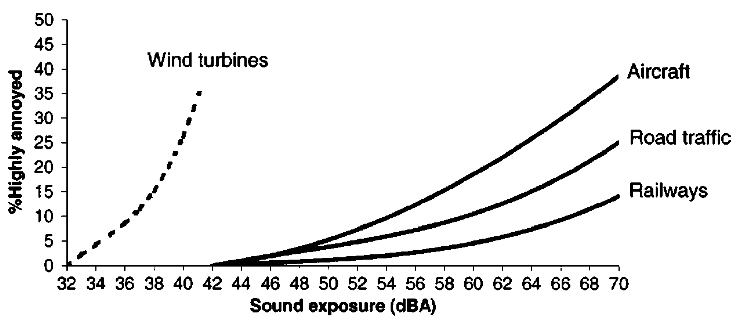
1.1. Small Wind Turbine Noise Perception

There are many considerations of wind assessment, noise and visual impact in the site determination for large wind turbines. SWTs, however, are usually located close to the load they supply, which means they are usually much closer to residences, which increases their potential for noise pollution. It has been reported that wind turbines produce very little noise. Lawson’s [3] early data correlation indicated that the sound power level of a wind turbine is approximately one-ten-millionth of the rated power. Still, people have different perceptions of noise, and many believe that turbines are noisy. For example, Pedersen et al. [4] investigated how wind turbines can annoy people; see Figure 1. Transportation noise, such as aircraft, road traffic and railways, are all perceived as noise at a higher sound pressure level compared to wind turbines. Sources of wind turbine noise have been classified into four categories: tonal, broadband, infrasound, low frequency and impulsive [5], which are described as follows:

• Tonal noise was common in older turbines, which operated at constant blade speed. This type of noise is now uncommon, as most turbines are variable frequency;
• Broadband noise has frequency components higher than 100 Hz. This is produced typically by the blade interaction with the wind turbulence, leading to swishing;
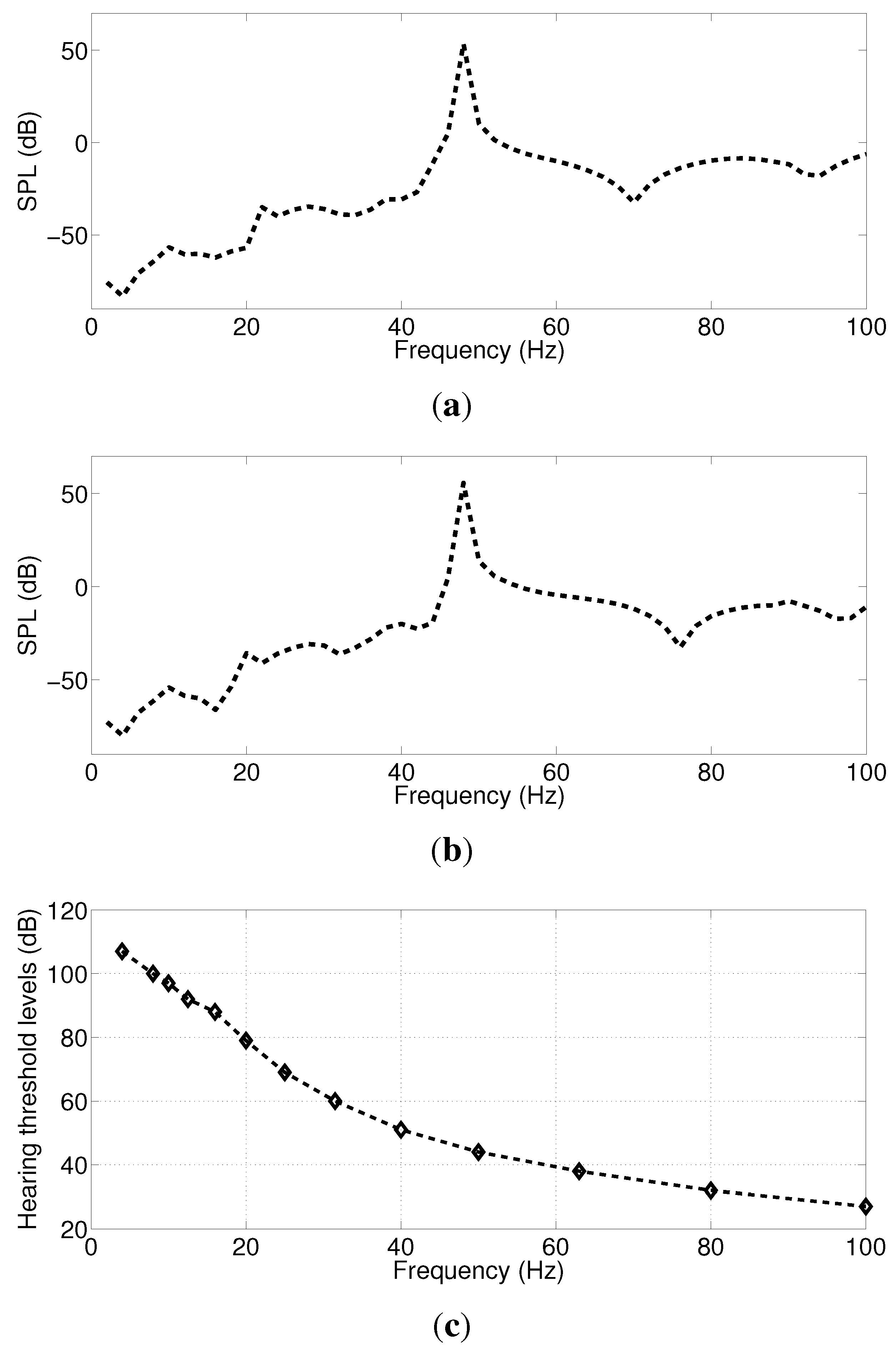
• Infrasound refers to frequencies below the hearing frequency threshold of about 20 Hz;
• The low frequency range between 20 and 100 Hz is suspected of irritation and includes contributions from blade-tower noise for downwind rotors, such as the one studied in this paper;
• Impulsive noise is the result of short acoustic impulses, whose amplitudes vary with respect to time. This is generated by the interaction of the blades with the disturbed air flow behind the tower of the downwind turbine.

Figure 1. Comparison between transportation noise and wind turbine noise annoyance [4].

Figure 1. Comparison between transportation noise and wind turbine noise annoyance [4].

Infrasound and low frequency noise can be amplified and, then, radiated by the tower surface. Tower vibrations originate from vibrations in the nacelle components and the blades passing the main shaft, as well as any potential eccentricities in the rotating parts. Even if the tower sound power level is small, the tower approximates a line source for a listener close to the turbine. Therefore, tower noise will be attenuated more slowly than the approximate “point source” noise from the rotor. Because of the small power outputs of SWTs, it is usually difficult to measure the noise of SWTs accurately in order to derive meaningful conclusions. It is even harder to decompose noise measurements into the many components. Instead, in this paper, tower vibration is studied to provide the basis to investigate the extent to which the tower contributes as a noise emitter.

This paper is organized as follows: Section 2 explains the vibration analysis using Operational Modal Analysis. The Frequency Domain Decomposition method is described and used to extract natural frequencies and deflection shapes. Section 3 describes the acoustic-structure interaction modelling and shows the importance of the wind turbine loads to the noise generation. Section 4 contains the conclusion.

2. Vibration Analysis

In order to study the dynamic properties of a system, modal analysis is used to determine modal parameters under dynamic excitation. The system could be a simple structure or a very complex model, including several subsystems. Basically, the response of a linear system to an excitation can be represented as a sum of the contributions from all the modes of the system.

Classical modal analyses are based on the measurements of both input force and output response. However, there are some limitations of Experimental Modal Analysis (EMA) that Operational Modal Analysis (OMA) can overcome:

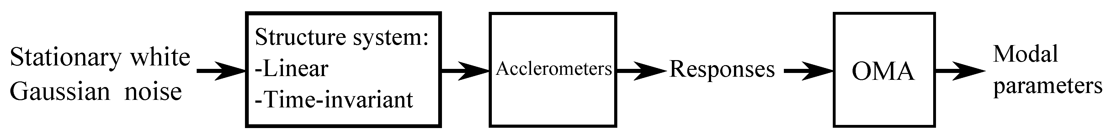
• Artificial excitation is usually conducted in the laboratory to determine the Frequency Response Function (FRF) and Impulse Response Function (IRF), which are mainly used as key data for corresponding modal parameter extraction. Input force and response may be very difficult to measure in the field for large structures, such as bridges and wind turbines. Furthermore, inputs, such as the wind and road vibration, are too complicated to characterize simply. Besides, a localized excitation could be insufficient to excite a large structure, and it is impossible to isolate such excitation from the environment excitation;
• In many applications, the actual modes may differ significantly from those measured in laboratory testing with artificial excitations. An SWT has many more noise sources while it is operating than when it is shut down. These include blade interaction with the tower and mechanical noise from the generator and other components. If the analyst is interested in vibration behaviour, rather than only modal parameters, then OMA would be more beneficial than EMA.

Rather, the modal experiment must be done in situ, with all the actual conditions, such as wind blowing, background noise etc. Although these conditions may pose some important challenges for EMA, OMA takes advantage of these factors by using them as the excitations and estimates the modal parameters. Therefore, both of the mentioned restrictions are addressed. More importantly, for this paper, OMA seeks to identify the vibration characteristics of the system while it is operating under the influence of presumably random, uncorrelated and broadband noise.

Figure 2 shows a schematic description of an ambient response system. OMA has come to considerable attention in the last two decades. It was developed in the 1970s, but researchers started applying it from the early 1990s [6]. Researchers in academia and engineers in industry have developed several methods to estimate modal parameters from measured data. Some approaches include peak-picking from Power Spectral Density (PSD) functions [7], Auto-Regressive Moving Average (ARMA) [8], subspace techniques [9] and the Natural Excitation Technique (NExT) by using cross-correlation functions instead of impulse response functions, which are coupled with time-domain schemes [10]. Among these different approaches, the Frequency Domain Decomposition (FDD) technique will be explained in Section 2.2, which uses the fact that modes can be estimated from spectral densities with the assumption of white noise input and a lightly dampened structure.

Figure 2. OMA model.

Figure 2. OMA model.

2.1. Literature Review

Although there are many applications of OMA to civil structures in the literature, such as [11], there are not many applications to wind turbines. James et al. [12] used NExT on a horizontal-axis wind turbine (HAWT) with the rotor diameter of 17.8 m. A successful modal extraction below 10 Hz was shown, including elastic vibration and blade rotation harmonics. Hansen et al. [13] performed OMA, along with an exciter mechanism, and showed limitations in terms of damping estimation, as the vibrations were not absolutely modal vibrations.

Tcherniak et al. [14] presented a successful and straightforward analysis on the 3 MW ECO 100 wind turbine tower using 12 accelerometers at five levels, yet found difficulty in identification of blade structural modes, due to the unavailability of acceleration data from them. They used Finite Element Modeling (FEM) to compare experimental and numerical results. Good agreement was reported, but there were still difficulties with identifying some modes, i.e., even to the extent of determining whether they were vertical or horizontal modes.

In another study, Chauhan et al. [15] investigated the time-varying nature of 3 MW wind turbine operation. Considerable aero-elastic effects along with harmonic components in the excitation were observed, which imposed limitations on the applicability of OMA. Multi-blade coordinate (MBC) transformation was shown to capture the rotor rotation frequency and its primary harmonics. MBC transformation converts the motion of individual blades in the rotating blade frame into the fixed frame, resulting in elimination of the time periodic terms present in the equations of motion and making application of OMA possible. However, the results were based on a conceptual turbine without any experiments. The authors also noted the differences in damping estimates between an eigenvalue solver and OMA, because the eigenvalue solver did not take aerodynamic forces into account and was based only on mass and stiffness, whereas damping varies, due to aerodynamic effects.

All these studies considered wind turbines ranging from 100 kW to 3 MW. No specific effort has been made on SWTs, except Styles et al. [16], who studied low-frequency vibration transmission from the tower to the ground. They used seismometers in different distances in order to study the vibration path and the interaction with other facilities kilometres away.

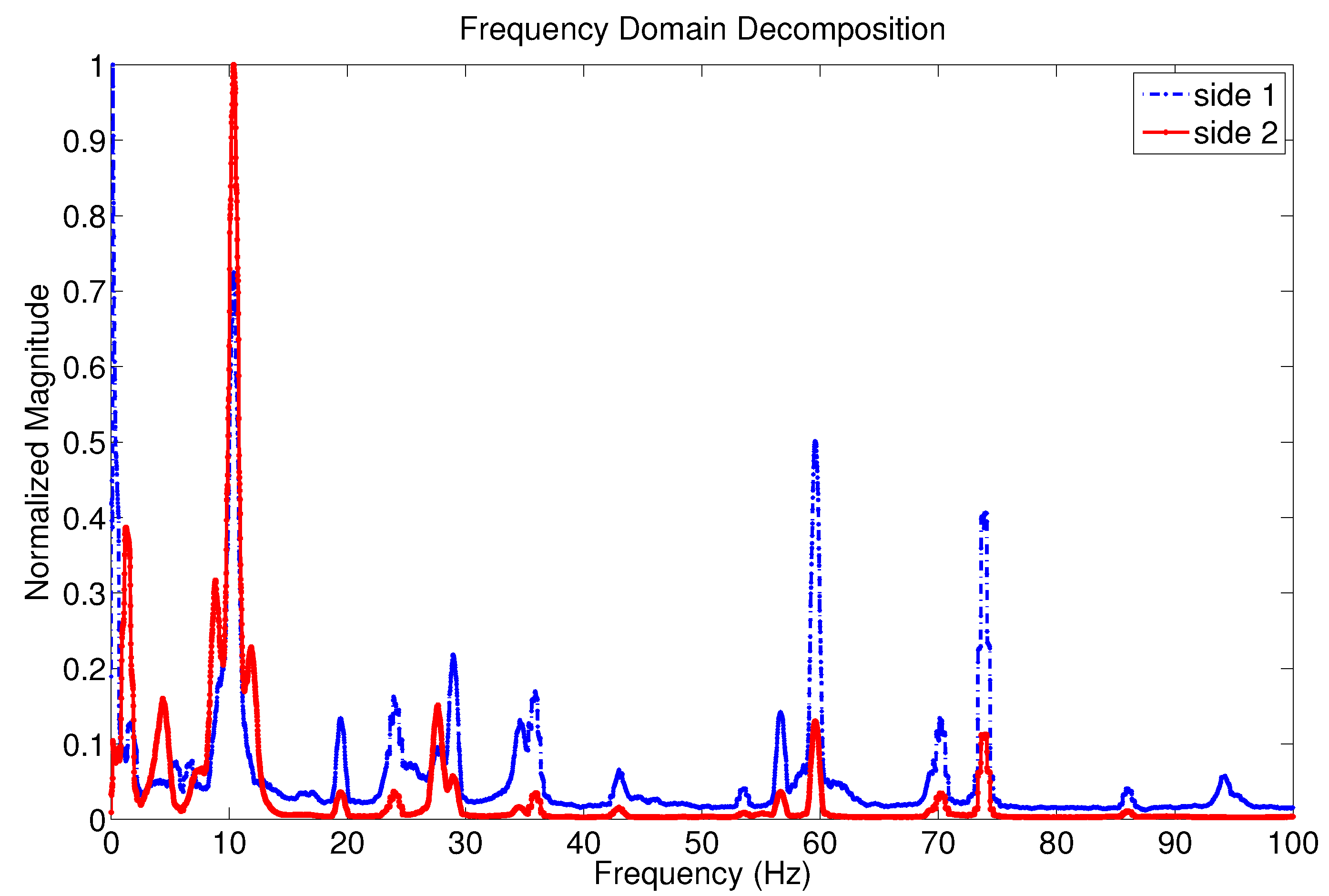
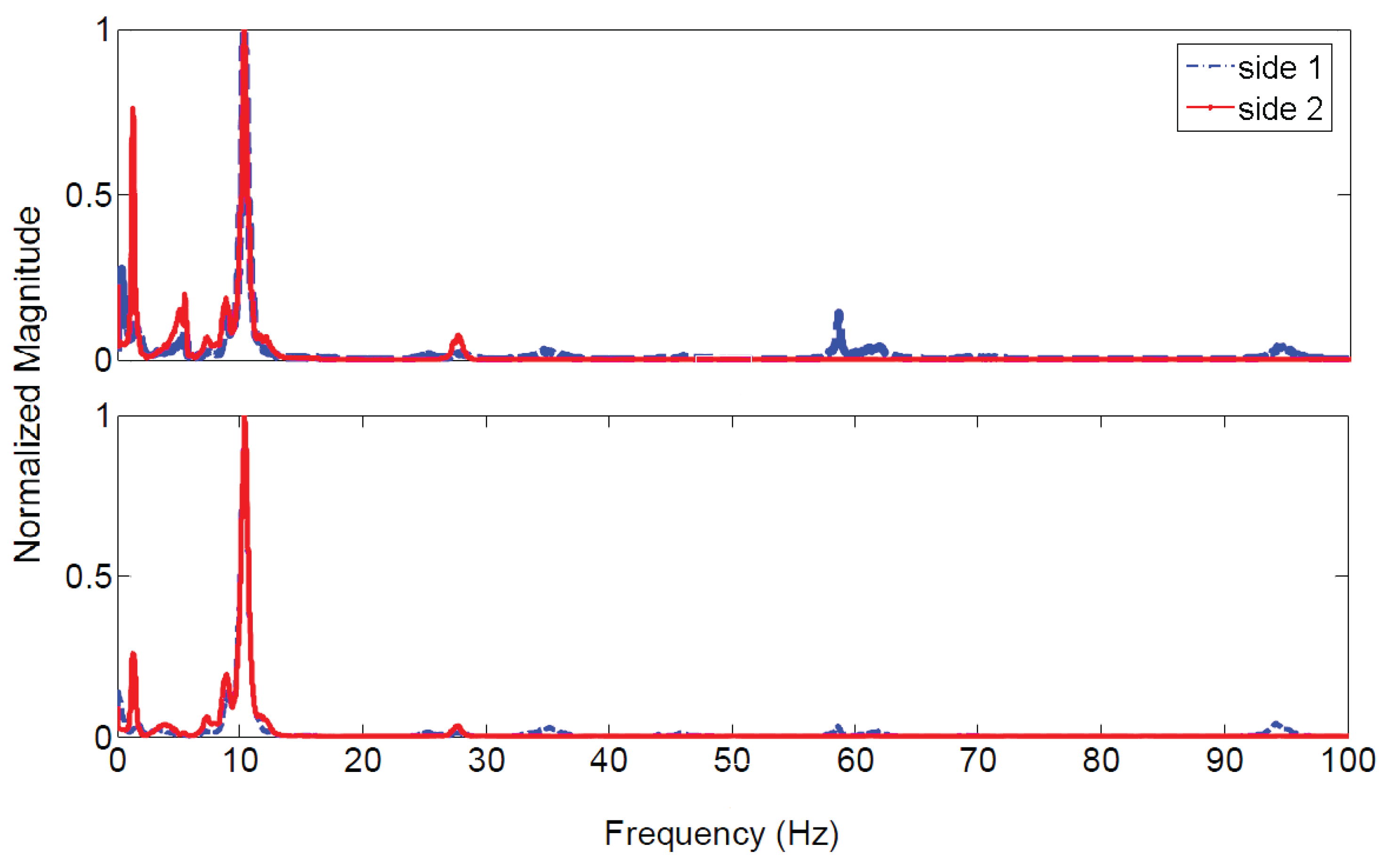
2.2. Frequency Domain Decomposition

The Frequency Domain Decomposition (FDD) technique is a non-parametric operational modal analysis technique introduced by Brincker et al. [17]. It is very similar to the Complex Mode Indicator Function (CMIF) introduced by Shih et al. [18], but applied to a matrix of spectra (multi-input and multi-output), rather than FRFs. In the FDD technique, the first step is to estimate the PSD matrix. The calculation of the output PSD [$G_{yy}\left(j\omega \right)$] at discrete frequencies ($\omega ={\omega }_i$) is then decomposed by taking the SVDof the matrix:

$$G_{yy}\left(j\omega \right)=U_i{S}_i{V}_i^H$$

(1)

where the matrix, $U_i=\left[u_{i1}{u}_{i2}...u_{im}\right]$, is a unitary matrix holding the singular vectors and $S_i$ is a diagonal matrix holding the singular values [19]. In the case of real valued matrices, the $V^H$ is a simple transpose. Near the peak corresponding to the $k^{th}$ mode in the spectrum; the singular value will dominate, and the first singular vector, $u_{i1}$, is an estimate of the mode shape:

$$\varphi =u_{i1}$$

(2)

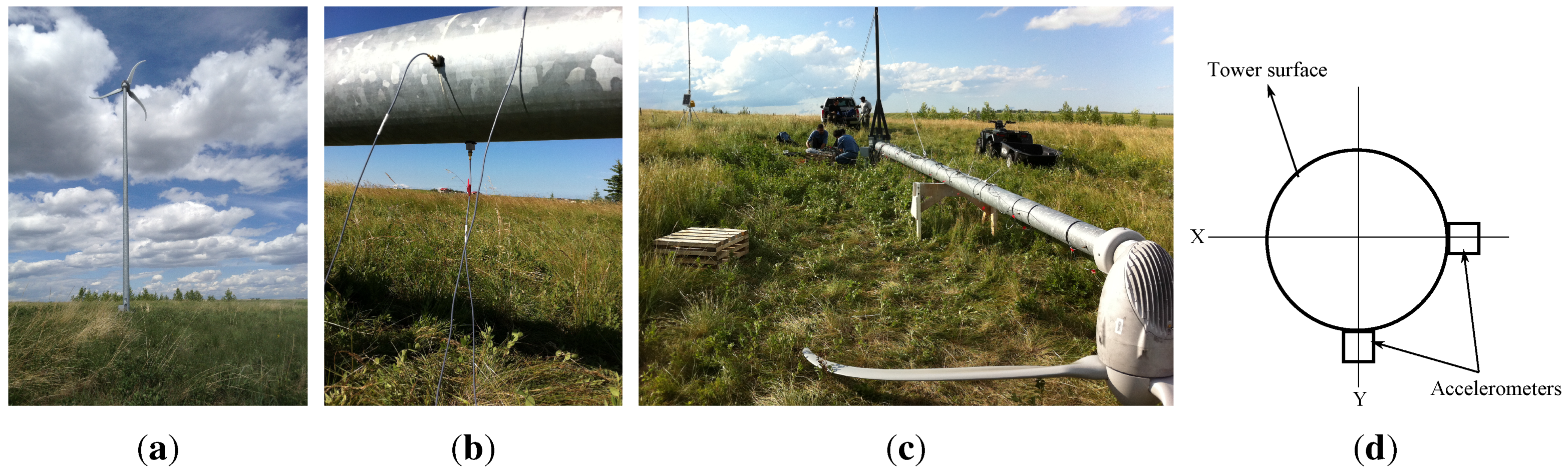
2.3. Tower Vibration

The height of the Skystream tower was 10.2 m, the base outer diameter was 27.56 cm and the top outer diameter was 15.67 cm with the thickness of 3.416 mm. The tower was made from S105 grade steel [20]. In terms of modal and vibration analysis, the tower and turbine can be considered as a beam with a mass or moment of inertia at the top representing the nacelle and blades with a known centre of mass. In other words, although blades have an aerodynamic interactions with the tower, the natural frequencies of the tower are affected only by the top mass and the centre of mass. Therefore, to avoid the complex geometry of the nacelle and turbine, their masses were simply combined (to give 77 kg) and applied at the centre of mass, 400 mm from the axis of the tower.

Table 1. Natural frequencies calculated by the FEModel; the direction can be found from Figure 3d.

Mode	Frequency (Hz)	Direction	Mode	Frequency (Hz)	Direction
1	1.378	X	7	31.73	Y
2	1.379	Y	8	42.33	X
3	9.74	X	9	61.34	Y
4	9.92	Y	10	70.18	X
5	20.57	Y	11	101.53	X
6	24.97	X	12	107.43	Y

Table 1. Natural frequencies calculated by the FEModel; the direction can be found from Figure 3d.

Mode	Frequency (Hz)	Direction	Mode	Frequency (Hz)	Direction
1	1.378	X	7	31.73	Y
2	1.379	Y	8	42.33	X
3	9.74	X	9	61.34	Y
4	9.92	Y	10	70.18	X
5	20.57	Y	11	101.53	X
6	24.97	X	12	107.43	Y

Natural frequencies are shown in Table 1 in the low-frequency range (≤100 Hz). The first two pair of modes, at 1.378, 1.379 and 9.74, 9.92 Hz, are very close to each other, implying that they can be excited at the same time, but in different directions (orthogonal directions). However, higher modes are well separated. This is important, since if the excitation load, for example, contains a component at 10 Hz, then it can generate resonances in both down/up-wind and side-wind vibration at the same time. Basically, there are six modes between 0–110 Hz in each direction, giving twelve resonances in total. X is the wind direction and Y the wind-side direction. This information will be used later for experimental comparison.

Figure 3. Accelerometers attached on the tower.

Figure 3. Accelerometers attached on the tower.

2.3.1. Experiment Results

Figure 3 shows the studied SWT. The turbine is no longer supplied with this height of tower. This is most likely to do with it being too short to be exposed to high winds and not due to any other inherent problems. The rated output power is 2.4 kW with a three-bladed downwind rotor with stall-regulation and a control system that attempts to maintain the optimum tip speed ratio over a wide range of wind speeds. Thus, the rotor speed shown in the subsequent results can be taken as a rough indicator of the wind speed, which was not measured in these experiments. The rotor diameter was 3.72 m. The turbine is allowed to yaw freely with yaw stability provided by the downwind deflection of the blades. Twenty four accelerometers were used, because that was the maximum number available, and the greater the number of accelerometers, the better the resolution of the mode shapes. They were attached along two orthogonal lines to the tower. The tower was lowered and raised using the gin pole and truck seen in Figure 3c and was bolted to the foundations as a normal installation for the duration of these experiments. The single-axis B&K 4508-B piezoelectric accelerometers were spaced equally apart, at approximately 90 cm; see Figure 3. The data acquisition module (DAQ) was a portable National Instruments NI9234 with a minimum sampling rate of 1.652 kHz. Several data collections were done over periods of 15 to 30 min to capture low frequencies and changes in operating conditions. Most of the measurements were done only for vibration analysis; however, the last one was synchronized to a wireless module connected to the antenna at the top of the turbine to record the rotor angular velocity and output power. During the whole measurement, the SWT reached a maximum output power of about 460 W, as shown in Figure 4. At the very beginning of data acquisition, the blades reached 150 rpm, and the output power reached 55 W. In the middle of data collection, there was no wind and, consequently, no power generation. However, the wind speed increased for the final section of the log, and as a result, the turbine reached about 460 W.

Figure 4. Power and blade speed logs.

Figure 4. Power and blade speed logs.

Considering 12 accelerometers on each side will yield the following matrices:

$$\begin{array}{c}\hspace{1em}{G}_1\left(j\omega \right)=\left[\begin{array}{cccc}PS{D}_{1,1}\left(j\omega \right)& CS{D}_{1,2}\left(j\omega \right)& \cdots & CS{D}_{1,12}\left(j\omega \right)\\ CS{D}_{2,1}\left(j\omega \right)& PS{D}_{2,2}\left(j\omega \right)& \cdots & CS{D}_{2,12}\left(j\omega \right)\\ ⋮& ⋮& \ddots & ⋮\\ CS{D}_{12,1}\left(j\omega \right)& CS{D}_{12,2}\left(j\omega \right)& \cdots & PS{D}_{12,12}\left(j\omega \right)\end{array}\right]\hfill \\ G_2\left(j\omega \right)=\left[\begin{array}{cccc}PS{D}_{24,24}\left(j\omega \right)& CS{D}_{24,23}\left(j\omega \right)& \cdots & CS{D}_{24,13}\left(j\omega \right)\\ CS{D}_{23,24}\left(j\omega \right)& PS{D}_{23,23}\left(j\omega \right)& \cdots & CS{D}_{23,13}\left(j\omega \right)\\ ⋮& ⋮& \ddots & ⋮\\ CS{D}_{13,24}\left(j\omega \right)& CS{D}_{13,23}\left(j\omega \right)& \cdots & PS{D}_{13,13}\left(j\omega \right)\end{array}\right]\hfill \end{array}$$

(3)

where diagonal elements, PSD, represent cross-correlation between the same channels, usually called auto-correlation, and CSD, off-diagonal elements, represent cross-correlation between different channels. “1” and “2” indicate different sides (X and Y) similar to Figure 3d. Using Equation (3) allows examination of all channels as the reference channel and various combinations with other channels. After building these matrices, SVD was applied for each frequency up to 100 Hz. Furthermore, it was applied on different sections of the collected data, for example, when wind is blowing or not with different defined overlaps. Figure 5 shows the excited frequencies for the whole collected data from one of the measurements with different wind speed and power regimes, as was shown in Figure 4. “Side 1” and “Side 2” represent “X” and “Y”, as shown in Figure 3d, respectively. It should be mentioned that these two sides have been defined based on wind direction initially; yet, it was observed that the rotor plane rotates during the the measurement campaign. Thus, the X and Y directions also yawed. Because the acceleration amplitudes were too low to distinguish the peaks, magnitudes were normalized to the maximum value. The highest values occurred in the range 0–10 Hz, implying the higher contribution of lower modes in vibration generation. The noticeable peaks are listed in Table 2 and can be compared to FEM determination of the natural frequencies in Table 1. It should be noted again that Table 2 represents frequency components of one sample among different measurements. There are many forced frequencies in the table, which are absent in other measurements. In other words, the frequency components, which are common to most measurements, can be interpreted as natural frequencies, and the ones occurring in only some of the measurements are forced components. As a result, No. 2, 5, 7, 8, 10, 13, 15, 16 and 19 represent natural frequencies. Other than wind excitation, blade and generator rotational frequencies might have excited the tower. Thus, the assumption of OMA that the input force is white Gaussian noise could be violated. To determine which frequencies were excited while only wind is the input force, the data from the middle section of the Figure 4 was taken (i.e., 300 s to 600 s). It was divided in two halves with 33% overlap to average the two parts. Frequency responses were then determined and plotted in Figure 6. Although there are small peaks at higher frequencies, it seems that wind itself did not excite all resonance modes. First mode (1.3 Hz) and second mode (10.4 Hz), on the other hand, resonated easily. The conclusion here is that wind cannot excite all resonances, even though it is commonly assumed as broadband input.

Figure 5. Excited frequencies for the entire data collection period.

Figure 5. Excited frequencies for the entire data collection period.

Table 2. Excited frequencies calculated by Frequency Domain Decomposition (FDD) below 100 Hz.

No.	Side 1	Side 2	No.	Side 1	Side 2
1	0.15	0.16	11	34.6	33.8
2	-	1.33	12	35.9	36.7
3	-	4.48	13	43.1	45.2
4	-	8.82	14	56.6	-
5	10.4	10.3	15	59.7	58.8
6	-	11.9	16	70.3	72.9
7	19.5	21.3	17	73.8	-
8	23.9	-	18	85.9	85.4
9	28.9	27.5	19	94.02	-
10	-	29.5	20	-	-

Table 2. Excited frequencies calculated by Frequency Domain Decomposition (FDD) below 100 Hz.

No.	Side 1	Side 2	No.	Side 1	Side 2
1	0.15	0.16	11	34.6	33.8
2	-	1.33	12	35.9	36.7
3	-	4.48	13	43.1	45.2
4	-	8.82	14	56.6	-
5	10.4	10.3	15	59.7	58.8
6	-	11.9	16	70.3	72.9
7	19.5	21.3	17	73.8	-
8	23.9	-	18	85.9	85.4
9	28.9	27.5	19	94.02	-
10	-	29.5	20	-	-

Figure 6. Two sets of data used for Frequency Domain Decomposition (FDD) analysis with 33% overlap (300 s to 600 s) : (Top) First 66% of data, (Bottom) Second 66% of data.

Figure 6. Two sets of data used for Frequency Domain Decomposition (FDD) analysis with 33% overlap (300 s to 600 s) : (Top) First 66% of data, (Bottom) Second 66% of data.

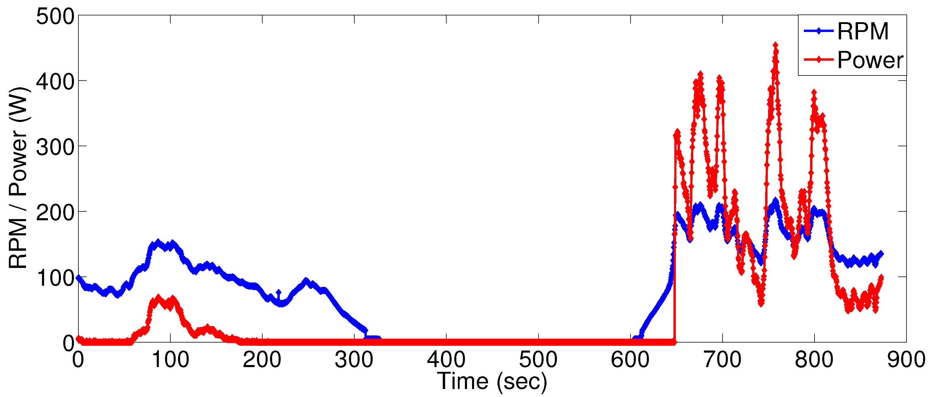
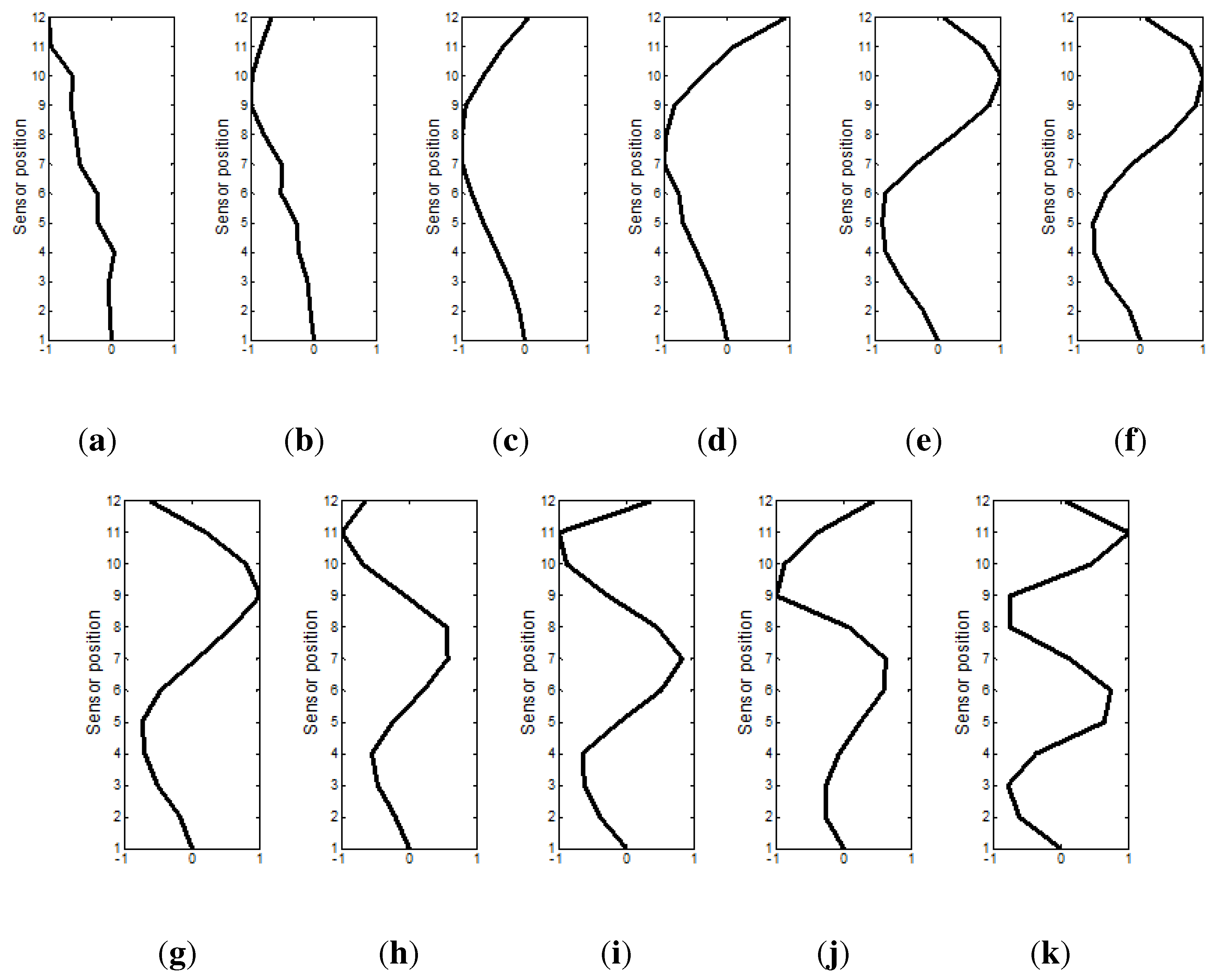
2.3.2. Operational Deflection Shapes Analysis

Operational deflection shape (ODS) is typically the deflection of a structure at a specific frequency. ODS analysis is a way to visualize the motion in response to the input forces and may be different from the mode shape, where the structure is acted on by known external forces. A motion can be described by a vector, including locations and directions. It is either a set of time domain responses at a particular time or frequency domain values at a specific frequency. These deflections are the motion of one point relative to others and are not scaled. Since ODS is a relative motion, it requires a fixed reference point. In this analysis, the bottommost channels at both directions (X and Y) were chosen, since they are connected near the tower’s base, which did not move. Figure 7 shows ODSs at the resonance frequencies, which can be interpreted as unscaled mode shapes; therefore, they were normalized to the maximum displacement value. It can be seen that they are in good agreement with familiar mode shapes of a horizontal cantilever beam, unlike other frequencies, which are forced frequencies.

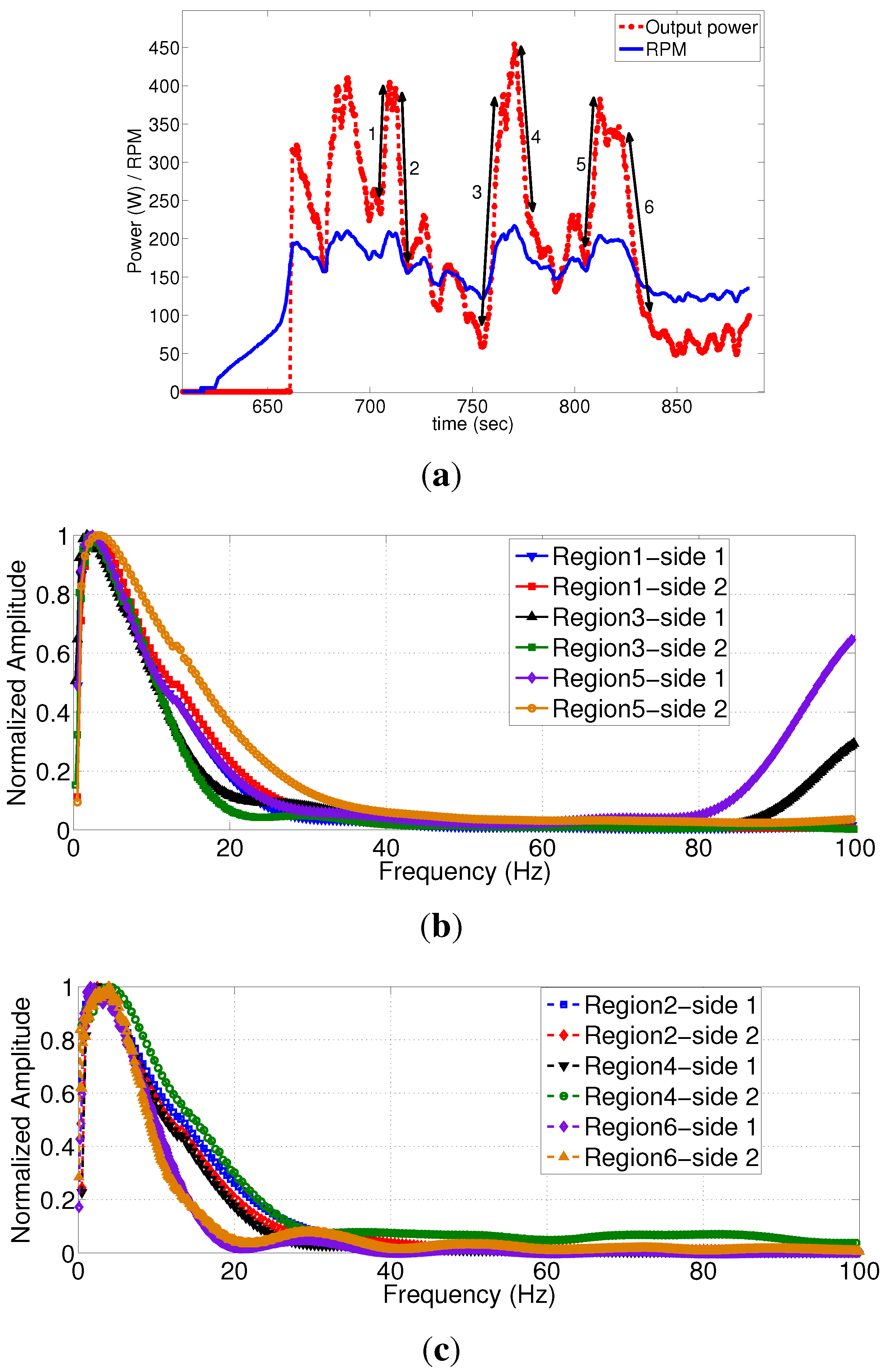
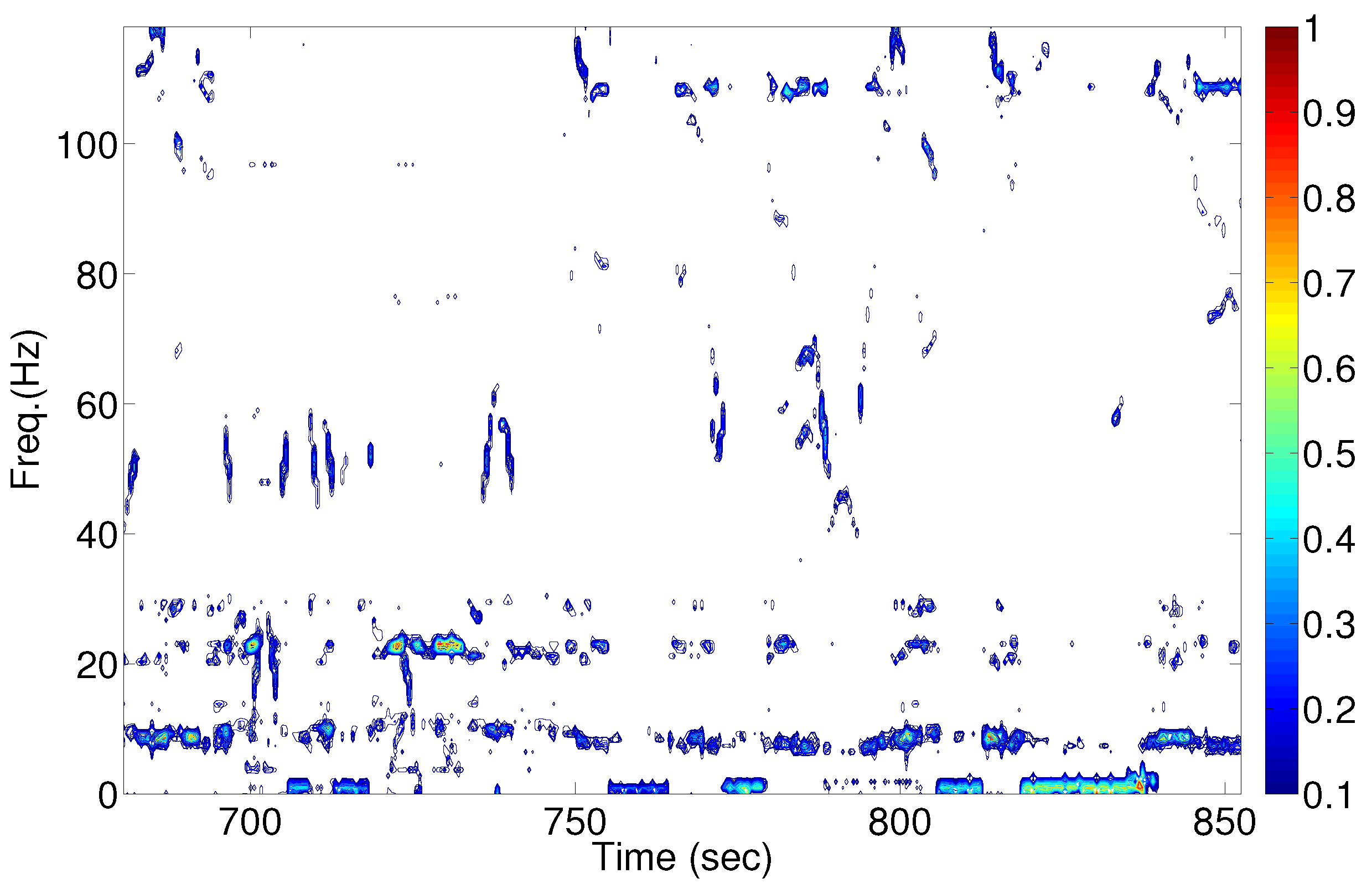
2.3.3. Short-Time Fourier Transform

In the previous section, there was an inherent assumption that the wind and any other exciting forces exhibit stationary white Gaussian noise behaviour and, therefore, are not time-varying. Yet, all sources in this study were time-varying. For example, blade rotational speed and its interaction with the tower changes with wind speed, and so do components inside of the nacelle. All these sources affect the tower simultaneously, and consequently, the fundamental assumption is violated. This explains the many frequencies evident in Figure 5. To investigate the time dependency further and observe how frequencies vary with time, output power and blade speed, Short-time Fourier Transforms (STFT) can be used. Since the data used in this study are discrete, the discrete-time STFT is applied, which breaks the data up into many pieces, which commonly have overlaps to minimize the artifacts at the boundaries. Each piece is then transformed by Fourier transform containing magnitudes for each frequency.

Figure 7. Operational deflection shapes (ODSs) on both sides. The horizontal axes show the normalized relative motions. (a) 1.33 Hz(X); (b) 1.33 Hz(Y); (c) 10.3 Hz(X); (d) 10.4 Hz(Y); (e) 21.3 Hz(Y); (f) 23.9 Hz(X); (g) 29.5 Hz(Y); (h) 43.1 Hz(X); (i) 58.8 Hz(Y); (j) 70.3 Hz(X); (k) 94.2 Hz(Y).

Figure 7. Operational deflection shapes (ODSs) on both sides. The horizontal axes show the normalized relative motions. (a) 1.33 Hz(X); (b) 1.33 Hz(Y); (c) 10.3 Hz(X); (d) 10.4 Hz(Y); (e) 21.3 Hz(Y); (f) 23.9 Hz(X); (g) 29.5 Hz(Y); (h) 43.1 Hz(X); (i) 58.8 Hz(Y); (j) 70.3 Hz(X); (k) 94.2 Hz(Y).

As shown by Figure 4, the maximum power and angular velocity occurred at the end of the the data collection from around 670 s to 850 s. For this time period, STFT was applied on each second to plot Figure 8. This resolution was chosen in order to avoid poor frequency resolution. Basically, a wide window gives better frequency resolution, but poor time resolution, and a narrower window gives good time resolution, but poor frequency resolution. Since this analysis deals with very low frequencies, the time resolution should not be too small, and on the other hand, to keep frequency resolution reliable, the time window should not be too large, either. Normalized magnitudes are specified by a contour bar varying from white to red, representing zero to one, respectively. Apparently, the frequency of 10 Hz was excited for most of the record. This frequency corresponds to the second bending mode. The fourth bending mode at 23 Hz was also excited with several high magnitude peaks. Besides, the frequency band of 40–60 Hz shows many peaks, which are almost vertical lines. This behaviour impliesforced frequency.

Figure 8. Spectrogram of the last section of collected data. The contour bar displays the normalized amplitude.

Figure 8. Spectrogram of the last section of collected data. The contour bar displays the normalized amplitude.

There are other small points and peaks, especially at the middle of the plot. This illustrates that the frequency bands above 30 Hz were not excited strongly, and therefore, they do not contribute significantly to the vibration. This conclusion supports the conclusion from Figure 5 and Figure 6.

Another noticeable dominant peak happened at very low frequency, below 2 Hz. These clusters, most noticeable around 710 s and 770 s and, then, between 805 s and 840 s, correspond to the first fundamental bending mode. An interesting fact about them is that they occurred during discrete times with considerable gaps, unlike the second and third modes.

To study these regions, output power and blade speed logs were decomposed, as indicated by Figure 9a. There are six regions: 1, 3 and 5, when the rotor was accelerating, and 2, 4 and 6, when decelerating continuously. Considering the maximum blade speed of 250 rpm, the blade rotation frequency reached 12.5 Hz. Figure 9c,d shows the frequency domain response for these regions. The only frequency excited was 1.3 Hz, corresponding to the first bending mode. The range of blade passing frequency is between 6 to 11 Hz, which is much higher than the dominant peak and closer to the second mode, which was observed from Figure 8. Therefore, the conclusion is that when the wind speed increases or decreases, causing the power level to increase or decrease, respectively, most of the vibration occurs in the first natural mode. This is consistent with the previous analysis, where it was found that most of the vibration occurs in the range of 0–20 Hz.

Figure 9. Last section of data. (a) Zoomed in power/rpm logs; (b) blades accelerating; (c) blades decelerating.

Figure 9. Last section of data. (a) Zoomed in power/rpm logs; (b) blades accelerating; (c) blades decelerating.

3. Small Wind Turbine Noise

Noise measurement of a SWT is difficult, because the turbine noise is generally submerged in the background, and there are many fewer studies than for large wind turbine noise emission.

Wood [21] published measurements and predictions of noise from a 5 kW horizontal-axis SWT at 15 m from the hub. Although there was an equipment failure, he concluded the output noise was only 2–3 dBA more than background noise.

Husky and Meadors et al. [22] published noise measurements on a 900 W SWT. The rotor was mounted on a 30 ft tower with the rotor diameter of 2.1 m. The blade speed varied up to 1,200 rpm. The overall sound at 10 m from the turbine’s base changed 13 dB, while wind speed varied from 6 to 13 m/s. The turbine-only noise increased faster than the background noise level. The turbine-only noise level varied between 55 to 67 dBA in the range of 4 and 13 m/s.

A comprehensive study was conducted by Migliore et al. [23] on six different SWTs. The rated output power range varied from 400 W to 100 kW. The authors mentioned the tedious calculations, due to wind speed variations, and also the small difference between background and turbine noise levels. In some cases, this difference was less than 6 dBA. A reasonable alternative is to compute the noise emission.

The analysis of acoustic wave propagation from and inside a wind turbine tower requires a flexible analysis tool capable of representing the thin-walled tower with propagation speed and density variations, as well as frequency-dependent attenuation mechanisms. Over the past decades, many computer-based, numerical formulations have been developed in order to extend the analytical wave equations to more sophisticated modelling configurations, either in the time or frequency domains, such as [24].

Among the variety of formulations, the Finite-Element Method (FEM) numerical technique is recognized to be the most versatile. FEM is able to calculate strains, stresses, deformations in the solid domains and, also, the pressure and velocity in fluids. However, FEM cannot deal with infinite boundaries. In other words, there are significant errors on the open boundary conditions if the the computational domain is not large enough to simulate infinite fluids. The larger domain may possibly be inefficient to implement. To avoid this restriction, one can use an Absorbing Boundary Condition (ABC) defined on the very outer boundaries, such that the scattered acoustic wave can only propagate outwards through the boundaries, and artificial reflections due to the domain limitation are minimized [25].

There are ample works describing general acoustic-structure modelling and wave propagation, such as [26]. However, the authors are only aware of one relevant publication on wind turbine structure interaction with surrounding air. Marmo et al. [27] used a commercial package in order to predict noise level. The simulation was performed for a large wind turbine, and the author did not give any more details on the size of the turbine and tower. There was a lack of appropriate force definition. The simple harmonic analysis was performed without considering any drag or thrust loads. The predicted noise level at a distance of 20 m from the tower’s base reached 60 dB between 600 to 900 Hz, while at the low-frequency band, it reached less than 10 dB. Minimizing the vibration transferred from the gearbox to the tower and the potential noise amplification using damping materials was the author’s motivation.

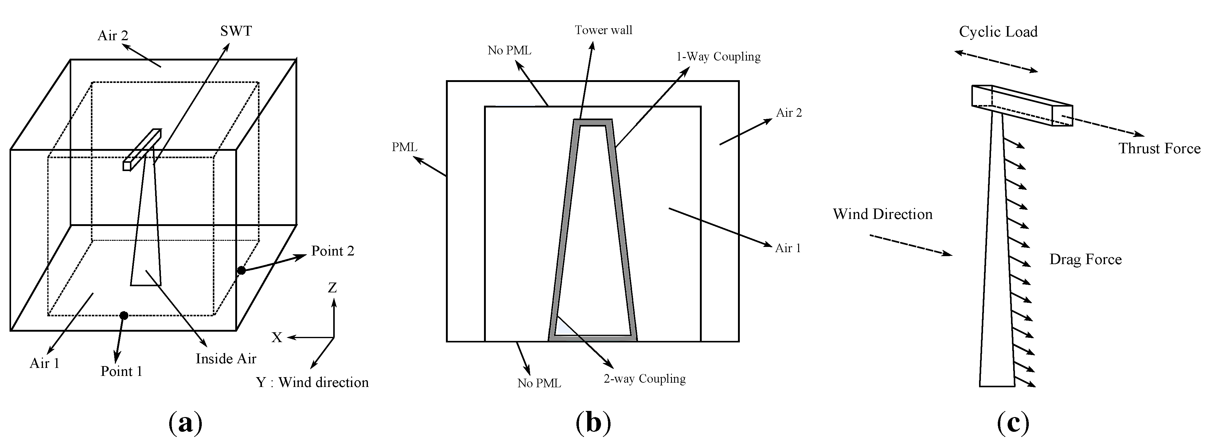
3.1. Acoustic Finite-Element Equations

Acoustic-structure interaction problems are solved by coupling the wave equation and the structural dynamics equation In other words, these two domains need to be coupled with some mandatory assumptions [28]. The fluid material must be compressible to allow acoustic waves, but the pressure gradients with respect to the static pressure are small enough to assume constant density. The fluid is inviscid with constant mean pressure. There are no gyroscopic or Coriolis nonlinearities present.

The linear acoustic wave equation is given by the Helmholtz equation:

$$\frac{1}{c^2}\frac{{\partial }^{2}P}{\partial t^2}-{\nabla }^{2}P=0$$

(4)

where c is the speed of sound in fluid determined by $c=\sqrt{\frac{k}{{\rho }_0}}$; ${\rho }_0$ and k are static fluid density and the bulk modulus of fluid, respectively; P is acoustic pressure, depending on the specific location and time [$P(x,y,z,t)$]; and t represents time [29,30]. Then, the discretized wave equation is written in a finite element matrix form by:

$$\left[{M_e}^P\right]\{\ddot{P_e}\}+\left[{K_e}^P\right]\left\{P_e\right\}=0$$

(5)

where $\left[{M_e}^P\right]$ and $\left[{K_e}^P\right]$ are the fluid mass and stiffness matrix, respectively. These formulations and notations are described in [31]. The fluid-structure coupling is created by setting the pressure gradient of the fluid equal to the acceleration of the structure at the interface:

$$\left\{n\right\}\left\{\nabla P\right\}=-{\rho }_0\left\{n\right\}\frac{{\partial }^2\left\{u\right\}}{\partial t^2}$$

(6)

where $\left\{u\right\}$ and $\left\{n\right\}$ are displacement vector of the structure at the interface and the unit normal at the fluid boundary, respectively. Taking the fluid-structure interface condition into account in the wave equation [Equation (4)] and, then, re-writing it in the FE matrix form gives the following equation:

$$\left[{M_e}^P\right]\{\ddot{P_e}\}+\left[{K_e}^P\right]\left\{P_e\right\}+{\rho }_0{\left[R_e\right]}^T\left\{\ddot{u_e}\right\}=0$$

(7)

where ${\rho }_0\left[R_e\right]$ is the fluid-structure coupling mass matrix. Dissipation of energy, because of damping at the fluid boundary, can be added by a term to Equation (7) [28]:

$$\left[{M_e}^P\right]\{\ddot{P_e}\}+\left[{C_e}^P\right]\left\{\dot{P_e}\right\}+\left[{K_e}^P\right]\left\{P_e\right\}+{\rho }_0{\left[R_e\right]}^T\left\{\ddot{u_e}\right\}=0$$

(8)

where $\left[{C_e}^P\right]$ is the fluid damping matrix. Similar to the load acting on the fluid interface from the structure, a load from fluid forcing on the structure interface may be defined as ${F_e}^{pr}$ and included in the structural dynamics equation:

$$\left[M_e\right]\left\{\ddot{u_e}\right\}+\left[C_e\right]\left\{\dot{u_e}\right\}+\left[K_e\right]\left\{u_e\right\}=\left\{F_e\right\}+\left\{{F_e}^{pr}\right\}$$

(9)

where $\left\{{F_e}^{pr}\right\}=\left[R_e\right]\left\{P_e\right\}$ is the fluid pressure load vector on the interface. Equations (8) and (9) are FE equations, and then they are combined as [28]:

$$\left[\begin{array}{cc}\left[M_e\right]& \left[0\right]\\ \left[M^{fs}\right]& \left[{M_e}^P\right]\end{array}\right]\left[\begin{array}{c}\left\{\ddot{u_e}\right\}\\ \{\ddot{P_e}\}\end{array}\right]+\left[\begin{array}{cc}\left[C_e\right]& \left[0\right]\\ \left[0\right]& \left[{C_e}^P\right]\end{array}\right]\left[\begin{array}{c}\left\{\dot{u_e}\right\}\\ \{\dot{P_e}\}\end{array}\right]+\left[\begin{array}{cc}\left[K_e\right]& \left[K^{fs}\right]\\ \left[0\right]& \left[{K_e}^P\right]\end{array}\right]\left[\begin{array}{c}\left\{u_e\right\}\\ \left\{P_e\right\}\end{array}\right]=\left[\begin{array}{c}\left\{F_e\right\}\\ \left\{0\right\}\end{array}\right]$$

(10)

where $\left[M^{fs}\right]={\rho }_0{\left[R_e\right]}^T$ and $\left[K^{fs}\right]=-\left[R_e\right]$.

3.1.1. Coupling

Whenever an elastic component is fully or partially in contact with the surrounding fluid domain, both structural vibration and fluid pressure are influenced by vibro-acoustic interaction. The strength of the vibro-acoustic coupling mainly depends on the structure and the fluid domain’s size, as well as the material properties and the strength of the input forces. Based on the strength of the interaction, vibro-acoustic systems are classified into uncoupled (one-way coupling) and coupled (two-way coupling) systems. For most noise emission problems, the coupling is one-way, that is, the fluid adjacent to the structure is excited by the structure, but the structural dynamics is not influenced by the fluid. This is the case for the external air. The air within the tower, however, may influence the structure, and thus, the coupling is two-way. More details will be discussed in Section 3.2.

3.2. Finite-Element Acoustic Analysis of Tower Noise Emission

This section reproduces the main results in [32], but with more detail and explanation. Three acoustic bodies were added in order to couple the structural vibration of the tower to the fluid/acoustic domain. The first and main one represents the computational domain, which is called “Air 1” in this section, while “Air 2”, the outer domain, is used to avoid any reflections on the boundaries. Last, but not the least, “Inside Air” is the separate air domain inside of the tower. This configuration schematically is shown in Figure 10a.

“Air 1” is a cube with the dimension chosen in reference to IEC 61400-11 [1]. “Air 2” is an enclosure with 1 m greater than “Air 1”. The foundation of the tower was immobile. All other faces were allowed free three-dimensional motions. This domain was defined to be “one-way coupled”, because it was assumed that the wave propagation in such a large domain in reality would not influence the vibration of the tower. “Air 2” had the same fluid properties as “Air 1”. However, as shown in Figure 10b, absorbing boundary conditions were added on all the outer faces, except the ground. “Inside Air” shared the same material properties as “Air 1” and “Air 2”, but was coupled to the tower, because the space inside of the tower is too small to neglect the pressure on the structure.

Figure 10. FE model. (a) Model schematic; (b) boundary properties; (c) loads on structure.

Figure 10. FE model. (a) Model schematic; (b) boundary properties; (c) loads on structure.

3.3. Simulation

The simulations require the external loads. The loads on the tower used here are rough approximations, as determined from the simple load model of IEC 61400-2, the international safety standard for small wind turbines [33].

3.3.1. Thrust Force

One of the main loads is the turbine thrust (T), which is given by:

$$T=\frac{1}{2}{C}_T\rho U^{2}A$$

(11)

where $C_T$, ρ, U and A are thrust coefficient, air density, wind speed and blade swept area, respectively [34]. This load increases by the square of the wind speed, so high speeds induce high loads, which could be problematic. This load was assumed to act through the rotor axis, which is a reasonable approximation for SWTs, which do not experience large variations in wind speed across the rotor. This axis is shown by Figure 10c. Wind speed was set as 6 m/s, a common operational speed. At the Betz limit (where most turbines try to operate) [34], the thrust coefficient, $C_T$, is theoretically 8/9. Therefore, 1.0 is a common assumption [35]. Thus:

$$T=239N$$

(12)

3.3.2. Tower Drag

Drag on the tower, as shown in Figure 10c, can be significant. For a tower of a circular section, the drag, D, is given by:

$$D=\frac{1}{2}{C}_D\rho U^{2}d$$

(13)

where $C_D$ and d are drag coefficient and cylinder diameter, respectively [34]. Since the tower diameter changes slightly, the mean value was assumed as 21.6 cm. Therefore, at $U=6m/s$, $Re=82,710$. According to [1], $C_D\approx 1$. Even though the wind speed will vary with height, it is common to assume no variation along the tower [34]. Thus, the drag, which is uniformly distributed along the tower, has the magnitude of $5N/m$.

3.3.3. Cyclic Load

The only fluctuating load case in the IEC Simple Load Model [33], $\Delta F_{shaft}$, on the shaft, is given by:

$$\Delta F_{shaft}=\frac{3}{2}\frac{\lambda Q}{R}$$

(14)

where R is rotor radius. λ and Q are the tip speed ratio and shaft torque, respectively. Shaft torque, Q, is given by:

$$Q=\frac{P_r}{\omega }(N.m)$$

(15)

where $P_r$ is the turbine output (W). At 6 m/s wind speed, the blade rotational speed is 206 rpm, and turbine power is about 300 W. Therefore, $\lambda =6.687$, and $Q=13.90$ N.m.

Substituting these values in Equation (14) gives:

$$\Delta F_{shaft}=75N$$

(16)

3.3.4. Harmonic Analysis

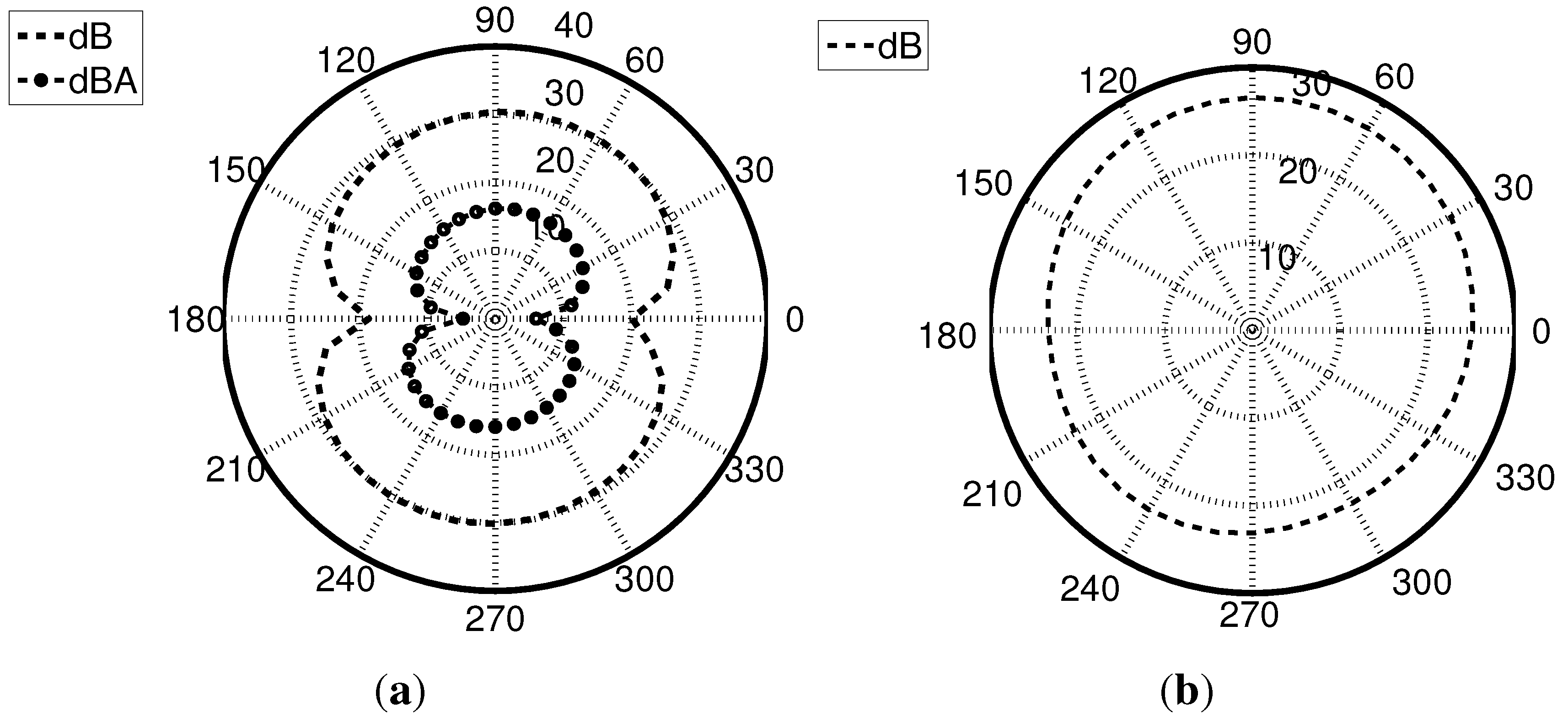
Ground level noise has been calculated in the range 0–100 Hz at 1 Hz intervals. Two locations were chosen to plot the frequency spectrum of the emitted noise, as shown in Figure 10a. Both locations were the same distance from the tower, but in different directions. They act as virtual microphones. Location 1 is downwind and Location 2 in the cross-wind direction. It should be noted that the actual SWT yaws during the operation, meaning they yaw, as well. Therefore, the noise received by any observer will often be averaged over a wide range of wind directions. Figure 11a,b shows the sound pressure level (SPL) spectrum. The most noticeable peak occurs at around 48 Hz in both locations. This frequency extends to 53 dB. Although the FEM described in Section 2.3 did not indicate any structural resonance in this region, apparently the propagated acoustic wave is sensitive to this frequency, and the main portion of the emitted noise is generated at 48 Hz. After this frequency, SPL has almost the same value at both locations between 0 to 18 dB, which can be interpreted as extremely quiet. In the Infrasound region (0–20 Hz), SPL becomes negative, even though the first and third natural frequencies have appeared as small peaks. Values less than 0 dB can be neglected. In the top figure, the third mode is shown by a peak at around 24 Hz. This can be seen around 20 Hz at the bottom the figure, as was expected. Figure 11c shows human threshold criteria taken from [36]. These values indicate that only the frequency of 48 Hz can reach the hearing threshold, and the rest are below the threshold.

Figure 11. Sound pressure level (SPL) spectrum. (a) Point 1; (b) Point 2; (c) Hearing threshold.

Figure 11. Sound pressure level (SPL) spectrum. (a) Point 1; (b) Point 2; (c) Hearing threshold.

In order to combine the generated sound at all frequencies, the overall sound pressure level was calculated. Figure 12a displays ground level dB and dBA at the same distance of 12.06 m around the tower. 90${}^{\circ }$ indicates the wind direction. It can be seen that the overall SPL varies between 26 to 32 dB for most angles, even though loads have been applied in one direction, meaning the wind direction close to the tower does not influence the emitted noise direction significantly. However, deficits appear near side directions (0${}^{\circ }$ and 180${}^{\circ }$). Removing the loads, and, therefore, a simple modal vibration, gives Figure 12b, where those deficits disappeared. Loads produced a 6 dB noise level difference. Comparison of Figure 12a,b shows the strong sensitivity of the noise to the input loads. As a rough comparison with actual turbine noise output, it was shown in [23] that the background noise is around 45 dBA at a wind speed of 6 m/s. Although the background noise is environment-specific, it can be estimated that the emitted noise from the tower would be masked out by the ambient noise, as the maximum values reached 18 dBA.

Figure 12. Overall sound pressure levels on the ground at 12.06 m. The numbers on the outside of the circles denote direction, with 90${}^{\circ }$ being the wind direction. (a) With loads; (b) without loads.

Figure 12. Overall sound pressure levels on the ground at 12.06 m. The numbers on the outside of the circles denote direction, with 90${}^{\circ }$ being the wind direction. (a) With loads; (b) without loads.

Figure 13a shows the noise level at different distances from the tower (15 to 500 m) at the height of 1 m from the ground. This height was chosen, since many of the experiments, such as [37], set the microphone at this height to avoid noise reflection from the ground. Ninety degrees represents the downwind direction. The noise levels in the downwind and upwind directions start from around 30 dB at 15 m and decrease to 12 dB at 500 m. The deficits at 0${}^{\circ }$ and 180${}^{\circ }$ and their vicinities remain for all distances. This illustrates that noise levels at side directions do not exceed 19 dB.

3.3.5. Source Type

Spreading depends on the type and location of the source. In the case of a wind turbine, the nacelle and blades are likely to be acoustically more compact than the tower, which would act as a line source at small distances. At distances much larger than the tower height, it can be assumed as a point source. This is important, because noise level attenuation is faster in hemispherical spreading than cylindrical. In general, the reduction in noise level by cylindrical pattern is 3 dB, as the distance is doubled. Therefore, noise levels at large distances are plotted to determine the source behaviour; see Figure 13b. The downwind direction was chosen for this figure, since noise in this direction is larger than for other angles, due to the wind. Doubling the distance close to the tower, say, from 30 to 60 m, reduces the noise level from 27.8 to 25.4 dB, which gives 2.4 dB of difference. This means the propagation pattern is approximately cylindrical. The corresponding difference is 4 dB when the distance is doubled from 70 to 140 m, implying a transient region between the cylindrical and hemispherical pattern. From around 200 m is the hemispherical domain, where doubling the receiver’s position decreases the noise by 6 dB. This distance is 20-times the tower height. After this point, the SPL reduction remains around 6 dB, even though the values are too low to be perceived.

Figure 13. Far-field overall sound pressure level (dB). (a) 1 m height from the ground; (b) downwind direction.

Figure 13. Far-field overall sound pressure level (dB). (a) 1 m height from the ground; (b) downwind direction.

4. Conclusions

This research investigated an aspect of small wind turbines, which was barely studied before: tower vibration characterization and noise generation. Among different sources of noise from a small wind turbine, tower noise production has always been supposed to be negligible. However, small turbines are often placed close to houses and, consequently, could annoy the residents more often than mid- or large- scale ones, which must be placed much further away. Furthermore, at small distances, the tower will behave as a line source of noise and whose noise reduces with distance more slowly than the compact noise sources of the blades and nacelle. Thus, the tower should be designed, such that noise emission will be minimized.

In the first part of the paper, Operational Modal Analysis was performed on measurements from 24 accelerometers placed on the tower in two orthogonal lines. FDD was used to extract natural frequencies and operational deflection shapes. It was observed that when the turbine was producing power, the first three natural modes resonated significantly with high magnitudes. In contrast, if the blades were not rotating and wind was the only input force, then only the first two natural frequencies were excited. This means wind itself cannot excite high structural natural frequencies. Operational deflection shapes were also calculated to validate the finite element model for further acoustic analysis. Time-frequency Analysis using short time Fourier transforms was performed, because of the time-varying nature of inputs. The first three modes were resonating as was expected. Furthermore, it was seen that when power and blade speed increased or decreased, only the first mode was excited. By considering this part of the analysis, it was concluded that most of the vibration was produced in a very low frequency band, especially below 10 Hz.

The second part of the paper described a fluid/acoustic-structure interaction simulation. Noise level measurements from the turbine structure are not often undertaken, because the total noise emission from modern small turbines is usually close to background noise. As a result, it was decided to model the structure and couple it to the wave equation to investigate the role of the tower in noise emission. Different loads due to the turbine, including thrust and cyclic loads, as well as the wind load on the tower were estimated at the wind speed of 6 m/s using the simple load model of the IEC standard for small wind turbines. In terms of frequency spectrum, it was shown that there is significant spectral content up to 53 dB at the frequency of 48 Hz, while the lower frequency band, below 35 Hz, had negative values, even though the second and third resonance modes could be just recognized from the spectrum. That is, even though 48 Hz is not a natural frequency, it could generate high noise levels, and the main contribution to the overall sound pressure level comes from this frequency. Moreover, the noise propagation is almost uniform around the tower, except at side directions with deficits. These deficits disappeared when the assumed loads were removed. The overall noise levels from the tower are small, but are very sensitive to the assumed loads. This suggests that more accurate determination of the tower-top loads would be valuable. For example, placing an accelerometer on the nacelle would yield important information on the forcing functions. The overall pressure level decreased to 10 dB at 500 m. Besides, emission pattern changed to hemispherical from cylindrical at around 200 m, which is 20-times the tower height. At this distance, the noise level was around 18 dB, which can be considered fairly quiet. Given that, the sound pressure level due to the tower vibration is negligible at distances of more than about 70 m (7-times the tower height), whereas close to the turbine, the computed overall noise level did not exceed 30 dB.

References

1. National Revewable Energy Laboratory (NREL). Wind Turbine Generator Systems-Part 11: Acoustic Noise Measurement Techniques; IEC 61400-11; International Electrotechnical Commission: Geneva, Switzerland, 2002.
2. Boccard, N. Capacity factor of wind power realized values vs. estimates. Energy Policy 2009, 37, 2679–2688. [Google Scholar] [CrossRef]
3. Lowson, M. Applications of aeroacoustic analysis to wind Turbine noise control. Wind Energy 1992, 16, 126–140. [Google Scholar]
4. Pedersen, E.; Waye, K. Perception and annoyance due to wind turbine noise—A dose–response relationship. J. Acoust. Soc. Am. 2004, 116, 3460–3470. [Google Scholar] [CrossRef] [PubMed]
5. Rogers, A.; Manwell, J.; Wright, S. Wind Turbine Acoustic Noise; Technical Report for Renewable Energy Research Laboratory: Amherst, MA, USA, 2006. [Google Scholar]
6. James, G.; Carne, T.; Lauffer, J.; Nard, A. Modal Testing Using Natural Excitation. In Proceedings of the International Modal Analysis Conference, San Diego, CA, USA, 3–6 February 1992; pp. 1208–1208.
7. Bao, Z.W.; Ko, J.M. Determination of modal parameters of tall buildings with ambient vibration measurements. Int. J. Anal. Exp. Modal Anal. 1991, 6, 57–68. [Google Scholar]
8. Prevosto, D.; Benveniste, A.; Bonnecase, D. Application of a Multidimensional ARMA Model to Modal Analysis under Natural Excitation. In Proceedings of the 8th International Modal Analysis Conference, Kissimmee, FL, USA, 29 January–1 February 1990; Volume 1, pp. 382–388.
9. Peeters, B.; de Roeck, G. Stochastic system identification for operational modal analysis: A review. J. Dyn. Syst. Meas. Control 2001, 123, 659–667. [Google Scholar] [CrossRef]
10. James, G.H., III; Carne, T.G.; Lauffer, J.P. The Natural Excitation Technique (NExT) for Modal Parameter Extraction from Operating Wind Turbines; Technical Report for Sandia National Labs: Albuquerque, NM, USA, 1993. [Google Scholar]
11. Zhang, L.; Wang, T.; Tamura, Y. A frequency–spatial domain decomposition (FSDD) method for operational modal analysis. Mech. Syst. Signal Process. 2010, 24, 1227–1239. [Google Scholar] [CrossRef]
12. James, G.; Carne, T.; Mayes, R. Modal Parameter Extraction from Large Operating Structures Using Ambient Excitation. In Proceedings of the International Society for Optical Engineering, Denver, CO, USA, 5–6 August 1996; pp. 77–83.
13. Chauhan, S.; Hansen, M.; Tcherniak, D. Application of Operational Modal Analysis and Blind Source Separation/Independent Component Analysis Techniques to Wind Turbines. In Proceedings of 27th International Modal Analysis Conference (IMAC XXVII), Orlando, FL, USA, 9–12 February 2009.
14. Tcherniak, D.; Chauhan, S.; Rossetti, M.; Font, I.; Basurko, J.; Salgado, O. Output-Only Modal Analysis on Operating Wind Turbines: Application to Simulated Data. In Proceedings of the European Wind Energy Conference, Warsaw, Poland, 20–23 April 2010.
15. Chauhan, S.; Tcherniak, D.; Hansen, M. Dynamic Characterization of Operational Wind Turbines Using Operational Modal Analysis. In Proceedings of China Wind Power, Beijing, China, 13–15 October 2010.
16. Styles, P.; Westwood, R.; Toon, S. Monitoring and Modelling the Vibrational Effects of Small Wind Turbines on the Eskdalemuir IMS Station. In Proceedings of the 4th International Meeting on Wind Turbine Noise, Rome, Italy, 11–14 April 2011.
17. Brincker, R.; Zhang, L.; Andersen, P. Modal Identification from Ambient Responses Using Frequency Domain Decomposition. In Proceedings of the 18th International Modal Analysis Conference, San Antonio, TX, USA, 7–10 February 2000; pp. 625–630.
18. Shih, C.; Tsuei, Y.; Allemang, R.; Brown, D. Complex mode indication function and its applications to spatial domain parameter estimation. Mech. Syst. Signal Process. 1988, 2, 367–377. [Google Scholar] [CrossRef]
19. Brincker, R.; Zhang, L.; Andersen, P. Output-Only Modal Analysis by Frequency Domain Decomposition. In Proceedings of the 25th International Conference on Noise and Vibration Engineering, Leuven, Belgium, 13–15 September 2000; Volume 2, pp. 717–723.
20. Southwest Windpower. Available online: http://www.windenergy.com/products/skystream/skystream-3.7 (accessed on 7 April 2013).
21. Wood, D. Noise Measurement and Prediction for Small Wind Turbines. In Proceedings of the 35th Annual Australian and New Zealand Solar Energy Society Conference, Canberra, Australia, 1–3 December 1997.
22. Huskey, A.; Meadors, M. Wind Turbine Generator System Acoustic Noise Report for the Whisper H40 Wind Turbine; NREL/EL-50034383National Renewable Energy LaboratoryGolden, CO, USA, 2001. [Google Scholar]
23. Migliore, P.; van Dam, J.; Huskey, A. Acoustic Tests of Small Wind Turbines. In Proceedings of the 42nd AIAA Aerospace Sciences Meeting and Exhibit, Reno, NV, USA, 5–8 January 2004.
24. Schenck, H.; Benthien, G. Numerical Solution of Acoustic-Structure Interaction Problems; Technical Report; Naval Ocean Systems Center: San Diego, CO, USA, 1989. [Google Scholar]
25. Clayton, R.; Engquist, B. Absorbing boundary conditions for acoustic and elastic wave equations. Seismol. Soc. Am. 1977, 67, 1529–1540. [Google Scholar]
26. Fang, B.; Kelkar, A.; Joshi, S.; Pota, H. Modelling, system identification, and control of acoustic–structure dynamics in 3-D enclosures. Control Eng. Pract. 2004, 12, 989–1004. [Google Scholar] [CrossRef]
27. Marmo, B.; Carruthers, B. Modelling and Analysis of Acoustic Emissions and Structural Vibration in a Wind Turbine. In Proceedings of the COMSOL Conference, Paris, France, 14–19 November 2010.
28. Yuhui, L. Wave Propagation Study Using Finite Element Analysis. Ph.D. Thesis, University of Illinois at Urbana-Champaign, Urbana, IL, USA, 2005. [Google Scholar]
29. Desmet, W. A Wave Based Prediction Technique for Coupled Vibro-Acoustic Analysis. Ph.D. Thesis, University of Leuven, Leuven, Belgium, 1998. [Google Scholar]
30. Khan, M.; Cai, C.; Hung, K. Acoustics Field and Active Structural Acoustic Control Modeling in ANSYS. In Proceedings of the International ANSYS Conference, Pittsburgh, PA, USA, 22–24 April 2002.
31. Howe, M. Acoustics of Fluid-Structure Interactions; Cambridge University Press: Cambridge, UK, 1998. [Google Scholar]
32. Mollasalehi, E.; Sun, Q.; Wood, D. Low-Frequency Noise Propagation from a Small Wind Turbine Tower. In Proceedings of 2nd Symposium on Fluid-Structure-Sound Interactions and Control, Hong Kong and Macau, China, 20–23 May 2013.
33. National Revewable Energy Laboratory (NREL). Wind Turbine-Part 2: Design Requirements for Small Wind Turbines, 2nd ed.International Electrotechnical Commission: Geneva, Switzerland, 2006.
34. Wood, D. Small Wind Turbines: Analysis, Design, and Application; Springer: Berlin, Germany, 2011. [Google Scholar]
35. Huleihil, M.; Mazor, G. Wind Turbine Power: The Betz Limit and Beyond. In Advances in Wind Power; InTech: Rijeka, Croatia, 2012. [Google Scholar]
36. Moorhouse, A.; Waddington, D.; Adams, M. Proposed Criteria for the Assessment of Low Frequency Noise Disturbance; Technical Report NANR45; University of Salford: Salford, UK, 2005. [Google Scholar]
37. Jakobsen, J. Infrasound emission from wind turbines. J. Low Freq. Noise Vib. Act. Control 2005, 24, 145–155. [Google Scholar] [CrossRef]