1. Introduction
Energy conservation is currently a highly important and much-discussed field of research. The increase in global energy demand has resulted in almost daily increases in energy prices; therefore, energy conservation is important for both consumers and service providers [
1]. Energy conservation can save money for consumers by reducing tariffs; on the other hand, supplying more consumers with lower energy production reduces installation costs for service providers [
2].
In this context, the smart grid is one of the most interesting fields of research for next-generation power systems. This type of grid uses a bidirectional flow of electricity and information to create a widely distributed power delivery network. The smart grid offers several advantages, such as renewable energy usage, reduced greenhouse gas emissions, increased energy efficiency due to better balance of supply and demand, improved security and reliability, and fast and effective responses to energy generation, consumption fluctuations, and catastrophic events [
3]. The catastrophic events are sudden incidents, which occur due to the occasional failure of the power system component. The achievement of energy conservation in a smart grid, either at the consumer level or at the utility level, requires analysis of the energy provided by the utility, the effectiveness of energy use by the consumer, and the losses. This type of analysis requires energy consumption to be measured at various levels in the smart grid.
Smart meters represent one of the major components of smart grids. Smart meters can be used to measure energy consumption at various points in the smart grid [
4]. The smart grid concept has been put into full use by utility companies throughout the World through the installation of smart meters in homes and commercial buildings; by 2015, approximately 60 million smart meters will be installed in the US [
5]. The smart meter is an advanced energy meter that measures a consumer’s energy consumption and provides additional information for the utility company not typically available with a regular energy meter. The smart meter can read real-time energy consumption data and securely send those data to the company [
6]. The ultimate objective of these meters is to set real-time pricing and establish demand-side management [
7].
The functional requirement of electricity for smart meters, in terms of power measurement, is the measurement of active, reactive, and apparent power. Broadly speaking, reactive power is the difference between the power used for real working (active power) and the total consumed power (apparent power). However, some electrical equipment used in industrial and commercial building—especially transformers and motors—requires an amount of reactive power in addition to active power. The reactive power in such equipment is used to generate a magnetic field, which is essential for the inductive elements in these pieces of equipment to operate [
8]. Although reactive power is required to operate several pieces of equipment, if supplied in excess, it can also make harmful effects on appliances and installed electrical infrastructure [
1].
Power factor is another term associated with power measurement in power systems. Power factor is the relationship between the active and reactive power. It indicates how effectively the electrical power is used. In other words, power factor is the ratio of active power to the apparent power. Typically, homes have power factors in the range of 70%–85%, depending on the appliances being used. However, a power factor correction mechanism can be employed to increase the power factor above 90%. Power factor correction has several benefits. It can: save money by reducing tariff; prevent electric losses; reduce peak energy demand and reduce risk of harm being done to the installed electrical infrastructure [
9].
The tremendous increase in the amount and complexity of electrical equipment has provided welcome additions to modern homes, such as electronic ballast lighting, computer monitors, and air conditioners, but these impose an additional energy burden. This has resulted in an electric distribution profile that is completely different from what was observed 50 years ago [
10]. This change in the end-user load profile is a disadvantage for the service provider, which generates tariffs based only on active power. The addition of these nonlinear loads to the power lines means that active energy no longer represents the total energy delivered. Therefore, from the above discussion it can be concluded that the reactive power measurement is necessary to bill consumers, design the compensator, power factor correction and monitor power usage.
The aim of this study is to devise a method for practical measurement of reactive power. A reactive power measurement is essential to determine the reactive power demand and to assist in improving the voltage profile introducing power factor correction mechanism. It also enables the service provider to take the proper steps to reduce revenue losses, peak energy demand and increase power generation capacity to serve more consumers [
11]. Reactive power overloads the power lines and produces excessive thermal stress on the conductors, and it is also undesirable from the service provider’s perspective. A decrease in the reactive power leads to lower expenses; once the reactive power has been measured, it can be compensated with the help of a suitable capacitor or a number of capacitors [
2].
In this paper, we propose a more suitable implementation of the discrete wavelet transform (DWT) that uses a recursive pyramid algorithm (RPA) for reactive energy measurement in smart meters. This paper also investigates the effect of varying different system parameters such as the sampling rate, dc offset, phase offset, linearity error in current and voltage sensors, analog to digital converter resolution, and number of harmonics in a non-sinusoidal system on the reactive energy measurement using DWT. The error analysis is depicted in the form of the absolute difference between the measured and the true value of the reactive energy.
The rest of the paper is organized as follows:
Section 2 discusses some of the related work.
Section 3 discusses the different methods for measuring reactive power, their categorization, and the challenges involved with each of them.
Section 4 describes reactive power measurement using the DWT and
Section 5 suggests DWT implementation.
Section 6 presents the results for different case studies and shows the impact of various kinds of errors.
Section 7 provides some concluding remarks.
2. Related Work
Definitions and approaches for measuring reactive power have been developed in the time domain [
12,
13], Fourier (frequency domain) [
14,
15,
16], and the wavelet domain (time-frequency domain) [
17,
18,
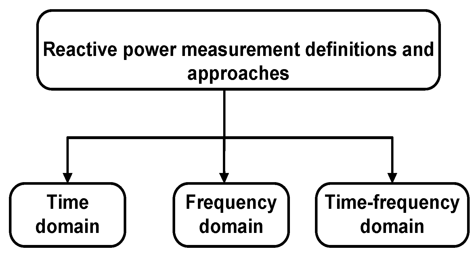
19]. The limitation of time domain definitions is that they cannot measure the reactive power for a specific frequency component and they also result in loss of temporal insights. Therefore, time-frequency (wavelet domain) analysis emerges as the most appropriate solution for measurements in power systems, because it preserves both temporal and spectral relationships associated with the resulting power [
17]. A comprehensive survey of the categories shown in
Figure 1 has been presented in [
20]. The present paper focuses on wavelet-based power measurement in the smart meter.
Figure 1.
Categories of reactive power measurement definitions and approaches.
Figure 1.
Categories of reactive power measurement definitions and approaches.
The advantage offered by wavelet domain analysis has been exploited by many studies on power measurement reported in the literature. For example, Yoon and Devaney [
21] introduced the concept of power measurement using the DWT. In [
2], the same authors proposed a calculation for reactive power using the DWT. That wavelet-based reactive power measurement system requires the phase shift of the input voltage or current signal. In [
22], Vatansever and Ozdemir proposed a method for power measurement using the discrete wavelet packet transform and the Hilbert transform. In [
2], Morsi summarized the approaches made to power measurement in the wavelet domain by comparing them. In [
20], Morsi
et al., investigated the usefulness of bio-orthogonal and reverse bio-orthogonal wavelets to measure reactive power. In [
19], Morsi
et al., proposed a method for measuring reactive power using the wavelet packet transform. In [
23], Morsi presented a modified version of reactive power measurement using the DWT, which reduced the computational complexity when compared to the wavelet packet transform.
In this paper, we propose a more suitable implementation of the DWT for reactive power measurement in smart meters. General purpose computers can be used to implement DWT in an efficient algorithm using the pyramid algorithm (PA) proposed by Mallat [
24,
25]. However, for real time or running implementations of DWT, the PA requires either O(N) storage or N cascade filters together in order to compute the N-point DWT. Both of these alternatives [that is, O (N) memory storage cells and N cascaded filters] are expensive. Hence, a more efficient method for measuring reactive power using DWT is desired for smart meters because real-time reactive power measurement must be computed. In the present study, we present a reformulation of the (PA), called the pyramid recursive algorithm (RPA), for use in reactive power measurement in smart meters. The RPA, first introduced by Vishwanarth [
26], computes the N-point DWT using just L × log (N-L) storage cells, where L is the length of the filter and generally L << N. It takes the same number of operations as that required by the PA.
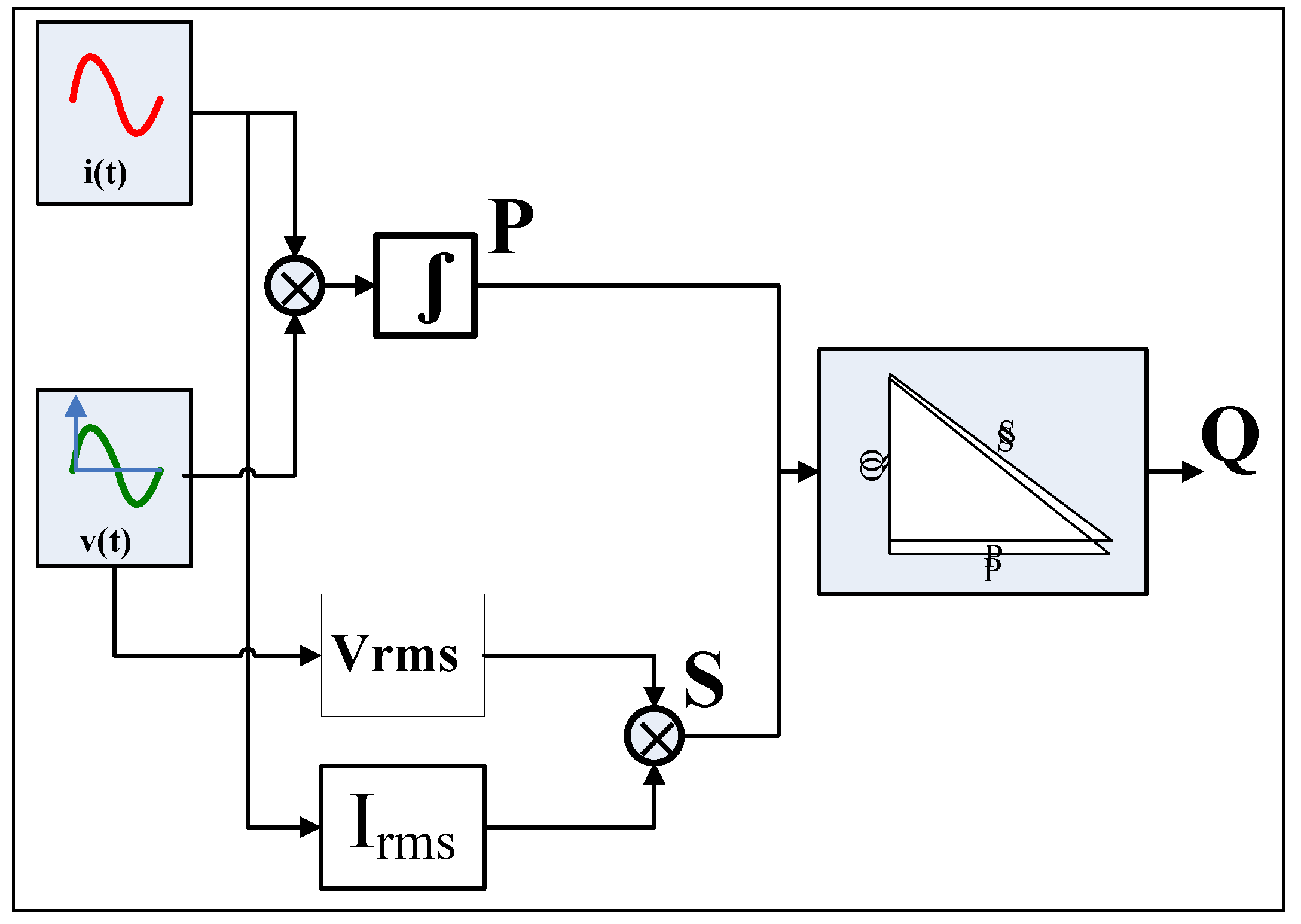
4. Reactive Power Measurement Using the DWT
This section covers the operating principles of the reactive energy meters using the power triangle method and the DWT. Let
v(
t) and
i(
t) be the time domain signal of the voltage and the current waveform, respectively. In the time domain, the rms value can be calculated as follows:
where
n is the total number of samples in one period of the waveform;
m is the current sample number; and
vm and
im are the voltage and current values, respectively, defined in the samples.
Using DWT, the rms value of the voltage and current waveforms can be expressed as follows:
where the
c’s and
d’s represent the scaling/approximation and detail wavelet coefficients; which quantify how closely the wavelet function matches the original waveform at sample time
k and frequency sub-band
j, with
jo as the lowest frequency sub-band; Subscripts
j and
k refer to the wavelet level/frequency sub-band and the sample time; respectively, while the superscripts
v and
i represent the voltage and current coefficients, respectively, in the wavelet domain. The apparent power at the approximation level (lowest frequency band)
jo,
Sjo, and the total apparent power
SDWT are as follows:
The reactive power in the wavelet can be calculated as:
where
PDWT, total active power, is the sum of approximations and detail active power and can be written as:
The reactive power
Q contains all the non-active power due to harmonics and any oscillating power that does not contribute to the power transmission. When considering the apparent power at the lowest wavelet decomposition, the reactive power becomes:
5. Implementation of the DWT
The wavelet theory was first applied to digital signal processing application following derivation of the PA for the DWT by Mallat [
24,
25]. Since then, many applications of the DWT have been explored. In recent years, DWT has become a powerful tool for analyzing and measuring power in energy meters. The DWT can be viewed as a multi-resolution decomposition of a sequence. The large-scale study of wavelets for power measurement in energy meters has pointed to the importance of practical implementation of power measurement using the DWT.
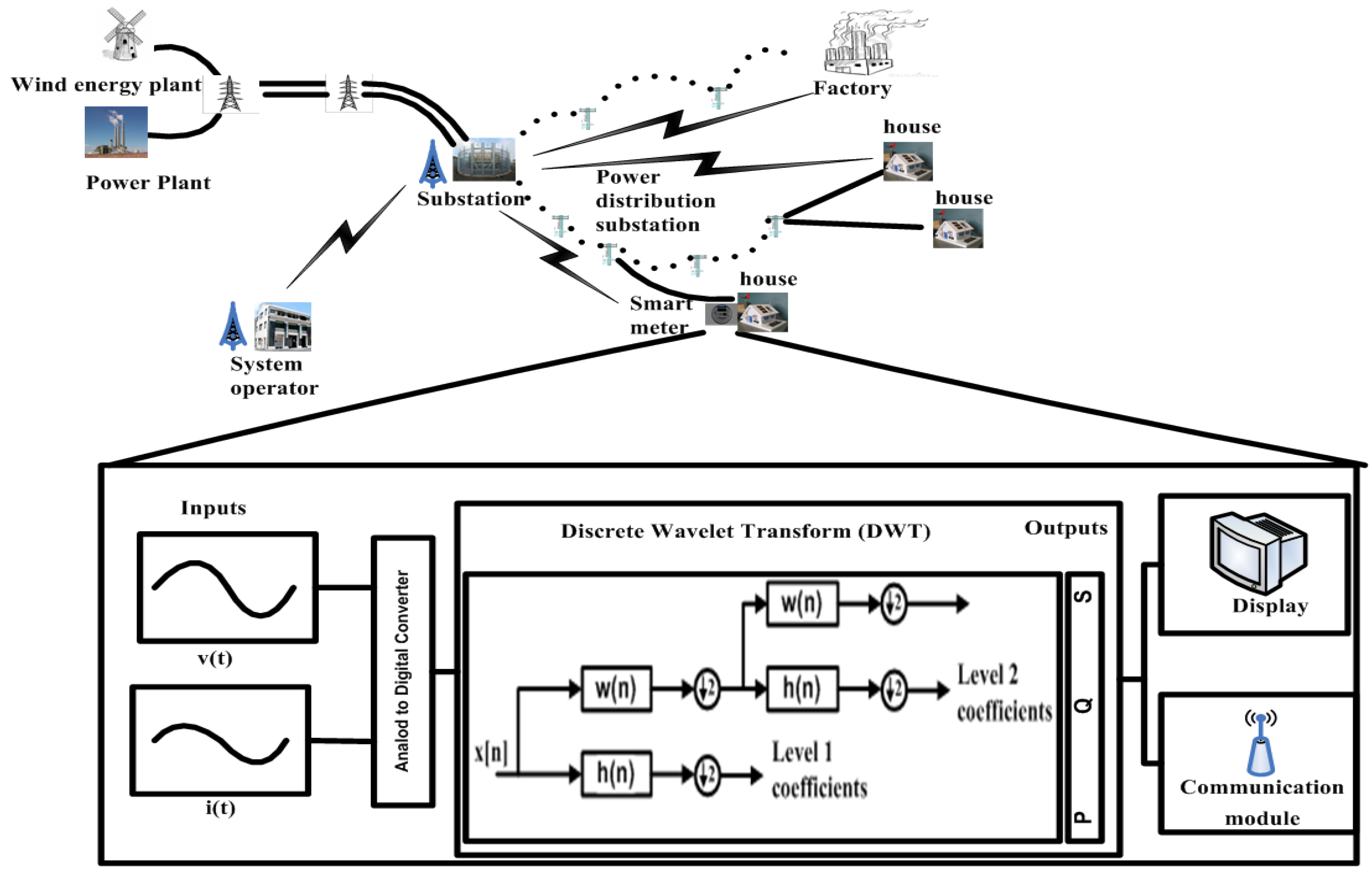
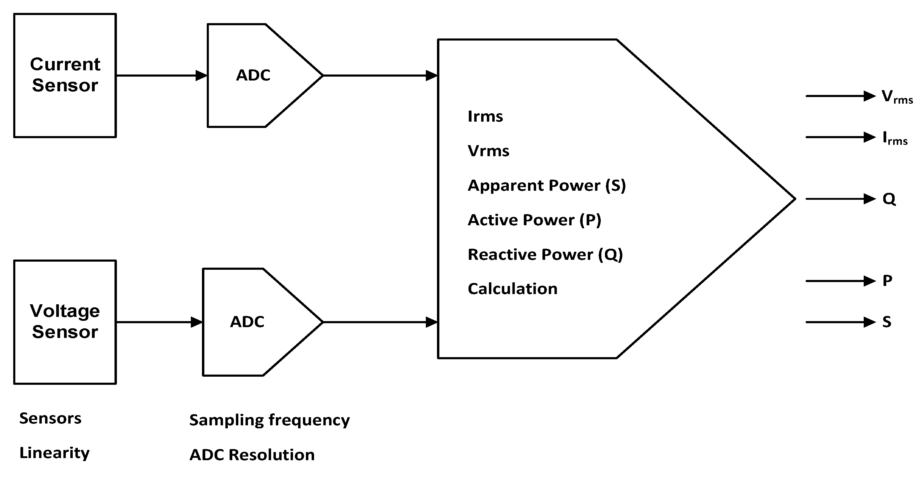
Figure 4 shows the block diagram of a smart meter in a smart grid, along with a schematic of the energy calculation algorithm using wavelet transform.
Figure 4.
Block diagram of an energy meter using wavelet transform in a smart grid.
Figure 4.
Block diagram of an energy meter using wavelet transform in a smart grid.
For
N points of input sequence
x(
n), DWT generates a sequence of length
N as the output
y(
n). The output has
N/2 values at the highest resolution and N/4 values at next to the highest resolution level, and so on. This mean time resolution is high at high frequency and low at low frequency, whereas frequency resolution is low at high frequency and high at low frequency. Let
N = 2
J, where
J is the number of frequencies. Therefore, the frequency index varies as 1, 2,…, J corresponding to the scales 2
1, 2
2,…, 2
J. The scaling and detailed wavelet coefficients can be computed as follows:
where:
| kth approximation and detail coefficient at level j; |
| w(),h() | Low pass and high pass L-tap filters obtained from chosen wavelet transform; |
| N-sample input signal x(n); |
| Number of wavelet coefficients in level j. |
The Pyramid Algorithm (PA)
The pseudo code for the Pyramid algorithm can be written as:
| Pyramid algorithm for N-point DWT computation |
begin c0(i) = x(i), i = 1,…N fs ← sampling rate a.TW ← observation interval for voltage or current waveform b. N = fs × TW J = log2N for (j = 1 to J) for (k = 1 to 2J − j) end for end for end for
|
where
J is the number of octaves;
N = 2
J is the length of sequence
x;
L is the length of the wavelet filter; and
w( ) and
h( ) are the low pass and high pass filters; respectively, derived from the wavelet. The output for the
jth octave is contained in
dj(
k)
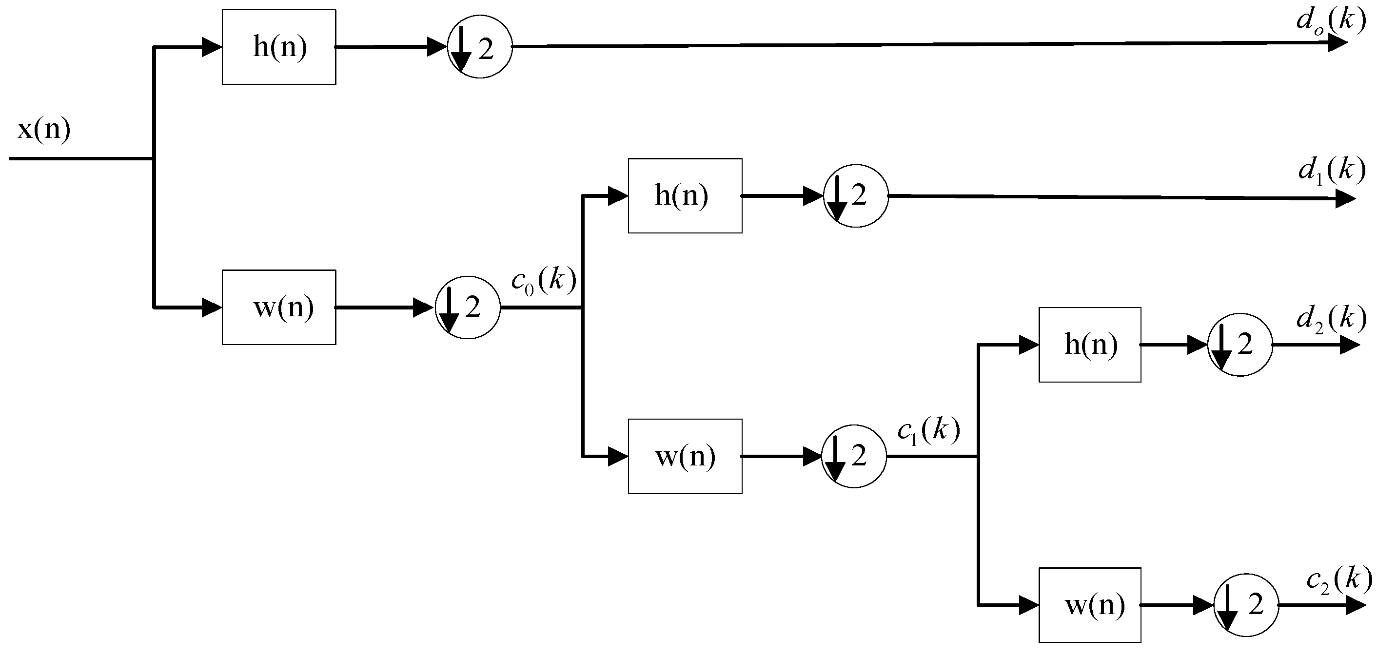
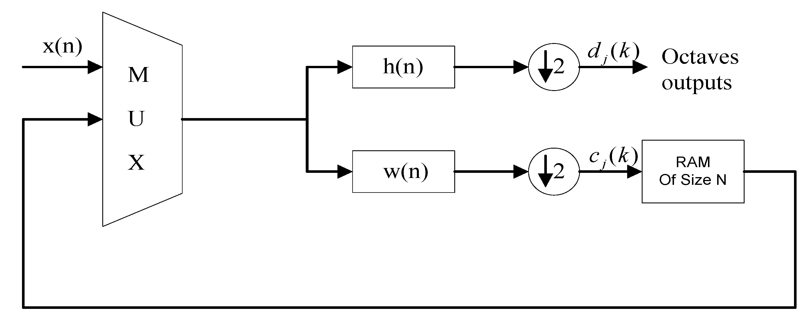
. The PA algorithm can be implemented using either filter bank architecture or folded architecture, as shown in
Figure 5 and
Figure 6, respectively.
Figure 5.
DWT filter bank architecture for J = 3 octaves.
Figure 5.
DWT filter bank architecture for J = 3 octaves.
Figure 6.
DWT folded architecture.
Figure 6.
DWT folded architecture.
Recursive Pyramid Algorithm (RPA)
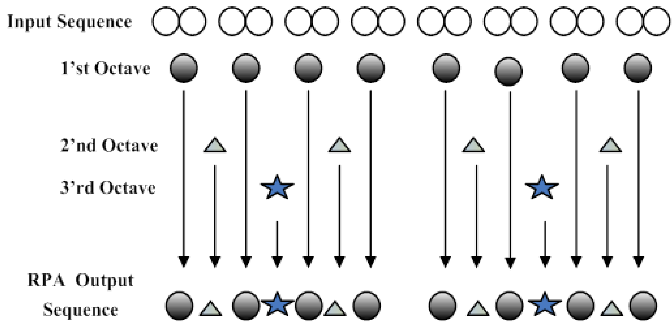
The RPA proposed by Vishwanth is a reformulation of the PA proposed by Mallat for real-time computation of the DWT coefficients. The core aim of the RPA is to make the memory size independent of the input length. The basic idea behind the RPA is to rearrange the computation order of the DWT coefficient. In the RPA, each coefficient computation is scheduled at the earliest possible instance. This schedule for computing the DWT coefficients is based on the precedence rule;
i.e., if the earliest instance of the
ith octave clashes with the (
I + 1)
th octave, then the
ith octave output is computed first. For the sake of understanding, the scheduling mechanism of the RPA considers a grid of the DWT coefficients as shown in
Figure 7. This is now pushed in a way that makes all horizontal lines line up in the form of a single line (RPA output sequence). The order of the output gives the output schedule. The advantages offered by the RPA are:
- ➢
Because each output of the jth octave is scheduled at the earliest instance, only the latest L words (L is the length of filter) need to be stored. Thus, the total memory size needed for DWT using RPA is L(J − 1), where J is the number of decomposition levels;
- ➢
The memory size can be small because each output of the different decomposition level is computed at the earliest possible instance. This removes the need to store the whole result of the jth octave for (j + 1)th octave computations;
- ➢
The input number of samples fed for each subsequent stage is equal to the length of the filter; therefore, it achieves a uniform rate; i.e., a practical rate.
Figure 7.
Scheduling diagram for the RPA.
Figure 7.
Scheduling diagram for the RPA.
The pseudo code for computing the N-point DWT using the RPA is as follows:
| Recursive Pyramid Algorithm for N-Point DWT Computation |
|
Function recursive_dwt (i, j)
begin if(i%2~=0) k = (i + 1)/2 else recursive_dwt (i/2, j + 1) end if end
|
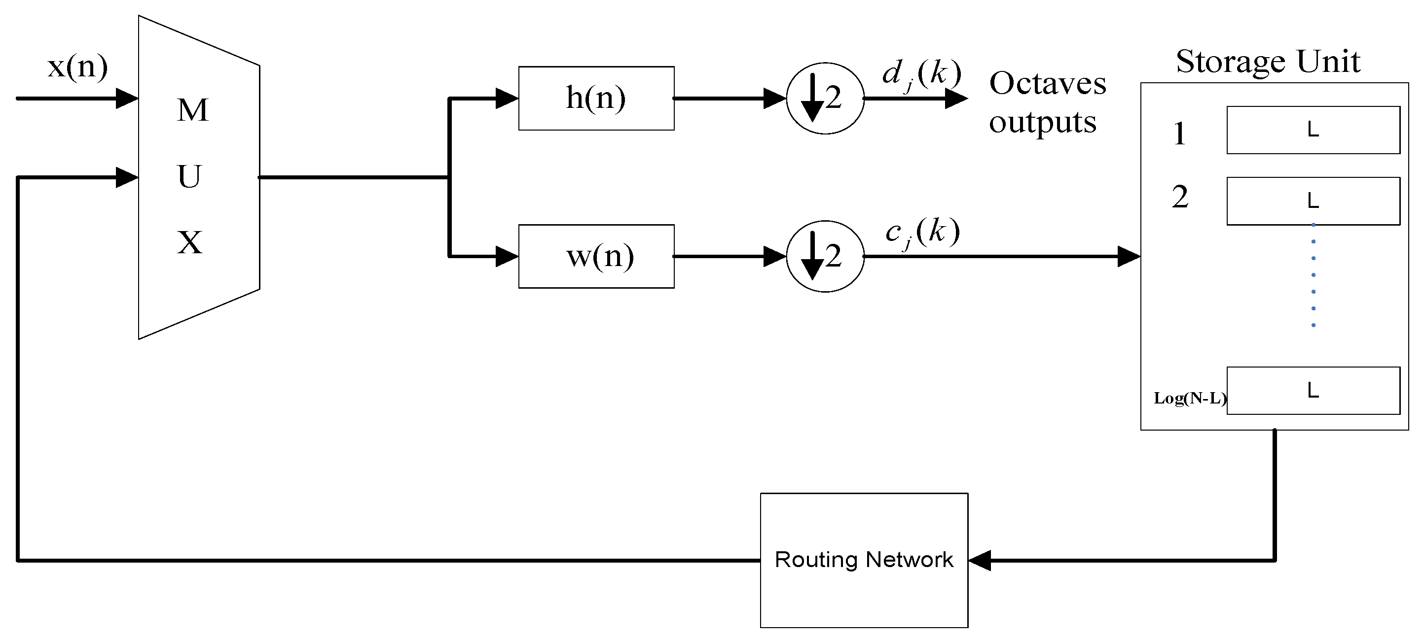
The RPA algorithm architecture is shown in
Figure 8. The routing network has to keep track of the latest Llog (N-L) blocks of output. The main disadvantage of implementing the RPA on general purpose computers is that the efforts required by the routing network to keep track of the latest Llog (N-L) block of output might prevail over the reduction in the memory storage because searching for data from a huge memory requires longer access time. Hence, smart meters can be implemented more practically using the DWT with the RPA, which requires fewer memory cells than the PA does.
Although, computing the DWT using the RPA reduces memory requirements quite remarkably, however, still it requires heavy arithmetic computation because it is essentially a two channel filter bank. This arithmetic complexity can be reduced by using lifting scheme implementation of the DWT [
28]. Implementation of lifting wavelet transform with an efficient RPA can be realized as an interesting future work for power measurement in smart meters.
Figure 8.
RPA implementation architecture.
Figure 8.
RPA implementation architecture.
6. Results and Discussion
This section first presents a comparison of the PA and the RPA in terms of the required numbers of memory cells and then provides an error analysis for power measurement using the DWT.
Table 2 shows the memory required for the PA and the RPA for an input sequence having different samples, with a filter having 20 and 40 samples.
Table 2.
Comparison of required numbers of memory cells for the pyramid algorithm (PA) and the recursive pyramid algorithm (RPA).
Table 2.
Comparison of required numbers of memory cells for the pyramid algorithm (PA) and the recursive pyramid algorithm (RPA).
| Input size (N) | Filter length (L) | Required memory cells PA (RPA) |
|---|
| 512 | 20 | 512 | 180 |
| 1024 | 20 | 1024 | 200 |
| 2048 | 20 | 2048 | 220 |
| 512 | 40 | 512 | 360 |
| 1024 | 40 | 1024 | 400 |
| 2048 | 40 | 2048 | 440 |
Two case studies are introduced for error analysis, considering sinusoidal (linear load) and non- sinusoidal (non-linear load) operating conditions to show the performance of power measurement using the DWT under varying parameters. The overall block diagram of the simulated system is shown in
Figure 9.
True values of the measurable quantities, such as
P,
Q, and
S, are already predetermined because the input voltage and current waveform are synthesized by known parameters. The true value of
Q is computed using the Hilbert transform. However, computing
Q using the Hilbert transform at reasonable cost is not practically feasible because it requires a dedicated processor to process the Hilbert transform necessary to compute a constant phase shift of 90° at each harmonic frequency [
29]. Hence, the value of
Q computed using the Hilbert transform approach is taken as the reference point and compared with the value of
Q computed using the DWT and the absolute error is presented in the results.
Figure 9.
Block diagram of the power measurement system.
Figure 9.
Block diagram of the power measurement system.
The input voltage or current waveforms are defined with parameters such as amplitude, fundamental frequency, and number of harmonics, phase offset, and (direct current) dc component.
The generalized form of sinusoidal voltage and current waveforms for case study 1 is defined as:
where
Vmax represents the peak voltage and
Imax is the peak current;
α is the amplitude scaling;
β is the dc offset;
γ is the phase offset and
t is the running time.
For the case study 2, the non-sinusoidal voltage waveform contains
n harmonics and can be expressed as:
These input waveforms pass through an analog to digital converter (ADC); two things are defined here:
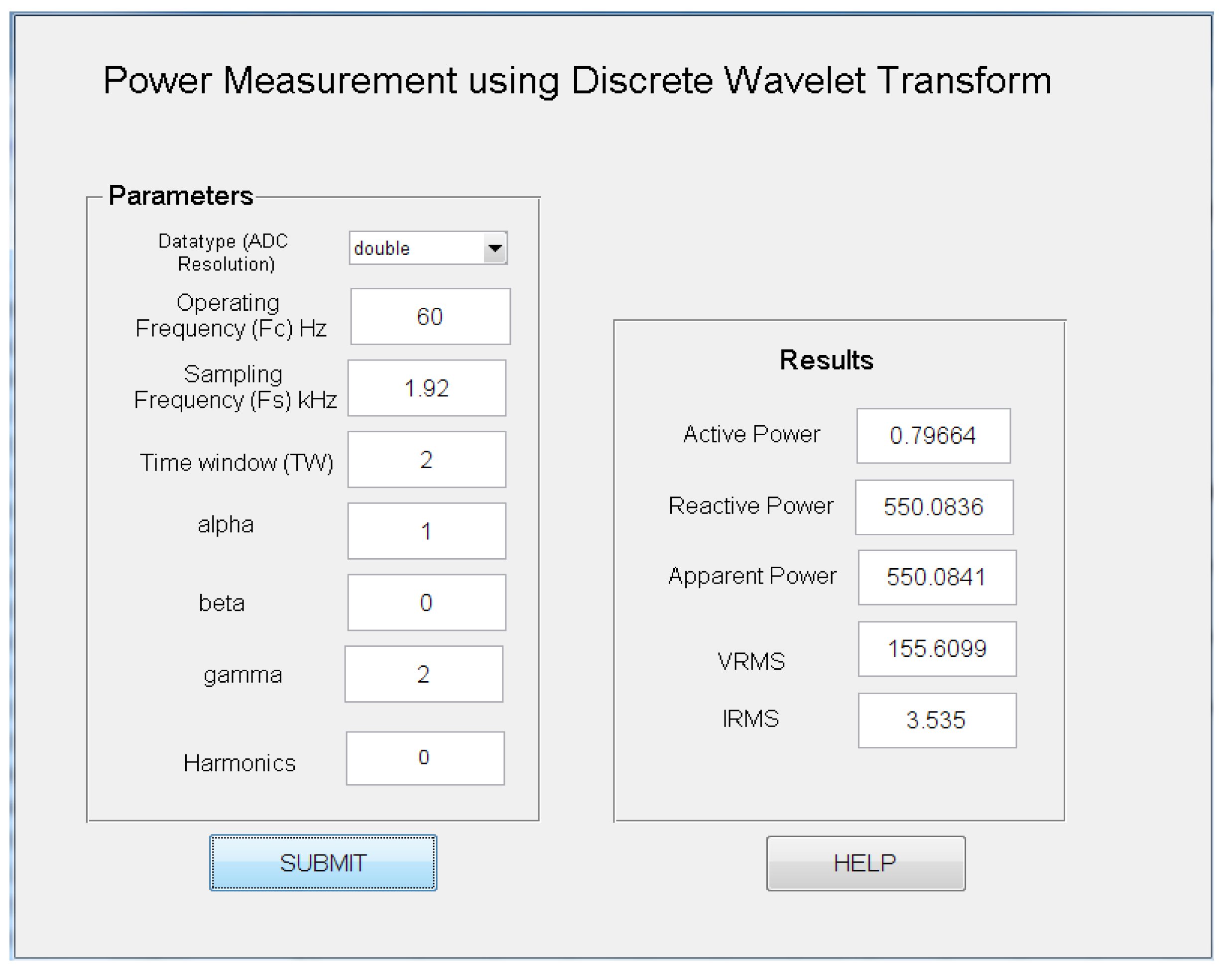
i.e., sampling rate and the ADC resolution, meaning how many bits a sample represents. These sample sequences are fed to the processing unit where the power calculation is performed using DWT. The mother wavelet chosen for the DWT is Daubechies 10 (db10) and Daubechies 20 (db20). The simulation is conducted in Matlab and the developed GUI interface is shown in
Figure 10. The time window (TW) in the figure indicates the observation time of the input waveform and is in multiple of the fundamental time period
T.
The impact of sensor linearity error is shown by varying α in Equation (16), the impact of DC offset is shown by varying β, the impact of phase offset is shown by varying γ, the impact of nonlinear load is shown by varying the number of harmonics, the effect of ADC resolution is shown by varying the number of bits used to store a sample, and the impact of sampling rate is shown by varying the sampling frequency fs.
Figure 10.
GUI for power measurement system.
Figure 10.
GUI for power measurement system.
Case study 1: Let both
v(
t) and
i(
t) be sinusoidal, with only a fundamental frequency component, and be given as:
The sampling frequency
fs is taken as 1.92 kHz and a 64 bit floating point numbering system is used. Various values obtained for
α,
β and
γ are shown in
Table 3. The values of
α,
β, and
γ for which the error value (ERR
Q) is lowest are highlighted.
Case study 2: Let
v(
t) be a waveform comprising three frequency components;
i.e., fundamental frequency, third, and fifth harmonic. Current
i(
t) contains just the fundamental frequency component. These are given as:
The sampling frequency
fs is taken as 1.92 kHz and a 64 bit (double) floating point numbering system is used. The results of varying values of
α,
β and
γ are shown in
Table 4. The values of
α,
β, and
γ for which the error value (ERR
Q) is lowest are highlighted.
Table 3.
Results for case study 1.
Table 3.
Results for case study 1.
| Mother wavelet | Inputs | Outputs |
|---|
| α | β | γ | Vrms | Irms | P | Q | S | ERRQ |
|---|
| db10 | 1 | 0 | 1 | 155.6099 | 3.5366 | 550.3285 | 0 | 550.3285 | 0 |
| 2 | 0 | 1 | 77.805 | 3.5366 | 275.1642 | 0 | 275.1642 | 0 |
| 1 | 0 | 2 | 155.6099 | 3.535 | 0.79664 | 550.0836 | 550.0841 | 0.0736 |
| 1 | 0 | 3 | 155.6099 | 3.5332 | 274.4743 | 476.3863 | 549.8001 | 0.0823 |
| 1 | 5 | 2 | 160.116 | 3.535 | 0.76768 | 566.0127 | 566.0132 | 16.013 |
| 1 | 10 | 2 | 164.6506 | 3.535 | 2.332 | 582.0384 | 582.0431 | 32.038 |
| db20 | 1 | 0 | 1 | 155.6099 | 3.5366 | 550.3285 | 0 | 550.3285 | 0 |
| 2 | 0 | 1 | 77.805 | 3.5366 | 275.1642 | 0 | 275.1642 | 0 |
| 1 | 0 | 2 | 156.5769 | 3.513 | 35.1974 | 549.3 | 550.0472 | 0.7 |
| 1 | 0 | 3 | 156.5769 | 3.4247 | 248.1128 | 475.3787 | 536.2321 | 0.37 |
| 1 | 5 | 3 | 156.4203 | 3.42427 | 247.6205 | 475.0306 | 535.6957 | 0.0306 |
| 1 | 10 | 3 | 156.4234 | 3.4247 | 247.1282 | 475.299 | 535.7065 | 0.299 |
Table 4.
Results for case study 2.
Table 4.
Results for case study 2.
| Mother wavelet | Inputs | Outputs |
|---|
| α | β | γ | Vrms | Irms | P | Q | S | ERRQ |
|---|
| db10 | 1 | 0 | 1 | 155.6146 | 3.53665 | 50.3335 | 3.54385 | 50.3449 | 3.5438 |
| 2 | 0 | 1 | 77.8128 | 3.53662 | 75.1692 | 3.54382 | 75.1921 | 3.5438 |
| 1 | 0 | 2 | 156.3219 | 3.535 | 1.2946 | 550.5994 | 552.6009 | 0.5994 |
| 1 | 0 | 3 | 156.3219 | 3.53322 | 277.5387 | 477.5193 | 552.3155 | 2.5193 |
| 1 | 5 | 2 | 160.8342 | 3.535 | 2.8589 | 568.5449 | 568.552 | 18.552 |
| 1 | 10 | 2 | 165.3746 | 3.535 | 4.4232 | 584.5856 | 584.6024 | 34.5856 |
| db20 | 1 | 0 | 1 | 155.6146 | 3.53665 | 50.3335 | 3.54385 | 50.3449 | 3.5438 |
| 2 | 0 | 1 | 77.8128 | 3.53662 | 75.1692 | 3.54382 | 75.1921 | 3.5438 |
| 1 | 0 | 2 | 157.33 | 3.513 | 1.29825 | 550.5186 | 552.5009 | 0.5186 |
| 1 | 0 | 3 | 157.33 | 3.4247 | 248.7419 | 477.4517 | 538.8113 | 2.45 |
| 1 | 5 | 2 | 157.1687 | 3.513 | 36.0938 | 550.9454 | 552.1264 | 0.9454 |
| 1 | 10 | 2 | 157.1664 | 3.513 | 36.1766 | 550.9318 | 552.1183 | 0.9318 |
The impact of ADC resolution on the power measurement is shown by conducting measurements under different data types;
i.e., double, int32, int16, and int8 for both the sinusoidal and non-sinusoidal cases under Daubechies 10 (db10). Let values of
α,
β, and
γ be 1, 0 and 2, respectively.
Table 5 shows the results for both case study 1 and case study 2.
Table 5.
Effect of ADC resolution on the power measurement.
Table 5.
Effect of ADC resolution on the power measurement.
| Data type | Case study 1 | Case study 2 |
|---|
| P | Q | S | ERRQ | P | Q | S | ERRQ |
|---|
| double | 0.79664 | 550.0836 | 550.0841 | 0.841 | 1.2982 | 550.5994 | 552.6009 | 0.5994 |
| int32 | 0.2737 | 572.9666 | 572.9667 | 22.966 | 2.2059 | 572.6717 | 572.6759 | 22.67 |
| int16 | 0.2737 | 572.9666 | 572.9667 | 22.966 | 2.2059 | 572.6717 | 572.6759 | 22.67 |
| int8 | 1.2933 | 404.0545 | 404.0566 | 146.05 | 0.09080 | 405.0339 | 405.0339 | 144.07 |
The impact of sampling frequency
fs on the power measurement is shown by conducting measurements under different sampling rates.
Table 6 shows the results for both case study 1 and case study 2.
Table 6.
Effect of sampling frequency on power measurement.
Table 6.
Effect of sampling frequency on power measurement.
| Samp Freq | Case study 1 | Case study 2 |
|---|
| fs (KHz) | P | Q | S | ERRQ | P | Q | S | ERRQ |
|---|
| 1.2 | 143.7319 | 529.1288 | 548.3029 | 1.6971 | 146.2492 | 530.9813 | 552.754 | 19.0187 |
| 1.6 | 89.0456 | 542.4225 | 548.6861 | 1.3139 | 91.6796 | 544.593 | 552.256 | 5.407 |
| 1.8 | 11.9928 | 549.9373 | 550.0841 | 0.841 | 14.1794 | 552.5994 | 552.5738 | 2.5994 |
| 1.92 | 0.79664 | 550.0836 | 550.068 | 0.68 | 1.2946 | 552.3919 | 552.6009 | 2.3919 |

