Saving Building Energy through Advanced Control Strategies

Department of Architectural Engineering, the Pennsylvania State University, University Park, PA 16802, USA
*
Author to whom correspondence should be addressed.
Energies 2013, 6(9), 4769-4785; https://doi.org/10.3390/en6094769
Submission received: 3 June 2013
/
Revised: 22 August 2013
/
Accepted: 2 September 2013
/
Published: 10 September 2013
(This article belongs to the Special Issue Energy Efficient Building Design 2013)
Abstract
:This article presents an analysis of the relationship between building energy usage and building control system operation and performance. A method is presented for estimating the energy saving potential of improvements in building and control system operation, including the relative impact of recommssioning and hardware and software upgrades, based on a subjective assessment of the level of energy efficient design and the energy usage of the building relative to similar buildings as indicated by the Energy Utilization Index for the building. The method introduces a Building Design Index and a Building Operating Index to evaluate building energy performance versus similar buildings, and uses these indices to estimate potential savings and effectiveness of control system improvements.
1. Introduction
The magnitude and relative importance of building energy consumption are well documented, clearly highlighting the potential benefits of techniques to improve building energy efficiency. The palette of possible approaches to do so includes many inter-related aspects, ranging from advanced materials, to improved components and intelligent systems. The process of designing, constructing and operating a building is a complicated one, with many actors, competing technologies, and potential pitfalls that can and do lead to suboptimal building performance in many instances. Poor building performance can be manifested in many ways as well, including inadequate indoor environmental conditions, excessive energy usage and cost, compromised equipment life, and a plethora of service calls. Many of these problems have a direct connection to the building control system, suggesting that improvements in building control system performance could result in substantial improvements in building utility.
It is a truism that time is money, and economic considerations will frequently result in less than complete attention to important building control system programming and commissioning activities. The nexus of this issue is that properly designing and implementing a building control system requires considerable expertise, since different buildings will have unique requirements and characteristics, and ultimately, different solutions. Beyond that, raising building control system performance to a level that can describe as optimal will generally require enhancing both hardware and software elements of the control system, frequently beyond the original design intent. At the current state of the industry, achieving optimal control is a time-consuming, expertise-laden exercise that is therefore costly and difficult. However, the expectation is that continuing advancements in intelligent control strategies will eventually result in solutions that can provide optimal control in a cost effective manner.
This paper will focus on two related issues relative to building control systems. The first is how to quantify the potential savings associated with improvements in building operation and control, while the second is how to actually achieve the savings in real buildings, particularly existing buildings, which represent the dominant target population.
2. Building Energy Usage and Control System Performance
There are two statements which are generally accepted a priori in the building industry, as follows:
- Buildings frequently use more energy than anticipated or desired;
- Building control system frequently do not operate properly.
There is an implicit assumption that these two statements are related in some way, which is certainly supported by both common sense and physics. Just as a vehicle’s fuel economy will suffer if the optimal operating conditions are not maintained, building energy efficiency will be subpar the operating conditions of all of the sub-systems are compromised. In the case of buildings, this represents an even greater challenge since buildings vary to a much greater extent than vehicles, meaning that many different and unique solutions may need to be developed and implemented. Also, the need to retrofit building systems is much more pervasive than that for vehicles.
Gaining accurate estimates of the energy saving potential of advanced building control systems requires information that is not easy to obtain, since the level of performance detail is beyond that which is normally monitored and collected. However, there have been a number of attempts to do so based on measurement and/or simulation, as described below.
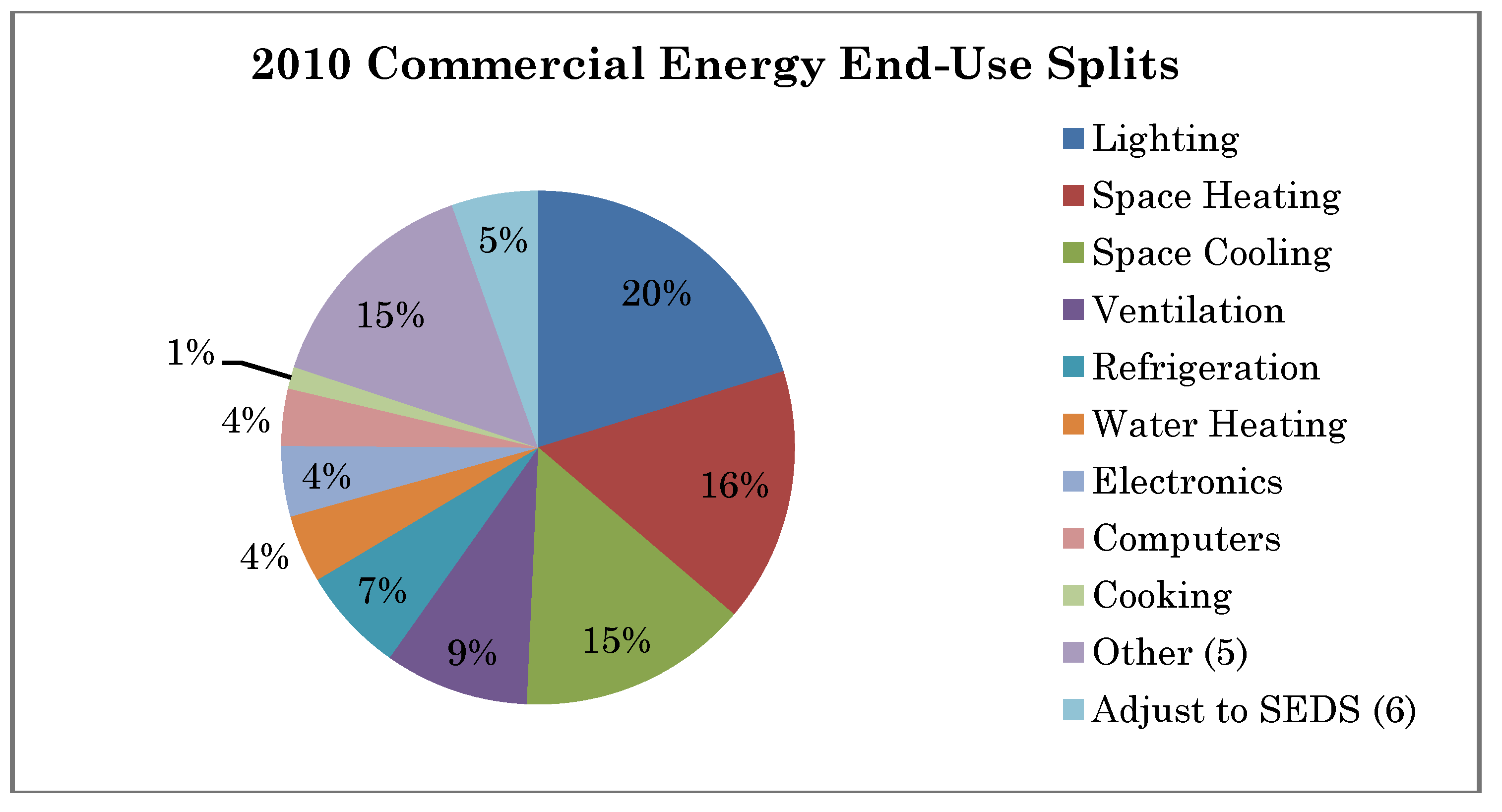
If we analyze the amount of energy consumed by each sector based on reported yearly energy data, (Figure 1) the energy end-use of commercial building are for lighting (20.2%), spacing heating (16.0%), spacing cooling (14.5%), ventilation (9.1%), refrigeration (6.6%), other (33.6%) based on primary energy [1]. These facts indicate about 60% of the energy end-use (i.e., lighting, space heating and cooling, ventilation) is somehow related to the building control system.
Figure 1.
Energy End-use split for commercial building in 2010 [1].
Figure 1.
Energy End-use split for commercial building in 2010 [1].

A number of studies indicated that optimal control strategies and fault diagnosis can reduce the energy waste and improve the overall building energy efficiency (see Table 1).

| References | Saving percentage | Study type |
|---|---|---|
| [2] | 25%–45% of energy used by HVAC system is wasted due to faults | Review |
| [3] | 4%–20% of energy consumed by HVAC, lighting, and larger refrigeration system in commercial building | Comprehensive review based on field data & survey |
| [4] | variable refrigerant flow air conditioning system can save 27.1%–57.9% energy compared to VAV AC system | Case study by simulation |
| [5] | Energy savings up to 30.4% were achieved during the summer season by using optimal setpoint control comparing with fixed temperature setpoint | Case study with simulation |
| [6] | The centralized and the distributed MPC strategies can reducing the energy consumption with 13.4% comparing to conventional P, PI, On/OFF control (for a selected day) | Case study with simulation |
| [7] | MPC with rule extraction for optimizing control sequences for window operation in mixed-mode building show the ability to save upwards of 40% of cooling energy through near-optimal night cooling strategies | Case study with EnergyPlus simulation |
Akinci, Garrett [2] summarized that 25%–45% of energy used by HVAC system are wasted due to faults, including improper control logic and strategy, malfunction of controllers and controlled devices, etc.
A comprehensive review by Roth et al. [3] identified and evaluated 13 key faults in commercial building. Based on date when the review was published, the total commercial building consumed approximately 17 quads of primary energy. The estimated likely range of the energy impact due to those faults could range from 0.24 to 1.8 quads, which was 2% to 11% of the total energy consumed by commercial buildings. The authors also concluded that those faults increase commercial building primary energy consumption by about 4% to 20% of energy consumed by HVAC, lighting, and larger refrigeration system in commercial building sector (i.e., approximately one quad) [3] (see Table 2).
Table 2.
The annual energy impact of faults selected for evaluation by Roth et al. [3].
| Fault | Fault type | By percentage | Annual energy consumption [quads] |
|---|---|---|---|
| Duct leakage | Air Distribution | 30% | 0.3 |
| HVAC left on when space unoccupied | HVAC | 20% | 0.2 |
| Lights left on when space un occupied | Lighting | 18% | 0.18 |
| Airflow not balanced | Air Distribution | 7% | 0.07 |
| Improper refrigerant change | Refrigeration Circuits | 7% | 0.07 |
| Dampers not working properly | Air Distribution | 6% | 0.055 |
| Insufficient evaporator airflow | Air Distribution | 4% | 0.035 |
| Improper controls setup/commissioning | Controls | 2% | 0.023 |
| Control component failure or degradation | Controls | 2% | 0.023 |
| Software programing error | Controls | 1% | 0.012 |
| Improper controls hardware installation | Controls | 1% | 0.010 |
| Air-cooled condenser fouling | Refrigeration Circuits | 1% | 0.008 |
| Valve leakage | Waterside Issues | 1% | 0.007 |
| Total | - | 100% | 1.0 |
Clearly, improved control system performance can reduce building energy consumption as well as improve the indoor environmental conditions. It is convenient to group the potential activities in this regard into three categories, as follows:
- Enabling or restoring control system operation to the design intent;
- Implementing conventional energy saving strategies such as economizer, energy recovery and set back;
- Adding advanced control capabilities such as model predictive or adaptive control.
Processes for dealing with each of these steps are detailed below.
2.1. Restoring to Design Intent
Achieving the first level of improvement generally requires a detailed examination of actual building HVAC and control system performance, along with a review of the control system specifications. This is sometimes called recommissioning, and requires quite a bit of hands on work verifying the proper operation of sensors and actuators, appropriate programming of the sequence of operation, and inspection of physical, electrical and mechanical components and systems.
If the control system is not operating properly as designed, energy usage could be either greater or less than anticipated, and space conditions could be out of tolerance. However, it is more likely that poor control system performance will result in excess energy usage since problems which result in less energy consumption will likely generate complaints from occupants regarding comfort conditions, and therefore be either fixed or otherwise ameliorated. Control problems that result in excess energy usage, such as simultaneous heating and cooling or over-ventilation, are likely to go undetected and will usually not result in complaints.
2.2. Implementing Conventional Energy Saving Strategies
Good practice, as well as contemporary building codes, dictate the utilization of certain energy saving strategies that might be termed conventional in the sense that they are commonly implemented and are frequently part of the control system vendor’s programming packages, making them relatively simple to incorporate. However, in addition to the software based features, the corresponding hardware capabilities are required to enable their utilization. The underlying configuration of the energy conversion and distribution systems must be amenable to the desired control strategies in order for them to be used, which may not always be the case. The most common missing elements are likely to be sensors, which is fortunate since they are somewhat easier to add without a great deal of cost or disruption. Additional actuators and flow control elements may also be needed, and these can prove to be more difficult and costly to retrofit. Substantially modifying HVAC system configuration can be very difficult and expensive, but is possible in many instances.
To the extent that some of the conventional energy saving strategies are not implemented, their addition can have a significant impact on energy consumption, the magnitude of the savings being a function of the specific building operating conditions.
2.3. Adding Advanced Control Strategies
The third and highest level of advanced control strategies generally are well beyond that which can be implemented using existing vendor software, and may also require hardware upgrades. Being currently the subject of numerous research activities, there is little standardization in their approach, implementation or operation. It is anticipated that in the near future, the more sophisticated algorithms and methods will be added as a higher level of hierarchical control using simulation models and numerical methods and communicating with the building control system via custom middleware or a network link. In the long run, it is hoped that the more successful approaches can be commercialized in a standardized fashion.
3. Building Control Systems, Energy Usage and Energy Savings
Stripped down to its most basic functionality, a building control system imposes setpoints and controls system components to maintain the desired interior environmental conditions, by turning things on and off, or modulating control signals to actuators or speed controls. Depending upon the sophistication of the control system, various sensor readings and programming logic will be used to cause the equipment and systems to operate in a prescribed manner as detailed in the design sequence of operation. For any given building HVAC system configuration and collection of components, if everything is operating properly, there will be a range of energy usages that would depend on how effectively the setpoints and control signals are managed by the control system, in response to the weather and occupant related issues. It has been shown that by taking careful consideration of the dynamic relationships between HVAC system components and the expected future course of weather and occupant driving forces, setpoints can be choreographed such that energy requirements are reduced compared to some other setpoint trajectory [8]. There is currently a great deal of interest in developing methods to determine the optimum set point trajectory for some set of conditions, using different aspects of model predictive control (MPC) [9,10,11]. There is a corresponding interest in assessing the effectiveness of the various MPC techniques, particularly their energy saving potential [6].
When trying to assess the potential energy savings from improving building control system operation, we inherently have to choose before and after scenarios. It can be imagined that if there is a building that wastes a lot of energy, there would be a lot of potential for improvement and consequent energy savings. Studies have shown that most if not all buildings exhibit some manifestation of sub-standard performance, ranging from faulty sensors and actuators, to heat transfer degradation, to improper or ineffective control logic, among other things. It can also be observed that the existing building stock, most of which has been around for decades, would represent a wide range of “energy efficient” design consciousness, with older or simpler buildings being less ambitious in utilizing high performance building design strategies. Thus, there could be some buildings that may be performing well, but use more energy because they lack the requisite energy saving materials, equipment and control capability, while other buildings which do have the energy saving features actually use excessive energy because of operating problems. The “fix” for the two above buildings is different. The building with the obsolete systems needs an upgrade, while the building with operating problems needs to be recommissioned. The recommissioning is not just for the control system, but for the entire building, including physical, mechanical and control system operation. This includes fixing envelope leaks, duct leaks, stuck/leaky valves and dampers, poor heat transfer, faulty sensors and improper control logic.
Figure 2 shows normalized building energy usage (NBE) at various stages of building design and operation for a simple building and a high performance building. The energy usage as designed is quite different for the two buildings, as would be expected and reflected in the As Designed bar graph. The As Built, before commissioning energy use would likely be much greater than the design values, and of a similar magnitude for the two buildings since the additional energy savings in the high performance building would not accrue without proper operation. Energy usage after the building is fully commissioned should be equal to the design intent, but over time, energy usage can increase as systems and components degrade, as shown in the figure. The potential energy savings for the two buildings at stage three are quite different in magnitude as well as in the activities required to attain the savings.
This suggests that we could represent the spectrum of building energy usage for a class of buildings as a function of the energy saving ambitiousness of the design and the degree to which the building is performing properly, that is in accordance with the design intent. It will be called the first dimension the Building Design Index (BDI), with the understanding that the term design refers specifically to energy efficiency. The second dimension then is Building Operating Index (BOI), again with the caveat that refers specifically to the aspects of building operation that are relevant to energy usage. Referring again to Figure 3, the BDI scale would represent the transition from simple to high performance building on a percentage basis defined by the difference between the two design intent bars. The BOI scale would represent the transition from poor to perfect building operation, with a value of 100% corresponding to design intent, and a value of zero corresponding to some designated amount of excessive energy usage not necessarily limited to the As Built energy usage, since there is the possibility of even worse energy performance.
Figure 2.
Normalized building energy usage at various stages of a building’s life.
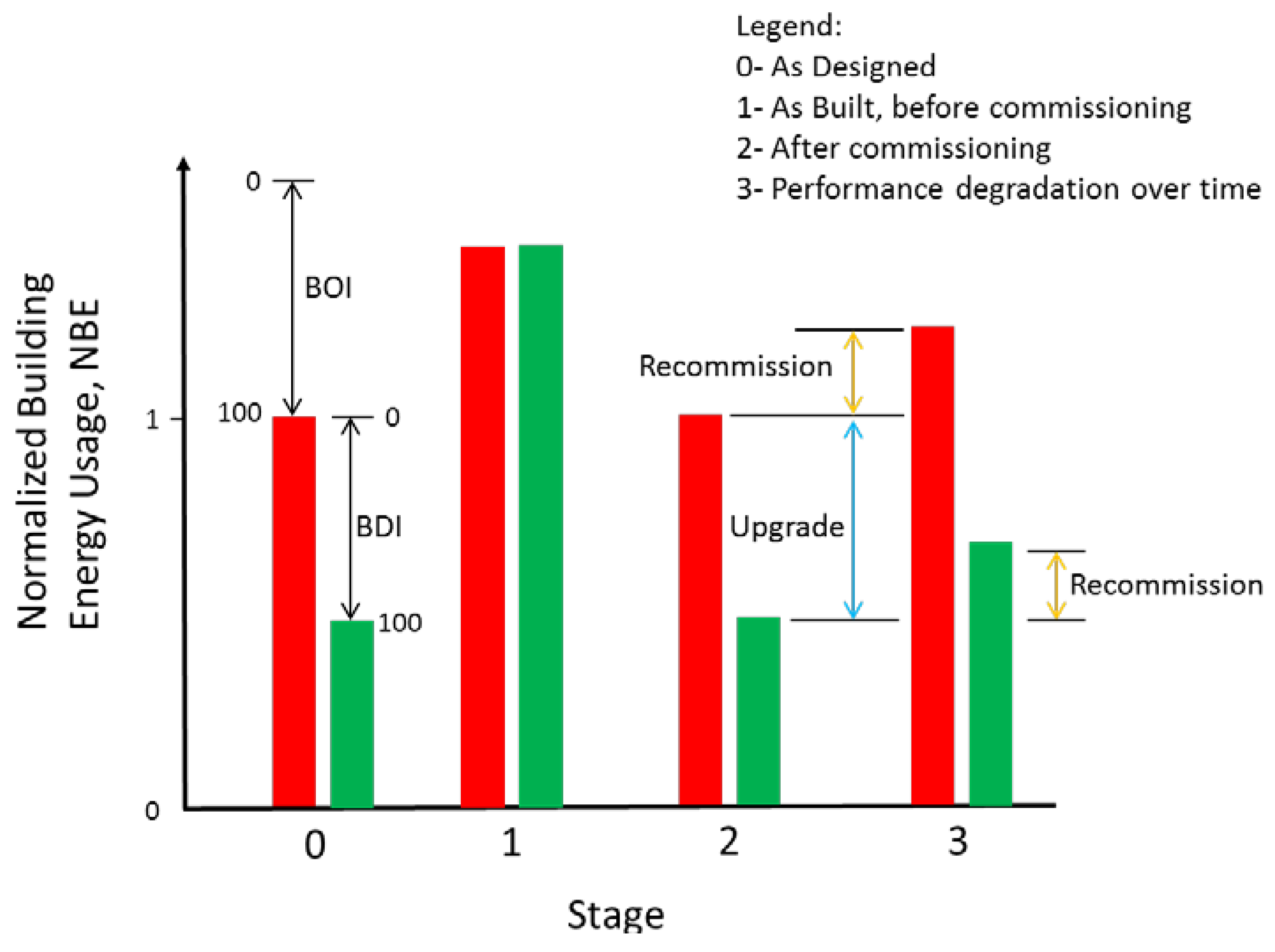
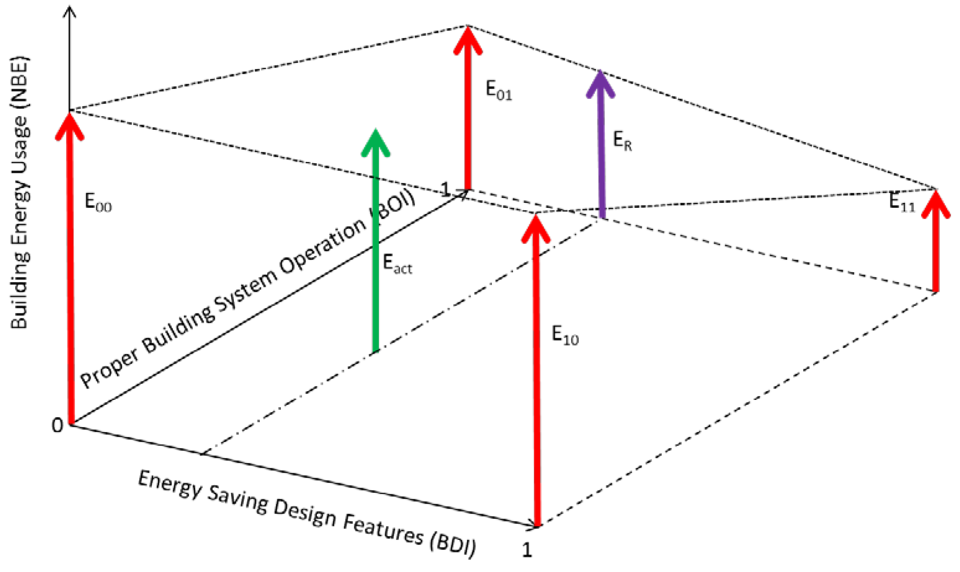
Figure 3.
Building Energy Usage as a function of design and operation indices.
Also shown in Figure 2, when a building has been in operation for some time, its energy usage can increase due to component and system degradation. Restoring a building to proper operation requires a comprehensive recommissioning, including physical, mechanical and logical aspects, which if completed could result in achieving a BOI value as high as 100%, while converting the simple building to a high performance building requires an extensive upgrade which could result in a BDI value of 100%.
This concept is shown in Figure 3. In this figure, the origin is in the lower left, which would represent a simple building which is not performing well. It should be noted that a BOI of zero does not mean the building is not operating at all, rather it is referring to the extreme low end of the possible range of operation. In contrast, a BDI of zero corresponds to a simple building with the default collection of basic operating functions. A BOI of one means that the building is operating perfectly as designed, but within its inherent limitations. A BDI of one in some respects represents an aspirational building, or at least a highly energy efficient building utilizing a comprehensive collection of high performance features.
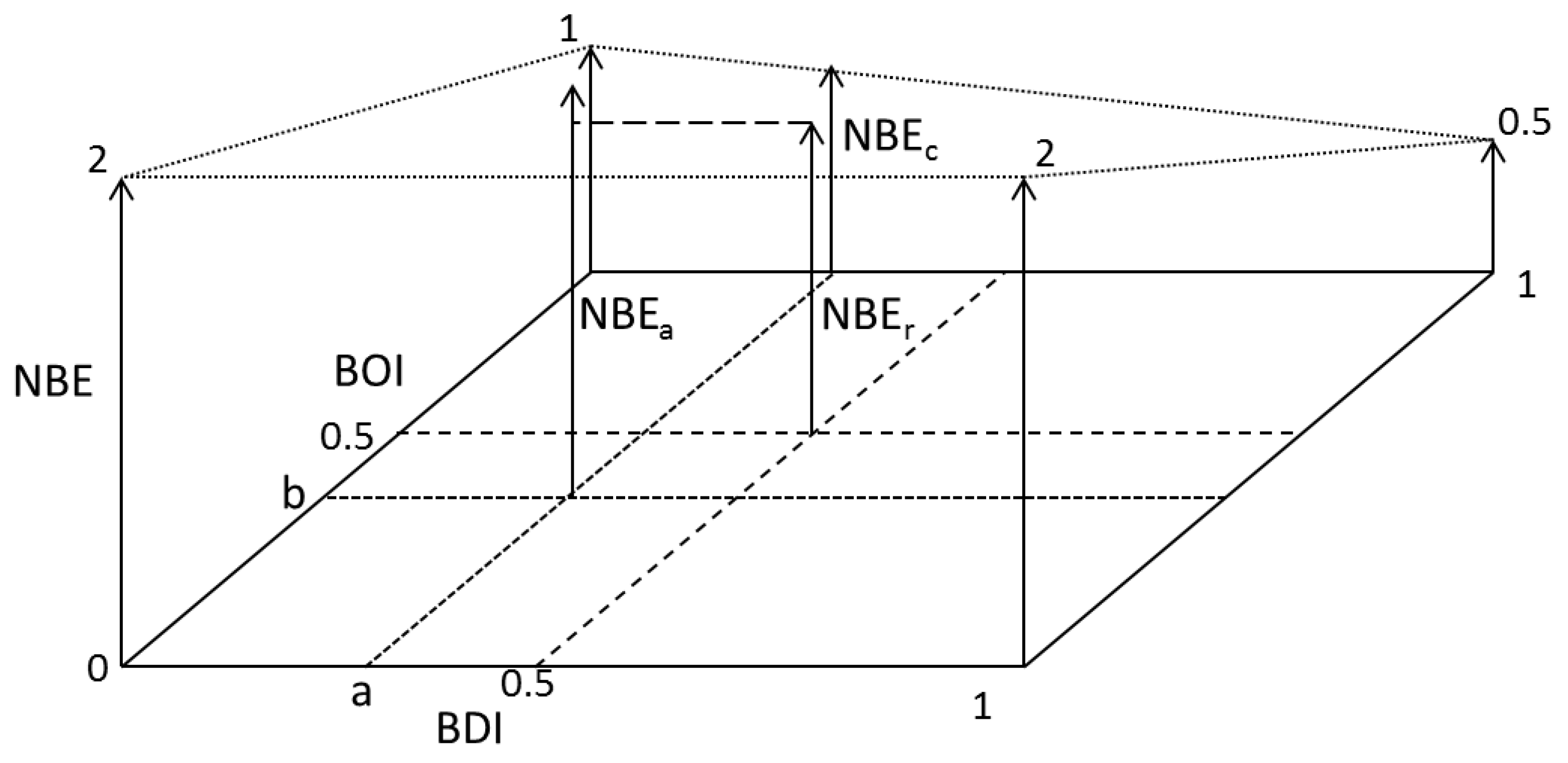
The method for determining the specific values for these two indexes will be addressed at a later point, but for now, the relevant information is represented by the arrows. The red arrows at the corners represent relative or normalized building energy usage (NBE). E00 is a simple, poorly performing building, E01 is the same building operating perfectly, E10 is the building completely upgraded but operating poorly, and E11 is the high performance building operating properly. It is safe to assume that building energy usage will decrease as building design and operation improve, and that buildings at intermediate values of either index would have corresponding intermediate energy usage values., with a surface shape as yet undefined. The rank ordering of E00, E01, and E11 clearly must descend, as first you fix the simple building and then you upgrade it and make sure all of the new systems are operating properly. It is also fair to assume that E10 will be nearly equal to E00, since the advanced features do not provide any benefit if they are not functioning, and may in some cases result in an increase in energy usage.
The green arrow represents the energy usage of the specific building of interest, Eact. The magnitude is known from energy bills (or simulations), but the location in the BDI-BOI space is not. If the BDI and BOI coordinates for the building of interest were known, potential energy savings due to recommissioning and upgrading could be estimated, as will be shown later. For the time being, let’s assume that we do know the BDI and BOI coordinates, as indicated by the location of the green arrow. The maximum energy saving potential due to both recommssioning and upgrading is the difference between Eact and E11. It is composed of two parts, namely the savings due to recommssioning, which is Eact minus ER which is the energy usage for the same BDI but a BOI of one, and the savings due to design upgrade, which is equal to ER minus E11. All of these values can be converted to percentage savings by dividing them by Eact.
At this juncture, three issues remain; one, how to determine the relative heights of the red arrows, two, what is the shape of the NBE surface spanning the coordinate space, and three, how to determine the specific values for BDI and BOI. Addressing these in order, a combination of approaches including heuristics, statistics and analytics was used to estimate the relative magnitudes of the corner arrows. If it starts with E01, the simple building that is operating perfectly, and assign that a relative energy usage value of one, it then needs to be decided how much more energy the building would use if it were operating poorly (E00), and how much less it would use if it received the benefit of a full high performance upgrade (E11). We can essentially define our BOI scale by selecting E00 to be some multiple of E01 such that extremely poor performance has been demonstrated. Intuition combined with a consideration of reported results suggests a factor of two might be reasonable in establishing a lower bound for the building operation scale. In other words, once building energy performance has degraded such that energy usage has doubled its design intent, the result is a BOI of zero. This does not imply that there might not be other buildings that may be in even worse operating condition, but an underlying assumption is that we are dealing with a population of buildings, however narrowly or broadly defined, that are generally similar. Thus, buildings which might be considered outliers would require special treatment. It will be also assumed that there is a linear relationship between NBE and BOI along the BOI axis, as shown by the dashed line connecting E00 and E01.
In the other dimension, E11 represents a slightly beyond-the-state-of-the-art building. Experience suggests that high performance buildings can be designed and operated to use less than half of the energy of a simple conventional building. This is also an aspirational target expressed by many in the building community. A linear relationship between NBE and BDI is assumed for BOI equal to one. So, the end result is factors of two in both directions, from two to one along the BOI axis, from one to one half along the back of the box, and a constant two along the BDI axis. Thus, the slope in the direction of BOI for BDI equal to one is the greatest of the four boundaries, as would be expected since getting all of the advanced features to work properly should provide a lot of improvement.
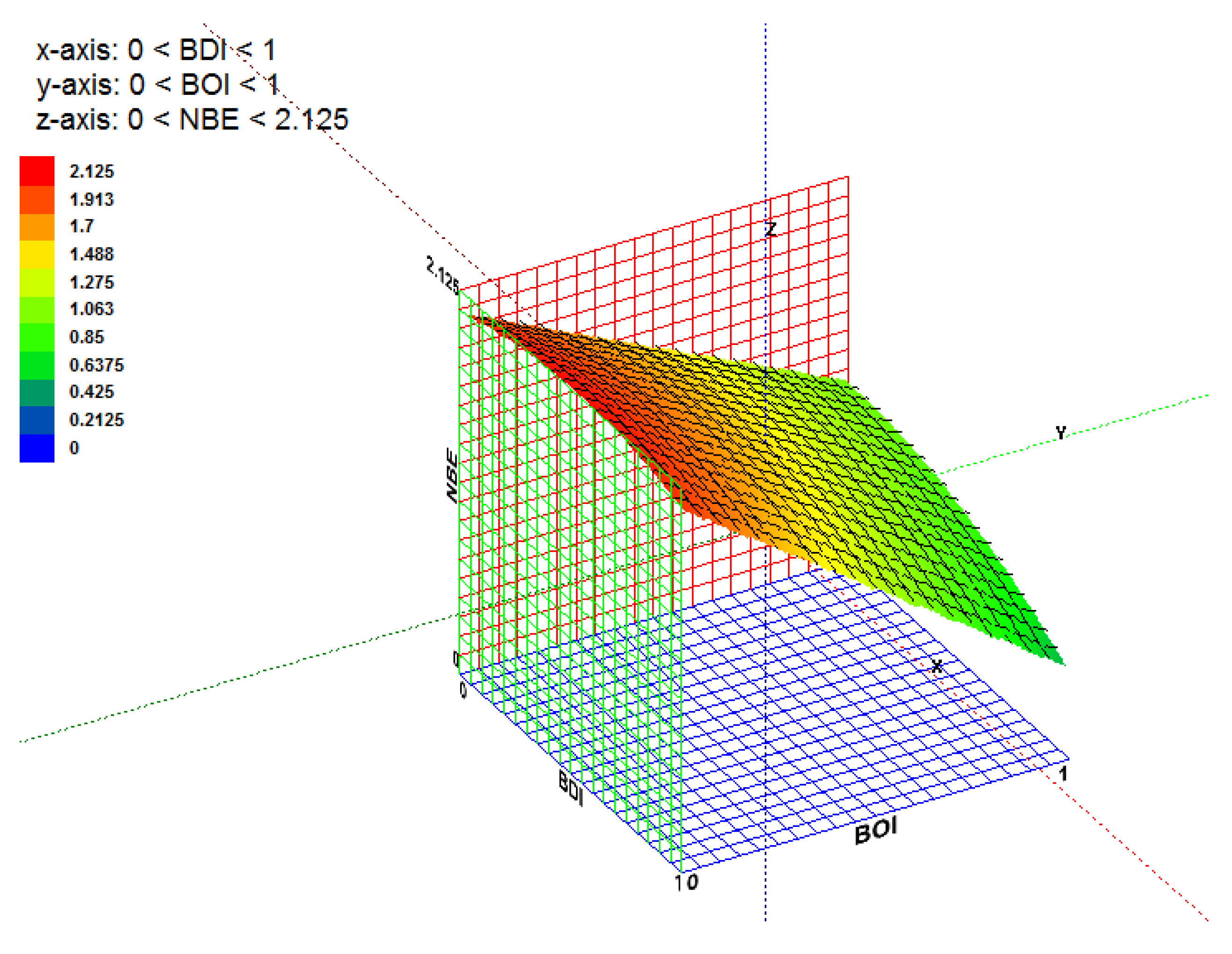
It should be noted that the analytical method described in the following can accommodate any relationship among the NBE values at the four corners, so that these could be customized based upon more specific information for a class of buildings. We would like to know the relative energy usage inside the BDI-BOI space, which requires the fitting of a surface to the boundary conditions as specified above. It can be assumed that the surface should be fairly smooth and well-behaved, so inspection suggests a quadratic form as follows:
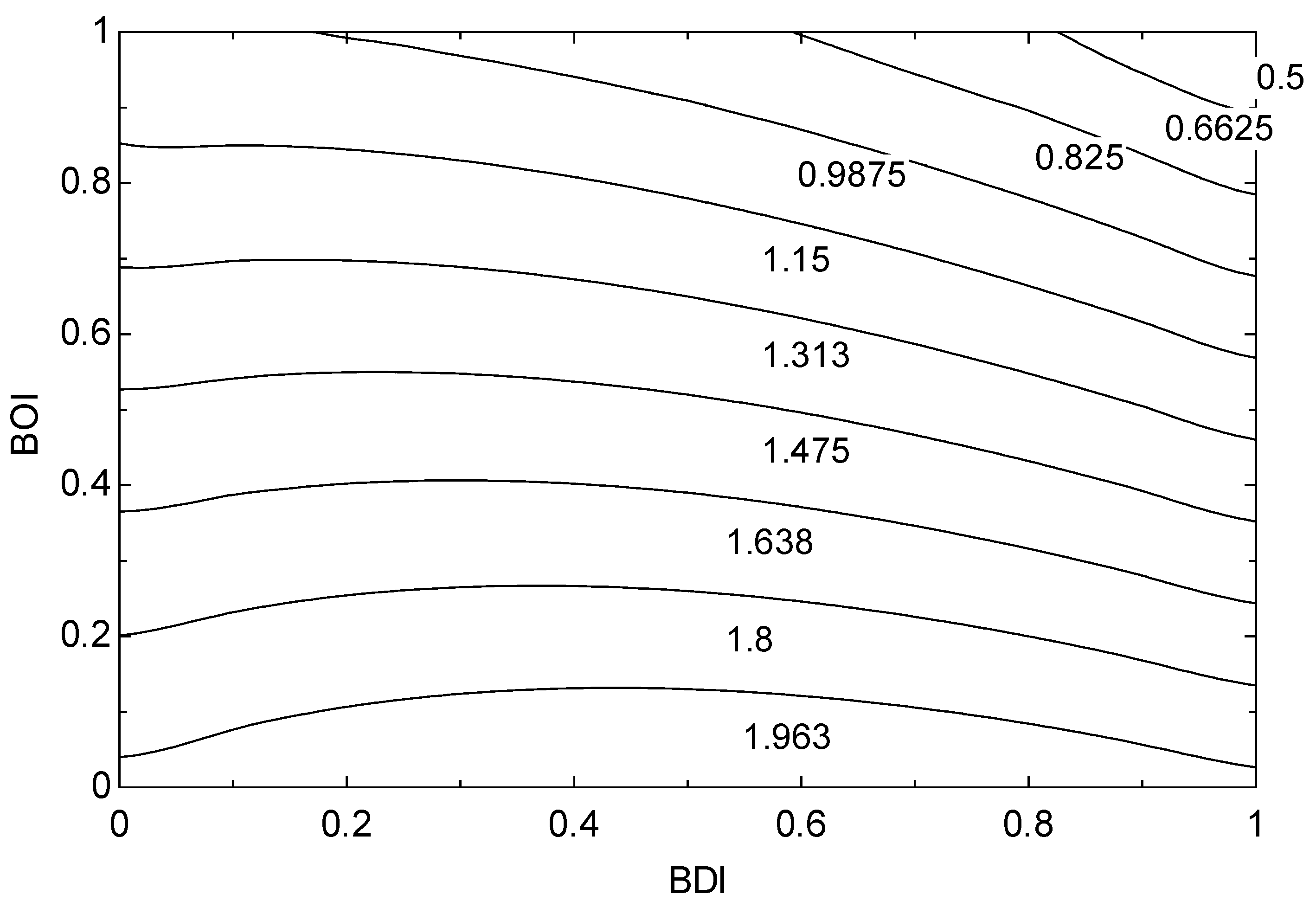
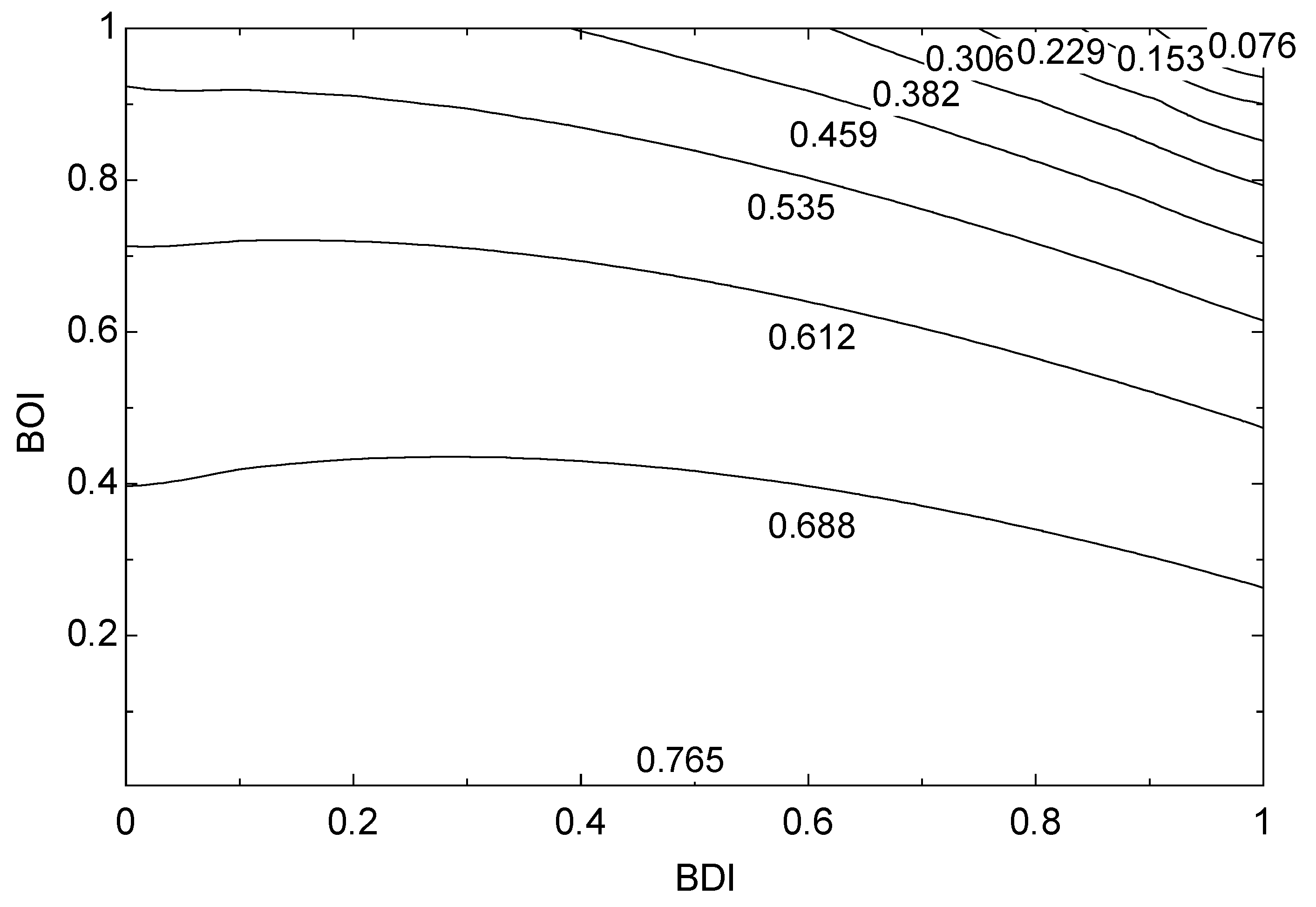
Using this equation, the relationship between NBE and the two indices can be plotted, as shown in Figure 4. This fits the corner points perfectly, and has a smooth transition across the space. There is a slight hump because the surface needs some curvature to match the boundaries. Figure 5 presents the surface information in the form of a contour plot.
Now that the NBE surface has been determined, it can be proceed with the method for determining the values of BDI and BOI for a specific building of interest. First, BDI is calculated based on a subjective assessment of the ambitiousness of the building and system design as regards energy usage. The subjective assessment uses semantic scaling, whereby someone knowledgeable about the building will rate the energy efficiency of the building and systems design in four categories, as follows:
- Building envelope and equipment
- Walls
- Insulation
- Roofs
- Fenestration
- Thermal, mechanical and electrical equipment
- Lighting
- Building systems configuration
- Constant or variable air volume
- Constant or variable water flow
- Heat pumps
- Ground source loops
- Building ventilation air
- Constant, scheduled, variable or demand controlled ventilation
- Economizer
- Energy recovery
- Dedicated outdoor air
- Building control capabilities
- Fixed setpoints
- Seasonal setpoints
- Scheduled setpoints, setback
- Real time dynamic setpoint adjustment
- Adaptive control
- Model predictive control
Figure 4.
Normalized Building Energy surface plot.

Figure 5.
Normalized building energy usage contours.

Now that the NBE surface has been determined, it can be proceed with the method for determining the values of BDI and BOI for a specific building of interest. First, BDI is calculated based on a subjective assessment of the ambitiousness of the building and system design as regards energy usage. The subjective assessment uses semantic scaling, whereby someone knowledgeable about the building will rate the energy efficiency of the building and systems design in four categories, as follows:
- 5.
- Building envelope and equipment
- Walls
- Insulation
- Roofs
- Fenestration
- Thermal, mechanical and electrical equipment
- Lighting
- 6.
- Building systems configuration
- Constant or variable air volume
- Constant or variable water flow
- Heat pumps
- Ground source loops
- 7.
- Building ventilation air
- Constant, scheduled, variable or demand controlled ventilation
- Economizer
- Energy recovery
- Dedicated outdoor air
- 8.
- Building control capabilities
- Fixed setpoints
- Seasonal setpoints
- Scheduled setpoints, setback
- Real time dynamic setpoint adjustment
- Adaptive control
- Model predictive control
Each of the categories has an individual weight such that they sum to 100%, and the subjective score in each category determines the credit earned. The semantic scale is shown in Table 3 and Table 4 outlines the BDI category weightings and default parameters.
| Score | Descriptive rating | Percentage credit |
|---|---|---|
| 0 | Default-old technology, basic | 0 |
| 1 | Minimal-slightly better | 10 |
| 2 | Modest-noticeably better, but below average | 25 |
| 3 | Typical-conventional commodity level | 50 |
| 4 | Above Average-clearly better, but not the best | 75 |
| 5 | Exceptional-maximum performance | 100 |
| Category | Weighting | Default parameters |
|---|---|---|
| Building envelope and equipment | 25 | Nearly obsolete or outdated |
| Building systems configuration | 25 | Constant air volume, dual duct, no special features |
| Building ventilation | 25 | Fixed outdoor air fraction |
| Building control capabilities | 25 | Fixed setpoints |
| Total | 100 |
The knowledgeable individual performing the assessment will use their expertise to gage where the building rates in each of the four categories, which determines the overall BDI. As shown in Figure 6, this confines the NBE for the building to a particular value of BDI, here indicated by the line labeled a. In order to determine where on the line it is located, the appropriate value for BOI must be determined. This is accomplished through the use of the parameter building Energy Utilization Index (EUI), which is simply annual total building energy usage divided by building floor area. This information is routinely collected, sorted and made available for many building classes and locations, and can be computed for the building of interest from energy bills. For this application, it would be useful to have EUI data for buildings of a class similar to the one of interest, if possible. For example, try to select an average EUI value for a similar type of building, at a similar location and climate. This should not be too difficult since EUI values are routinely compiled for various regions and building types [12]. The ratio of the EUI for the building of interest to the average EUI for that building class (and possibly size and location) is then computed. Since this is also the ratio of NBEa to NBEr, this uniquely determines the location of NBEa relative to the average building NBEr. By the definition of the BDI scale, an average building will have a BDI of 0.5. If it is assumed that the average building also has a BOI equal to 0.5, NBEr can be located at the center of the figure. Again, if we find information to support a different BOI value for the average building, that value can be used instead of 0.5. Referring again to Figure 6, it can be seen that NBEa now has a unique location at BDI = a and BOI = b. The maximum energy savings potential for the building would be NBEa minus 0.5 divided by NBEa, while the portion due to recommissioning would be NBEa minus NBEc divided by NBEa, with the balance being due to the update.
Figure 6.
Determining BOI from EUI ratio.

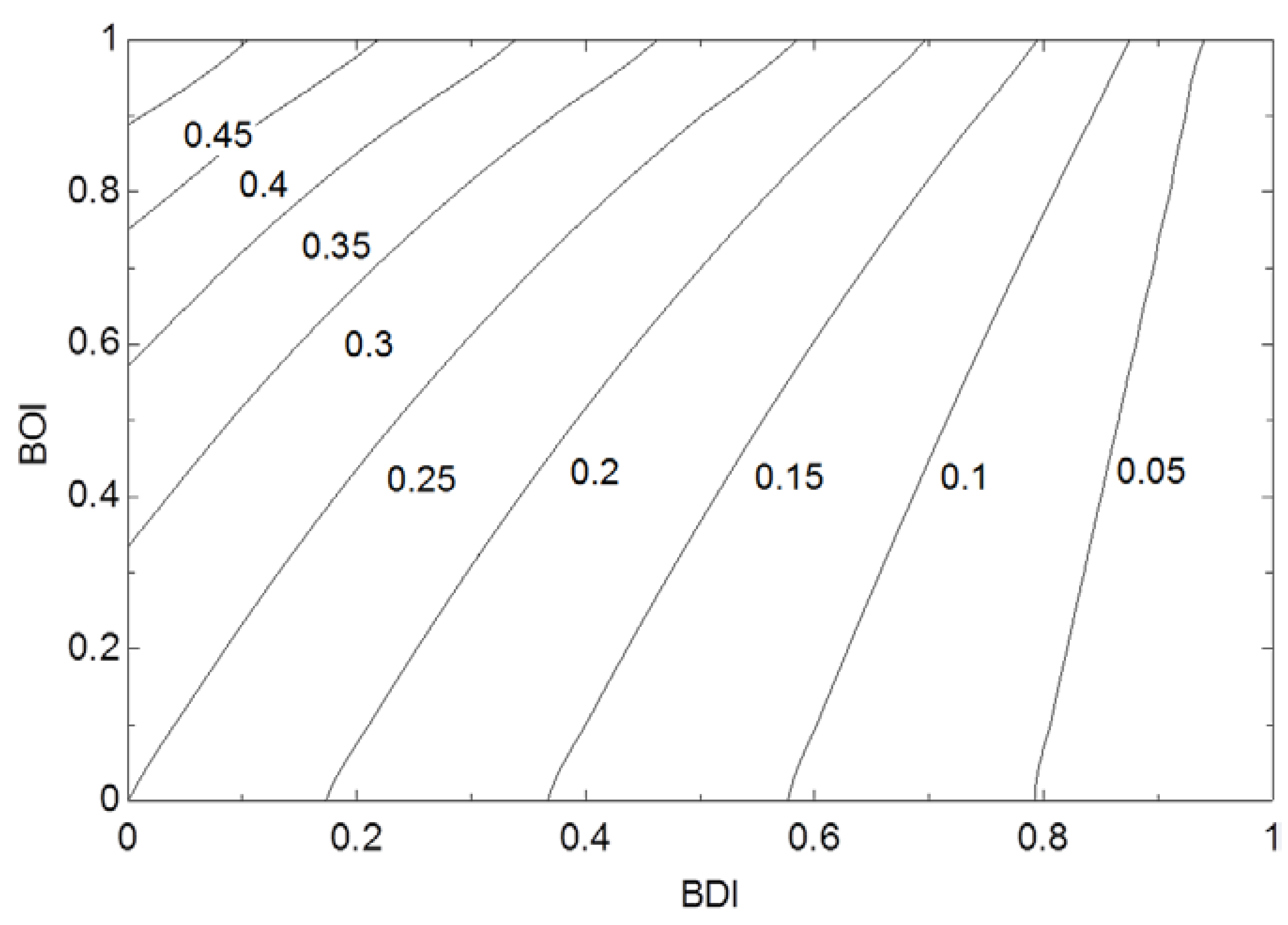
We can compute the maximum energy saving potential, the energy saving potential from recommissioning, and the energy saving potential from updating for any point in the BDI-BOI coordinate space, which are shown respectively in Figure 7, Figure 8 and Figure 9. The shapes of the contours are interesting, and reveal the relative insensitivity of potential energy savings through design improvements unless the building is operating with a BOI above 70%. Figure 7 indicates that the typical building located at BDI and BOI equal to 0.5 could expect a maximum energy savings of a little over 60%. Of course, in any building population there will be some variability in the performance characteristics of individual buildings. Some will benefit more from recommssioning, and others from updating, as can be seen in Figure 8 and Figure 9.
Figure 7.
Maximum building energy saving potential, ESPm.

Figure 8.
Building energy savings due to comprehensive recommissioning.
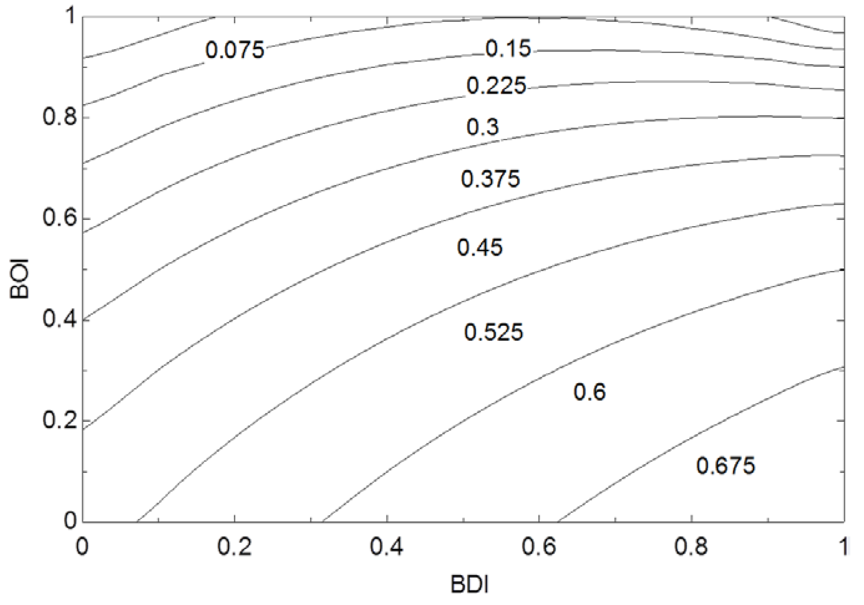
Figure 9.
Building energy savings due to upgrading only.
Before moving on, a few points bear further mention. First is the impact of fault detection and diagnosis (FDD). While FDD is usually considered an advanced control feature, it actual belongs with the building operation, and thus the BDI. FDD simply identifies performance problems which then need to be fixed. That is a facet of recommissioning. Second is the impact of renewable energy sources. Within the context of this analysis, renewables such as solar thermal, photovoltaic and wind energy belong with the other energy usage components, so should be added in to the EUI value for the building. Furthermore, if a building has some unusual energy usage components, particularly related to electrical energy for lighting or occupants, the building EUI should be adjusted to compensate by removing those components.
4. Discussion and Conclusions
For the existing building stock, generally, very little is known about how a specific building’s energy performance ranks across the spectrum of buildings. There are basically two areas where this methodology should prove useful if implemented.
- Assessing the energy performance of existing buildings relative to similar buildings or any collection of buildings, (i.e., community, city, region, etc.) as well as identifying how the energy performance is related to design versus operation. This information would be invaluable for a building owner to enable planning and prioritization of energy performance improvement activities such as recommissioning or upgrading, since improving operation and retrofitting are two distinct categories with different requirements and economic costs. Furthermore, the methodology could be used by a government agency or utility to assist in devising incentive programs to improve energy efficiency for a region or service area by enabling them to evaluate the status of the buildings and tailor their program to achieve the desired effects. Poorly performing buildings could be identified and targeted for improvement;
- Assessing the effectiveness of proposed or completed recommissioning or retrofit activities for a specific building by enabling the comparison of actual or predicted energy savings to maximum potential savings. In this manner, it would be possible to determine if additional measures are needed to reach the building’s full energy saving potential.
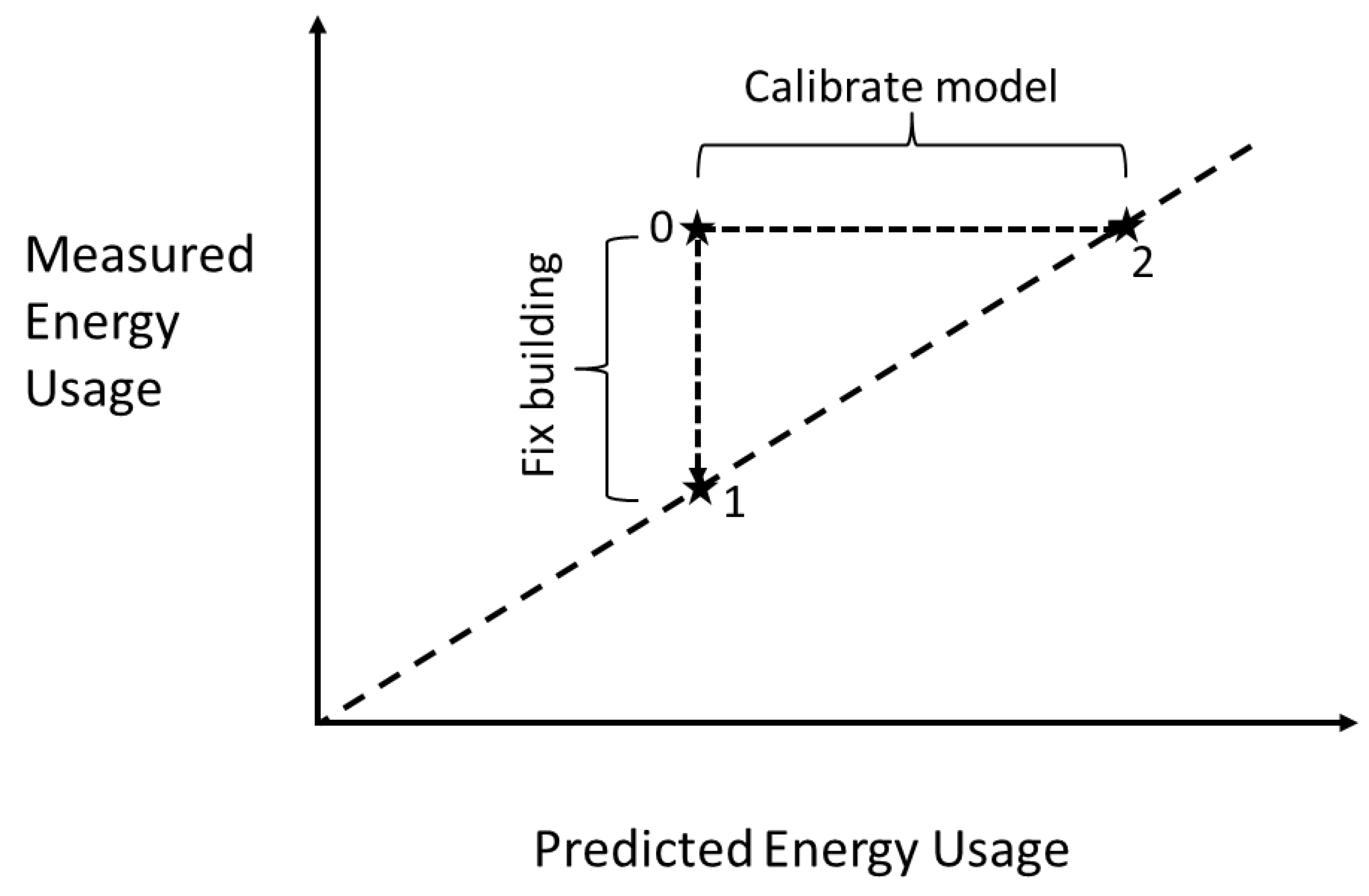
One of the biggest issues facing the building community is how to reduce building energy requirements while still meeting building comfort, health safety and productivity needs. Modeling and computer simulations have been used extensively to develop, refine and optimize building designs to achieve energy efficiency, but recent study has shown several issues related to model predictive control, one of which is prediction uncertainty [13]. It might result in disagreement between measured building energy usage and model predictions. There certainly are many possible reasons for the discrepancies, and the topic is too involved to extensively explore in this paper, but within the context of the method that has been outlined, some comments may prove useful. Referring to Figure 10, if we plotted measured versus predicted building energy usage, it would be expected the data points to fall on the diagonal dashed line if there were perfect agreement. However, in some cases, the building will use substantially more energy than predicted, particularly for the more ambitious, hence complicated, buildings. Such a point is designated in the figure as 0. The question is what steps should be taken when that occurs? Building energy usage can only be reduced by fixing the problems, which certainly involves recommissioning. There is a lot of interest in calibrating the building model, but that creates other issues. First, if the model is calibrated to the measured data, we then have a model for a poorly performing building, and have saved no energy. This is point 2 in the figure. Generally, the model cannot be used to find the problems; rather, it needs to find the problems to fix the model, resulting in a model which has little usefulness. Second, in the process of calibrating the model, we have to learn a great deal about how the building is actually operating, flaws and all, and then somehow incorporate them in the model. The exercise of identifying the building flaws is also the first step towards fixing the building, which will actually allow energy to be saved. This is point 1 in the figure. So in terms of time well spent, it is better to identify the operational problems with the building and fix them, and then use the model for the properly functioning building to make predictions for control. The benefit of the advanced control and operating features can only be obtained when they are present and the building is operating properly.
To wrap up the discussion, an additional metric of interest is how effective a particular advanced control strategy is. It has been seen that energy savings is a moving target that depends on both the before and after performance values as well as the ultimate savings potential. We can define Energy Savings Effectiveness (ESE) as the ratio of energy savings actually achieved to the maximum energy savings potential (ESPm) for the building of interest. Once the building BDI and BOI are determined, Figure 7 can be used to determine ESPm, allowing the ratio to be computed using the actual or predicted savings. For example, for the hypothetical average building, ESPm is about 67%, with 50% being due to recommissioning and 17% being due to updating. So if a particular advanced control strategy saves 15%, that would be an ESE of 22%, but it would also have captured 88% of the potential savings due to updating.
Figure 10.
Measured vs. Predicted Building Energy Usage.

Conflicts of Interest
The authors declare no conflict of interest.
References
- U.S. Department of Energy (DOE). 3.1.4. 2010 Commercial Energy End-Use Splits, by Fuel Type (Quadrillion Btu). In Building Energy Data Book; U.S. DOE: Washington, DC, USA, 2010. [Google Scholar]
- Akinci, B.; Garrett, J.H.; Akin, Ö. Identification of Functional Requirements and Possible Approaches for Self-Configuring Intelligent Building Systems; National Institute of Standards and Technology: Gaithersburg, MD, USA, 2011. [Google Scholar]
- Roth, K.W.; Westphalen, D.; Feng, M.Y.; Llana, P.; Quartararo, L. Energy Impact of Commercial Building Controls and Performance Diagnostics: Market Characterization, Energy Impact of Building Faults and Energy Savings Potential; A Report for Building Technologies Program: Cambridge, MA, USA, 2005. [Google Scholar]
- Aynur, T.N.; Hwang, Y.H.; Radermacher, R. Simulation comparison of VAV and VRF air conditioning systems in an existing building for the cooling season. Energy Build. 2009, 41, 1143–1150. [Google Scholar] [CrossRef]
- Mossolly, M.; Ghali, K.; Ghaddar, N. Optimal control strategy for a multi-zone air conditioning system using a genetic algorithm. Energy 2009, 34, 58–66. [Google Scholar] [CrossRef]
- Moroşan, P.D.; Bourdais, R.; Dumur, D.; Buisson, J. Building temperature regulation using a distributed model predictive control. Energy Build. 2010, 42, 1445–1452. [Google Scholar] [CrossRef]
- May-Ostendorp, P.; Henze, G.P.; Corbin, C.D.; Rajagopalan, B.; Felsmann, C. Model-predictive control of mixed-mode buildings with rule extraction. Build. Environ. 2011, 46, 428–437. [Google Scholar] [CrossRef]
- Hazyuk, I.; Ghiaus, C.; Penhouet, D. Optimal temperature control of intermittently heated buildings using model predictive control: Part II—Control algorithm. Build. Environ. 2012, 51, 388–394. [Google Scholar] [CrossRef]
- Ma, Y.; Anderson, G.; Borrelli, F. A Distributed Predictive Control Approach to Building Temperature Regulation. In Proceedings of the 2011 American Control Conference (ACC), San Francisco, CA, USA, 29 June–1 July 2011; pp. 2089–2094.
- Široký, J.; Oldewurtel, F.; Cigler, J.; Prívara, S. Experimental analysis of model predictive control for an energy efficient building heating system. Appl. Energy 2011, 88, 3079–3087. [Google Scholar] [CrossRef]
- Oldewurtel, F.; Parisio, A.; Jones, C.N.; Morari, M.; Gyalistras, D.; Gwerder, M.; Stauch, V.; Lehmann, B.; Wirth, K. Energy Efficient Building Climate Control Using Stochastic Model Predictive Control and Weather Predictions. In Proceedings of the 2010 IEEE American Control Conference (ACC), Baltimore, MD, USA, 20 June–2 July 2010; pp. 5100–5105.
- Commercial Buildings Energy Consumption Survey (CBECS); U.S. Department of Energy, Energy Information Administration: Washington, DC, USA, 2003.
- Ma, Y.; Kelman, A.; Daly, A.; Borrelli, F. Predictive control for energy efficient buildings with thermal storage: Modeling, stimulation, and experiments. IEEE Control Syst. 2012, 32, 44–64. [Google Scholar] [CrossRef]
© 2013 by the authors; licensee MDPI, Basel, Switzerland. This article is an open access article distributed under the terms and conditions of the Creative Commons Attribution license (http://creativecommons.org/licenses/by/3.0/).
Share and Cite
MDPI and ACS Style
Treado, S.; Chen, Y. Saving Building Energy through Advanced Control Strategies. Energies 2013, 6, 4769-4785. https://doi.org/10.3390/en6094769
AMA Style
Treado S, Chen Y. Saving Building Energy through Advanced Control Strategies. Energies. 2013; 6(9):4769-4785. https://doi.org/10.3390/en6094769
Chicago/Turabian StyleTreado, Stephen, and Yan Chen. 2013. "Saving Building Energy through Advanced Control Strategies" Energies 6, no. 9: 4769-4785. https://doi.org/10.3390/en6094769