1. Introduction
Inter-area electromechanical oscillation has been one of the most severe threats for the safe and economic operation of modern power systems [
1,
2] due to the increasing large interconnection of power grids. Most investigations show that the local measurement-based power system stabilizer (LPSS) is effective in damping local oscillation modes, but its effectiveness in damping inter-area mode oscillations is limited [
3]. As the smart grid has been developed, the applications of WAMS via phasor measurement unit (PMU) have influenced the future of development of advanced technique implemented in electrical power engineering. The WAMS will be a solution of the smart grid implementation, and WAMS for smart grid applications involves the power system measurement, monitoring, protection and control [
4,
5,
6,
7,
8]. Thanks to the WAMS and the development of smart grids, many remote signals-based PSSs have been designed to suppress inter-area oscillation modes [
8].
Via synchronized signals from WAMS, a coupled vibration model based on the exact model of power system is well suited for off-line designs, while little information could be provided to on-site operators. Instead, online approaches, such as Prony [
9] and H
∞ [
10] analysis, have recently been presented to conduct online inter-area electromechanical oscillation parameter extraction and damping control. Nevertheless, the signal time delay between the instant of measurement and that of the signal being available to the controller, would deteriorate the control performance of the remote signals-based power system stabilizer (PSS) [
3,
10]. As time delay in WAMS is usually obvious, it should be accounted for to consider its impact on the remote signals-based PSS design in smart grids. In order to compensate the various time delays, the linear matrix inequality (LMI) [
11,
12] and H
∞ [
13,
14] methods could be employed to design the PSS. In these methods, complex treatment of time delays would not only increase the processing time but also reduce the practicability of wide-area damping control.
For the fast-development of smart grids, this paper presents a novel adaptive wide-area control scheme in which: (a) the subspace identification technique (SIT) is adopted to derive the linear model of power system, identify inter-area oscillation modes and calculate the measurement-based participation factor; (b) the control signals and the generators which need to be supplemented by wide area control information are determined; (c) the wide-area damping controllers (WADCs) with their parameters derived adaptively for PSS are constructed; and (d) a simple but practical time delay compensator is designed to eliminate the effects of signal transmission time delay. Simulations on the IEEE test system under various disturbance scenarios have validated that the presented adaptive wide-area control scheme for damping inter-area oscillation is effective and robust.
2. Design of Adaptive WADC for Remote Signal Based PSS
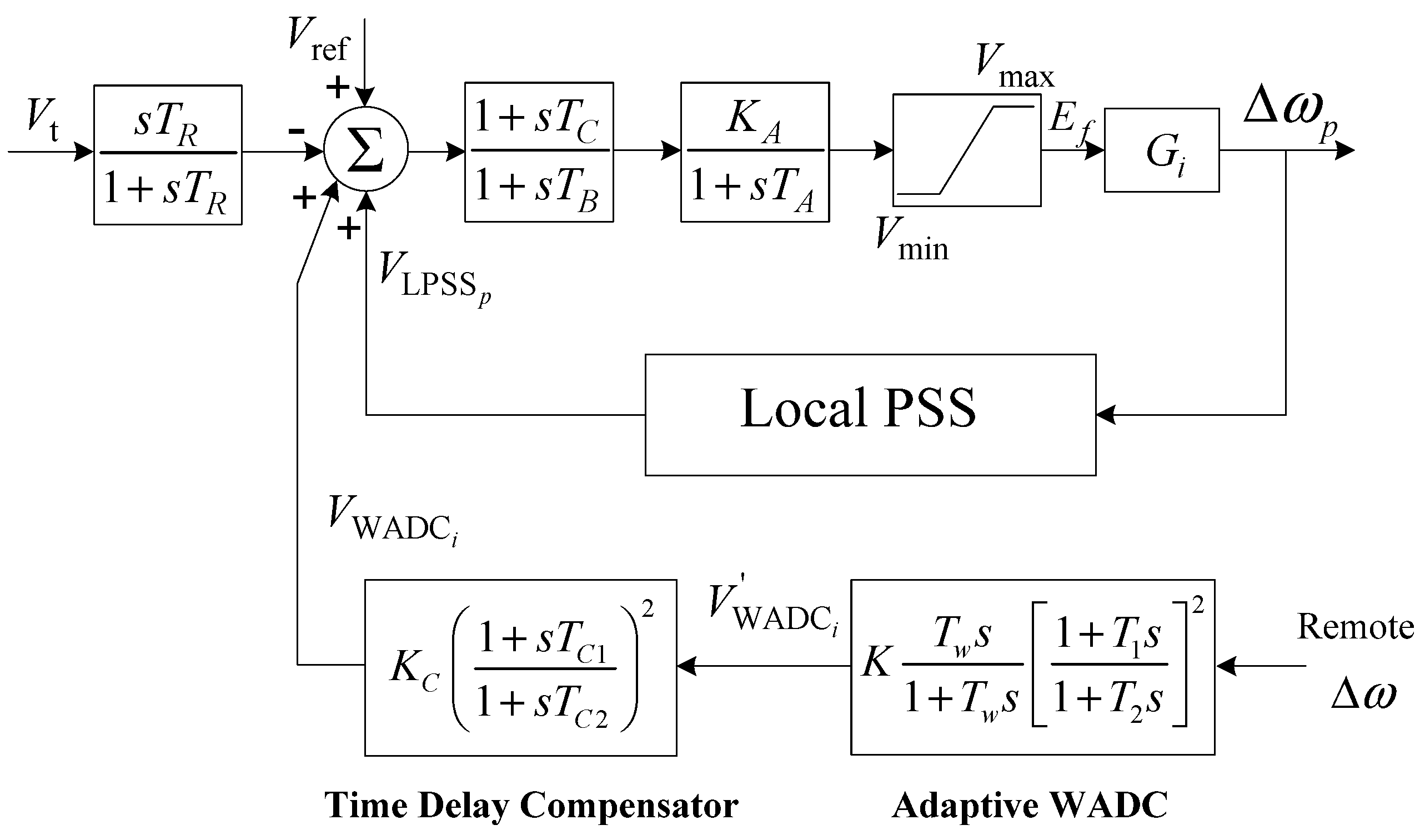
The exciter model with a two-layer PSS structure is shown in
Figure 1. The two-layer PSS structure serves the following two functions [
15]: (1) both local and inter-area oscillation modes can be suppressed; and (2) in case the adaptive WADC fails to act due to loss of PMU data or communication network failure, the independent local power system stabilizer (LPSS) remains operational and is capable of suppressing local oscillation modes and supply a certain amount of damping to the inter-area oscillation modes.
Figure 1.
Exciter model with two-layer PSS structure.
Figure 1.
Exciter model with two-layer PSS structure.
2.1. Design of Adaptive WADC
Consider the linearized state-space model of a power system expressed form as:
Based on the results of eigenvalue analysis obtained from the state-space model as Equation (1), the WADC can be designed using the residue method [
16] in which the parameters of WADC are determined from the relationship between residue and system eigenvalues.
Once the left eigenvectors
ei and right eigenvectors
fi are available, the residue of oscillation mode
i can be written as:
and the system transfer function can be described as:
where
is the continuous time system eigenvalue.
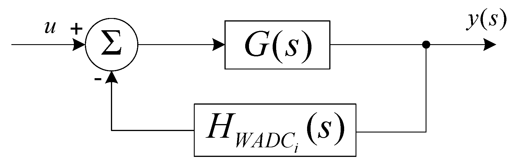
Now consider that
WADCi is added to improve the damping of oscillation mode
i as shown in
Figure 2. The eigenvalues of the new system are the roots of the following characteristic function:
If the change introduced to
is small, the change in
can be approximated as:
Figure 2.
Insertion of a PSS with a small gain in the system.
Figure 2.
Insertion of a PSS with a small gain in the system.
Since the objective of the
WADCi is to improve the damping of oscillation mode
i without changing its oscillation frequency,
shall be a negative real number so as to shift
horizontally to the left on the complex plane,
i.e.,:
where
φi is the compensation angle needed for oscillation mode
i. Here, the following classic transfer function with two stages of lead-lag blocks is adapted for
WADCi:
where
Ki determines the damping of oscillation mode
i;
is the wash-out time constant with a typical value of 5–10 s;
T1 and
T2 are the lead and lag time constants, respectively. Once the desired damping is fixed, the required displacement of
,
i.e.,
, could be determined; and the
WADCi parameters can then be calculated as follows [
17]:
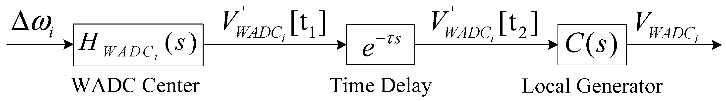
2.2. Signal Time Delay Compensator
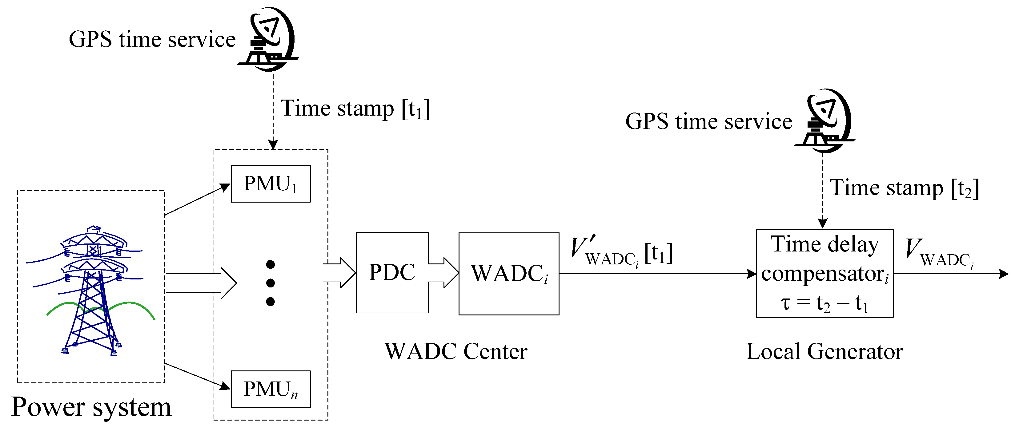
The signal time delay, mainly introduced by the long distance transmission of control signals from the WADC to the target generator, is significant and shall be compensated locally and is further illustrated in
Figure 3 with details.
Figure 3.
Scheme of time delay compensation.
Figure 3.
Scheme of time delay compensation.
Accurate time from the GPS would be received locally in both PMUs and the time delay compensator. Wide-area phasors measured by the PMUs at time t1 are collected and resynchronized by the phasor data concentrator (PDC) and in turn processed by the adaptive WADC to generate the wide-area damping control signal with time stamp [t1]. When the local time delay compensator, which is installed close to the generator exciter, receives the control signal [t1], the signal will be re-labeled with a new time stamp [t2] freshly obtained from the GPS and the exact time delay can be calculated accurately as because of the high resolution time service provided by the GPS.
In the presented study, the signal time delay is expressed by an exponential function
where
gives the signal delay time. Once the time delay is derived from the time stamps, it can be modeled and compensated as shown in
Figure 4.
Figure 4.
Time delay modeling and compensation.
Figure 4.
Time delay modeling and compensation.
With the time delay taking into consideration, the displacement in
would become:
where
and
. This means that the signal time delay effects on the displacement of
can be decomposed into gain drift
and phase lag
. If
is passed to the local generator along with the wide-area control signal
[
t1], the time delay could be compensated locally using the following transfer function with parameters tuned using the same approach for WADC parameter tuning outlined in [
18].
2.3. Synthesis of Wide-Area Control Signals
For each oscillation mode
i, there is a corresponding cluster pair, say
A1 and
A2. Since power oscillation between the clusters would have a nearly fixed phase relationship with the angular speed difference
between the clusters,
is selected and synthesized as a robust and effective wide-area control signal [
18] feeding to the most participated generator determined by the participation factors:
where
Hj is the inertia constant of generator
j and the control signal
for inter-area oscillation mode
i is determined by the angular speed difference between the areas oscillating with each other.
3. Subspace Identification Technique Based State-Space Model Estimation
In order to design the adaptive WADC, the linearized state space model and the interested information of the critical inter-area oscillation modes should be derived from the measurement. The subspace identification technique (SIT) is widely used in building numerically reliable state-space models for complex dynamic system from the measured data because of its numerical simplicity and robustness. In this paper, the subspace system identification technique (SIT) [
19] is adopted to derive state-space models online using measured signals to tune the parameters the WADC for suppressing inter-area oscillations.
3.1. State-Space Model Estimation
The linear time-invariant system, operating in discrete time, can be expressed in the state-space form [
19]:
where the vectors
and
are the measurements at time instant
k respectively; the vector
x(
k) is the state vector of the process at discrete time instant
k;
Ad,
B,
C, and
D are matrices with appropriate dimensions.
For system identification, given a set of measurements of the input u(k) and the output y(k), determine the order Norder of the unknown system, the system matrices (Ad, B, C and D).
Because of non-iterative, the numerical dynamic algorithm for subspace state-space system identification (N4SID) method has been used to derive the state-space model from the dynamic responses in this study. N4SID algorithms are performed as the following [
20]:
3.2. Modal Analysis and Mode Shape Identification
It shall be noted that
Ad obtained in Equation (18) is the discrete time state matrix. The discrete time state matrix
Ad can be expressed as follows:
where
is the eigenvalue of the discrete time system for
and
is the eigenvector matrix of the discrete time system. The continuous time system eigenvalue
can be calculated from the discrete system eigenvalue
as follows [
21]:
and the oscillation mode parameters can then be calculated as:
where
is the oscillation frequency and
is the damping ratio. Finally, the oscillation mode shape matrix
can be calculated as the mode observability matrix as follows [
21]:
3.3. Identification of Generators Needed to Be Supplemented by WADC
Based on the modal analysis theory, participation factor is defined as [
1]:
where
ajj is a diagonal element of the system matrix.
The system modes and its parameters can be obtained by digging the matrix Ad. However, it may be very difficult to calculate the participation facts of modes in the states since the state vector of the identified model is not corresponding to that of the real system which can be derived from the system structure and parameter by analytical methods.
To appropriately handle this problem, the similarity transformation is applied. Using
T =
dia(
λ1,
λ2, …,
λN) as a similarity transformation matrix, the following modal canonical realization can be obtained [
22]:
where
,
,
.
Considering the output of Equation (24), the following equation can be formulated:
Therefore, the output
yj is affected by mode
λk and mode in output the measurement based participation factor is proposed as:
In order to determine the contribution factors,
z0 is needed and it can be provided using the following relation:
Moreover, the right eigenvectors determined by using Equation (22) are selected as the initial condition [
22],
x0.
As we see in the published papers, the participation factors are generally indicative of the relative participations of the respective states in the corresponding modes [
1]. The participation factors can be used to select the installation locations of LPSS. In this paper, the measurement-based participation factors are used to select the generators that need to be supplemented by WADC. For the critical inter-area oscillation mode, the generators in each oscillation group are ordered according to the measurement based participation factors, and then the first two generators are identified to supplement the WADC.
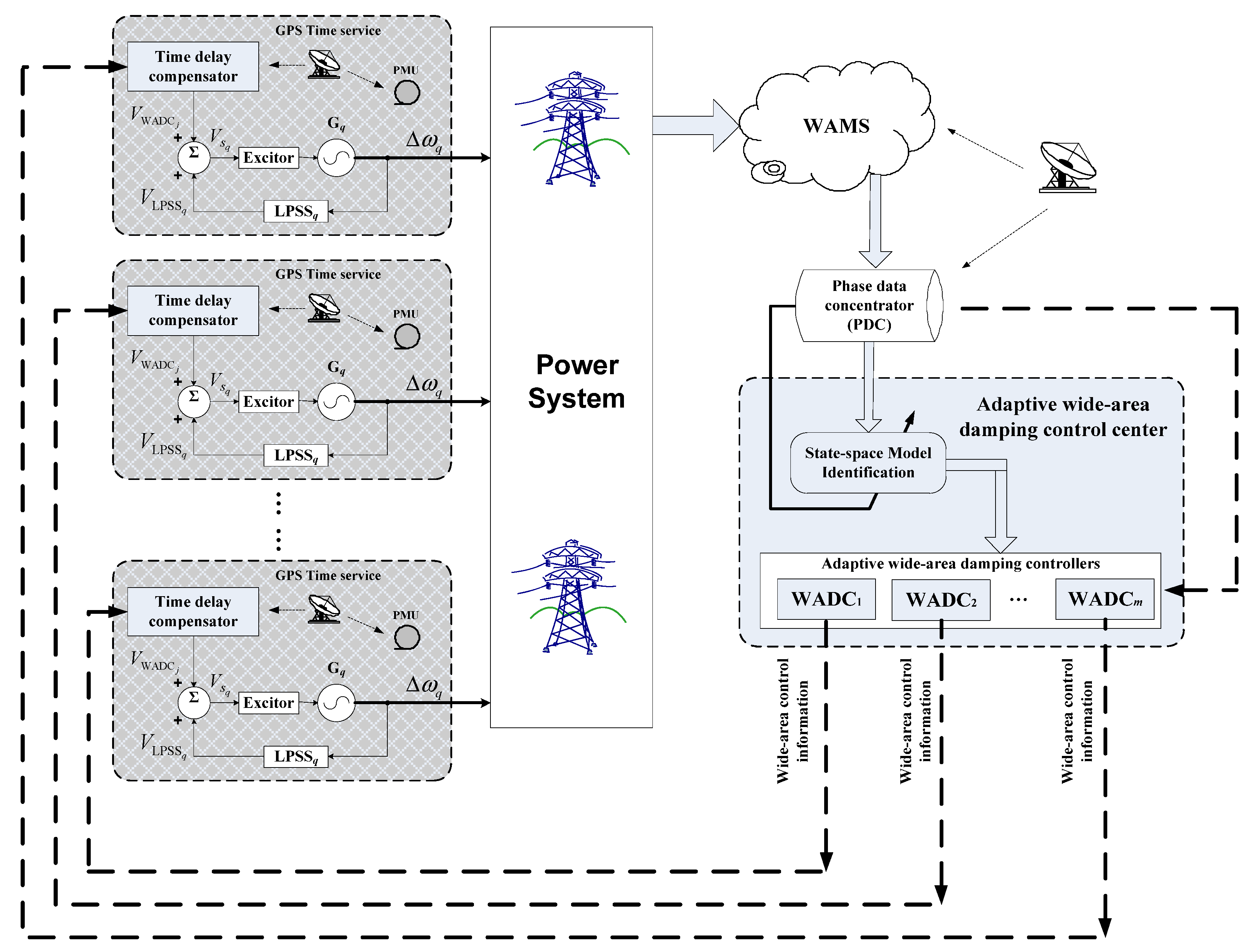
4. Adaptive Wide-Area Damping Control Scheme and Control Flow
The proposed adaptive wide-area damping control scheme with online state-space model identification and consideration of time delay is shown in
Figure 5.
Figure 5.
Adaptive wide-area damping control scheme with consideration of signal time delay.
Figure 5.
Adaptive wide-area damping control scheme with consideration of signal time delay.
Via the PMU data collection system, the speed signals of all PMU-equipped generators are measured and transmitted to the wide-area damping control center. In case a power oscillation arises, local oscillation modes could be suppressed by the LPSS in each generator while the adaptive WADC would be used to suppress the detected inter-area oscillations. The suppression mechanism adopted here is that: (1) state-space model, low-frequency inter-area oscillation modes, and the corresponding generator oscillation groups will first be identified online based on the SIT; (2) for the critical mode with insufficient damping, the parameters and input of the corresponding WADC will be tuned and derived to suppress the power oscillation; and (3) the output of each WADC will be sent to generators and be compensated locally for the transmission time delay.
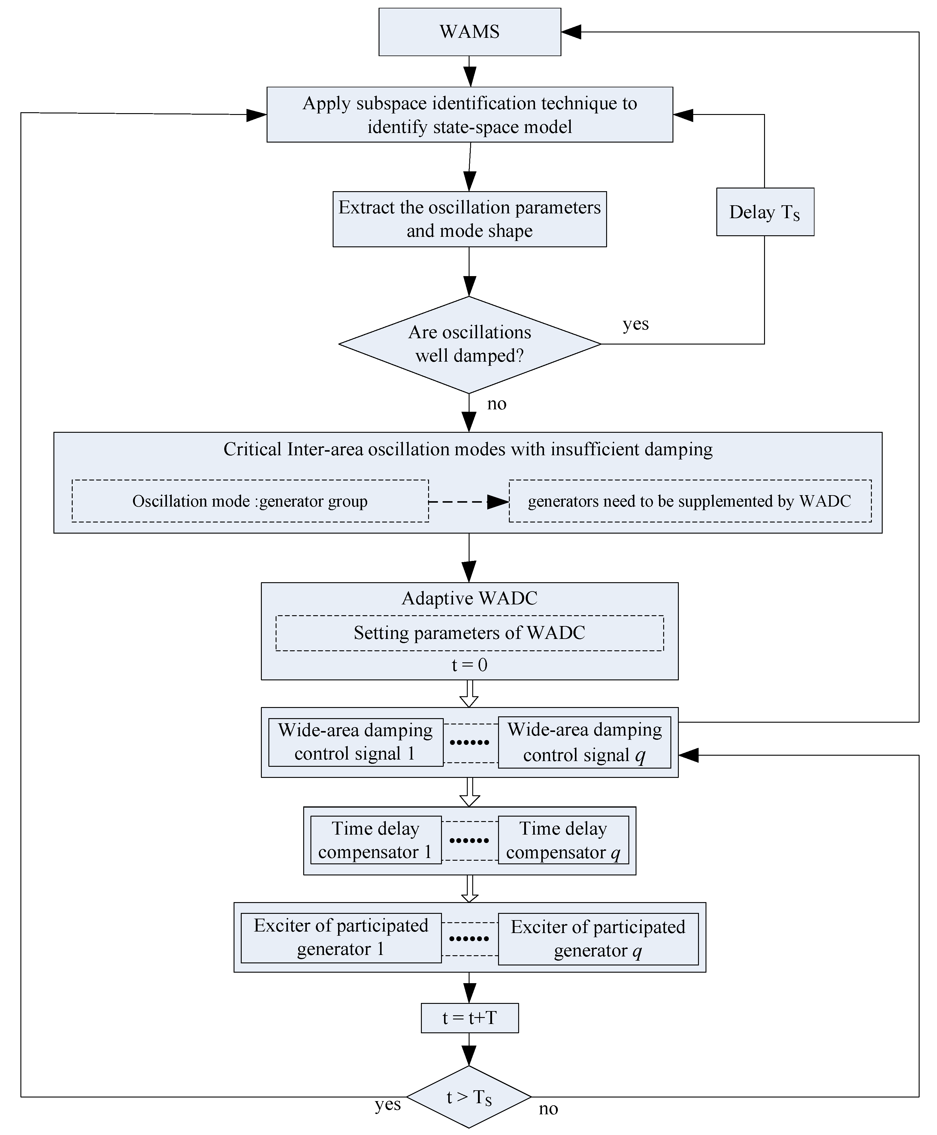
Figure 6 shows the overall flow chart of the proposed adaptive wide-area damping control scheme which mainly consists of the subspace identification algorithm based state-space model estimation, oscillation parameter extraction, adaptive WADC and time delay compensator described in previous sections. The control algorithm operates on windows of WAMS data with cycle time
TS and could be triggered by timer, events or operator.
Figure 6.
Flow chart of the proposed adaptive wide-area damping control scheme.
Figure 6.
Flow chart of the proposed adaptive wide-area damping control scheme.
The following are the major steps involved in a cycle:
- Step 1:
Apply the subspace system identification technique on a window of WAMS data collected in the last cycle to identify the state-space model of the system.
- Step 2:
Extract the inter-area oscillation modes.
- Step 3:
If there is any inter-area oscillations with damping below, say, 5% [
23], proceed to the following step to activate the adaptive wide-area damping control; otherwise, wait till the next cycle while collecting WAMS data and return to Step 1.
- Step 4:
Determine the critical inter-area oscillation modes with the smallest damping ratio and the corresponding oscillation generator group and the generators with lager participation factor in each oscillation group for the critical inter-area oscillation mode.
- Step 5:
Construct adaptive WADCs for the generators need to be supplemented by WADC with parameters calculated using Equation (8), and set t = 0.
- Step 6:
Measure the signal time delay locally in the generator with the help of high resolution GPS time service and apply the signal time delay compensation to produce the required wide-area control signal feeding to the generator exciter in order to increase damping of the targeted inter-area oscillation mode.
- Step 7:
Increment t by one time-step TS and go back to Step 5 to continue the control action until next cycle.
- Step 8:
Go back to Step 1 to start a new cycle of adaptive wide-area control.
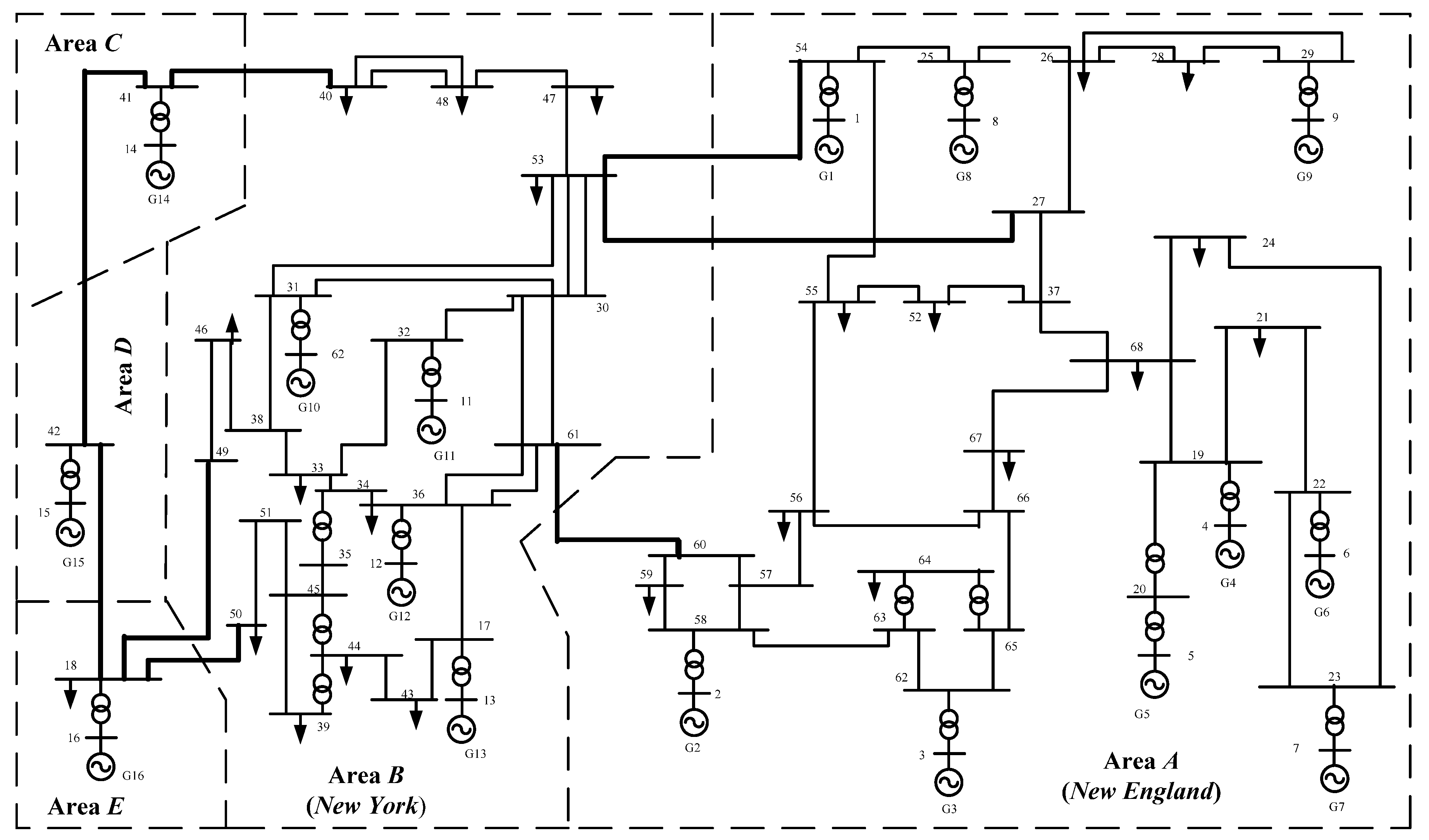
5. Simulation Studies
The IEEE 16-generator 5-area test system shown in
Figure 7 was selected as the benchmark system for evaluating the performance of the proposed adaptive wide-area damping control scheme with consideration of signal time delay.
Figure 7.
IEEE 16-generator 5-area test system.
Figure 7.
IEEE 16-generator 5-area test system.
System data for this system is available in [
24]. This system can be divided into five areas, namely, A—New England (G1–G9); B—New York (G10–G13); C—Equivalent Generator G14; D—Equivalent Generator G15; and E—Equivalent Generator G16. LPSSs are equipped in G1–G16. The cycle time and time step adopted for the adaptive WAMS based wide-area control and the time domain simulation are 3 s and 20 ms, respectively. In order to fully test the effectiveness of the proposed adaptive wide-area damping control scheme, the following two operation scenarios are considered:
- (A)
Operation scenario a:
In this operation scenario, approximately 800 MW power flows from Area A to Area B over the tie line (line 27–53, line 53–54 and line 60–61). The inter-area mode, (G1–G9) vs (G10–G13), is the critical mode and is excited by the following disturbances:
Case a1: a 3-phase solid self-clearing fault at bus 27 for 50 ms.
Case a2: a 3-phase solid fault occurs in the beginning of the line between bus 30 and 32 at time t = 1.0 s, and is cleared with the faulty line tripped after 100 ms.
- (B)
Operation scenario b:
In this operation scenario, only approximately 200 MW power flow from Area A to Area B over the tie line (line 27–53, line 53–54 and line 60–61). The inter-area modes, (G1–G13) vs. (G14–G16) and G15 vs. (G14 and G16), are the critical mode and are excited by the following two disturbances, respectively:
Case b1: a 3-phase solid self-clearing fault at bus 49 for 50 ms.
Case b2: line 18–49 was tripped at 1.0 s because of fault.
5.2. Effectiveness of the Adaptive Wide-Area Damping Control Scheme
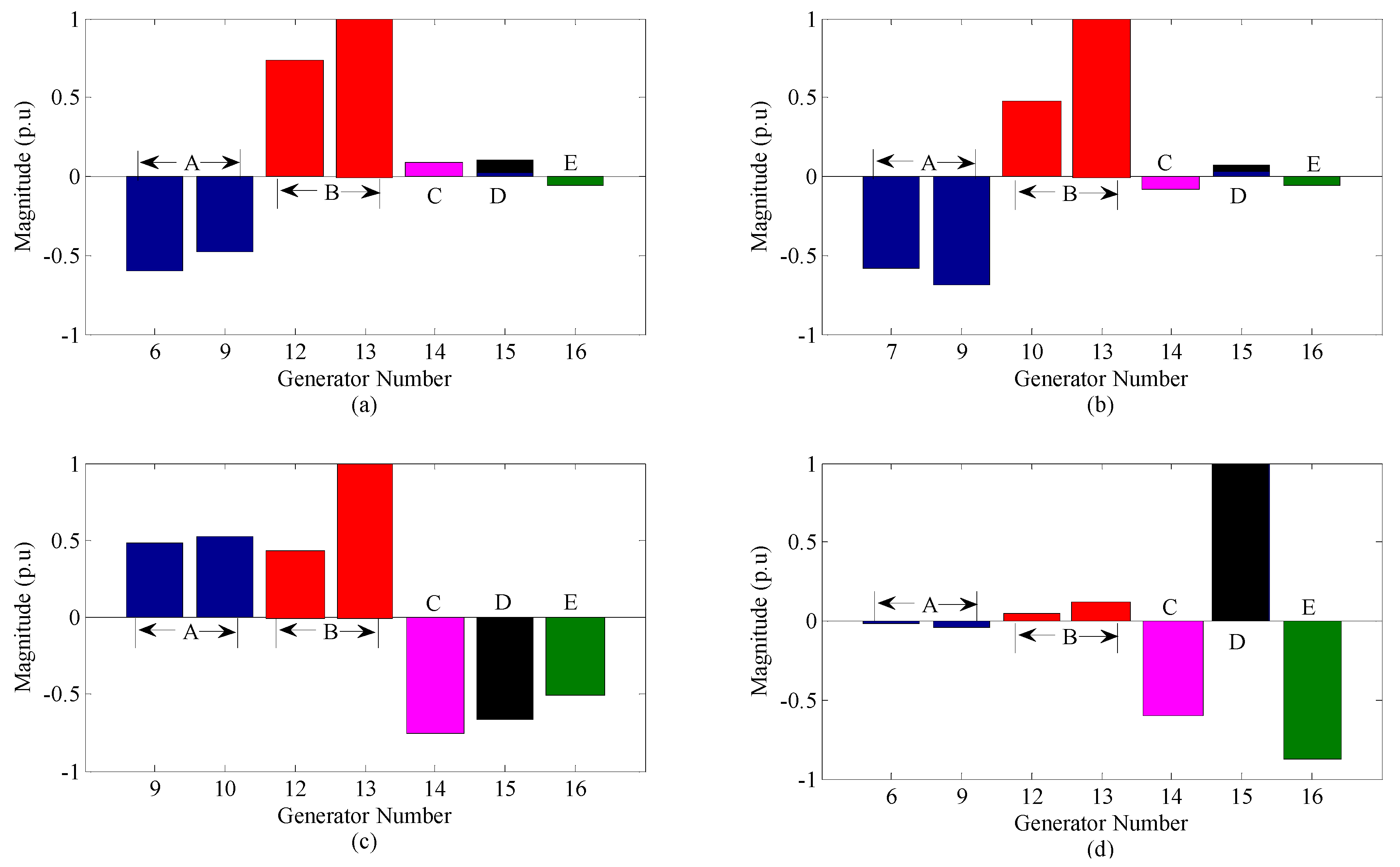
As shown in
Table 1, four critical inter-area oscillation modes with insufficient damping in each disturbance scenario were identified and detected. The corresponding oscillation generator clusters and the generators need to be supplemented by WADC in each oscillation group were then identified, as shown in
Figure 8. To suppress the critical inter-area oscillation modes with insufficient damping in each disturbance scenario, four WADCs were constructed accordingly with input derived from the live WAMS data, output fed to the exciter of the generators with lager participation factor, and details listed in
Table 3.
Table 3.
Results of control signal and generators that need to be supplemented by WADC.
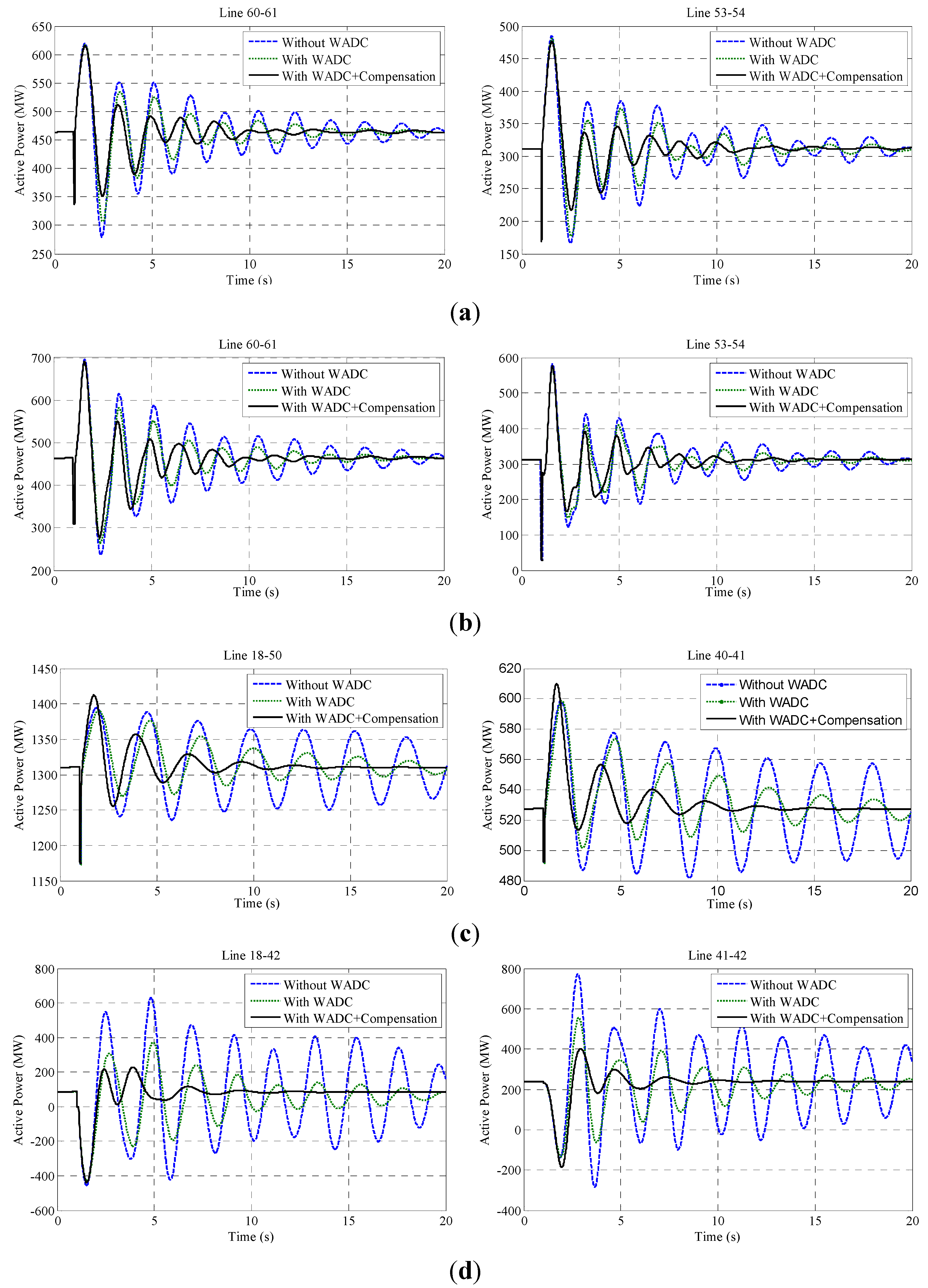
A comparison study on the effectiveness of inter-area oscillation control in the four disturbance scenarios with no WADC (only LPSS), WADC only, and WADC plus the time delay compensation under different time delay conditions was conducted, with results shown in
Figure 8, which plots the selected line flow for the four above-mentioned cases with no WADC, WADC only, and WADC plus the time delay compensation under different time delay conditions. Because of insufficient damping in the critical inter-area oscillation modes, the system will take quite a long time to settle down if only LPSSs are installed. However, with the help of the proposed adaptive WADCs, oscillations are quickly suppressed in all cases as shown in
Figure 9.
Because of the wide spread of the inter-connected power system, signal transmission delays cannot be ignored. Typically, the signal time delay in WAMS is on the order of 100 ms, but could be longer if the communication links are busy and congested. In this study, signal time delays in the range from 50 to 250 ms were added randomly.
Figure 9.
Plots of the active power of the selected tie-line for case a1–b2. (a) Active power for case a1 with consideration of 200 ms time delay; (b) active power for case a2 with consideration of 150 ms time delay; (c) active power for case b1 with consideration of 100 ms time delay; and (d) active power for case b2 with consideration of 80 ms time delay.
As shown in
Figure 9, it is clear when the signal time delay was included but not compensated, the effectiveness of the wide-area control was severely deteriorated, whereas the responses when including signal time delay and compensation took a short time to settle down. This shows that the proposed signal time delay compensation works well and provides better damping to the inter-area oscillation.
The investigations on the different four disturbance scenarios demonstrate that the effectiveness of the WADCs is significantly deteriorated without the time delay compensation and the proposed time delay compensation scheme works very well.
6. Conclusions
This paper proposes a novel adaptive wide-area control scheme with consideration of signal time delay. The proposed control scheme is mainly composed of three parts: SIT algorithm based state-space model estimation, adaptive WADC and signal time delay compensator. When an oscillation is detected in a power system, first the SIT algorithm would be used to effectively and robustly estimate the state-space model and identify the inter-area oscillation mode on-line. According to the critical inter-area oscillation modes with insufficient damping, a self-adaptive WADC would then be constructed with parameters tuned to increase the damping torque of the targeted oscillation modes by transmitting the control signals to the generators via the WAMS. The effects of signal time delay on the damping control are effectively eliminated using a local signal time delay compensator installed close to the target generators.
Through the case studies conducted on the IEEE 16-generators 5-area test system, the effectiveness of the proposed wide-area damping control scheme is proven. When signal time delay is considered in the simulation, the proposed signal time delay compensator can effectively eliminate the effects of the delay on the performance of the adaptive WADC.


