Short-Term Wind Power Forecasting Using the Enhanced Particle Swarm Optimization Based Hybrid Method

Abstract

High penetration of wind power in the electricity system provides many challenges to power system operators, mainly due to the unpredictability and variability of wind power generation. Although wind energy may not be dispatched, an accurate forecasting method of wind speed and power generation can help power system operators reduce the risk of an unreliable electricity supply. This paper proposes an enhanced particle swarm optimization (EPSO) based hybrid forecasting method for short-term wind power forecasting. The hybrid forecasting method combines the persistence method, the back propagation neural network, and the radial basis function (RBF) neural network. The EPSO algorithm is employed to optimize the weight coefficients in the hybrid forecasting method. To demonstrate the effectiveness of the proposed method, the method is tested on the practical information of wind power generation of a wind energy conversion system (WECS) installed on the Taichung coast of Taiwan. Comparisons of forecasting performance are made with the individual forecasting methods. Good agreements between the realistic values and forecasting values are obtained; the test results show the proposed forecasting method is accurate and reliable.

1. Introduction

The gradual shortage of oil and worldwide awareness of environmental issues highlights the exploitation of renewable energy technologies. Wind power is one of the most attractive renewable energy applications because of its high efficiency and low pollution [1]. In fact, wind power is the fastest growing source of renewable energy. In mid-2012, the capacity of the wind energy conversion system (WECS) reached 254 GW, with 273 GW expected for a full year. Global wind capacity has grown by 7% in the past six months and by 16.4% annually [2]. Large-scale wind penetration requires answers to a lot of problems such as low voltage ride through [3], spinning reserve capacity scheduling, utility grid control and operation, and ancillary service scheduling. An accurate wind forecasting method is known as an efficient tool to overcome these problems [4,5].

To reduce the spin reserve margin capacity and increase wind power penetration, accurate forecasting of wind power is needed for power system operations [6]. Accurate wind power forecasting can help improve the stability of the utility grid, reliability of the power system, and the quality of power [7]. In addition, wind power forecasting is important in the allocation of balancing power. Wind power forecasting is used for the day-ahead scheduling of conventional power plants and the trading of electricity on the competitive market [8]. Although the prediction accuracy of wind power forecasting is lower than that of load forecasting. Wind power forecasts still play a key role in addressing the operation challenges of a utility grid [9].

Recently, several methods are employed for wind power forecasting. Many studies have been devoted to improvements in wind power forecasting approaches by researchers with wide experience in the field tests. A number of wind power forecasting methods have been developed and launched on wind farms. The wind power forecasting methods can be generally categorized into six groups [1]: persistence method, physical method, statistical method, spatial correlation method, artificial intelligence (AI) method, and hybrid method.

The persistence method is not only the simplest, but is also the most economical wind speed or power forecasting method. Electrical utility uses the persistence method for ultra-short-term forecasts. Any forecast method that is developed should first be tested against the classical benchmark of the persistence method to check how much it can improve over the persistence derived forecasts [7].

Physical methods use parameterizations based on a detailed physical description of the atmosphere, to reach the best prediction precision. Usually, the wind speed given by the weather service on a coarse grid is transformed to the onsite conditions at the location of the wind farm [8]. Existing commercial wind power forecasting methods use numerical weather prediction (NWP) wind forecasts as the input data. Physical systems, using the input data from NWP, carry out the necessary refinement of these output data (wind speed forecast) to the on-site conditions by methods that are based on the physics of the lower atmospheric boundary layer [10].

Statistical methods include the auto regressive (AR), auto regressive moving average (ARMA), auto regressive integrated moving average (ARIMA), Bayesian approach, and gray predictions. Statistical methods can be used to solve the problems in forecasting having a great deal of data where the observations are interdependent. Basically, the statistical method is good for short-term prediction. The disadvantage with this method is the prediction error increases as the prediction time increases [9].

The spatial correlation methods take the spatial relationship of different sites’ wind speed into account. In spatial correlation models, the wind speed time-series of the predicted point and its neighboring points are employed to predict wind speed [6]. Based on spatial correlation models, the technique for forecasting wind speed and power output up to several hours ahead, using the cross correlation at neighboring sites. The paper developed an artificial neural network (ANN) approach that significantly improves forecasting accuracy compared to the persistence forecasting method [11]. The spatial correlation method is used for predicting wind speed at one site based on measurements at another site [12].

Recently, with the development of AI, various new AI methods for wind speed and power prediction have been developed. AI methods mimic the learning processes of the brain to discover the relations between the variables of a system [9]. The new developed AI methods include the ANN, adaptive neuro-fuzzy inference system, fuzzy logic methods, support vector machine, neuro-fuzzy network, and evolutionary optimization algorithms.

ANN can deal with non-linear and complex problems in terms of classification or forecasting. The ANN models can represent a complex nonlinear relationship and extract the dependence between variables through the training process [13]. ANN based methods include back propagation neural networks, radial basis function (RBF) neural networks, recurrent neural networks, the ridgelet neural network, and the adaptive linear element neural network. The ANN based method is an appropriate method to apply to the problem of forecasting wind power.

The object of hybrid wind forecasting methods is to benefit from the advantages of an individual model and obtain a globally optimal forecasting performance. In reference [14], a hybrid forecasting method combines evolutionary particle swarm optimization with an adaptive-network-based fuzzy inference system (ANFIS) is proposed. In this method, the evolutionary particle swarm optimization is used to improve the performance of ANFIS, tuning the membership functions required to achieve a lower error. Since the information contained in the individual forecasting method is limited, the hybrid method can maximize the available information, integrate individual model information, and make best use of the advantages of multiple forecasting methods, thus improving forecasting accuracy [10]. The literature shows the hybrid methods generally produce good wind forecasting results compared to individual models [9]. The hybrid methods combine different approaches such as mixing physical and statistical approaches or combining short-term and medium-term models [7].

To increase the accuracy of short-term wind power forecasting this paper takes the hybrid method and presents a combined forecasting model to account for the nonlinearity and periodicity in the wind power generation time series. The following forecasting methods are combined for the hybrid method: the persistence method, the back propagation neural network method, and the RBF neural network method.

This paper deals with the power generation forecasting of WECS and is divided into six sections. After a brief introduction, Section 2 introduces the individual forecasting methods used in the hybrid method. Section 3 describes the combination theory of the hybrid method. Section 4 describes the determination of the weight coefficients of the hybrid method by enhanced particle swarm optimization (EPSO) algorithm. Numerical results are described in Section 5. The conclusions of the paper are summarized in Section 6.

2. Individual Forecasting Methods Used in the Hybrid Method

2.1. Persistence Method

The persistence method is based on a simple assumption that the wind speed and wind power at a certain future time will be the same as it is when the forecast is made [15]. If the measured wind speed and wind power at t are v(t) and P(t), then the forecasting wind speed and wind power at t + Δt can be formulated as the following term:

v(t + Δt) = v(t)

(1)

P_o(t + Δt) = P_o(t)

(2)

The persistence method is somehow more accurate than other wind forecasting methods in ultra-short-term forecasting. However, the accuracy of the persistence method will degrade rapidly when the time-scale of forecasting is increasing [14].

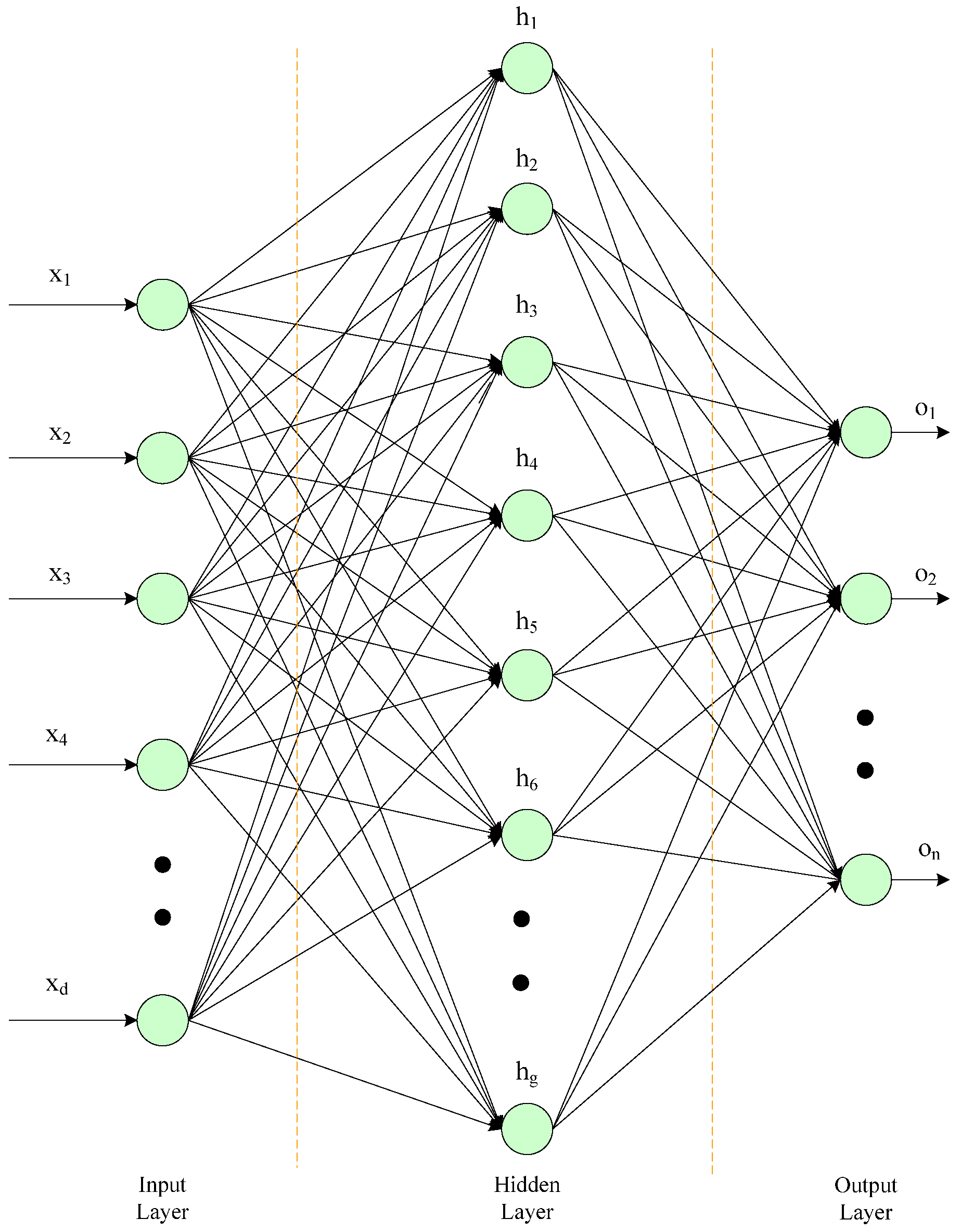
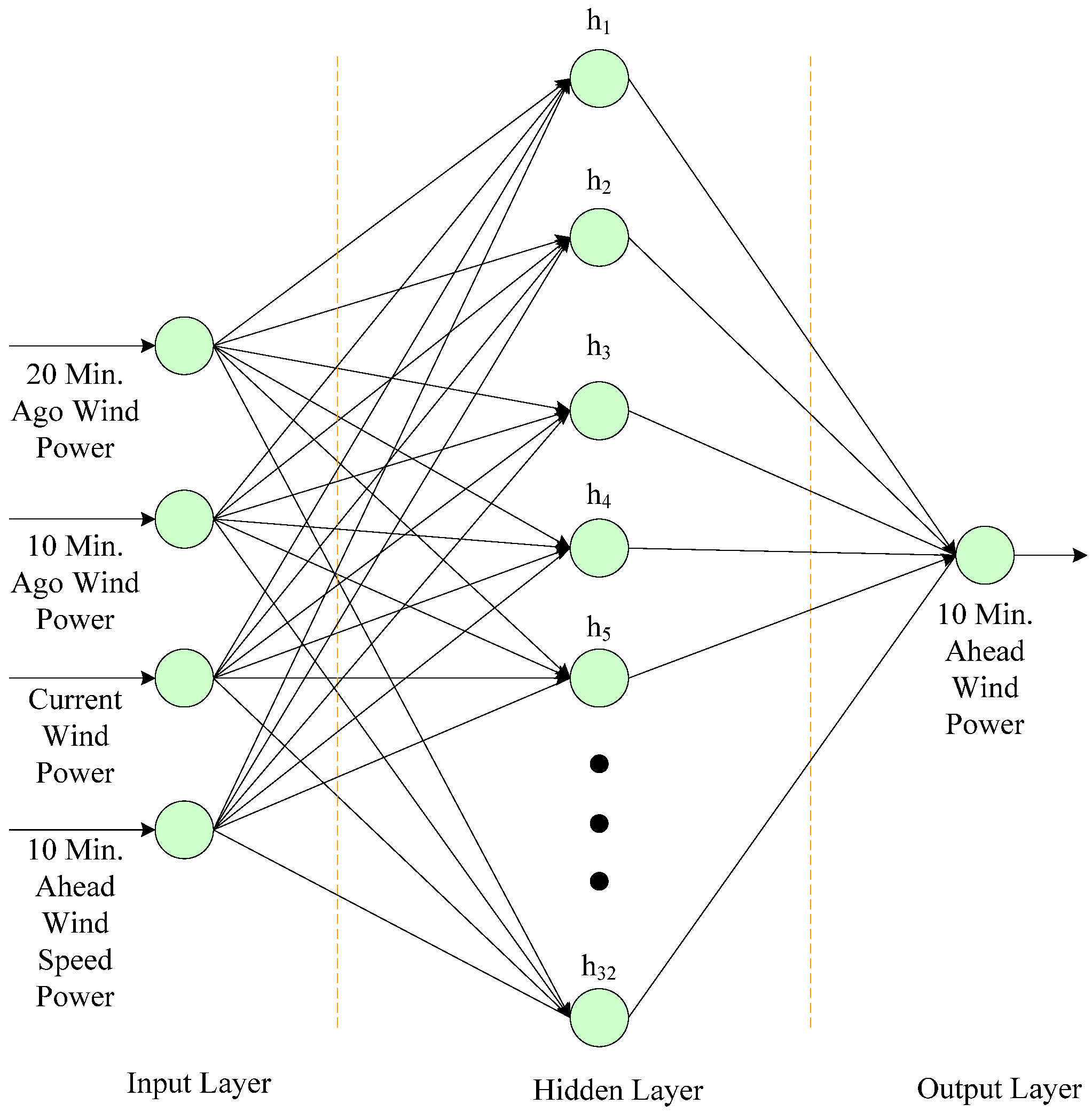
2.2. Back Propagation Neural Network Method

The back propagation neural network is a multi-input, multi-output system consisting of an input layer, one or two hidden layers, and an output layer. Each layer employs several neurons, and each neuron in a layer is connected to the neurons in the adjacent layer with different weights. The architecture of a typical back propagation neural network is shown in Figure 1. The network actually performs a nonlinear mapping from the input space R^d to the output space Rⁿ. The mapping relationship between the input vector and output vector of a back propagation neural network is based on the following function:

$$\begin{array}{cccc}Back& propogation& neural& network:\end{array}\{\begin{array}{c}{R}^d\to R^n\\ \overrightarrow{x}\to \overrightarrow{o}\end{array}$$

(3)

where input vector $\overrightarrow{x}$ = {x₁, x₂, ....., x_d}; and output vector $\overrightarrow{o}$ = {o₁, o₂, ....., o_n}.

Signals flow into the input layer, pass through the hidden layer, and arrive at the output layer. With the exception of the input layer, each neuron receives signals from the neurons of the previous layer. The incoming signals are multiplied by the weights and summed up with the bias contribution.

The total input of a neuron in hidden layer is calculated by the following form:

$$net{i}_j={\displaystyle \sum _{i=1}^d{x}_i{w}_{ij}+b_j}$$

(4)

where neti_j is the total input of the hidden layer neuron j; x_i is the input to the hidden layer neuron j from input layer neuron i; w_ij is the weight between the input layer neuron i and hidden layer neuron j; b_j is bias of the hidden layer neuron j; and d is the number of neurons in the input layer.

The activation function applied to the neuron in the hidden layer is the hyperbolic tangent function which is calculated by the following equation:

$$h_j=f(net{i}_j)=\frac{1-e^{-2net{i}_j}}{1+e^{-2net{i}_j}}$$

(5)

Figure 1. Architecture of the back propagation neural network and radial basis function (RBF) neural network.

Figure 1. Architecture of the back propagation neural network and radial basis function (RBF) neural network.

The total input of a neuron in output layer is calculated by Equation (6):

$$net{o}_j={\displaystyle \sum _{i=1}^g{h}_i{w}_{ij}+k_j}$$

(6)

where neto_j is the total input of the output layer neuron j; h_i is the input to the output layer neuron j from hidden layer neuron i; w_ij is the weight between the hidden layer neuron i and output layer neuron j; k_j is the bias of the output layer neuron j; and g is the number of neurons in the hidden layer.

The activation function applied to the neuron in the output layer is the sigmoid function, which is calculated by the following equation:

$$o_j=f(net{o}_j)=\frac{1}{1+e^{-net{o}_j}}$$

(7)

The procedure of estimating the weights between the layers and bias of the neurons can be calculated using the steepest descent algorithm. In training the network with a given architecture, the error back propagation approach finds a single best set weight and bias values by minimizing the suitable error function.

The back propagation neural network based wind power forecasting method has been successfully implemented using personal computer (PC)-based software for the wind power prediction [16]. The architecture of the wind power forecasting neural network is shown in Figure 2. The back propagation neural network models were developed for 10 min. ahead wind power forecasting. The architecture of the back propagation neural network-based wind power forecasting method is shown in Figure 2. The input layer has four neurons for the wind power output of 20 min ago, 10 min ago, the current wind power output, and 10 min ahead wind speed forecasting value; the hidden layer has 32 neurons and the output layer has one neuron for the 10 min ahead wind power forecasting.

The back propagation neural network based forecasting method is described briefly in the following steps:

Step 1

Create the database of the wind power generation of WECS;

Step 2

Normalize all of the wind power generation data;

Step 3

Prepare the training set for the back propagation neural network;

Step 4

Use the error back propagation algorithm to train the back propagation neural network for wind power forecasting;

Step 5

Save the weights between the layers and bias of the neurons of the trained back propagation neural network, as the training procedure is finished;

Step 6

Use the trained back propagation neural network to forecast the wind power generation of WECS.

Figure 2. Architecture of the back propagation neural network based and RBF neural network based wind power forecasting method.

Figure 2. Architecture of the back propagation neural network based and RBF neural network based wind power forecasting method.

2.3. RBF Neural Network Method

The architecture of a typical RBF neural network is shown in Figure 1. The network actually performs nonlinear mapping from the input space R^d to the output space Rⁿ [1]. The mapping relationship between the input vector and output vector of the RBF neural network is based on the following function:

$$\begin{array}{ccc}RBF& neural& network:\end{array}\{\begin{array}{c}{R}^d\to R^n\\ \overrightarrow{x}\to \overrightarrow{o}\end{array}$$

(8)

where input vector $\overrightarrow{x}$ = {x₁, x₂, ....., x_d}; and output vector $\overrightarrow{o}$ = {o₁, o₂, ....., o_n}.

Each hidden neuron computes a Gaussian function in the following equation:

$$h_j(\overline{x})=\exp [\frac{-{({\overline{x}}^T-{\overline{\mu }}_j)}^2}{2{\sigma }_j^2}],\begin{array}{cc}for& j=1,2,\mathrm{.......},g\end{array}$$

(9)

where μ_j and σ_i are the center and the width of the Gaussian potential function of the i-th neuron in the hidden layer, respectively.

Each output neuron of RBF neural network computes a linear function in the following form:

$$o_k={\displaystyle \sum _{j=1}^g{w}_{kj}{h}_j(\overline{x})+{\theta }_k,\begin{array}{cc}for& k=1,2,\mathrm{.......},n\end{array}}$$

(10)

where o_k is the output of the k-th node in the output layer; w_kj is the weight between the j-th node in the hidden layer and the k-th node in the output layer; $h_j(\overline{x})$ is the output from the j-th node in the hidden layer; and θ_k is the bias of the k-th node in the output layer.

The RBF neural network based wind power forecasting method has been successfully implemented for wind power forecasting. The RBF neural network models were developed for 10 min ahead wind power forecasting. The architecture of the RBF neural network-based wind power forecasting method is shown in Figure 2. The input layer has four neurons for the wind power output of 20 min ago, 10 min ago, the current wind power output and 10 min ahead wind speed forecasting value; the hidden layer has 32 neurons and the output layer has one neuron for the 10 min ahead wind power forecasting.

The RBF neural network based forecasting method is briefly described in the following steps:

Step 1

Create a database of wind power generation of WECS;

Step 2

Normalize all the wind power generation data;

Step 3

Prepare the training set for the RBF neural network;

Step 4

Using the training set to train the RBF neural network for wind power forecasting;

Step 5

Save the Gaussian functions centers, widths and connection weights between the hidden and output layers of the trained RBF neural network, as the training procedure is finished;

Step 6

Use the trained RBF neural network to forecast the wind power generation of the WECS.

3. The Combination Theory of the Proposed Hybrid Method

The input data of hybrid forecasting method are the wind power output of 20 min ago, 10 min ago, the current wind power output, and 10 min ahead wind speed forecasting value. The forecast data is the 10 min ahead wind power forecasting value. The combination theory of the hybrid method is based on if there are M kinds of forecasting methods for solving a certain forecasting problem, with properly selected weight coefficients, these forecasting methods’ results can be added up [17]. The mathematical model of the hybrid forecasting method is expressed in the following terms:

$$y_t={\displaystyle \sum _{i=1}^M{w}_i(y_{it}+e_{it})}$$

(11)

$${\widehat{y}}_t={\displaystyle \sum _{i=1}^M{\widehat{w}}_i{\widehat{y}}_{it}}$$

(12)

where y_t (t = 1, 2, …, L) is the actual time series data; L is the number of sample points; ${\widehat{y}}_{it}$ (i = 1, 2, …, M, t = 1, 2, …, L) is the forecasted value obtained by the i-th forecasting method, e_it = y_t − ${\widehat{y}}_{it}$ is the forecasting error; w_i is the weight coefficient for the i-th forecasting method; ${\widehat{w}}_i$ is the estimated value for w_i; and ${\widehat{y}}_t$ is the combined forecasting value of the hybrid method.

Determination of the weight coefficients for each individual method is the most important step in the construction of a hybrid forecasting method. The weight coefficients can be achieved by solving an optimization problem which minimizes the absolute error of the hybrid method. The mathematical model of optimization problem can be expressed in the following term:

$$Min{\displaystyle \sum _{t=1}^L\left|y_t-{\widehat{y}}_t\right|}\hspace{1em}\hspace{1em}\begin{array}{ccc}\begin{array}{cc}subject& to\end{array}& {\displaystyle \sum _{i=1}^M{w}_i=1}& 0\le w_i\le 1\end{array}$$

(13)

The optimization problem is solved by the EPSO algorithm in this paper. The optimization process can be terminated when the predefined absolute error has been received or the maximum iteration time has been reached [17].

4. Determining Weight Coefficients of Hybrid Method by EPSO Algorithm

4.1. Principle of EPSO Algorithm

A particle swarm optimization (PSO) algorithm is developed for solving continuous optimization problems and this is a population based stochastic technique [18]. The PSO algorithm is considered an effective tool for solving engineering optimization problems for ordinary differential equations [19]. Each individual in the PSO flies in the search space with a velocity which is dynamically adjusted according to its own flying experience and flying experience of its companions [20]. In a PSO system, each particle saves its own best position and also saves the best position found so far in the search-space by which all the swarm is expected to move toward it [21].

In a PSO algorithm, all particles are manipulated according to Equations (14) and (15). In the D-dimensional space, each particle has a position vector p_i = (p_i1, p_i2,…, p_iD) and a velocity vector v_i = (v_i1, v_i2,…, v_iD) (i = 1, 2,…, N), where N is the number of particles in the swarm. Each particle tries to adjust its velocity according to the best previous position stored in its memory, termed a personal best (denoted as pbest), and according to the best previous position attained by any particle in swarm, termed the global best (denoted as gbest), to search for a better position. The movement equations for the i-th particle are as follows:

$$v_{id}(t+1)=\omega \times v_{id}(t)+{\eta }_1\times r_1[pbest-p_{id}(t)]+{\eta }_2\times r_2[gbest-p_{id}(t)]$$

(14)

$$p_{id}(t+1)=p_{id}(t)+v_{id}(t+1)\hspace{1em}\hspace{1em}\begin{array}{cc}i=1,2,\mathrm{...},N& d=1,2,\mathrm{...},D\end{array}$$

(15)

where v_id(t) and v_id(t + 1) are the current and modified velocity for each iteration, respectively; and η₁ and η₂ are positive numbers, used to control the particle’s movement at each iteration. They represent cognitive and social components, respectively. r₁ and r₂ are uniformly distributed numbers in the range [0, 1], and p_id(t) and p_id(t + 1) are the current and modified position for each iteration, respectively. ω denotes the inertial weight, which is set according to the following equation [19]:

$$\omega ={\omega }_{\max }-\frac{{\omega }_{\max }-{\omega }_{\min }}{t_{\max }}\times t_n$$

(16)

where t_max is the maximum number of iterations; and t_n is the current number of iterations. Equation (16) restricts the value of ω to the range [ω_max, ω_min].

Equation (14) shows the search procedure of the PSO heavily depends on the values of pbest and gbest. If the initial population of particles cannot effectively cover the whole region, the particles usually converge on a local optimal solution and not a global optimal solution. To avoid these limitations, this paper incorporates a mutation mechanism for the evolutionary computation into the PSO algorithm, termed an EPSO algorithm [22]. In general, particles with poor individuals are selected for mutation from a subset of the swarm.

The next position of the i-th particle selected for mutation is modified by:

$$p_{id}(t+1)=p_{id}(t)+N(0,{\sigma }_i^2)\hspace{1em}\hspace{1em}\begin{array}{c}i=1,2,3,\mathrm{.....},Z\end{array}$$

(17)

where N(0, σ_i²) is a vector of the Gaussian random variables with a mean of zero and a standard deviation σ_i; and i = 1,2,….,Z, where Z is the number of particles selected for mutation. Generally, Z is set at 10% of the population. In addition, σ_i in Equation (17) is set according to the following equation:

$${\sigma }_i=\lambda \Vert gbest-p_{id}(t)\Vert +O$$

(18)

where ‖gbest − p_id(t)‖ denotes the Euclidean distance between p_id(t) and gbest; and λ is the scaling factor and O represents an offset.

As given in Equations (17) and (18), the next position of the i-th particle selected for mutation is determined according to the distance between p_id(t) and gbest. If the distance is relatively large, the next position of the i-th selected particle involves a search over a wider range.

The most prominent merit of the EPSO algorithm is its rapid convergence. In addition, an EPSO algorithm is computationally inexpensive, easily implemented, and does not require gradient information for an objective function, only its values [22].

4.2. Determination of Weight Coefficients by EPSO Algorithm

Let the weight coefficient of the hybrid forecasting method be a particle p_id and assume there are N candidate particles in the search space. Each particle p_id is a D-dimensional vector. The objective of the EPSO problem is to minimize the absolute error.

The detailed process of EPSO algorithm is described as follows [17]:

Step 1

Randomly generate N particles p_id (i = 1, 2,…., N and d = 1, 2,…., D), subject to p_id ∈ (0, 1) and ${\displaystyle {\sum }_{d=1}^D{p}_{id}=1}$, v_id ∈ [v_min, v_max], t_max is the maximum iteration number;

Step 2

Calculate the adaptive degree by $F_i={\displaystyle {\sum }_{t=1}^M\left|y_t-{\displaystyle {\sum }_{d=1}^D{p}_{id}{\widehat{y}}_{dt}}\right|}$, i = 1, 2,..., N, where y_t is the actual value; and ${\widehat{y}}_{dt}$ is the combined forecasting value of the hybrid method calculated by Equation (12).

Step 3

On the basis of the adaptive degree, the so-far best position pbest for each particle, the so-far best position for the entire swarm gbest are calculated and the new particles will be generated using Equations (14–18) mentioned above and Equation (19), Equation (19) is expressed as follows:

$$p_{iD}(t+1)=1-{\displaystyle \sum _{d=1}^{D-1}{p}_{id}(t+1)}$$

(19)

where d = 1, 2,…., D − 1, i = 1, 2,…., N, t = 1, 2,…., t_max, and satisfies the following restrictions:

$$\{\begin{array}{cc}{v}_{id}(t+1)=v_{\max }& if\hspace{1em}\hspace{1em}\begin{array}{c}{v}_{id}(t+1)>v_{\max }\end{array}\\ v_{id}(t+1)=v_{\min }& if\hspace{1em}\hspace{1em}\begin{array}{c}{v}_{id}(t+1)<v_{\min }\end{array}\end{array}$$

(20)

Step 4

Check whether the termination criteria are satisfied. The termination criteria are either achieving the forecasting precision or reaching the maximum iteration number. If the termination criterions are not satisfied, go back to Step 2, otherwise, go to Step 5;

Step 5

The termination criteria are satisfied. Terminate the EPSO process and output the results.

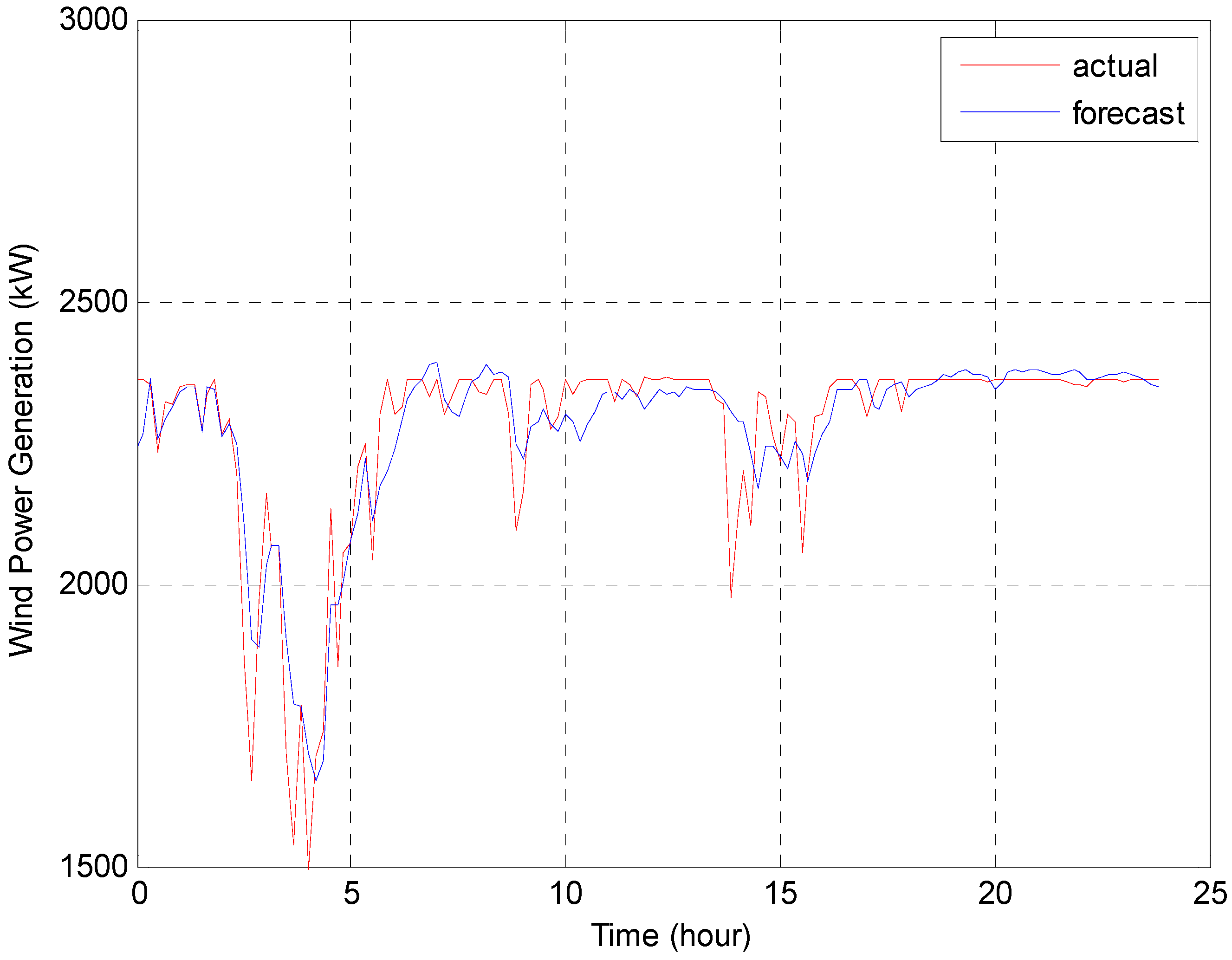
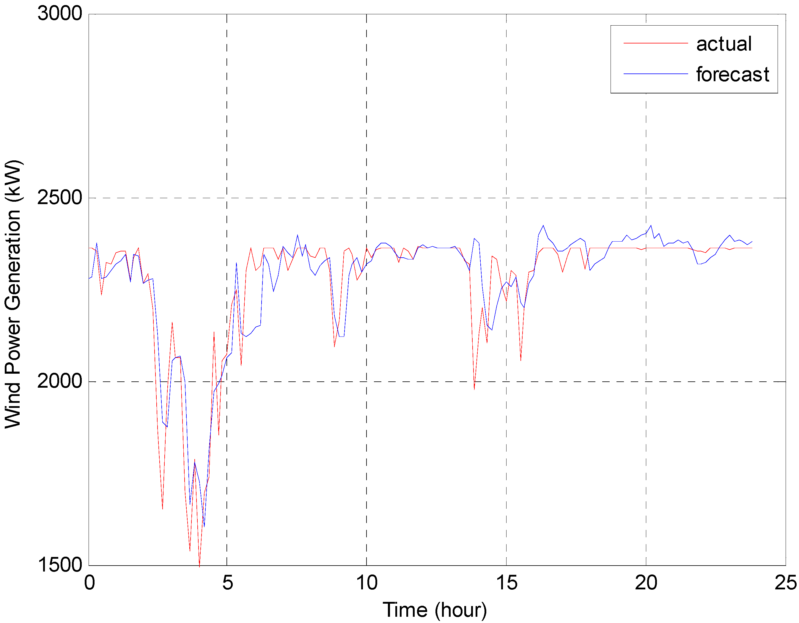
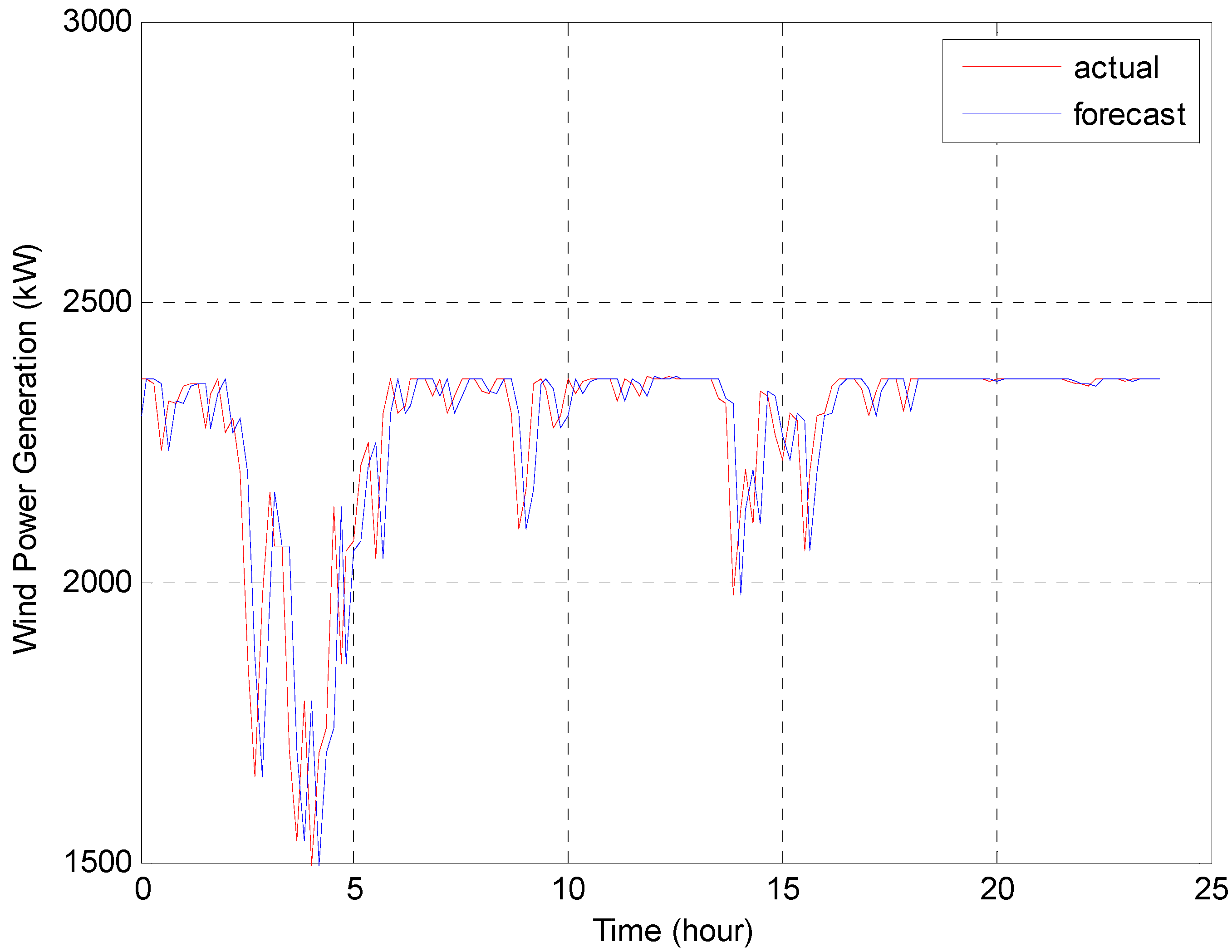
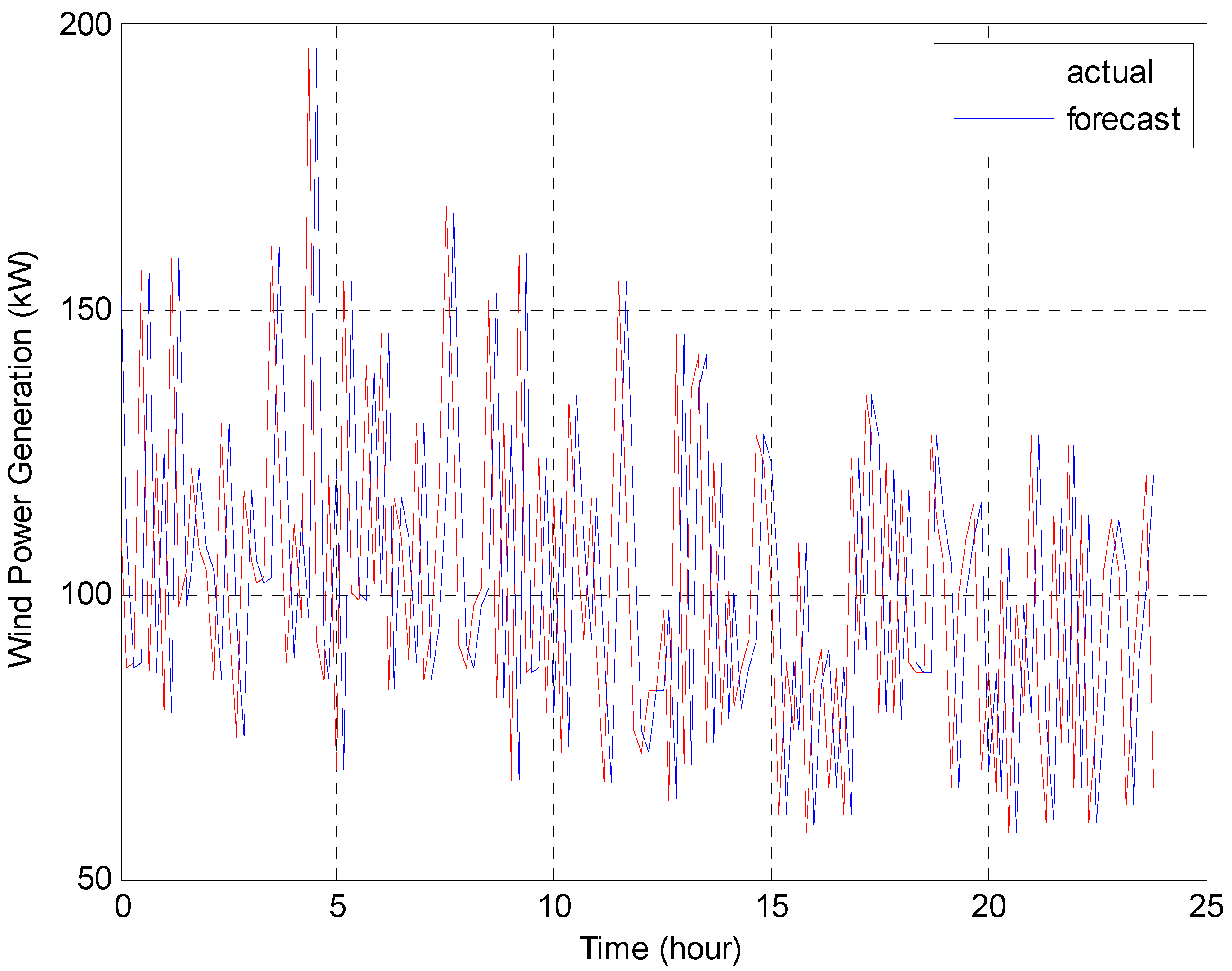
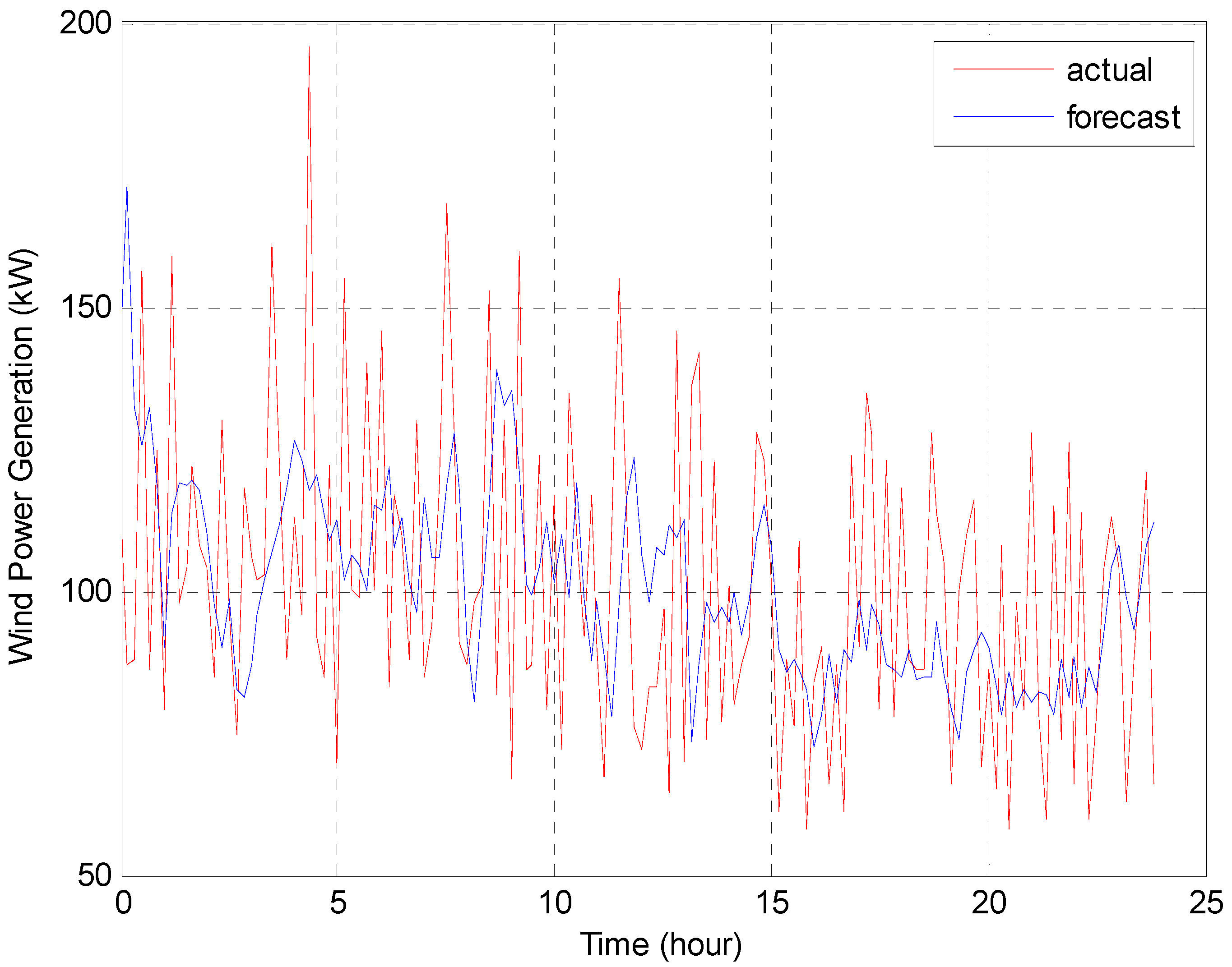
5. Numerical Results

To verify the proposed forecasting method, the method was used for wind power forecasting in Taiwan. Wind power forecasting was computed using the historical wind power and wind speed data every 10 min for a 2400 kW WECS installed in Taichung, on the coast of Taiwan. The wind power time series data for this WECS were recorded from 1 January 2008 to 31 December 2008, for one complete year. To ensure a clear comparison, no exogenous variables are considered. Because of seasonal atmospheric weather characteristics, the wind power and wind speed data are divided into four categories: spring, summer, autumn and winter. The proposed wind power forecast method is compared with the RBF neural network method, the persistence method, and the back propagation neural network method. The four season day test data results are shown below.

From the winter day data, the following days were selected: 1–5 December, 2008, corresponding to a typical winter day. The historical data set with 720 patterns were divided into a training data set for the RBF neural network and the back propagation neural network, of 576 patterns, collected from 1–4 December, and a test data set of 144 patterns, collected from 5 December.

The numerical results for the proposed hybrid method are shown in Figure 3.

Figure 3. Numerical results with the proposed hybrid method for typical winter day.

Figure 3. Numerical results with the proposed hybrid method for typical winter day.

The numerical results for the RBF neural network-based method are shown in Figure 4.

Figure 4. Numerical results with the RBF neural network based method for typical winter day.

Figure 4. Numerical results with the RBF neural network based method for typical winter day.

The numerical results for the persistence method are shown in Figure 5.

Figure 5. Numerical results with the persistence method for typical winter day.

Figure 5. Numerical results with the persistence method for typical winter day.

The numerical results for the back propagation neural network method are shown in Figure 6.

Figure 6. Numerical results with the back propagation neural network method for typical winter day.

Figure 6. Numerical results with the back propagation neural network method for typical winter day.

The forecasting error curves of the four methods for the winter days are shown in Figure 7.

Figure 7. The forecasting error curves of four methods for typical winter day.

Figure 7. The forecasting error curves of four methods for typical winter day.

From the summer day data, the following days were selected: 20–24 July 2008, corresponding to a typical summer day. The historical data set with 720 patterns were divided into a training data set for the RBF neural network and the back propagation neural network, of 576 patterns, collected from 20–23 July, and a test data set of 144 patterns, collected from 24 July. The numerical results for the proposed hybrid method are shown in Figure 8.

Figure 8. Test results with the proposed hybrid method for typical summer day.

Figure 8. Test results with the proposed hybrid method for typical summer day.

The numerical results for the RBF neural network-based method are shown in Figure 9.

Figure 9. Test results with the RBF neural network based method for typical summer day.

Figure 9. Test results with the RBF neural network based method for typical summer day.

The numerical results for the persistence method are shown in Figure 10.

Figure 10. Test results with the persistence method for typical summer day.

Figure 10. Test results with the persistence method for typical summer day.

The numerical results for the back propagation neural network method are shown in Figure 11.

Figure 11. Test results with the back propagation neural network method for typical summer day.

Figure 11. Test results with the back propagation neural network method for typical summer day.

The forecasting error curves of the four methods for the summer days are shown in Figure 12.

Figure 12. The forecasting error curves of four methods for typical summer day.

Figure 12. The forecasting error curves of four methods for typical summer day.

From the spring day data, the following days are selected: 1–5 March 2008, corresponding to a typical spring day. The training data set is collected from 1–4 March, and the test data set is collected from 5 March. From the autumn day data, the following days are selected: 20–24 October 2008, corresponding to a typical autumn day. The training data set is collected from 20–23 October, and the test data set is collected from 24 October.

Table 1 shows a comparison between the proposed EPSO-based hybrid method and three other methods (RBF neural network-based method, persistence method, back propagation neural network method). The performance of the proposed method is evaluated using two indices, namely the maximum absolute percentage error (MaxAPE) and the mean absolute percentage error (MAPE). The definitions of MaxAPE and MAPE are defined as follows:

$$MaxAPE=100\%\times Max(a_h-f_h)\hspace{1em}\hspace{1em}\begin{array}{cc}for& h=\begin{array}{ccc}1& to& N\end{array}\end{array}$$

(21)

$$MAPE=100\%\times \frac{1}{N}{\displaystyle \sum _{h=1}^N\frac{\left|a_h-f_h\right|}{a_h}}$$

(22)

where f_h and a_h are the forecasted and actual wind power at period h, respectively; N is the number of forecasted periods. In this paper, N equals to 144.

As shown in Table 1, the proposed EPSO-based hybrid method presents better forecasting accuracy for all four seasons. The MaxAPE has an average value of 61.59% with respect to the three previous methods are 65.16%, 109.40%, and 82.29%, respectively. The MAPE has an average value of 11.52% with respect to the three previous methods are 12.97%, 21.56%, and 17.61%, respectively.

Table 1. The accuracy evaluation of the four methods for wind power forecasting.

Season	Forecasting method	Maximum absolute percentage error	Mean absolute percentage error
Spring day	Proposed hybrid method	64.65%	6.57%
	RBF neural network-based method	68.42%	7.05%
	Persistence method	116.44%	8.49%
	Back propagation neural network method	69.91%	7.58%
Summer day	Proposed hybrid method	47.61%	12.38%
	RBF neural network-based method	53.67%	13.42%
	Persistence method	113.04%	35.42%
	Back propagation neural network method	102.25%	23.95%
Autumn day	Proposed hybrid method	117.44%	24.96%
	RBF neural network-based method	117.55%	28.98%
	Persistence method	186.67%	39.57%
	Back propagation neural network method	128.82%	34.37%
Winter day	Proposed hybrid method	16.65%	2.17%
	RBF neural network-based method	21.01%	2.41%
	Persistence method	21.44%	2.76%
	Back propagation neural network method	28.17%	4.53%

Table 1. The accuracy evaluation of the four methods for wind power forecasting.

Season	Forecasting method	Maximum absolute percentage error	Mean absolute percentage error
Spring day	Proposed hybrid method	64.65%	6.57%
	RBF neural network-based method	68.42%	7.05%
	Persistence method	116.44%	8.49%
	Back propagation neural network method	69.91%	7.58%
Summer day	Proposed hybrid method	47.61%	12.38%
	RBF neural network-based method	53.67%	13.42%
	Persistence method	113.04%	35.42%
	Back propagation neural network method	102.25%	23.95%
Autumn day	Proposed hybrid method	117.44%	24.96%
	RBF neural network-based method	117.55%	28.98%
	Persistence method	186.67%	39.57%
	Back propagation neural network method	128.82%	34.37%
Winter day	Proposed hybrid method	16.65%	2.17%
	RBF neural network-based method	21.01%	2.41%
	Persistence method	21.44%	2.76%
	Back propagation neural network method	28.17%	4.53%

Improvement in the average MaxAPE of the proposed EPSO-based hybrid method with respect to the three previous methods are 3.57%, 47.81%, and 20.7%, respectively. Improvement in the average MAPE of the proposed EPSO-based hybrid method with respect to the three previous methods are 1.45%, 10.04%, and 6.09%, respectively.

6. Conclusions

This paper proposes a hybrid method for 10 min ahead wind power forecasting. The proposed method uses the combination of a persistence method, a back propagation neural network and a RBF neural network. The application of the proposed method to short-term wind power forecasting is both novel and effective. The proposed wind power forecast method is compared with the RBF neural network method, persistence method and back propagation neural network method. An evaluation of the forecast methods is performed, using practical wind power generation information for a WECS. The results demonstrate the effectiveness of the proposed hybrid method and this method provided improved accuracy in the wind power forecasting.

References

1. Chang, W.Y. An RBF neural network combined with OLS algorithm and genetic algorithm for short-term wind power forecasting. J. Appl. Math. 2013, 2013. [Google Scholar] [CrossRef]
2. 2012 Half Year Report; The World Wind Energy Association: Bonn, Germany, 2012.
3. Wu, Z.; Zhu, C.; Hu, M. Improved control strategy for DFIG wind turbines for low voltage ride through. Energies 2013, 6, 1181–1197. [Google Scholar] [CrossRef]
4. Kabouris, J.; Kanellos, F.D. Impacts of large scale wind penetration on energy supply industry. Energies 2009, 2, 1031–1041. [Google Scholar] [CrossRef]
5. Sideratos, G.; Hatziargyriou, N.D. An advanced statistical method for wind power forecasting. IEEE Trans. Power Syst. 2007, 22, 258–265. [Google Scholar] [CrossRef]
6. Ma, L.; Luan, S.Y.; Jiang, C.W.; Liu, H.L.; Zhang, Y. A review on the forecasting of wind speed and generated power. Renew. Sustain. Energy Rev. 2009, 13, 915–920. [Google Scholar] [CrossRef]
7. Soman, S.S.; Zareipour, H.; Malik, O.; Mandal, P. A Review of Wind Power and Wind Speed Forecasting Methods with Different Time Horizons. In Proceedings of the 2010 North American Power Symposium (NAPS), Arlington, TX, USA, 26–28 September 2010; pp. 1–8.
8. Lange, M.; Focken, U. New Developments in Wind Energy Forecasting. In Proceedings of the 2008 IEEE Power and Energy Society General Meeting-Conversion and Delivery of Electrical Energy in the 21st Century, Pittsburgh, PA, USA, 20–24 July 2008; pp. 1–8.
9. Bhaskar, M.; Jain, A.; Srinath, N.V. Wind Speed Forecasting: Present Status. In Proceedings of the 2010 International Conference on Power System Technology (POWERCON), Hangzhou, China, 24–28 October 2010; pp. 1–6.
10. Bhaskar, K.; Singh, S.N. AWNN-assisted wind power forecasting using feed-forward neural network. IEEE Trans. Sustain. Energy 2012, 3, 306–315. [Google Scholar] [CrossRef]
11. Alexiadis, M.C.; Dokopoulos, P.S.; Sahsamanoglou, H.S. Wind speed and power forecasting based on spatial correlation models. IEEE Trans. Energy Convers. 1999, 14, 836–842. [Google Scholar] [CrossRef]
12. Alexiadis, M.C.; Dokopoulos, P.S.; Sahsamanoglou, H.S.; Manousaridis, I.M. Short-term forecasting of wind peed and related electrical power. Solar Energy 1999, 63, 61–68. [Google Scholar] [CrossRef]
13. Wu, Y.K.; Lee, C.Y.; Tsai, S.H.; Yu, S.N. Actual Experience on the Short-Term Wind Power Forecasting at Penghu-From an Island Perspective. In Proceedings of the 2010 International Conference on Power System Technology (POWERCON), Hangzhou, China, 24–28 October 2010; pp. 1–8.
14. Catalão, J.P.S.; Osório, G.J.; Pousinho, H.M.I. Short-Term Wind Power Forecasting Using a Hybrid Evolutionary Intelligent Approach. In Proceedings of the 16th International Conference on Intelligent System Application to Power Systems (ISAP), Hersonissos, Greece, 25–28 September 2011; pp. 1–5.
15. Zhao, X.; Wang, S.X.; Li, T. Review of evaluation criteria and main methods of wind power forecasting. Energy Procedia 2011, 12, 761–769. [Google Scholar] [CrossRef]
16. Chang, W.Y. Application of back propagation neural network for wind power generation forecasting. Int. J. Digit. Content Technol. Appl. 2013, 7, 502–509. [Google Scholar]
17. Wang, J.; Zhu, S.; Zhang, W.; Lu, H. Combined modeling for electric load forecasting with adaptive particle swarm optimization. Energy 2010, 35, 1671–1678. [Google Scholar] [CrossRef]
18. Kıran, M.S.; Özceylan, E.; Gündüz, M.; Paksoy, T. A novel hybrid approach based on particle swarm optimization and ant colony algorithm to forecast energy demand of Turkey. Energy Convers. Manag. 2012, 53, 75–83. [Google Scholar] [CrossRef]
19. Kennedy, J.; Eberhart, R.C. Particle Swarm Optimization. In Proceedings of the IEEE International Conference on Neural Networks, Perth, Australia, 27 November–01 December 1995; pp. 1942–1948.
20. Chaitou, H.; Nika, P. Exergetic optimization of a thermoacoustic engine using the particle swarm optimization method. Energy Convers. Manag. 2012, 55, 71–80. [Google Scholar] [CrossRef]
21. Bashir, Z.A.; El-Hawary, M.E. Applying wavelets to short-term load forecasting using PSO-based neural networks. IEEE Trans. Power Syst. 2009, 24, 20–27. [Google Scholar] [CrossRef]
22. Huang, C.M.; Wang, F.L. An RBF network with OLS and EPSO algorithms for real-time power dispatch. IEEE Trans. Power Syst. 2007, 22, 96–104. [Google Scholar] [CrossRef]